The effect of X-ray dust-scattering on a bright burst from the magnetar 1E 1547.0–5408

Abstract

A bright burst, followed by an X-ray tail lasting $\sim$10 ks, was detected during an XMM-Newton observation of the magnetar 1E 1547.0–5408 carried out on 2009 February 3. The burst, also observed by Swift/BAT, had a spectrum well fit by the sum of two blackbodies with temperatures of $\sim$4 keV and 10 keV and a fluence in the 0.3–150 keV energy range of $\sim 10^{-5}$ erg cm^-2. The X-ray tail had a fluence of $\sim 4\times 10^{-8}$ erg cm^-2. Thanks to the knowledge of the distances and relative optical depths of three dust clouds between us and 1E 1547.0–5408, we show that most of the X-rays in the tail can be explained by dust scattering of the burst emission, except for the first $\sim$20–30 s. We point out that other X-ray tails observed after strong magnetar bursts may contain a non-negligible contribution due to dust scattering.

1 Introduction

Dust grains in the interstellar medium cause small-angle scattering of soft X-ray photons. Due to this effect, if there is a significant amount of interstellar dust along the line of sight, bright point-like X-ray sources may appear surrounded by diffuse X-rays (the so-called “scattering halo”), as predicted by Overbeck (1965) and first observed by Rolf (1983) and Catura (1983). The study of such X-ray halos can provide important information on the properties of the interstellar dust (e.g. Mathis & Lee, 1991; Draine, 2003; Costantini et al., 2005).

Due to their longer path length, scattered X-rays have a time delay with respect to the unscattered ones. In the case of variable sources, this effect can be used to derive information on the source distance and the spatial distribution of the dust (Trümper & Schönfelder, 1973; Predehl et al., 2000; Miralda-Escudé, 1999). Short duration bursts scattered by thin layers of dust produce dust-scattering rings which appear to expand with time around the central source. Such rings were seen around galactic binary systems (e.g. Heinz et al., 2015; Heinz et al., 2016; Vasilopoulos & Petropoulou, 2016), magnetars (e.g. Tiengo et al., 2010; Svirski et al., 2011), and gamma-ray bursts (e.g. Vaughan et al., 2004; Tiengo & Mereghetti, 2006; Vianello et al., 2007).

The presence of delayed scattered radiation can also affect the time profile and spectrum of the X-rays detected after bright bursts. This must be taken into account when instruments with inadequate angular resolution, which do not permit to disentangle the scattered and unscattered components, are used. For example, it has been suggested that some of the X-ray afterglows of gamma-ray bursts, in particular those showing a long plateau phase, are due to scattering from dust in the host galaxies (Shao & Dai, 2007; Shao et al., 2008). Although Shen et al. (2009) showed that the lack of spectral evolution of most afterglows is inconsistent with this hypothesis, a few cases in which at least part of the X-ray emission can be explained by dust scattering have been recently reported (see, e.g., Holland et al., 2010; Evans et al., 2014; Wang et al., 2016).

In this work, we evaluate the effects of dust scattering on the observed properties of the X-ray tails seen after magnetar bursts, using, as a case study, an XMM-Newton observation of 1E 1547.0–5408 in which a burst followed by a decaying tail lasting $\sim$10 ks was detected. 1E 1547.0–5408 is a transient magnetar which showed three outburst episodes (Bernardini et al., 2011) and is surrounded by extended X-ray emission consistent with a dust scattering halo (Olausen et al., 2011). This source is particularly suitable for our investigation since, thanks to previous analysis of three dust scattering rings caused by a much brighter burst, some of the properties of the dust in this direction are already known (Tiengo et al., 2010).

In Section 2 we present the data reduction of the XMM-Newton  and Swift observations; in Section 3 we first characterize the properties of the persistent emission and of the burst of 1E 1547.0–5408 and then analyze the time evolution of the radial profiles of the X-ray tail and we fit the tail light curve and spectrum with a dust scattering model. We discuss our results in Section 4, where we also compare this event from 1E 1547.0–5408 with other magnetar bursts and flares followed by extended tails.

2 data reduction

We analyzed an XMM-Newton observation of 1E 1547.0–5408, with exposure time of $\sim$56 ks, taken on 2009 February 3. This is the same observation used by Tiengo et al. (2010) to study the dust scattering rings produced by a bright burst that occurred on January 22 (Mereghetti et al., 2009). We note that the presence of such rings, at angular distance larger than 3^′ from the central source, does not affect the analysis presented here.

The three cameras of the EPIC instrument, one pn camera (Strüder et al., 2001) and two MOS cameras (Turner et al., 2001), were operated in full-frame mode and with a thick optical blocking filter. We reduced the data with the SAS v.14.0.0 software, selecting single- and double-pixel events (pattern$\leq$4) for the pn and single- and multiple-pixel events for the MOS (pattern$\leq$12). Because of its high count rate ($>6$ cts s^-1 in the EPIC-pn), the source data were affected by pile-up, therefore we extracted the source spectra and lightcurves from an annular region with inner and outer radii of 5^′′ and 40^′′, respectively. The background was extracted from a circular region of radius 60^′′ free of sources. For the RGS instrument we obtained the source events following the standard procedures described in the SAS threads.

We also used a Swift/BAT observation (Obs.ID: 00341965000) taken almost simultaneously with the XMM-Newton one. Spectra and lightcurves were extracted following the standard data reduction procedures described in the Swift/BAT threads.

The spectral fits were carried out with the xspec v.12.8.2 software package, adopting the phabs model, with the solar abundances of Wilms et al. (2000), for the interstellar absorption. All the errors in the spectral parameters reported below are at the 90% confidence level for a single interesting parameter.

3 Data analysis and results

Figure 1: EPIC-pn lightcurve of 1E 1547.0–5408  in the energy range 0.3–10 keV binned at 1 s. Several bursts are clearly visible. The strongest (and saturated) burst at T=0 is the one with the X-ray tail considered in this work.

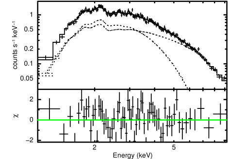
Figure 2: Top panel: EPIC-pn spectrum of the persistent emission of 1E 1547.0–5408 derived from the last $\sim$9 ks of the XMM-Newton observation. The solid line represents the best-fiting model, which consists of a powerlaw (dashed) plus a blackbody (point-dashed). Bottom panel: residuals of the best-fitting (rebinned for display purposes).

During the XMM-Newton observation, 1E 1547.0–5408 emitted several short bursts (Fig. 1). In this work we concentrate on the brightest one, which was followed by a tail of enhanced X-ray emission lasting about 10 ks. In the analysis of the EPIC data, we removed short time intervals corresponding to all the fainter bursts visible during the observation.

We derived the properties of the persistent emission of 1E 1547.0–5408  from the last $\sim$9 ks of the XMM-Newton observation, when the source had the lowest count rate and no bursts were emitted. We extracted the EPIC-pn spectrum, in the energy range 1–10 keV, from this time interval and fitted it with the phenomenological model usually adopted for magnetars in this energy range, i.e. an absorbed blackbody plus power-law model (Mereghetti, 2008). We obtained a good fit ($\chi^{2}/dof=139.55/128$, see Fig. 2) with the following parameters: column density N_H=$(4.2\pm 0.3)\times 10^{22}$ cm^-2, blackbody temperature kT=0.64$\pm$0.03 keV, emitting radius $R$=$(1.8\pm 0.2)\cdot d_{4\text{kpc}}$ km, power-law photon index $\Gamma$=1.8$\pm$0.3 and normalization F_1keV=$1_{-0.5}^{+0.8}\times 10^{-2}$ photons cm^-2 s^-1 keV^-1. The absorbed and unabsorbed fluxes in the 1–10 keV energy range are $(4.59\pm 0.06)\times 10^{-11}$ erg cm^-2 s^-1 and $(8.3\pm 0.2)\times 10^{-11}$ erg cm^-2 s^-1, respectively. These results are consistent with those reported by Bernardini et al. (2011), who did not exclude the time interval of the burst tail from their spectral analysis.

Figure 3: Swift/BAT lightcurve of the bright burst in the 15-150 keV energy range with a bin size of 1 ms.

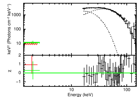
Figure 4: Swift/BAT (black) and RGS (green and red) fluence spectra of the burst. Top panel: best fit with the sum of two blackbody models. Bottom panel: residuals of the best fit.

3.1 Burst properties

The initial part of the brightest burst could not be studied with EPIC because the saturation effect due to the high count rate caused a severe loss of photons. Therefore, to derive the burst fluence, we used the Swift/BAT and the RGS data which were not affected by saturation.

The BAT data show that the burst started at T₀=20:00:39.47 UT of 2009 February 3. Its light curve, in the energy range 15–150 keV (Fig. 3), was characterized by a bright peak lasting $\sim$0.1 s, followed by fainter emission lasting about 0.2 s. The burst was also clearly visible in the RGS data, with a start time consistent with the above value, considering the limited time resolution of the two cameras (read-out times of $\sim$5 s and $\sim$10 s).

To estimate the burst fluence, we extracted the BAT and RGS1 and RGS2 spectra of the burst events only, for time intervals of $\sim 30$ ms and 10 s, respectively. Since at these time scales the persistent emission contribution is negligible, we studied the burst spectrum in fluence units by assigning an exposure time of 1 s to both RGS and BAT spectra. Despite the low RGS count statistics allowed us to use only a single energy bin for each camera (0.3–2 keV), these measurements, when fitted together with the BAT spectrum, could constrain the burst spectral shape at low energies. We fitted the spectra simultaneously in the range 0.3–150 keV, with the column density fixed at the value of $4.2\times 10^{22}$ cm^-2 derived for the persistent emission. The best-fit was obtained with the sum of two blackbody models, as found for the spectra of the short bursts of other magnetars in similar energy ranges (Feroci et al., 2004; Israel et al., 2008). Our best fit gave temperatures kT₁ = $4.1\pm 0.4$ keV and kT₂ = $9.8\pm 0.4$ keV and emitting radii R${}_{1}=(14.8\pm 3.0)\,d_{4\text{kpc}}$ km and R${}_{2}=(3.1\pm 0.3)\,d_{4\text{kpc}}$ km ($\chi^{2}/dof=44.74/56$; Fig. 4). The absorbed (unabsorbed) fluence in the range 0.3–150 keV was $9.7\times 10^{-6}$ erg cm^-2 ($9.9\times 10^{-6}$ erg cm^-2), while in the 4–10 keV range it was $1.1\times 10^{-6}$ erg cm^-2 ($1.2\times 10^{-6}$ erg cm^-2).

3.2 Timing and spatial analysis of the burst tail

The bright burst described in the previous subsection was followed by an extended tail of X-ray emission (Fig. 5). The initial part of the tail showed a steep power law decay with $F(t-T_{0})\propto(t-T_{0})^{-(2.3\pm 0.9)}$ cts s^-1, while the following part, with the exception of a rebrightening at $t-T_{0}\sim 200$ s, can be described by an exponential function, $F(t-T_{0})=(0.47\pm 0.09)e^{-(t-T_{0})/(2496\pm 473)}$ cts s^-1.

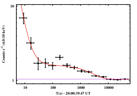
Figure 5: 4–10 keV EPIC-pn lightcurve of the tail after the main burst. The horizontal line indicates the level of the persistent emission. The red line is the fit with a power-law and an exponential as described in the text.

To study the angular distribution of the tail emission and its time evolution, starting from the burst epoch, we built the radial profiles for several, consecutive, time intervals of different durations from the summed pn and MOS images. We subtracted from these profiles the radial profile of the persistent emission, derived from the same time interval used for the spectral analysis. The resulting net radial profiles, shown in Fig. 6, suggest the presence of excess emission at an angular distance which increases with time. The fit of the radial profiles with a King function (as expected for the EPIC PSF) was not acceptable ($\chi^{2}_{\nu}>2$) in all but the first two time intervals, clearly indicating time variability of the profiles, possiby due to the presence of dust-scattering expanding rings. Note that these deviations from a King profile cannot be attributed to pile-up, since the importance of this effect increases with the source count-rate and it should therefore affect the first time intervals rather than the ones found to be inconsistent with the PSF. We fitted the net radial profiles with a Lorentzian (see Tiengo et al. 2010), plus a constant to account for variable diffuse emission on large spatial scales. We fixed the width of the Lorentzian to 10^′′, corresponding to the value expected for a geometrically-thin ring profile broadened by the EPIC PSF. With this model we found a significant improvement in the quality of the fits for all the radial profiles ($\chi^{2}_{\nu}\sim 1$; Fig. 6).

The evolution of the centroid of the Lorentzian component as a function of time is shown in the left panel of Fig. 7. We fitted the centroid values with the model expected to describe the angular expansion, $\theta(t)=K(t-T_{0})^{0.5}$, and we found $K=0.884\pm 0.045$ arcmin day^-0.5 (error at $1\sigma$). This value is fully consistent with the value K=0.8845$\pm$0.0008 reported in Tiengo et al. (2010) for the farthest of the three dust layers present between us and 1E 1547.0–5408. We could better estimate $K$ by fitting the new data points together with those reported in Tiengo et al. (2010) (right panel of Fig. 7). The best fit gave $\chi^{2}/dof=25.31/15$ and $K=0.8847\pm 0.0008$ arcmin day^-0.5. If instead we fit the new points with those associated to the other two dust layers, we obtain significantly poorer fits (reduced $\chi^{2}>2$). Finally, we also searched for the rings produced by the other two dust layers in the radial profiles by fitting them with two additional Lorentzian components, but they were too weak to be detected.

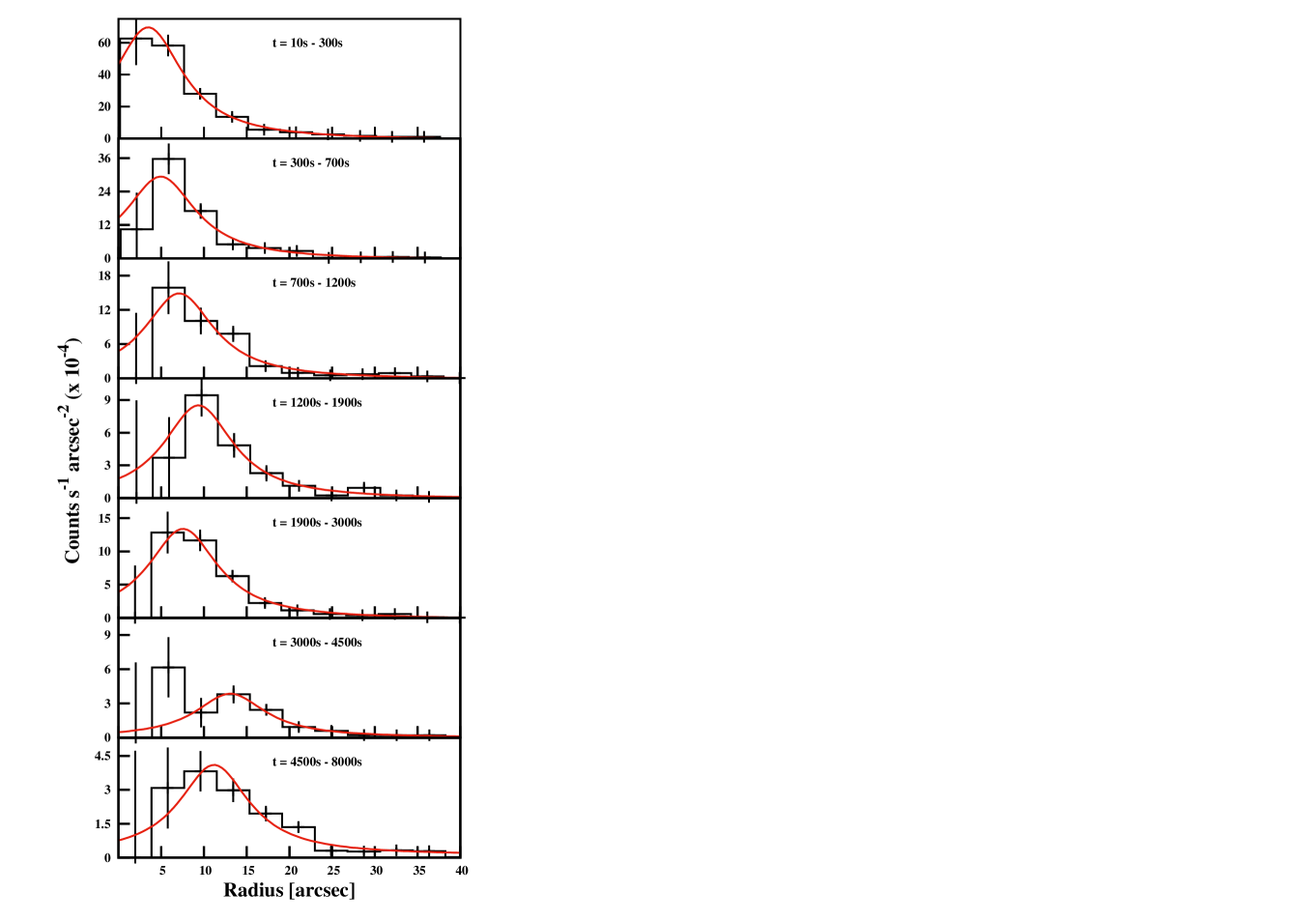
Figure 6: Radial profiles of summed EPIC-pn and MOS data at different time intervals starting from the burst, after subtracting the profile of the persistent emission. The solid line is the best fit of the profile using a constant plus a lorentzian function. The data clearly show a ring expanding and fading with time.

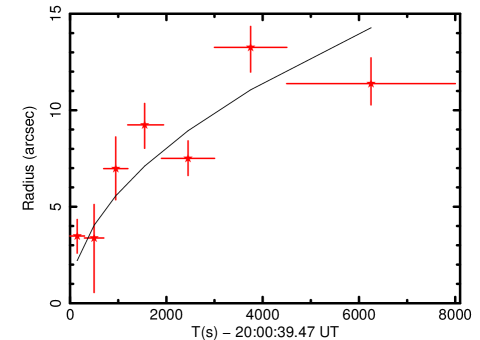
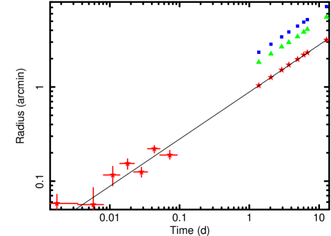
Figure 7: Left: angular size of the inner ring as a function of time; each point (red) was obtained by fitting with a constant plus a lorentzian model the radial profile obtained in consecutive bin times (with varying length) starting from the burst; the solid line is the best fit $\theta(t)=(0.884\pm 0.045)\cdot t^{0.5}$. Right: joint fit with the points taken from Tiengo et al. (2010). The red stars, green triangles, and blue squares indicate the angular radii of the three rings caused by the burst of January 22. Error bars are at 1$\sigma$ in both figures.

3.3 Dust scattering modelling of the tail light curve

The above results indicate that at least part of the tail emission is consistent with a dust scattering ring which was expanding at the same rate measured by Tiengo et al. (2010) for the inner ring produced by the strong burst of January 22.

As a further check, we computed the light curve expected for the scattered emission in the 4–10 keV band, where the tail is more evident. We adopted the grain model that gave the best fit to the data of Tiengo et al. (2010), i.e. the BARE-GR-B model of Zubko et al. (2004), and the corresponding distances for 1E 1547.0–5408 (3.9 kpc) and for the three dust layers (3.4, 2.6 and 2.2 kpc).

We used the spectral distribution and fluence of the burst derived in section 3.1 and included the effect of the three dust layers with column densities fixed at $1\times 10^{22}$, $0.24\times 10^{22}$ and $0.27\times 10^{22}$ cm^-2 (Tiengo et al., 2010). We also assumed that the dust layers are geometrically thin and that the burst was instantaneous.

In Fig. 8 we compare the computed lightcurve (red line) with the observed data. Clearly, we cannot reproduce the data with the above column density values. Instead, we found that a $\sim$3.5 times higher column density in the three dust layers is required to describe the tail lightcurve after the first $\sim 20$ s (blue line in Fig. 8).

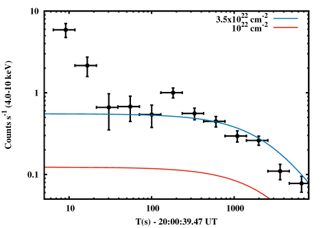
Figure 8: Comparison between the 4–10 keV EPIC-pn lightcurve (black points, persistent emission subtracted), and the simulated lightcurves of dust-scattering for the BARE-GR-B grains model (Zubko et al., 2004). The column density of the farthest dust layer is $10^{22}$ cm^-2 (red line) and $3.5\times 10^{22}$ cm^-2 (blue line).

3.4 Spectral analysis of the tail

The results described above indicate that the angular distribution and the light curve of the X-ray tail, at least for times greater than $\sim T_{0}$+20 s, are consistent with those expected for dust scattering. Here we investigate whether also the spectral properties of the tail emission are consistent with this hypothesis.

We created an xspec table model with the spectra expected for the scattered emission. We computed it for a range of distances of 1E 1547.0–5408  (from 0.1 to 10 kpc) and using again the BARE-GR-B dust model. For each value of the source distance, the relative distances of the three dust layers are determined by the measured rates of expansion of the rings (Tiengo et al., 2010). We assumed that the optical depths of the two closer dust layers are 24% and 27% of that of the layer responsible for the inner ring. We fixed the burst spectrum and its fluence as done above for the light curve computation. Therefore, the table model has only two parameters: source distance and column density of the farthest dust layer, N${}_{\text{H1}}$.

We fitted the pn spectrum of the tail extracted in the time interval from $T_{0}+20$ s to $T_{0}+4$ ks. The limit of 4 ks was chosen because, for longer exposure times, the signal-to-noise ratio of the spectrum is too low. The contribution of the persistent emission was included in the fit, with parameters fixed at the best-fit blackbody plus powerlaw model described above.

Since the source distance was poorly constrained, we fixed it at 3.9 kpc and found a very good fit ($\chi^{2}$/dof = 62.79/67) with N${}_{\text{H1}}=(4.0\pm 0.4)\times 10^{22}$ cm^-2 (see Table 1 and Fig. 9). The total column density in the three dust layers, N${}_{\text{H1}}\times(1+0.24+0.27)=(6.0\pm 0.6)\times 10^{22}$ cm^-2 is about a 40% larger than that derived from the fit of the persistent emission (N${}_{\text{H1}}=4.2\times 10^{22}$ cm^-2). Fixing N${}_{\text{H1}}=2.78\times 10^{22}$ cm^-2, to avoid exceeding the total absorption of the persistent emission, requires an additional blackbody to fit the spectrum. Its parameters are kT $=1.2$ keV and emitting radius of R $=167_{-167}^{+95}$ m. Such a thermal component can be attributed to the emission from a small region on the NS surface that has been heated by the energy released in the burst. Although the current data yield relatively large errors on the best fit parameters, we note that by completely neglecting the dust scattering, one would obtain different results. In fact, if we assume that there is no dust scattering contribution in the tail, it is still possible to obtain a good fit ($\chi^{2}/dof=49.97/66$) by adding to the persistent emission a blackbody with a slightly higher temperature kT =$1.8_{-0.2}^{+0.3}$ keV, emitting radius R $=135_{-30}^{+35}$ m, and flux of $(7.1\pm 1.0)\times 10^{-12}$ erg cm^-2 s^-1 (4–10 keV unabsorbed, see Table 1).

Table 1: Spectral results for the burst tail

	blackbody		dust scattering
	kT	Radiusa	N${}_{\text{H1}}^{b}$	Fluxc	$\chi^{2}$/dof
	(keV)	(m)	($10^{22}$ cm-2)	( 10-12 erg cm2 s-1)
Only NS	$1.8^{+0.3}_{-0.2}$	$135^{+35}_{-30}$	-	-	49.97/66
Only dust	-	-	4.0$\pm$0.4	9.9$\pm$1.1	62.79/67
NS+dust	$1.2^{+0.4}_{-0.2}$	$167^{+35}_{-167}$	2.78 (fixed)	5.7$\pm$0.7	50.90/66

Notes: The model of the persistent emission has been included in all the fits with fixed parameters (see text). The total absorption and the source distance have been fixed at N${}_{\text{H}}=4.2\times 10^{22}$ cm^-2 and d=3.9 kpc, respectively. Errors at $90\%$ confidence level.

^a Blackbody emitting radius for d=3.9 kpc.

^b Column density of farthest dust layer.

^c Average flux in the 0.3–10 keV range (unabsorbed).

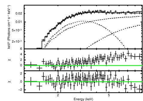
Figure 9: Top panel: spectrum of the tail integrated for 4 ks after the burst. The solid line is the best-fit model, while the dashed lines represent the blackbody, powerlaw, and dust-scattering components. Center panel: residuals of the fit when adopting only the best fit model of the persistent emission. Bottom panel: residuals of the fit when adding the dust-scattering component to the persistent emission.

4 Discussion

In this work we studied a long-lasting X-ray tail emitted from the magnetar 1E 1547.0–5408 after a bright short burst on 2009 February 3. The burst consisted of a bright peak lasting about 0.1 s, with fluence, derived with a joint spectral analysis of Swift/BAT and XMM-Newton/RGS data, of $\sim 10^{-5}$ erg cm^-2 (0.3-150 keV). The X-ray tail was characterized by a steep initial decay, with a duration of about 20 s, followed by a slower decrease, lasting at least 8 ks and with a fluence of $\sim 4\times 10^{-8}$ erg cm^-2. We found evidence for an angular expansion of the X-ray emission during the tail and, thanks to the previous knowledge of the properties of the dust clouds in the direction of 1E 1547.0–5408  (Tiengo et al., 2010), we showed that the part of the tail starting $\sim$20–30 s after the burst can be entirely explained by dust-scattering.

Table 2: Bursts and flares with extended X-ray tails in magnetars.

Source	Burst	F${}_{BURST}^{a}$	Tail duration	F${}_{TAIL}^{a}$	Ref.b	Notes
(distance)	date	(erg cm-2)	(ks)	(erg cm-2)
SGR 1900+14	1998/08/27	$>$8$\cdot 10^{-3}$	0.4	1.3$\cdot 10^{-2}$	M99	Giant flare
(14 kpc)	1998/08/29	1.4$\cdot 10^{-4}$	$\sim$8	6.7$\cdot 10^{-7}$	I01,L03
	2001/04/28	1.8$\cdot 10^{-4}$	$\sim$4	2.8$\cdot 10^{-7}$	L03
SGR 1806–20	2004/06/22	1.8$\cdot 10^{-5}$	$\sim$0.9	3$\cdot 10^{-8}$	G11
(8.7 kpc)	2004/10/17	1.3$\cdot 10^{-4}$	$>$1.3	7$\cdot 10^{-7}$	G11
	2004/12/27	1.4	0.4	2.5$\cdot 10^{-2}$	F07	Giant flare
SGR 0526–66	1979/03/05	5$\cdot 10^{-4}$	0.2	4$\cdot 10^{-3}$	M99	Giant flare
(55 kpc)
1E 1547–5408	2009/01/22	$>$6$\cdot 10^{-5}$	0.00785	6.9$\cdot 10^{-4}$	M09,T10	Tail at E$>$80 keV
(3.9 kpc)	2009/01/22	2.65$\cdot 10^{-7}$	0.017	5.97$\cdot 10^{-8}$	M15
	2009/02/03	9.9$\cdot 10^{-6}$	$\sim$8	3.7$\cdot 10^{-8}$	This work	Total tail emission
			$\sim$0.030	1.8$\cdot 10^{-9}$	This work	Corrected for dust scattering
	2009/02/06	1.29$\cdot 10^{-9}$	3.534	2.9$\cdot 10^{-7}$	M15
	2009/03/30	4.3$\cdot 10^{-7}$	0.624	3.1$\cdot 10^{-8}$	M15,K12
	2010/01/11	1.1$\cdot 10^{-8}$	0.773	4.9$\cdot 10^{-8}$	M15,K12
4U 0142+61	2006/06/25	2$\cdot 10^{-9}$	$>$0.463	2.86$\cdot 10^{-8}$	C16
(3.5 kpc)	2007/02/07	4.17$\cdot 10^{-8}$	$>1.6$	1.58$\cdot 10^{-7}$	C16
	2015/02/28	7.63$\cdot 10^{-8}$	0.3	$>$9.5$\cdot 10^{-8}$	G16
XTE J1810–197	2004/02/16	$>$6.5$\cdot 10^{-9}$	$>0.575$	$>$3.9$\cdot 10^{-8}$	W05
(5 kpc)

^a Unabsorbed fluence in the range 0.3–150 keV.

^b C16: Chakraborty et al. (2016); F07: Frederiks et al. (2007); G11: Göǧüş et al. (2011); G16: Gogus et al. (2016); I01: Ibrahim et al. (2001); K12: Kuiper et al. (2012); L03: Lenters et al. (2003); M09: Mereghetti et al. (2009); M99: Mazets et al. (1999); M15: Muş et al. (2015); T10: Tiengo et al. (2010); W05: Woods et al. (2005);

The total column density derived from our fit of the X-ray tail with a dust scattering model ($N_{\rm H}=6\times 10^{22}$ cm^-2) is slightly larger than that obtained in the spectral analysis of the persistent emission of 1E 1547.0–5408  ($N_{\rm H}=4.2\times 10^{22}$ cm^-2). Such an apparent discrepancy is likely related to the fact that the gas-to-dust ratio is not uniform in the Galaxy, while the normalization of the adopted dust model (number of grains per H atom) is based on an average value. In particular, the comparison between the $N_{\rm H}$ derived from X-ray spectra and the reddening in stars behind nearby molecular clouds indicates, as in our results, an excess of dust with respect to gas in dense clouds (see, e.g., Vuong et al., 2003; Hasenberger et al., 2016). On the other hand, if also unscattered emission from 1E 1547.0–5408 contributes to the tail, a lower column density of dust is required (see Table 1). Note, however, that such a contribution must be small because, although the tail spectrum is compatible with thermal emission from a fraction of the NS surface, the spatial analysis described in Sect. 3.2 shows that most of the tail emission is produced by dust scattering.

The steep part of the X-ray tail at $t<T_{0}+$20 s cannot be reproduced by the dust scattering model used to describe it at later times. In principle, it could be explained by invoking the presence of a dense dust layer very close (less than a few pc) to the source, possibly related to the supernova remnant associated with 1E 1547.0–5408 (Gelfand & Gaensler, 2007). However, it is more likely that the first part of the X-ray tail is dominated by unscattered emission, which comes directly from 1E 1547.0–5408. This emission could originate, for example, in a region of the NS surface which has been heated by the burst or in a trapped fireball in the star magnetosphere (Thompson & Duncan, 1995). Unfortunately, the small number of counts did not allow us to confirm this with a significant detection of pulsations in the first 20–30 s.

To put our results in the context of other similar events, we compiled in Table 2 the properties of several bursts followed by X-ray tails detected in 1E 1547.0–5408 and in other magnetars. We included, for comparison, also the three giant flares from SGR 0526–66, SGR 1806–20, and SGR 1900$+$14, although they involved a much larger energy budget (see Mereghetti, 2008, and references therein). Based on the best available spectral and timing information reported in the literature, we estimated for each event the fluence of the tail and that of the associated initial burst and, using the distances given in Table 2, we derived the energies plotted in Fig. 10. Note that some of these estimates have relatively large uncertainties due to the poorly constrained spectra and/or instrumental saturation effects (in some cases, only lower limits could be established).

For the burst of 1E 1547.0–5408 we plotted two values in Fig. 10: one in which we consider the whole energy of the tail and one in which we exclude the part attributed to dust scattering. For the latter we only considered the fluence of the first part of the tail, estimated by its EPIC-pn spectrum. The fluence of the short burst corresponds to a total energy release of $\sim 2\times 10^{40}\,d^{2}_{4\text{kpc}}$ erg. Therefore, this was a relatively strong burst, although not as energetic as the brighter events seen from this source on 2009 January 22 (Mereghetti et al., 2009; Savchenko et al., 2010).

From Fig. 10, it is clear that magnetar bursts span a large range of intensities, with several events with “intermediate” energy outputs, which bridge the “standard” bursts with the much rarer giant flares. Although there is an overall correlation between the burst and tail energetics, especially when also the giant and intermediate flares are considered, the data show a large dispersion. The energy in the tail can be either a fraction of that of the burst or exceed it. The latter case seems to require an additional energy supply released on a longer timescale after the burst, but the analysis of 1E 1547.0–5408  reported here shows that, in some cases, the tail energy might be overestimated if assuming an intrinsic NS emission only.

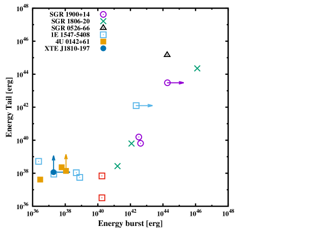
Figure 10: Energy of the tails versus the energy of their corresponding bursts (see Table 2). The red squares refer to the burst of 2009 February 3, uncorrected and corrected for the dust scattering contribution to the observed tail fluence.

4.1 Implications for the burst of 2009 January 22

Tiengo et al. (2010) studied three bright dust scattering rings around 1E 1547.0–5408. Their angular expansion rate measured with XMM-Newton and Swift, clearly indicates that they were produced by one (or possibly more) of the very luminous bursts seen by INTEGRAL in the time interval from 6:43 to 6:51 UT of 2009 January 22 (Mereghetti et al., 2009). Unfortunately, the fluence of these bursts in the soft X-ray band (0.5-10 keV) was not measured directly, since they were observed only in the hard X-ray range and, furthermore, the two brightest ones saturated the instruments. For this reason, Tiengo et al. (2010) could obtain only a combined information of the two factors which determine the flux of the scattered radiation, i.e. the dust optical depth and the fluence of the burst.

This degeneracy can now be removed because, for the burst of February 3 analyzed in this work, both the unscattered and scattered X-ray fluences have been measured: if the tail after T₀+20 s is entirely due to dust scattering, a column density $N_{\rm H1}=4\times 10^{22}$ cm^-2 is required for the farthest of the three dust clouds. This is four times larger than the value assumed by Tiengo et al. (2010) and implies that the January 22 burst emitted $2.5\times 10^{43}\,d^{2}_{4\text{kpc}}$ erg ($4.75\times 10^{43}\,d^{2}_{4\text{kpc}}$ erg) in the 1-100 keV range, for a thermal bremsstrahlung spectrum with temperature kT = 30 keV (100 keV). These values are a factor of 4 smaller than those reported in Tiengo et al. (2010).

5 Conclusions

We have shown that most of the long lasting X-ray emission detected after a burst of the magnetar 1E 1547.0–5408 can be explained as radiation scattered by interstellar dust. In fact, based on previous observations of expanding rings after a brighter event, there is solid evidence for the presence of a significant amount of dust concentrated in three clouds along the line of sight of this source. The effect of this dust on fainter bursts, such as the one analyzed here, is certainly less spectacular, but it cannot be neglected. Indeed, by ignoring it, one would attribute the whole X-ray tail, lasting about 10 ks and with a fluence of $\sim 4\times 10^{-8}$ erg cm^-2, to enhanced emission coming directly from 1E 1547.0–5408 and related to the burst.

Can a similar scenario apply also to other X-ray tails observed after the bursts of different magnetars? Most of these sources are located in the Galactic plane, at distances of several kiloparsecs, and have absoption values similar to, and in a few cases larger than, that of 1E 1547.0–5408. Undoubtedly, their radiation is subject to some scattering, as demonstrated by the long-lived halos observed around SGR 1806–20 (Kaplan et al., 2002), SGR 1900+14 (Kouveliotou et al., 2001), SGR 1833–0832 (Esposito et al., 2011), Swift J1834.9–0846 (Esposito et al., 2013), and SGR J1935+2154 (Israel et al., 2016). On the other hand, some X-ray emission after bright bursts must come directly from the neutron star. This is evident when pulsations are observed, while the interpretation of unpulsed emission, often showing a hard to soft spectral evolution which suggests a cooling region on the NS, is subject to more uncertainties. Often the quality of the data is insufficient to disentangle the contribution of dust scattering from that of the intrinsic emission in the observed X-ray tails. Unfortunately, a quantitative assessment of this effect, as we did for 1E 1547.0–5408, can be done only when bright bursts are observed and timely follow-ups with good imaging and sensitivity are carried out to study the X-ray halo evolution.

References

- Bernardini et al. (2011) Bernardini F., Israel G. L., Stella L., Turolla R., Esposito P., Rea N., Zane S., Tiengo A., Campana S., Götz D., Mereghetti S., Romano P., 2011, A&A, 529, A19
- Bernardini et al. (2011) Bernardini F., Perna R., Gotthelf E. V., Israel G. L., Rea N., Stella L., 2011, MNRAS, 418, 638
- Catura (1983) Catura R. C., 1983, ApJ, 275, 645
- Chakraborty et al. (2016) Chakraborty M., Göğüş E., Şaşmaz Muş S., Kaneko Y., 2016, ApJ, 819, 153
- Costantini et al. (2005) Costantini E., Freyberg M. J., Predehl P., 2005, A&A, 444, 187
- Draine (2003) Draine B. T., 2003, ApJ, 598, 1026
- Esposito et al. (2011) Esposito P., et al., 2011, MNRAS, 416, 205
- Esposito et al. (2013) Esposito P., Tiengo A., Rea N., Turolla R., Fenzi A., Giuliani A., Israel G. L., Zane S., Mereghetti S., Possenti A., Burgay M., Stella L., Götz D., Perna R., Mignani R. P., Romano P., 2013, MNRAS, 429, 3123
- Evans et al. (2014) Evans P. A., et al., 2014, MNRAS, 444, 250
- Feroci et al. (2004) Feroci M., Caliandro G. A., Massaro E., Mereghetti S., Woods P. M., 2004, ApJ, 612, 408
- Frederiks et al. (2007) Frederiks D. D., Golenetskii S. V., Palshin V. D., Aptekar R. L., Ilyinskii V. N., Oleinik F. P., Mazets E. P., Cline T. L., 2007, Astronomy Letters, 33, 1
- Gelfand & Gaensler (2007) Gelfand J. D., Gaensler B. M., 2007, ApJ, 667, 1111
- Gogus et al. (2016) Gogus E., Lin L., Roberts O. J., Chakraborty M., Kaneko Y., Gill R., Granot J., van der Horst A. J., Watts A. L., Baring M., Kouveliotou C., Huppenkothen D., Younes G., 2016, ArXiv e-prints
- Göǧüş et al. (2011) Göǧüş E., Woods P. M., Kouveliotou C., Finger M. H., Pal’shin V., Kaneko Y., Golenetskii S., Frederiks D., Airhart C., 2011, ApJ, 740, 55
- Hasenberger et al. (2016) Hasenberger B., Forbrich J., Alves J., Wolk S. J., Meingast S., Getman K. V., Pillitteri I., 2016, A&A, 593, A7
- Heinz et al. (2015) Heinz S., Burton M., Braiding C., Brandt W. N., Jonker P. G., Sell P., Fender R. P., Nowak M. A., Schulz N. S., 2015, ApJ, 806, 265
- Heinz et al. (2016) Heinz S., Corrales L., Smith R., Brandt W. N., Jonker P. G., Plotkin R. M., Neilsen J., 2016, ApJ, 825, 15
- Holland et al. (2010) Holland S. T., Sbarufatti B., Shen R., Schady P., Cummings J. R., Fonseca E., Fynbo J. P. U., Jakobsson P., Leitet E., Linné S., Roming P. W. A., Still M., Zhang B., 2010, ApJ, 717, 223
- Ibrahim et al. (2001) Ibrahim A. I., Strohmayer T. E., Woods P. M., Kouveliotou C., Thompson C., Duncan R. C., Dieters S., Swank J. H., van Paradijs J., Finger M., 2001, ApJ, 558, 237
- Israel et al. (2016) Israel G. L., Esposito P., Rea N., Coti Zelati F., Tiengo A., Campana S., Mereghetti S., Rodriguez Castillo G. A., Götz D., Burgay M., Possenti A., Zane S., Turolla R., Perna R., Cannizzaro G., Pons J., 2016, MNRAS, 457, 3448
- Israel et al. (2008) Israel G. L., et al., 2008, ApJ, 685, 1114
- Kaplan et al. (2002) Kaplan D. L., Fox D. W., Kulkarni S. R., Gotthelf E. V., Vasisht G., Frail D. A., 2002, ApJ, 564, 935
- Kouveliotou et al. (2001) Kouveliotou C., Tennant A., Woods P. M., Weisskopf M. C., Hurley K., Fender R. P., Garrington S. T., Patel S. K., Göğüş E., 2001, ApJ, 558, L47
- Kuiper et al. (2012) Kuiper L., Hermsen W., den Hartog P. R., Urama J. O., 2012, ApJ, 748, 133
- Lenters et al. (2003) Lenters G. T., Woods P. M., Goupell J. E., Kouveliotou C., Göğüş E., Hurley K., Frederiks D., Golenetskii S., Swank J., 2003, ApJ, 587, 761
- Mathis & Lee (1991) Mathis J. S., Lee C.-W., 1991, ApJ, 376, 490
- Mazets et al. (1999) Mazets E. P., Cline T. L., Aptekar’ R. L., Butterworth P. S., Frederiks D. D., Golenetskii S. V., Il’Inskii V. N., Pal’Shin V. D., 1999, Astronomy Letters, 25, 635
- Mereghetti (2008) Mereghetti S., 2008, A&A Rev., 15, 225
- Mereghetti et al. (2009) Mereghetti S., Götz D., Weidenspointner G., von Kienlin A., Esposito P., Tiengo A., Vianello G., Israel G. L., Stella L., Turolla R., Rea N., Zane S., 2009, ApJ, 696, L74
- Miralda-Escudé (1999) Miralda-Escudé J., 1999, ApJ, 512, 21
- Muş et al. (2015) Muş S. Ş., S., Göğüş E., Kaneko Y., Chakraborty M., Aydın B., 2015, ApJ, 807, 42
- Olausen et al. (2011) Olausen S. A., Kaspi V. M., Ng C.-Y., Zhu W. W., Dib R., Gavriil F. P., Woods P. M., 2011, ApJ, 742, 4
- Overbeck (1965) Overbeck J. W., 1965, ApJ, 141, 864
- Predehl et al. (2000) Predehl P., Burwitz V., Paerels F., Trümper J., 2000, A&A, 357, L25
- Rolf (1983) Rolf D. P., 1983, Nature, 302, 46
- Savchenko et al. (2010) Savchenko V., Neronov A., Beckmann V., Produit N., Walter R., 2010, A&A, 510, A77
- Shao & Dai (2007) Shao L., Dai Z. G., 2007, ApJ, 660, 1319
- Shao et al. (2008) Shao L., Dai Z. G., Mirabal N., 2008, ApJ, 675, 507
- Shen et al. (2009) Shen R.-F., Willingale R., Kumar P., O’Brien P. T., Evans P. A., 2009, MNRAS, 393, 598
- Strüder et al. (2001) Strüder L., et al., 2001, A&A, 365, L18
- Svirski et al. (2011) Svirski G., Nakar E., Ofek E. O., 2011, MNRAS, 415, 2485
- Thompson & Duncan (1995) Thompson C., Duncan R. C., 1995, MNRAS, 275, 255
- Tiengo & Mereghetti (2006) Tiengo A., Mereghetti S., 2006, A&A, 449, 203
- Tiengo et al. (2010) Tiengo A., Vianello G., Esposito P., Mereghetti S., Giuliani A., Costantini E., Israel G. L., Stella L., Turolla R., Zane S., Rea N., Götz D., Bernardini F., Moretti A., Romano P., Ehle M., Gehrels N., 2010, ApJ, 710, 227
- Trümper & Schönfelder (1973) Trümper J., Schönfelder V., 1973, A&A, 25, 445
- Turner et al. (2001) Turner M. J. L., et al., 2001, A&A, 365, L27
- Vasilopoulos & Petropoulou (2016) Vasilopoulos G., Petropoulou M., 2016, MNRAS, 455, 4426
- Vaughan et al. (2004) Vaughan S., Willingale R., O’Brien P. T., Osborne J. P., Reeves J. N., Levan A. J., Watson M. G., Tedds J. A., Watson D., Santos-Lleó M., Rodríguez-Pascual P. M., Schartel N., 2004, ApJ, 603, L5
- Vianello et al. (2007) Vianello G., Tiengo A., Mereghetti S., 2007, A&A, 473, 423
- Vuong et al. (2003) Vuong M. H., Montmerle T., Grosso N., Feigelson E. D., Verstraete L., Ozawa H., 2003, A&A, 408, 581
- Wang et al. (2016) Wang Y.-Z., Zhao Y., Shao L., Liang E.-W., Lu Z.-J., 2016, ApJ, 818, 167
- Wilms et al. (2000) Wilms J., Allen A., McCray R., 2000, ApJ, 542, 914
- Woods et al. (2005) Woods P. M., Kouveliotou C., Gavriil F. P., Kaspi V. M., Roberts M. S. E., Ibrahim A., Markwardt C. B., Swank J. H., Finger M. H., 2005, ApJ, 629, 985
- Zubko et al. (2004) Zubko V., Dwek E., Arendt R. G., 2004, ApJS, 152, 211