Magnetic Origin of Black Hole Winds Across the Mass Scale

Abstract

Black hole accretion disks appear to produce invariably plasma outflows that result in blue-shifted absorption features in their spectra¹. The X-ray absorption-line properties of these outflows are quite diverse, ranging in velocity from non-relativistic² ($\sim 300$ km/sec) to sub-relativistic³ ($\sim 0.1c$ where $c$ is the speed of light) and a similarly broad range in the ionization states of the wind plasma^2,4. We report here that semi-analytic, self-similar magnetohydrodynamic (MHD) wind models that have successfully accounted for the X-ray absorber properties of supermassive black holes^5,6, also fit well the high-resolution X-ray spectrum of the accreting stellar-mass black hole, GRO J1655-40. This provides an explicit theoretical argument of their MHD origin (aligned with earlier observational claims)⁷ and supports the notion of a universal magnetic structure of the observed winds across all known black hole sizes.

James Madison University, Harrisonburg, VA 22807

NASA, Goddard Space Flight Center, Greenbelt, MD 20771

Universities Space Research Association, 10211 Wincopin Cir, Suite 500, Columbia, MD 21044, USA

Physics Department, Technion, Haifa 32000, Israel

Astronomy Department, University of Maryland, College Park, MD 20742

Dipartimento di Fisica, Universita’di Roma Tor Vergata, Via della Ricerca Scientifica 1, I-00133 Roma, Italy

Academy of Athens, Soranou Efesiou 2, GR 11527 Athens, Greece

The importance of these outflows (winds) lies partly in the fact that they may remove the accretion disks’ angular momentum⁸, a condition necessary for making accretion possible, and partly on their potential feedback and influence on their environment⁹. The variety of processes that can launch such winds^{10,11,12,13,14,15,43} has made their origin contentious. However, X-ray spectroscopic data and analysis of the wind associated with the X-ray binary (XRB) GRO J1655-40 ^7,16,17,18 have argued in favor of a magnetic origin, but only by excluding the other candidate processes. Here, we present first-principles computations of absorption line spectra of self-similar MHD accretion disk wind models^5,6 that reproduce both the combined global ionization properties and also the detailed kinematic structure of the absorption features of GRO J1655-40. Most importantly, these wind models are the same as those that have accounted successfully for the X-ray absorber systematics of active galactic nuclei (AGNs) as diverse as Seyfert galaxies^5,19 and broad absorption line (BAL) quasars⁶, modified only by the different ionizing spectrum of GRO J1655-40 and scaled to its black hole mass. This demonstrates a universality of accretion disk wind properties across the entire (10 $\mathbf{M_{\odot}-}{10^{9}}\mathbf{M_{\odot}})$ black hole mass range²⁰.

The earlier observational claims favoring the magnetic origin of the GRO J1655-40 winds were made by excluding the other two plausible mechanisms for launching winds off accretion disks on the basis of the observed line properties of this system^7,16; These are: (i) Thermally driven winds³, launched by heating the disk surface by the X-rays produced near the compact object to the Compton temperature $T_{C}$. For a sufficiently large distance $R_{C}$ along the disk, the plasma thermal velocity $V_{th}$ can be larger than the local escape velocity, $kT_{C}/m_{p}\simeq V_{th}^{2}>V_{e}^{2}/2\sim GM/R_{C}$ ($G$ is the gravitational constant and $M,m_{p}$ the black hole and proton masses respectively), allowing escape of the X-ray heated matter to infinity. The GRO J1655-40 quasi-thermal disk spectrum of $kT\sim 1.34$ keV, then, implies² $R_{C}>7\times 10^{12}$ cm, larger than the binary orbit and grossly inconsistent with the photoionized wind properties (however see^21,22,23). (ii) Radiation pressure driven winds (at sub-Eddington luminosity, i.e. $L<L_{\rm Edd}$); these rely on the increased line pressure on partially ionized elements, in analogy with stellar winds²⁴. However, as also indicated earlier⁷, the high values of the ionization parameter $\xi=L_{X}/(nr^{2})$ ($L_{X}$ is the ionizing luminosity, $n$ the plasma density and $r$ the radial distance from the ionizing source) implied by the X-ray continuum and line luminosity of GRO J1655-40 ($\xi>10^{3}$) argue for an over-ionized wind plasma, thereby excluding line pressure driven winds²⁵.

Winds can also be launched with the help of magnetic fields, either in combination with the disk centrifugal forces^12,13,15 or by the disk vertical magnetic pressure gradients¹⁴. Their morphological distinction from those launched by the other two processes lies in their inherently 2D structure, as they are launched across the entire disk domain. Because of the large dynamic range of their launching radii ($R_{\rm disk}/R_{S}\sim 10^{6};R_{S}$ is the Schwarzschild radius), they are best described by self-similar models with their density and velocity spanning similarly large dynamic ranges. This fact is consistent with the wide $\xi-$range of the ions observed in the X-ray absorption line spectra of AGN. Self-similarity allows separation of the wind density $n(r,\theta)$ in $r$ (the spherical radial coordinate) and $\theta$ (the disk polar angle), i.e. $n(r,\theta)=n_{0}f(\theta)(r/r_{0})^{-(1+\alpha)}$ with⁵ $n_{0}\propto\dot{m}/M$ ($M$ is the black hole mass and $\dot{m}\equiv\dot{M}/\dot{M}_{\rm Edd},M_{\rm Edd}=L_{\rm Edd}/c^{2}$) and $f(\theta)\simeq e^{5(\theta-\pi/2)}$, giving these winds a toroidal appearance (see Fig. 1). Note here that $n_{0}$ is the wind density at the innermost launching radius at $r=r_{0}$. With $r$ measured in units of the Schwarzschild radius $R_{S}(\propto M)$, the wind column $N_{H}\propto n(r)\,r\propto r^{-\alpha}$ is independent of the mass $M$, as also are $\xi\propto L/n(r)r^{2}\propto r^{-(1-\alpha)}$ (assuming $L\propto\dot{m}M$) and $V/c\propto r^{-1/2}$, with $n_{0},\alpha$ the main free model parameters. The computed radial profiles of $N_{H},V{\rm and}~{}\xi$ for $\alpha=0.2$ are shown in Figure 2.

With the physical parameters that determine the winds’ spectroscopic properties, $N_{H},V,\xi$, independent of the compact object mass, $M$, these models are equally well applicable to AGNs and XRBs, the greatest differences between these two classes being the spectral energy distribution (SED) of ionizing radiation⁶. Eliminating $r$ between the Hydrogen equivalent column of an ion, $N_{H}$, and its $\xi-$value we obtain $N_{H}(\xi)\propto\xi^{\alpha/(1-\alpha)}$, the Absorption Measure Distribution (AMD)^4,26; this relation can provide the wind density radial profile, i.e. the value of $\alpha$, by observations of absorption line properties alone. The crucial test of any wind model is then to produce the correct values of $N_{H}$ and $V$ for the values of $\xi$ at which the observed ions are present, for all ionic species. Most works^16,27 modeling the X-ray absorbers of GRO J1655-40 focus on fitting accurately the Fe xxv-Fe xxvi profiles to obtain the local values of $N_{H},\xi$ and $V$. In contrast, our approach employs an established MHD wind model and aims, by reproducing the combined ionization/kinematic properties of the ensemble of observed transitions, to determine its global parameters $n_{0}$ and $\alpha$.

We have computed the photoionization structure of self-similar MHD winds following our own procedure^5,6,19 with input continuum spectrum a multicolor disk of innermost temperature $kT=1.34\;{\rm keV}^{16}$. Because the procedure is computationally intensive, $\alpha$ and $n_{0}$ were not varied independently but in synchrony so that they produce an AMD consistent broadly with observations (see further discussion in Methods). We have thus used a grid of representative values for $\alpha$ (as listed in Table S1) with which the broad-band fitting yields the best-fit density normalization of $\tilde{n}_{\rm 17}=9.3$ (or $n_{0}\simeq 10^{18}$ cm^-3) with $\alpha=0.2$ wind. The results of these calculations are shown in Figure 3 that provide the best-fit spectrum between 1.5 Å  and 12.2 Å based on the comparison between modeled and observed equivalent width (EW) for major lines analyzed in this work (see Fig. S4 in Methods for details).

Our photoionization calculations split the radial coordinate $r$ along the LoS into 6-7 slabs per decade with $\Delta r/r\simeq 0.15$ and employ XSTAR²⁸ to compute the local ionic abundances and opacities; these are then used to compute the transfer of radiation through each slab, with the output used as input in the next one. In such treatments, one typically introduces artificial turbulent broadening of the resulting lines by $\sim$ 500 km/s through the parameter vturb of XSTAR. Note that no such broadening is necessary in our models; instead, the lines are naturally broadened by the velocity shear of adjacent wind layers. The profiles of all lines shown in Figure 3 were computed by considering the continuous absorption of radiation by each ion as its ionic fraction and velocity vary with $r$ along the observer’s LoS. As shown in Figure 4 the profiles begin shallow, broad and highly blue-shifted at the smallest radii where a given ion is formed. As $r$ increases, larger ionic fraction and lower velocity make the lines less blue-shifted and deeper, to achieve their final shape at distances where $\xi$ becomes too small to support that ion. One should finally note that these calculations employ only the radial component of the wind velocity, which depends on the observer’s inclination angle¹⁴.

The broader behavior of our models, i.e. the relations among ($N_{H},\xi,V$) where $N_{H}\propto\xi^{\alpha/(1-\alpha)},N_{H}\propto V^{2\alpha}$ and $V\propto\xi^{1/2(1-\alpha)}$, are a result of their self-similarity (compare with $N_{H}\propto\xi^{-3}$ of a specific thermal wind model²³). The Chandra grating observations of GRO J1655-40 (and also those of AGN) indicate a weak dependence of $N_{H}$ on $\xi$ ($\alpha\simeq 0.2\ll 1$). This behavior is consistent with observations: the high $\xi$ transitions of Fe, Ni and Co, are systematically broader and of higher velocity, of order $V\sim 100-1,000$ km s^-1 (implying $r\mathrel{\raise 1.29167pt\hbox{$<$}\mkern-14.0mu\lower 2.58334pt\hbox{$\sim$}}10^{4}R_{S}$), with $N_{H}\sim 10^{23}$ cm^-2. The lower $\xi$ X-ray absorbers, on the other hand, are narrower and slower ($V\sim 100$ km s^-1), implying larger distance from the black hole, with lower $N_{H}(\sim 10^{22}$ cm^-2). Detailed best-fit wind properties are listed in Table S2 in Methods.

As discussed elsewhere²⁰, the ionization structure of the wind plasma is independent of the compact object mass $M$, once radii are scaled by $R_{S}$ and the mass flux by $\dot{M}_{\rm Edd}$. For a given (normalized) mass flux $\dot{m}$, differences in the wind properties are reduced to different values of the inclination angle $\theta$ and ionizing SED. Progressively increasing (decreasing) the X-ray contribution of the SED leads to decreasing (increasing) absorber’s velocities⁶. As such, the $V\simeq 100-1,000$ km/s of the H/He-like Fe absorbers of (the X-ray-dominated) GRO J1655-40, is considerably smaller than those ($V\sim 10^{4}$ km/s) of Seyfert galaxies³, whose SEDs are dominated by the big blue bump; in agreement with this notion, BAL quasars, with the weakest X-ray contribution in their SED amongst AGN, exhibit the highest absorber’s velocities⁶. Another issue associated with the parameters of these winds is the presence of Fe xxii lines at 11.75, 11.9 Å, as these are thought to be high density indicators¹⁰; we have estimated that these lines can be produced also by photon-excitation near the edge of our model winds, a fact consistent with their observed velocities; this issue will be treated in more detail in future work. Lastly, another qualitative difference of the absorber’s properties of GRO J1655-40 from those of AGNs is the absence of low $\xi~{}(\mathrel{\raise 1.29167pt\hbox{$<$}\mkern-14.0mu\lower 2.58334pt\hbox{$\sim$}}10^{2.5}$) absorbers in GRO J1655-40, attributed to the spatial extent of its wind, limited by the size of the binary orbit ($r\mathrel{\raise 2.15277pt\hbox{$>$}\mkern-14.0mu\lower 2.58334pt\hbox{$\sim$}}10^{12.5}$ cm, $V\mathrel{\raise 1.29167pt\hbox{$<$}\mkern-14.0mu\lower 2.58334pt\hbox{$\sim$}}250$ km/s).

Finally, the radial density and velocity of these winds with radius, indicates that their (normalized) mass flux $\dot{m}\sim r^{2}V(r)n(r)\propto r^{1/2-\alpha}$, is an increasing function of $r$ for $\alpha<1/2$. Therefore, most of the mass available for accretion escapes before reaching the black hole. One should note that there is mounting evidence that this is the case (wind mass flux similar to or higher than that needed to power the continuum) both in AGNs² and in galactic X-ray binaries²⁹.

References

0.1 Chandra/HETGS Observation and Data Analysis.

GRO J1655-40 was observed in its outburst phase at an exceptionally high cadence with Chandra/HETGS on 2005 April 1, starting at 12:41:44 (UT or MJD 53461.53) yielding a total exposure of $44.6$ ks after the standard filtering. We started with the same spectral data extracted by [7, 16] where a detailed data reduction procedure is described and used subsequently as described in [17] (and references therein). For subsequent analysis steps we used the heasoft v.6.16 package and the latest calibration files.

The standard gratings redistribution matrix file (rmfs) was used to generate its ancillary files (arfs). We only used the first-order dispersive data in this analysis. The net source count rate is $74.81$ cts s^-1 and the observed flux is $f_{\rm 2-10}=1.98\times 10^{-8}$ ergs cm^-2 s^-1 in $2-10$ keV. All the spectra were background-subtracted and dead-time-corrected following the standard procedures[7, 16].

Before applying our analysis, we examined the earlier X-ray studies [7, 16, 17] in order to securely establish the continuum component in the observed broad-band spectrum. In agreement with the RXTE hard X-ray ($>2$ keV) spectrum, we adopted the po model to describe a power-law continuum with photon index $\Gamma=3.54$ (fixed) with an appropriate normalization $K_{\rm pl}$. We then employed multicolor black body disk model (diskbb in XSPEC) with maximum disk temperature $kT=1.34$ keV (fixed) and normalization of $K_{\rm diskbb}$ to match the estimated disk luminosity. The latter component accounted for the dominant continuum flux. Therefore, throughout our analysis we have employed spectral parameters identical with those used in the literature. The ionizing luminosity in GRO J1655-40 was taken to be $L_{X}=5.0\times 10^{37}$ ergs s^-1, in accordance with the references[7, 16, 17], while the disk inclination angle $\theta$ is constrained to be in the range $\ 67^{\circ}-85^{\circ}$ [7, 2]. All the spectra were adaptively binned to ensure an appropriate minimum of counts per energy bin in order to perform the $\chi^{2}$-minimization in model fitting. Throughout, we include the Galactic absorption due to neutral gas of hydrogen-equivalent column of $N_{H}=7.4\times 10^{21}$ cm^-2 [7, 16, 17, 3]. This continuum spectral shape was then fixed in the subsequent analysis of the X-ray absorbers to keep consistency.

0.2 The MHD Accretion-Disk Wind Model.

Motivated by the exceptional S/N of the Chandra/HETGS data, we explored their interpretation within the framework of global magnetohydrodynamic (MHD) accretion-disk winds which is primarily based on the well-defined MHD framework[13]; having been applied successfully to describe the major characteristics of AGN warm absorbers (WAs)[4, 5, 6, 13] as well as the ultra-fast outflows (UFOs) of AGNs as diverse as Seyfert galaxies[3] and bright quasars[7]. It is presently implemented to model the ionized outflows associated with XRBs such as GRO J1655-40.

To this end, we assumed different scalings of the magnetic flux with radius while numerically solving the Grad-Shafranov equation within the ideal MHD approximation[5, 6, 18, 19, 20, 8, 9]. The radial profile of the wind density considered in this study is given by $n(r)\propto r^{-(1+\alpha)}$; we have explored four different cases, corresponding to $\alpha=-0.1,0,0.2$ and $0.4$, each representing a slightly different distinct global wind profile (see later description for details). We incorporate the wind structure into our radiative transfer formulation with radiation spectrum given by the SED of GRO J1655-40 (dominated by the thermal multicolor disk component, diskbb, of its high/soft state during the observation) and calculate its ionization equilibrium under heating-cooling balance in the wind using the xstar photoionization code (v.2.2.1bn21)[28] in an approach similar to our previous works[5, 6, 19, 20]. In the current wind model, we considered different sets of parameters as listed in Table S1. The basic global MHD wind structure is shown in Figure S1: The poloidal magnetic field lines (thick solid) are plotted along with the 2D density distribution $n(r,\theta)$ (in color), its contours (thin solid) and contours of the ionization parameter $\xi$ (dashed), as a function of cylindrical coordinates $(R,Z)$ in units of the innermost launching radius $r_{0}$. The density $n(r,\theta)$ is normalized to its maximum value. Note the $\textmd{linear}(Z)-\log(R)$ character of this Figure where the line-of-sight (LoS) is not a straight line. Plasma in the wind is efficiently accelerated along each field line from the disk surface which is treated as a boundary condition in this study. The major acceleration phase takes place by the action of magnetic process before the plasma becomes Alfvénic. The primary ionizing X-ray photons are produced in the innermost disk region which is treated as a point-like source in our radiative transfer calculations.

Implementing a total of approximately 80 line transitions as well as edges from a series of commonly observed elements (i.e. Ne, Mg, Si, S, Ar, Ca, Cr, Mn, Fe, Co, Ni) of various ionization states, our model provides a unique realization of the observed WAs in GRO J1655-40 in a coherent context, in which each X-ray absorbing ion is explicitly associated with a specific segment of the same contiguous disk-wind. In this approach, the emergence/properties of the different X-ray absorbing ions, from the soft band ($\lambda\sim 12.1\buildrel{}_{\circ}\over{\mathrm{A}}$) to the Fe K band ($\lambda\sim 1.5\buildrel{}_{\circ}\over{\mathrm{A}}$), are not independent of each other, but coupled and constrained by their common underlying wind structure (as they ought to be), reducing the arbitrariness in our calculations. Therefore, the proposed X-ray absorber model of GRO J1655-40 is not only internally consistent but also strongly constrained globally.

Our model is scale-invariant, thus the entire 2D wind structure is independent of the BH mass for a given set of characteristic wind variables. These are[13, 19] the particle-to-magnetic flux ratio $F_{0}$, the angular momentum $H_{o}$ and the initial launching angle $\theta_{0}$. These variables uniquely determine, accordingly, the rest of the dependent parameters, such as the rotation of the magnetic field lines $\Omega_{0}$ and the specific Bernoulli function $J_{0}$[5, 13, 19]. We choose $F_{0}=0.065,H_{0}=-1.7,\Omega_{0}=1.016$ and $J_{0}=-1.516$ in our fiducial model[5, 13]. Our computational method applies the same approach used in our previous and other works[5, 8, 9]; i.e. we assume a geometrically-thin accretion disk at the equator ($\theta=\pi/2$) as a boundary condition where accreting plasma is in the Keplerian motion (i.e. $V_{\phi}\sim V_{\rm K}\propto r^{-1/2}$). Due to the poloidal field component and compression of the toroidal field, plasma is magneto-centrifugally launched by the $\textbf{\em J}\times\textbf{\em B}$ force from the disk surface with $\textbf{\em V}=(V^{r},V^{\theta},V^{\phi})=(0,0.01,V_{\rm K})$ and it is efficiently accelerated along a streamline up to a few times the initial Keplerian velocity at large distances[13, 19]. With the initial conditions on the disk (denoted by the subscript “0”) at $(r=r_{0}\simeq r_{\rm ISCO},\theta=\theta_{0}=\pi/2)$, the density normalization at $(r_{0},\theta_{0})$ around a BH of mass $M$ is expressed as

$$n_{0}\equiv\frac{f_{w}\dot{m}_{a}}{\sigma_{T}R_{S}}=\tilde{n}_{17}(f_{w},\dot{m})\left(\frac{M}{10M_{\odot}}\right)^{-1}~{}\textmd{cm${}^{-3}$}\ ,$$ (1)

where $\sigma_{T}$ is the Thomson cross-section, $\dot{m}_{a}$ is the dimensionless mass-accretion rate, $\tilde{n}_{17}$ is the wind density factor in units of $10^{17}$ cm^-3, and $f_{w}$ is the ratio of the outflow rate in the wind to accretion at $r=r_{0}\simeq r_{\rm ISCO}$ for $M=7M_{\odot}$ BH mass relevant for GRO J1655-40. The exact values for these quantities, however, depend on the specific source and its specific spectral state. In our model, we let $\tilde{n}_{17}$ vary also, among others, to search for the best-fit spectrum as found in Figures 3 and 4. Then, a global density distribution on $(r,\theta)$-plane is determined by

$$n(r,\theta)=n_{0}g(r)f(\theta)\ ,$$ (2)

where the angular dependence $f(\theta)$ is numerically solved by the Grad-Shafranov equation (the momentum-balance equation in a direction perpendicular to a field line) in an ideal MHD framework. For the observed $L_{\rm ion}=5.0\times 10^{37}$ ergs s^-1 [9, 10, 11], one can estimate that

$$\xi(r,\theta)\equiv\frac{L_{\rm ion}}{n(r,\theta)r^{2}}~{}~{}\textmd{erg~{}cm~{}s${}^{-1}$}\ ,$$ (3)

for a given set of ($\tilde{n}_{17},\theta,\alpha$) as listed in Table S1.

0.3 X-ray Photoionization of Disk-Winds.

The definition of the photoionization parameter $\xi$, which determines the wind plasma ionization, involves the local radiation field, which is in general different from that of the input SED because of absorption along the wind. The correct study of wind ionization therefore requires that the input SED be transferred correctly to each wind point numerically. To this end, we performed radiative transfer calculations of the input X-ray spectrum employing xstar to compute the the local plasma ionization and resulting opacity as a function of the wavelength along a given LoS. Using the ionizing spectrum of the baseline continuum of GRO J1655-40 described above, we discretize the wind along a given LoS of angle $\theta$ into a large number of contiguous zones of logarithmically constant width $\Delta r/r\simeq 0.15$, sufficiently small to consider each radial zone as plane parallel[5]. Having obtained the ionic column $N_{\rm ion}$ appropriate for each line transition from the photoionization calculations one can compute line spectra through the local line optical depth

$$\tau_{\nu}(r,\theta)\equiv\sigma_{\rm photo,\nu}N_{\rm ion}\ ,$$ (4)

where $\sigma_{\rm photo,\nu}$ is the line photoabsorption cross-section at frequency $\nu$ calculated by assuming a Voigt profile for the transition with the local wind shear $dV/dr$ for line broadening in place of the plasma turbulent velocity[10] and integrating the local absorption over all distances along the LoS.

In the commonly employed phenomenological fitting analyses, the absorbers across the wavelength range are typically treated as mutually-independent components arising from physically-disconnected regions. In contrast, the proposed model has to and does account for all the absorbers simultaneously from the same continuous global disk-wind.

In the end, we implement our MHD-wind model, mhdabs, into xspec as a multiplicative table model. The symbolic spectral form reads as

$${\tt tbabs*(po+diskbb)*mtable\{mhdabs\}}\ ,$$ (5)

where we have used the previously estimated values of parameters such as the Galactic absorption due to neutral hydrogen column (tbabs) is $N_{H}=7.4\times 10^{21}$ cm^-2 [3] and the black hole mass of $M=7M_{\odot}$.

0.4 Physical Parameters of Magnetically-Driven X-ray Absorbers.

The present study makes a straightforward, yet physically motivated, approach in modeling the properties of X-ray absorbers of GRO J1655-40 within the framework of a well defined class (MHD) of accretion disk wind models. Figure 3 shows the $46$ ks Chandra/HETG broadband spectrum of GRO J1655-40 between $\sim 1.5\buildrel{}_{\circ}\over{\mathrm{A}}-12\buildrel{}_{\circ}\over{\mathrm{A}}$ with the best-fit mhdabs model of $\alpha=0.2$ and $\tilde{n}_{17}=9.3$; in all our calculations we assume solar ion abundances ($A_{\rm ion}=1$) for all elements, as the simplest, less contrived assumption. In producing Figure 3 as well as all similar figures we let the wind density normalization $n_{0}$ (thus $\tilde{n}_{17}$) vary along with the value for $\alpha$ in a way that the model produces the correct value of most ionic columns. The disk inclination angle $\theta$ was also allowed to vary within the narrow angle range allowed by observation and was set to $80^{\circ}$ in all figures. We present the dependence of individual lines on the wind density normalization $\tilde{n}_{\rm 17}$ for $\alpha=0.2$ in Figure S2. It is demonstrated that the global spectral fit at longer (Fe xxiii near $\sim 11\buildrel{}_{\circ}\over{\mathrm{A}}$) and shorter (Ca xix, Ca xx and Ar xviii near $3.1\buildrel{}_{\circ}\over{\mathrm{A}}$) wavelengths clearly favors $\tilde{n}_{\rm 17}=9.3$. Detailed absorber’s properties are listed in Table S2. We see that the model captures correctly most of the features of the spectrum. Discrepancies in a few transitions could be attributed either in different abundances or in the fact that the wind density might deviate locally from the smooth, contiguous power-law dependence assumed throughout this work.

Besides the spectra for different values of $\alpha$ in Figure S3, we also present in Figure S4 the ratios of the observed to modeled line equivalent widths (EW) for major ions, as done in other related work[7, 23] along with their mean (solid green) and median (dotted green) values also indicated by numbers. We have further calculated the mean values of their relative deviations $\Delta_{\rm EW}=|$(EW(obs) $-$ EW(model))$|/$ EW(model) and we found the following pairs of values $(\alpha,\Delta_{\rm EW})=(-0.1,0.54),(0.0,0.44),(0.2,0.24),(0.4,0.47)$. The ratios here serve as a measure of the goodness of the global fit for our calculations. With this measure we have demonstrated that the $\alpha=0.2$ wind (with the best-fit value of $\tilde{n}_{\rm 17}=9.3$) shown in Figure 3 is indeed statistically most favored over the other wind structure in support for our conclusion.

0.5 Mass and Energy Budget of X-ray Winds in GRO J1655-40.

The MHD winds that are launched from an accretion disk as discussed above, can carry power comparable to or larger than their radiant one and mass flux larger than that needed to power their luminosity by accretion. These can have significant influence on their surroundings, especially in the AGNs that are located at the centers of galaxies or clusters. These winds are also of interest in XRBs for determining the energy budget of the system.

One generally estimates the mass flux and luminosity associated with a specific transition of a known $\xi-$value and measured velocity $V$. Since

$$\dot{M}_{\rm out}^{\rm(local)}\simeq n(r)r^{2}V~{}~{}~{}{\rm and}~{}~{}~{}\xi=\frac{L_{X}}{n(r)r^{2}}~{}~{}~{}{\rm then}~{}~{}~{}\dot{M}_{\rm out}^{\rm(local)}\simeq\frac{L_{X}}{\xi}V\,,$$ (6)

a general relation, applicable to any transition of known $\xi$ and measured $V$. For winds with density scaling given by our model, $\xi$ is proportional to $r^{-(1+\alpha)}$ and $V\propto r^{-1/2}$ leading to

$$\dot{M}_{\rm out}^{\rm(local)}\simeq n(r)r^{2}V\propto r^{1/2-\alpha}~{}~{}~{}$$ (7)

indicating that for $\alpha<1/2$ the mass flux in the wind increases with distance[8, 13]. So, with the above scalings, while there is mass flux of fully ionized plasma (not discernible in the spectrum) at radii smaller than those at which the Fe features occur (namely at $r\mathrel{\raise 2.15277pt\hbox{$>$}\mkern-14.0mu\lower 2.58334pt\hbox{$\sim$}}10^{4}R_{S}$), this mass flux is a small fraction of that associated with the partially ionized plasma. For the value of $\tilde{n}_{\rm 17}$ appropriate to our best fit of the data, we obtain $\dot{M}\sim 10^{17}(r/R_{S})^{1/2-\alpha}$ g s^-1 whose value, for $r\sim R_{S}$, is comparable to that needed to produce the X-ray luminosity of this source. This is consistent with a value $f_{w}\sim 1$ for the parameter of equation (1) that determines the ratio of the accreted to wind mass flux near the disk inner edge, in that it reproduces the observed radiation with efficiency of $\simeq 0.1$.

Finally, one can further estimate the corresponding kinetic power due to mass-loss since the kinetic power scales as

$$\dot{E}_{\rm out}^{(\rm local)}\propto\dot{M}_{\rm out}^{\rm(local)}v_{\rm out}^{2}\sim r^{-(\alpha+1/2)}\ .$$ (8)

This expression indicates that, for the scalings of our model, even though most mass loss comes from the largest wind radii, most of the wind kinetic energy comes from the wind segments launched in the black hole proximity. With the best-fit value of $n_{0}$ derived from our analysis, the wind kinetic luminosity is on the order of $\dot{E}_{\rm kin}\mathrel{\raise 1.29167pt\hbox{$<$}\mkern-14.0mu\lower 2.58334pt\hbox{$\sim$}}10^{38}$ erg s^-1, comparable with its photon luminosity and broadly consistent with the fact that for $r\sim R_{S}$ the mass flux in the wind is comparable to that of accretion. Considering that the Fe transitions are formed at radii $r\mathrel{\raise 2.15277pt\hbox{$>$}\mkern-14.0mu\lower 2.58334pt\hbox{$\sim$}}10^{4}R_{S}$, the kinetic luminosity attributed to the Fe emitting plasma is smaller by the factor of $R_{S}/r\sim 10^{-4}$ or $\dot{E}_{\rm kin,Fe}\sim 10^{33}$ erg s^-1. One should note that for a given $\dot{m}$ all winds carry the same kinetic power per unit black hole mass, $\dot{E}_{\rm out}/M$. However, because of their higher ionization and formation of the Fe xxv/Fe xxvi absorbers at larger (normalized) distances, the XRB’s $\dot{E}_{\rm out}/M$ will be smaller than those of AGN, as documented to be the case in a recent work⁴².

0.6 Assessment of the Different Wind Density Profiles.

Figure S3 gives the broad-band spectra of our models for the different values of $\alpha$ for which $\tilde{n}_{\rm 17}$ is constrained by the broad-band fitting. As discussed earlier, successful models should provide the correct ($N_{H},V$) at the values of $\xi$ that produce a given ionic species. Clearly, such a fit is by necessity statistical given the broad range of $\xi$ at which the various ions of the spectrum appears. Our density parametrization allows a global view of this notion. The optimal value of $\alpha$ was chosen so that it minimizes the differences between observed and computed EW of the ensemble of the transitions by varying $\tilde{n}_{\rm 17}$ (see Fig. S4) in the fitting procedure. Changing $\tilde{n}_{\rm 17}$ for a given $\alpha$ thus minimizes deviations of calculation from observation at the band associated with given value of $\xi$, to which the particular choice is tailored to. See also Figure S2 for the significance of $\tilde{n}_{\rm 17}$. However, the wrong value of $\alpha$, then, produces increasingly large deviations from observations either at lower or larger $\xi$. So, we see that for $\alpha=-0.1$ (green) we underestimate the EW of short wavelength transitions while for $\alpha=0.4$ (orange) the low ionization transitions have very small columns, excluding this value off-hand. Thus, Figures S3 and S4 combined together clearly indicates that the model with $\alpha=0.2$ is preferred by these metrics at a statistically significant level.

Clearly, better fits to the data can be achieved by judiciously introducing breaks in the wind density profile to provide better fits to the local plasma column. Such breaks are not excluded by any underlying principle but only by the self-similarity requirement of our solutions. However, we have chosen not to do so. Such an approach might be the subject of future investigations.

In closing, we would like to draw attention to another recent work on XRB MHD-winds ⁴⁰ studying the photoionization of the accretion disk winds of the similar MHD-driven model ¹⁵ as they relate to the absorbers of GRO J1655-40. These winds have steeper density profiles ($\alpha\mathrel{\raise 2.15277pt\hbox{$>$}\mkern-14.0mu\lower 2.58334pt\hbox{$\sim$}}0.4$) than those employed herein and in our earlier AGN work; as such, the values of $\xi$ that allow for the presence of Fe xxvi (used as a measure of the wind ionization) occur at larger distances than in the winds employed herein. Given the steeper density profiles, the corresponding columns are smaller than observation implies (see our Figs. S3 and S4), while in the absence of detailed absorption line modeling it is uncertain how well that model would fit the data. On the other hand, their wind models relate the density and magnetic flux distribution closer to the dynamics of the accretion disk than those of our model through a balance between field accretion and diffusion. We plan to address this issue, as it relates to the winds we have so far employed, in a future work.

References

We are grateful to Tim Kallman for providing us with the Chandra/HETG data for GRO J1655-40. KF, DK and CS acknowledge support by a NASA/ADP grant. EB received funding from the European Unions Horizon 2020 research and innovation programme under the Marie Sklodowska-Curie grant agreement no. 655324. and from the I-CORE program of the Planning and Budgeting Committee (grant number 1937/12). Support for this work was in part provided by the National Aeronautics and Space Administration through Chandra Award Number AR6-17013A issued by the Chandra X-ray Observatory Center, which is operated by the Smithsonian Astrophysical Observatory for and on behalf of the National Aeronautics Space Administration under contract NAS8-03060.

The authors declare that they have no competing financial interests.

Correspondence and requests for materials should be addressed to K. Fukumura (email: fukumukx@jmu.edu).

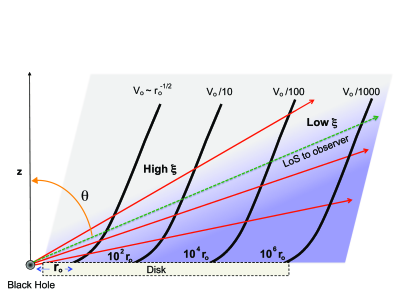
Figure 1: Schematic of an MHD accretion disk wind. Poloidal 2D wind streamlines (thick solid), the decreasing velocity ($v_{0}\approx c$) and ionization ($\xi$) with radius is illustrated. The hatched region represents the absorber of the GRO J1655-40  wind region with 100-1,000 km s^-1. The arrows indicate possible line-of-sight (LoS) effects with the green arrow believed to be the true LoS based on published binary solutions.

Figure 1 Schematic of an MHD accretion disk wind.

Poloidal 2D wind streamlines (thick solid), the decreasing velocity ($v_{0}\approx c$) and ionization ($\xi$) with radius is illustrated. The hatched region represents the absorber of the GRO J1655-40  wind region with 100-1,000 km s^-1. The arrows indicate possible line-of-sight (LoS) effects with the green arrow believed to be the true LoS based on published binary solutions.

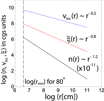
Figure 2: Radial wind profiles inferred from our best-fit model of $\alpha=0.2$. Wind density $n$[cm^-3] (black), the LoS wind velocity $V$ (cm/s) (blue) and the ionization parameter $\xi$ [erg cm s^-1] (red) for $\theta_{\rm obs}=80^{\circ}$. The vertical line indicates the location of the innermost wind streamline for $80^{\circ}$. Note that $\log(n)$ is offset by -11.0 in the vertical direction for presentation purposes.

Figure 2 Radial wind profiles inferred from our best-fit model of $\alpha=0.2$.

Wind density $n$[cm^-3] (black), the LoS wind velocity $V$ (cm/s) (blue) and the ionization parameter $\xi$ [erg cm s^-1] (red) for $\theta_{\rm obs}=80^{\circ}$ and $\alpha=0.2$. The vertical line indicates the location of the innermost wind streamline for $80^{\circ}$. Note that $\log(n)$ is offset by -11.0 in the vertical direction for presentation purposes.

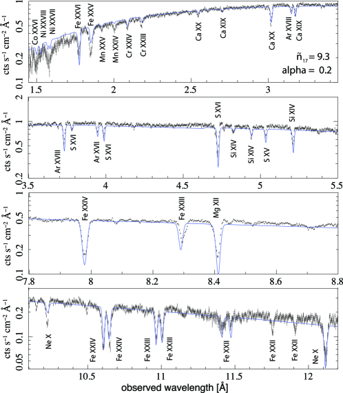
Figure 3: The 46-ks Chandra/HETG spectrum of GRO J1655-40 overlaid on the global MHD-wind model for $\alpha=0.2$ (blue line) with $\tilde{n}_{\rm 17}=9.3$. Adopting the previously constrained baseline continuum (i.e. a multicolor disk model diskbb of $kT=1.35$ keV with $L_{x}=5\times 10^{37}$ erg s^-1), the composite line spectra are computed assuming solar abundances for all ions as discussed in the text and shown in detail in Fig. 4. We find $\theta=80^{\circ}$ and $\tilde{n}_{\rm 17}=9.3$ at $r_{o}=3.81\times 10^{6}$ cm with $M=7M_{\odot}$ black hole for the best-fit spectrum. The best-fit wind parameters are listed in Table 2 in Supplementary Materials.

Figure 3 The 46-ks Chandra/HETG spectrum of GRO J1655-40 overlaid on the global MHD-wind model for $\alpha=0.2$ (blue line) with $\tilde{n}_{\rm 17}=9.3$.

Adopting the previously constrained baseline continuum (i.e. a multicolor disk model diskbb of $kT=1.35$ keV with $L_{x}=5\times 10^{37}$ erg s^-1), the composite line spectra are computed assuming solar abundances for all ions as discussed in the text and shown in detail in Fig. 4. We find $\theta=80^{\circ}$ and $n_{o}=9.3\times 10^{17}$ cm^-3 at $r_{o}=3.81\times 10^{6}$ cm with $M=7M_{\odot}$ black hole for the best-fit spectrum. The best-fit wind parameters are listed in Table 2 in Supplementary Materials.

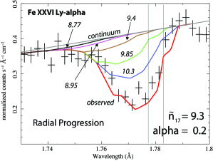
Figure 4: Modeling the Fe xxvi Ly$\alpha$ doublet (1.778, 17834 Å) and the Ne x Ly$\alpha$ doublet (12.132, 12.136 Å) with the MHD winds of $\alpha=0.2$ and $\tilde{n}_{\rm 17}=9.3$. The progressive development of each spectrum with increasing distance $r$ is shown by the sequence of colored lines convolved with the Chandra/HETG resolution and overlaid on the data (the red line corresponds to the line profile as seen at infinity). The profiles were computed employing the values of ($n_{0},\alpha,\theta$) of Figure 3. The double vertical lines denote the rest frame wavelength of these transitions, while the numbers at each colored line denotes the value of $\log r\textmd{[cm]}$ along the LoS. One should note that the model spectra (in color) are not fit to the data but an a priori calculation overlaid on GRO J1655-40 data.

Figure 4 Modeling the Fe xxvi Ly$\alpha$ doublet (1.778, 17834 Å) and the Ne x Ly$\alpha$ doublet (12.132, 12.136 Å) with the MHD winds of $\alpha=0.2$ and $\tilde{n}_{\rm 17}=9.3$.

The progressive development of each spectrum with increasing distance $r$ is shown by the sequence of colored lines convolved with the Chandra/HETG resolution and overlaid on the data (the red line corresponds to the line profile as seen at infinity). The profiles were computed employing the values of ($n_{0},\alpha,\theta$) of Figure 3. The double vertical lines denote the rest frame wavelength of these transitions, while the numbers at each colored line denotes the value of $\log r\textmd{[cm]}$ along the LoS. One should note that the model spectra (in color) are not fit to the data but an a priori calculation overlaid on GRO J1655-40 data.

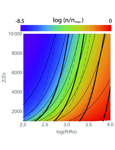
Figure 5: Fig. S1.
A poloidal 2D view of the fiducial MHD-driven disk-wind. . We show the magnetic field lines (thick solid) along with the density distribution $n(r,\theta)$ (in color) and contours (thin solid) and contours of the ionization parameter $\log\xi$ (dashed), as a function of cylindrical distances $(R,Z)$ in units of the innermost launching radius $R_{0}$. Note the $\textmd{linear}(Z)-\log(R)$ character of this Figure, where the line-of-sight (LoS) is not a straight line.

Figure S1. A poloidal 2D view of the fiducial MHD-driven disk-wind.

We show the magnetic field lines (thick solid) along with the density distribution $n(r,\theta)$ (in color) and contours (thin solid) and contours of the ionization parameter $\log\xi$ (dashed), as a function of cylindrical distances $(R,Z)$ in units of the innermost launching radius $R_{0}$. Note the $\textmd{linear}(Z)-\log(R)$ character of this Figure, where the line-of-sight (LoS) is not a straight line.

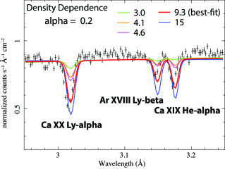
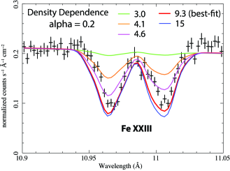
Figure 6: Fig. S2.
Density normalization dependence ($\tilde{n}_{17}$) of specific lines with $\alpha=0.2$. Lines profiles of Ca xx Ly$\alpha$, Ar xviii Ly$\beta$, Ca xix He$\alpha$ and resonant Fe xxiii, as an example, for $\alpha=0.2$ in comparison with Chandra/HETG data with $\tilde{n}_{17}=3.0$ (green), $4.1$ (orange), $4.6$ (magenta), $9.3$ (red; best-fit value) and $15$ (blue). Note that all the lines are uniquely coupled to the same density normalization $n_{0}=\tilde{n}_{\rm 17}10^{17}$ cm^-3 at the launching disk surface. It is demonstrated that the simultaneous modeling for all the observed transition lines with the MHD-wind scenario can clearly differentiate each case and favor the $\alpha=0.2$ wind of $\tilde{n}_{\rm 17}=9.3$.

Figure S2 Density normalization dependence ($\tilde{n}_{17}$) of specific lines with $\alpha=0.2$.

Lines profiles of Ca xx Ly$\alpha$, Ar xviii Ly$\beta$, Ca xix He$\alpha$ and resonant Fe xxiii, as an example, for $\alpha=0.2$ in comparison with Chandra/HETG data with $\tilde{n}_{17}=3.0$ (green), $4.1$ (orange), $4.6$ (magenta), $9.3$ (red; best-fit value) and $15$ (blue). Note that all the lines are uniquely coupled to the same density normalization $n_{0}=\tilde{n}_{\rm 17}10^{17}$ cm^-3 at the launching disk surface. It is demonstrated that the simultaneous modeling for all the observed transition lines with the MHD-wind scenario can clearly differentiate each case and favor the $\alpha=0.2$ wind of $\tilde{n}_{\rm 17}=9.3$.

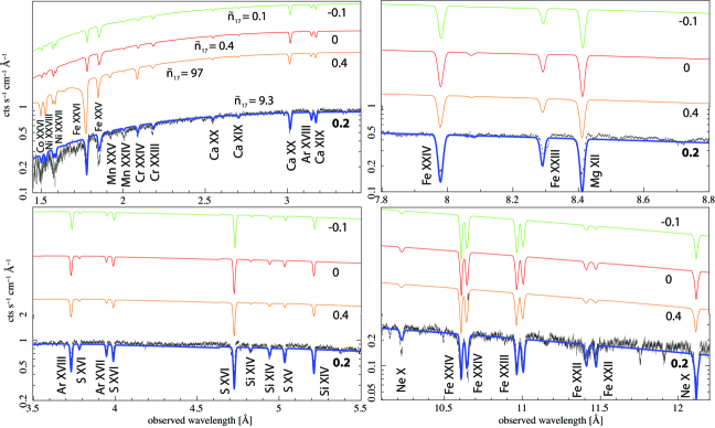
Figure 7: Fig. S3.
The 46-ks Chandra/HETG spectrum of GRO J1655-40  overlaid on different global MHD-wind models of $\alpha=-0.1$ (green), $0$ (red), $0.2$ (blue; best-fit) and $0.4$ (orange). Adopting the same baseline continuum model as in Figure 3, we examined the spectral dependence on wind density profile $\alpha$; $-0.1$ (green), $0$ (red), $0.2$ (blue; best-fit) and $0.4$ (orange) also by varying density normalization $n_{o}$ in each case. Here, we find $\alpha=0.2$ (i.e. $n\propto r^{-1.2}$) to be more consistent with this broad-band data ranging from $\sim 1.5\buildrel{}_{\circ}\over{\mathrm{A}}$ to $\sim 12\buildrel{}_{\circ}\over{\mathrm{A}}$. The overall spectral model components are the same as those in Figures 3 and 4. Note that $\alpha=-0.1,0$ and $0.4$ model spectra are offset by arbitrary factors in flux for presentation purpose.

Figure S3 The 46-ks Chandra/HETG spectrum of GRO J1655-40  overlaid on different global MHD-wind models of $\alpha=-0.1$ (green), $0$ (red), $0.2$ (blue; best-fit) and $0.4$ (orange).

Adopting the same baseline continuum model as in Figure 3, we examined the spectral dependence on wind density profile $\alpha$; $-0.1$ (green), $0$ (red), $0.2$ (blue; best-fit) and $0.4$ (orange) also by varying density normalization $n_{o}$ in each case. Here, we find $\alpha=0.2$ (i.e. $n\propto r^{-1.2}$) to be more consistent with this broad-band data ranging from $\sim 1.5\buildrel{}_{\circ}\over{\mathrm{A}}$ to $\sim 12\buildrel{}_{\circ}\over{\mathrm{A}}$. The overall spectral model components are the same as those in Figures 3 and 4. Note that $\alpha=-0.1,0$ and $0.4$ model spectra are offset by arbitrary factors in flux for presentation purpose.

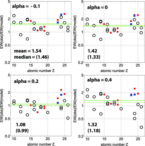
Figure 8: Fig. S4.
EW ratios between our model and data for $\alpha=-0.1,0,0.2$ and 0.4. The ratio, EW(obs)/E(mo), is computed for major ions using models with different $\alpha$ showing its mean (solid green) and median (dotted green) values in each case (also indicated by numbers) to further support the best-fit wind model with $\alpha=0.2$.

Figure S4 EW ratios between our model and data for $\alpha=-0.1,0,0.2$ and 0.4.

The ratio, EW(obs)/E(mo), is computed for major ions using models with different $\alpha$ showing its mean (solid green) and median (dotted green) values in each case (also indicated by numbers) to further support the best-fit wind model with $\alpha=0.2$.

Table S1.
Grids of MHD-Wind Model for GRO J1655-40. Three primary model parameters characterizing the disk-winds for spectral analysis: global density slope $\alpha$ over distance $r$ where $n(r)\propto r^{-(1+\alpha)}$, source inclination angle $\theta$ and plasma number density $\tilde{n}_{17}$ at the footpoint of the MHD wind (i.e. $n_{0}\equiv\tilde{n}_{17}10^{17}$ cm^-3).

Primary Parameter	Range
Density Profile $\alpha$	-0.1, 0, 0.2, 0.4
Viewing Angle $\theta$ (degrees)	$70^{\circ}-80^{\circ}$
Density Normalization factor $\tilde{n}_{17}$	0.024 - 400

Table S2.
Primary best-fit line parameters of the broad-band MHD disk-wind model for GRO J1655-40. For an $\alpha=0.2$ model with $\tilde{n}_{\rm 17}=9.3$, we present the following variables; line energy $E_{o}$ (in keV) and wavelength $\lambda_{o}$ (in $\buildrel{}_{\circ}\over{\mathrm{A}}$) in the source rest-frame, absorber’s characteristic LoS velocity $v_{\rm los}$ (in km s^-1) at the observed trough wavelength, the range of characteristic ionization parameter $\Delta\left(\log\xi_{c}\right)$ corresponding to 50% of the peak differential column density $dN_{\rm ion}/(d\log\xi)$, the corresponding temperature range $\Delta\left(\log T_{c}\right)$, the characteristic line optical depth $\tau_{\rm c}$ at the peak column distance, the modeled line width EW_mo (in m$\buildrel{}_{\circ}\over{\mathrm{A}}$), the hydrogen-equivalent column density $N_{H}$ (in units of $10^{22}$ cm^-2) and the characteristic number density $n_{c}$ (in cm^-3) at the peak column distance.

Transition	$E_{o}$a	$\lambda_{o}$b	$v_{\rm los}$c	$\Delta\left(\log\xi_{c}\right)$	$\Delta\left(\log T_{c}\right)$	$\tau_{c}$	EWmod	$N_{H}$	$\log n_{c}$e
Line	[keV]	[$\buildrel{}_{\circ}\over{\mathrm{A}}$]	[km s-1]	[erg cm s-1]	[K]		[m$\buildrel{}_{\circ}\over{\mathrm{A}}$]	[$10^{\rm 22}$ cm-2]
Fe xxvi Ly$\beta$	8.252	1.5028	320	3.77 - 4.91	6.07 - 6.86	0.854	4.27	28.2	12.2
Ni xxviii Ly$\alpha$	8.102	1.533	831	4.48 - 5.35	6.64 - 6.93	0.216	4.12	69.5	13.3
Cr xxiv Ly$\beta$	7.022	1.7662	2122	4.10 - 5.32	6.32 - 6.93	0.0381	11.9	60.3	12.9
Fe xxvi Ly$\alpha$	6.973	1.7807	328	3.80 - 4.93	6.09 - 6.87	5.14	13.7	30.4	12.3
Fe xxv He$\alpha$	6.700	1.8505	122	3.47 - 4.21	5.93 - 6.42	22.4	10.5	26.6	11.6

Table S2.
Best-Fit Line Parameters of the Broad-Band MHD disk-wind model for GRO J1655-40. Continued.

Transition	$E_{o}$a	$\lambda_{o}$b	$v_{\rm los}$c	$\Delta\left(\log\xi_{c}\right)$	$\Delta\left(\log T_{c}\right)$	$\tau_{\rm max}$	EWmod	$N_{H}$	$\log n_{c}$e
Line	[keV]	[$\buildrel{}_{\circ}\over{\mathrm{A}}$]	[km s-1]	[erg cm s-1]	[K]		[m$\buildrel{}_{\circ}\over{\mathrm{A}}$]	[$10^{\rm 22}$ cm-2]
Fe xxiv Li$\alpha$	6.653	1.8635	1971	3.07 - 3.78	5.81 - 6.07	1.21	10.6	1.96	10.9
Mn xxv Ly$\alpha$	6.442	1.9274	4,068	4.15 - 5.43	6.36 - 6.94	0.0737	3.41	77.5	13.0
Mn xxiv He$\alpha$	6.186	2.006	336	3.31 - 4.15	5.87 - 6.37	0.168	3.14	182	11.4
Cr xxiv Ly$\alpha$	5.932	2.0928	222	4.12 - 5.32	6.34 - 6.93	0.238	5.19	67.1	12.8
Cr xxiii He$\alpha$	5.68	2.1821	117	3.23 - 4.08	5.85 - 6.30	0.415	4.72	9.29	11.3
Ca xix He$\beta$	4.582	2.7054	182	2.57 - 3.42	5.66 - 5.91	0.356	3.42	10.3	10.4
Ca xx Ly$\alpha$	4.107	3.0185	25	3.09 - 4.09	5.81 - 6.30	0.722	7.60	14.1	11.2
Ar xviii Ly$\beta$	3.936	3.1507	190	2.71 - 3.92	5.72 - 6.17	0.289	4.44	5.94	10.8
Ca xix He$\alpha$	3.902	3.1771	80	2.91 - 3.60	5.77 - 5.98	1.60	3.41	1.52	10.6
Ar xviii Ly$\alpha$	3.323	3.7335	185	2.84 - 3.95	5.76 - 6.19	1.62	11.3	9.87	10.9
S xvi Ly$\gamma$	3.276	3.7843	241	2.38 - 3.77	5.48 - 6.07	0.330	4.12	3.40	10.4
Ar xvii He$\alpha$	3.139	3.9493	232	2.73 - 3.41	5.73 - 5.90	2.02	5.86	8.23	10.5
S xvi Ly$\beta$	3.106	3.9913	195	2.39 - 3.77	5.49 - 6.07	0.950	7.04	3.48	10.4
S xvi Ly$\alpha$	2.622	4.730	238	2.58 - 3.83	5.66 - 6.10	5.16	13.9	4.83	10.6
Si xiv Ly$\gamma$	2.506	4.9467	179	2.09 - 3.54	5.19 - 5.96	1.38	5.11	2.15	9.53
S xv He$\alpha$	2.460	5.0387	295	2.44 - 3.24	5.53 - 5.85	8.35	6.58	0.664	10.1

Table S2.
Best-Fit Line Parameters of the Broad-Band MHD disk-wind model for GRO J1655-40. Continued.

Transition	$E_{o}$a	$\lambda_{o}$b	$v_{\rm los}$c	$\Delta\left(\log\xi_{c}\right)$	$\Delta\left(\log T_{c}\right)$	$\tau_{c}$	EWmod	$N_{H}$	$\log n_{c}$e
Line	[keV]	[$\buildrel{}_{\circ}\over{\mathrm{A}}$]	[km s-1]	[erg cm s-1]	[K]		[m$\buildrel{}_{\circ}\over{\mathrm{A}}$]	[$10^{\rm 22}$ cm-2]
Si xiv Ly$\beta$	2.376	5.2173	206	2.09 - 3.55	5.19 - 5.96	3.98	9.29	2.20	12.5
Si xiv Ly$\alpha$	2.006	6.1831	453	2.24 - 3.68	5.35 - 6.03	10.6	19.2	6.54	13.2
Mg xii Ly$\beta$	1.745	7.1063	321	1.88 - 2.85	5.09 - 5.77	5.57	9.62	1.39	12.2
Fe xxiii	1.493	8.3001	319	2.67 - 3.27	5.71 - 5.86	7.47	11.7	1.21	11.7
Mg xii Ly$\alpha$	1.472	8.4219	379	2.00 - 3.27	5.14 - 5.86	32.2	18.3	6.57	12.9
Ne x Ly$\beta$	1.211	10.238	358	1.63 - 2.46	4.86 - 5.56	6.64	8.70	0.901	11.9
Ne x Ly$\alpha$	1.022	12.134	513	1.77 - 2.54	5.00 - 5.64	36.6	21.2	1.42	12.6

^a Rest-frame energy in keV. ^b Rest-frame wavelength in $\buildrel{}_{\circ}\over{\mathrm{A}}$. ^c Line-of-sight (LoS) wind velocity in km s^-1. ^d Model EW value.

^e Wind number density in cm^-3.

References

- [1] Crenshaw, D. M., Kraemer, S. B. & George, I. M. Mass Loss from the Nuclei of Active Galaxies ARA&A 41, 117–167 (2003)
- [2] Behar, E. et al. A Long Look at NGC 3783 with the XMM-Newton Reflection Grating Spectrometer. Astrophys.J. 598, 232-241 (2003).
- [3] Tombesi, F. et al. Evidence for ultra-fast outflows in radio-quiet AGNs. I. Detection and statistical incidence of Fe K-shell absorption lines. A&A 521, 57-92 (2010).
- [4] Holczer, T., Behar, E. & Kaspi, S. Absorption Measure Distribution of the Outflow in IRAS 13349+2438: Direct Observation of Thermal Instability? Astrophys. J. 663, 799-807
- [5] Fukumura, K., Kazanas, D., Contopoulos, I. & Behar, E. Magnetohydrodynamic Accretion Disk Winds as X-ray Absorbers in Active Galactic Nuclei. Astrophys. J. 715, 636-650 (2010)
- [6] Fukumura, K., Kazanas, D., Contopoulos, I. & Behar, E. Modeling High-velocity QSO Absorbers with Photoionized Magnetohydrodynamic Disk Winds. Astrophys. J. Lett. 723, L228-L232 (2010).
- [7] Miller, J. M. et al. The magnetic nature of disk accretion onto black holes. Nature 441, 953-955 (2006)
- [8] Blandford, R. D. & Begelman, M. C. On the fate of gas accreting at a low rate on to a black hole. MNRAS 333, 12–16, (1999).
- [9] Tombesi, F. et al. Wind from the black-hole accretion disk driving a molecular outflow in an active galaxy. Nature 519, 436-438 (2015)
- [10] Begelman, M. C., McKee, C. F. & Shields, G. A. Compton heated winds and coronae above accretion disks. I Dynamics. Astrophys. J. 270, 70-88 (1983).
- [11] Murray, N. et al. Accretion Disk Winds from Active Galactic Nuclei Astrophys. J. 451, 498 (1995)
- [12] Blandford, R. D. & Payne D. G. Hydromagnetic flows from accretion discs and the production of radio jets. Mon. Not. R. Astron. Soc 199, 883-903 (1982).
- [13] Contopoulos, J. & Lovelace,R. V. E. Magnetically driven jets and winds: Exact solutions. Astrophys. J. 429, 139-152 (1994).
- [14] Contopoulos, J. A Simple Type of Magnetically Driven Jets: an Astrophysical Plasma Gun. Astrophys. J. 429, 616-627 (1995)
- [15] Ferreira, J. Magnetically-driven jets from Keplerian accretion discs, A&A 319, 340-359 (1997)
- [16] Miller, J. M. et al. The Accretion Disk Wind in the Black Hole GRO J1655-40. Astrophys. J. 680, 1356 (2008).
- [17] Kallman, T. R. et al. Spectrum synthesis modeling of the X-ray spectrum of GRO J1655-40 taken during the 2000 outburst. Astrophys.J. 701, 865-884 (2009)
- [18] Luketic, S., Proga, D., Kallman, T. R., Raymond, J. C. & Miller, J. M. On the Properties of Thermal Disk Winds in X-ray Transient Sources: A Case Study of GRO J1655-40. Astrophys. J. 719, 515–522 (2010).
- [19] Fukumura, K., Tombesi, F., Kazanas, D., Shrader, C., Behar, E. & Contopoulos, I. Magnetically Driven Accretion Disk Winds and Ultra-fast Outflows in PG 1211+143. Astrophys. J. 805, 17-27 (2015).
- [20] Kazanas, D., Fukumura, K., Behar, E., Contopoulos, I. & Shrader, C. Toward a Unified AGN Structure. Astronom. Rev. 7, No. 3, 92-123 (2012).
- [21] Shidatsu, M., Done, C., & Ueda, Y. An Optically Thick Disk Wind in GRO J1655 40? Astrophys. J. 823, 159-171 (2016)
- [22] Neilsen, J., Rahoui, F., Homan, J., & Buxton, M. A Super-Eddington, Compton-thick Wind in GRO J1655-40? Astrophys. J., 822, 20-34 (2016)
- [23] Netzer, H. A Thermal Wind Model for the X-Ray Outflow in GRO J1655-40. Astrophys. J. Lett., 652, L117-L120 (2006)
- [24] Castor, J. I., Abbot, D. C. & Klein, R. I. Radiation-driven winds in Of stars. Astrophys. J 195, 157-174 (1975).
- [25] Proga, D., Stone, J. M. & Kallman, T. R. Dynamics of line-driven winds in active galactic nuclei. Astrophys. J. 543, 686-696 (2000).
- [26] Behar, E. Density Profiles in Seyfert Outflows. Astrophys.J. 703, 1346-1351 (2009).
- [27] Miller, J. M. et al. Powerful, Rotating Disk Winds from Stellar-mass Black Holes. Astrophys.J. 814, 87–114 (2015)
- [28] Kallman, T. R & Bautista, M. A. Photoionzation and High Density Gas. Astrophys. J. Suppl. 133, 221-253 (2001).
- [29] Neilsen, J. & Lee, J. C. Accretion disk winds as the jet suppression mechanism in the microquasar GRS 1915+105. Nature 458, 481-485 (2009).

References

- [1]
- [2] Hjellming, R. M. & Rupen, M. P. Episodic ejection of relativistic jets by the X-ray transient GRO J1655-40. Nature. 375, 464-468 (1995)
- [3] Dickey, J. M. & Lockman, F. J. H I in the Galaxy. Annu. Rev. Astron. Astr. 28, 215-261 (1990)
- [4] Blustin, A. J., Page, M. J., Fuerst, S. V., Branduardi-Raymont, G. & Ashton, C. E. The nature and origin of Seyfert warm absorbers. Astron. & Astrophys. 431, 111-125 (2005)
- [5] George, I. M., Turner, T. J., Netzer, H., Nandra, K., Mushotzky, R. F. & Yaqoob, T. ASCA Observations of Seyfert 1 Galaxies. III. The Evidence for Absorption and Emission Due to Photoionized Gas. Astrophys. J. Suppl. 114, 73-120 (1998)
- [6] McKernan, B., Yaqoob, T. & Reynolds, C. S. A soft X-ray study of type I active galactic nuclei observed with Chandra high-energy transmission grating spectrometer. Astrophys. J. Suppl. 379, 1359-1372 (2007)
- [7] Chartas, G., Saez, C., Brandt, W. N., Giustini, M., & Garmire, G. P. Confirmation of and Variable Energy Injection by a Near-Relativistic Outflow in APM 08279+5255. Astrophys. J. 706, 644-656 (2009)
- [8] Schurch, N. J. & Done, C. The impact of accretion disc winds on the X-ray spectrum of AGN - I. XSCORT. Mon. Not. R. Astron. Soc. 381, 1413-1425 (2007)
- [9] Sim, S. A., Long, K. S., Miller, L. & Turner, T. J. Multidimensional modelling of X-ray spectra for AGN accretion disc outflows. Mon. Not. R. Astron. Soc. 388, 611-624 (2008)
- [10] Mihalas, D. Stellar Atmospheres. (W. H. Freeman and Co.) 650p. (1978)
- [11] Crenshaw, D. M. & Kraemer, S. B. Feedback from Mass Outflows in Nearby Active Galactic Nuclei. I. Ultraviolet and X-Ray Absorbers. Astrophys. J. 753, 75-85 (2012)
- [12] Chakravorty, S. et al. Absorption lines from magnetically driven winds in X-ray binaries. Astron. & Astrophys. 589, A119-135 (2016)
- [13] Laha, S. et al. Warm absorbers in X-rays (WAX), a comprehensive high-resolution grating spectral study of a sample of Seyfert galaxies - I. A global view and frequency of occurrence of warm absorbers. Mon. Not. R. Astron. Soc., 441, 2613-2643 (2014)
- [14] King, A. L. et al. Regulation of black hole winds and jets across the mass scale. Astrophys. J., 762, 103-121 (2013)
- [15] Neilsen, J. & Homan, J. A Hybrid Magnetically/Thermally Driven Wind in the Black Hole GRO J1655-40? Astrophys. J., 750, 27-35 (2012)