1 Introduction
The study of optimal stopping of Brownian motion
as close as possible to its ultimate maximum has
been initiated in Graversen, Peskir and Shiryaev [3 ] .
For geometric Brownian motion, the optimal prediction problem
V t = inf t ≤ τ ≤ T IE [ sup 0 ≤ s ≤ T Y s Y τ | ℱ t 0 ] subscript 𝑉 𝑡 subscript infimum 𝑡 𝜏 𝑇 IE delimited-[] conditional subscript supremum 0 𝑠 𝑇 subscript 𝑌 𝑠 subscript 𝑌 𝜏 subscript superscript ℱ 0 𝑡 V_{t}=\inf\limits_{t\leq\tau\leq T}\mathop{\hbox{\rm I\kern-1.99997ptE}}\nolimits\left[\sup\limits_{0\leq s\leq T}\frac{Y_{s}}{Y_{\tau}}\Big{|}{\cal F}^{0}_{t}\right] (1.1)
of selling at the ultimate maximum
over all ( ℱ s t ) s ∈ [ t , T ] subscript subscript superscript ℱ 𝑡 𝑠 𝑠 𝑡 𝑇 ({\cal F}^{t}_{s})_{s\in[t,T]} τ ∈ [ t , T ] 𝜏 𝑡 𝑇 \tau\in[t,T] [2 ] by Du Toit and Peskir
when the asset price ( Y t ) t ∈ IR + subscript subscript 𝑌 𝑡 𝑡 subscript IR (Y_{t})_{t\in{\mathord{{\rm I\kern-3.0ptR}}}_{+}} ( ℱ s t ) s ∈ [ t , T ] subscript subscript superscript ℱ 𝑡 𝑠 𝑠 𝑡 𝑇 ({\cal F}^{t}_{s})_{s\in[t,T]} ( B s − B t ) s ∈ [ t , T ] subscript subscript 𝐵 𝑠 subscript 𝐵 𝑡 𝑠 𝑡 𝑇 (B_{s}-B_{t})_{s\in[t,T]} [10 ] for background on optimal stopping and
free boundary problems, and Chapter VIII therein for ultimate
position and maximum problems.
This framework has recently been
extended in Liu and Privault [7 ]
to the regime-switching model
d Y t = μ ( β t ) Y t d t + σ ( β t ) Y t d B t , 0 ≤ t ≤ T , formulae-sequence 𝑑 subscript 𝑌 𝑡 𝜇 subscript 𝛽 𝑡 subscript 𝑌 𝑡 𝑑 𝑡 𝜎 subscript 𝛽 𝑡 subscript 𝑌 𝑡 𝑑 subscript 𝐵 𝑡 0 𝑡 𝑇 dY_{t}=\mu(\beta_{t})Y_{t}dt+\sigma(\beta_{t})Y_{t}dB_{t},\qquad 0\leq t\leq T, (1.2)
driven by a finite-state, observable continuous-time Markov chain
( β t ) t ∈ IR + subscript subscript 𝛽 𝑡 𝑡 subscript IR (\beta_{t})_{t\in{\mathord{{\rm I\kern-3.0ptR}}}_{+}} ℳ := { 1 , 2 , … , m } assign ℳ 1 2 … 𝑚 {\cal M}:=\{1,2,\ldots,m\} ( B t ) t ∈ IR + subscript subscript 𝐵 𝑡 𝑡 subscript IR (B_{t})_{t\in{\mathord{{\rm I\kern-3.0ptR}}}_{+}} ( Ω , ( ℱ t ) t ∈ IR + , ℙ ) Ω subscript subscript ℱ 𝑡 𝑡 subscript IR ℙ (\Omega,({\cal F}_{t})_{t\in{\mathord{{\rm I\kern-3.0ptR}}}_{+}},{\mathord{\mathbb{P}}}) ( ℱ t ) t ∈ IR + subscript subscript ℱ 𝑡 𝑡 subscript IR ({\cal F}_{t})_{t\in{\mathord{{\rm I\kern-3.0ptR}}}_{+}} ( B t ) t ∈ IR + subscript subscript 𝐵 𝑡 𝑡 subscript IR (B_{t})_{t\in{\mathord{{\rm I\kern-3.0ptR}}}_{+}} ( β t ) t ∈ IR + subscript subscript 𝛽 𝑡 𝑡 subscript IR (\beta_{t})_{t\in{\mathord{{\rm I\kern-3.0ptR}}}_{+}} μ : ℳ ⟶ IR : 𝜇 ⟶ ℳ IR \mu:{\cal M}\longrightarrow{\mathord{{\rm I\kern-3.0ptR}}} σ : ℳ ⟶ ( 0 , ∞ ) : 𝜎 ⟶ ℳ 0 \sigma:{\cal M}\longrightarrow(0,\infty)
Regime-switching models were introduced by Hamilton [5 ]
in the framework of time series,
in order to model the influence of external market factors.
European options have been priced
in continuous time regime-switching models
by Yao, Zhang and Zhou [12 ]
using a successive approximation algorithm.
Optimal stopping for option pricing
with regime switching has been dealt with in e.g.
Guo [4 ]
and Le and Wang [6 ] .
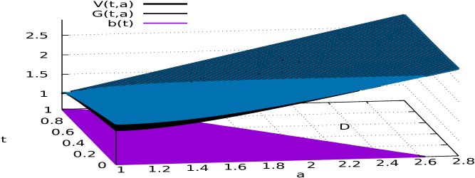
It has been shown in particular in [2 ] that
the boundary function b ( t ) 𝑏 𝑡 b(t) t ∈ [ 0 , T ] 𝑡 0 𝑇 t\in[0,T]
G ( t , b ( t ) ) = J ( t , b ( t ) ) − ∫ t T K ( t , r , b ( t ) ) 𝑑 r , 𝐺 𝑡 𝑏 𝑡 𝐽 𝑡 𝑏 𝑡 superscript subscript 𝑡 𝑇 𝐾 𝑡 𝑟 𝑏 𝑡 differential-d 𝑟 G(t,b(t))=J(t,b(t))-\int_{t}^{T}K(t,r,b(t))dr, (1.3)
0 ≤ t ≤ T 0 𝑡 𝑇 0\leq t\leq T b ( T ) 𝑏 𝑇 b(T) J ( t , x ) 𝐽 𝑡 𝑥 J(t,x) K ( t , r , x ) 𝐾 𝑡 𝑟 𝑥 K(t,r,x) [2 ] .
Under regime switching, the optimal boundary functions
depend on the regime state of the system, and they may not be monotone
if the drift coefficients ( μ ( i ) ) i ∈ ℳ subscript 𝜇 𝑖 𝑖 ℳ (\mu(i))_{i\in{\cal M}} 3 4 5 [8 ] and
[9 ] for other optimal settings that involve
non monotone boundary functions.
In the regime switching setting however,
no Volterra equation such as (1.3 [7 ] .
In addition, the free boundary problem in the regime switching
case consists in a system of interacting PDEs, making its direct
solution more difficult, cf. Proposition 5.2 in [7 ] .
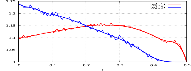
In Buffington and Elliott [1 ]
a free boundary problem has been solved
under an ordering assumption
on the boundary functions in the two-state case,
see Assumption 3.1 therein,
however this condition may not hold in general in our setting,
cf. Figure 4
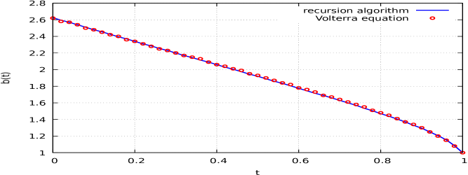
In this paper we construct a recursive
algorithm for the numerical solution of (1.1 1.2 ( μ ( i ) ) i ∈ ℳ subscript 𝜇 𝑖 𝑖 ℳ (\mu(i))_{i\in{\cal M}} O ( n ) 𝑂 𝑛 O(n) n 𝑛 n O ( n 2 ) 𝑂 superscript 𝑛 2 O(n^{2}) 1.3 5
We start by recalling the main results of [7 ] .
From Lemma 2.1 in
[7 ] ,
the optimal value function V t subscript 𝑉 𝑡 V_{t} 1.1
V t = V ( t , Y ^ 0 , t / Y t , β t ) , subscript 𝑉 𝑡 𝑉 𝑡 subscript ^ 𝑌 0 𝑡
subscript 𝑌 𝑡 subscript 𝛽 𝑡 V_{t}=V(t,\hat{Y}_{0,t}/Y_{t},\beta_{t}),
where the function
V : [ 0 , T ] × [ 1 , ∞ ) × ℳ → IR + : 𝑉 → 0 𝑇 1 ℳ subscript IR V:[0,T]\times[1,\infty)\times{\cal M}\rightarrow{\mathord{{\rm I\kern-3.0ptR}}}_{+}
V ( t , a , j ) 𝑉 𝑡 𝑎 𝑗 \displaystyle V(t,a,j) := assign \displaystyle:= inf t ≤ τ ≤ T IE [ 1 Y τ max ( a Y t , Y ^ t , T ) | β t = j ] subscript infimum 𝑡 𝜏 𝑇 IE delimited-[] conditional 1 subscript 𝑌 𝜏 𝑎 subscript 𝑌 𝑡 subscript ^ 𝑌 𝑡 𝑇
subscript 𝛽 𝑡 𝑗 \displaystyle\inf\limits_{t\leq\tau\leq T}\mathop{\hbox{\rm I\kern-1.99997ptE}}\nolimits\left[\frac{1}{{Y_{\tau}}}\max(aY_{t},\hat{Y}_{t,T})\;\Big{|}\;\beta_{t}=j\right] (1.4)
= \displaystyle= inf t ≤ τ ≤ T IE [ G ( τ , β τ , 1 Y τ max ( a Y t , Y ^ t , τ ) ) | β t = j ] , subscript infimum 𝑡 𝜏 𝑇 IE delimited-[] conditional 𝐺 𝜏 subscript 𝛽 𝜏 1 subscript 𝑌 𝜏 𝑎 subscript 𝑌 𝑡 subscript ^ 𝑌 𝑡 𝜏
subscript 𝛽 𝑡 𝑗 \displaystyle\inf_{t\leq\tau\leq T}\mathop{\hbox{\rm I\kern-1.99997ptE}}\nolimits\left[G\left(\tau,\beta_{\tau},\frac{1}{Y_{\tau}}\max\left(aY_{t},\hat{Y}_{t,\tau}\right)\right)\;\Big{|}\;\beta_{t}=j\right], (1.5)
for t ∈ [ 0 , T ] 𝑡 0 𝑇 t\in[0,T] j ∈ ℳ 𝑗 ℳ j\in{\cal M} a ≥ 1 𝑎 1 a\geq 1 Y ^ s , t := max r ∈ [ s , t ] Y r assign subscript ^ 𝑌 𝑠 𝑡
subscript 𝑟 𝑠 𝑡 subscript 𝑌 𝑟 \hat{Y}_{s,t}:=\max_{r\in[s,t]}Y_{r} 0 ≤ s ≤ t ≤ T 0 𝑠 𝑡 𝑇 0\leq s\leq t\leq T
G ( t , a , j ) := IE [ max ( a , Y ^ t , T / Y t ) | β t = j ] , t ∈ [ 0 , T ] , j ∈ ℳ . formulae-sequence assign 𝐺 𝑡 𝑎 𝑗 IE delimited-[] conditional 𝑎 subscript ^ 𝑌 𝑡 𝑇
subscript 𝑌 𝑡 subscript 𝛽 𝑡 𝑗 formulae-sequence 𝑡 0 𝑇 𝑗 ℳ G(t,a,j):=\mathop{\hbox{\rm I\kern-1.99997ptE}}\nolimits\left[\max\left(a,\hat{Y}_{t,T}/Y_{t}\right)\;\Big{|}\;\beta_{t}=j\right],\quad t\in[0,T],\ j\in{\cal M}. (1.6)
Here, the infimum
is taken over all ( ℱ s t ) s ∈ [ t , T ] subscript superscript subscript ℱ 𝑠 𝑡 𝑠 𝑡 𝑇 ({\cal F}_{s}^{t})_{s\in[t,T]} τ 𝜏 \tau ℱ s t := σ ( B r − B t , β r : t ≤ r ≤ s ) {\cal F}_{s}^{t}:=\sigma(B_{r}-B_{t},\ \beta_{r}\ :\ t\leq r\leq s) s ∈ [ t , T ] 𝑠 𝑡 𝑇 s\in[t,T] [7 ] ,
given β t = j ∈ ℳ subscript 𝛽 𝑡 𝑗 ℳ \beta_{t}=j\in{\cal M} Y ^ 0 , t / Y t = a ∈ [ 1 , ∞ ) subscript ^ 𝑌 0 𝑡
subscript 𝑌 𝑡 𝑎 1 {\hat{Y}_{0,t}}/{Y_{t}}=a\in[1,\infty) t ∈ [ 0 , T ] 𝑡 0 𝑇 t\in[0,T] 1.1 1.5
τ D ( t , a , j ) := inf { r ≥ t : ( r , Y ^ 0 , r Y r , β r ) ∈ D } assign subscript 𝜏 𝐷 𝑡 𝑎 𝑗 infimum conditional-set 𝑟 𝑡 𝑟 subscript ^ 𝑌 0 𝑟
subscript 𝑌 𝑟 subscript 𝛽 𝑟 𝐷 \tau_{D}(t,a,j):=\inf\left\{r\geq t\ :\;\left(r,\frac{\hat{Y}_{0,r}}{Y_{r}},\beta_{r}\right)\in D\right\}
of the stopping set
D := { ( t , a , j ) ∈ [ 0 , T ] × [ 1 , ∞ ) × ℳ : V ( t , a , j ) = G ( t , a , j ) } assign 𝐷 conditional-set 𝑡 𝑎 𝑗 0 𝑇 1 ℳ 𝑉 𝑡 𝑎 𝑗 𝐺 𝑡 𝑎 𝑗 D:=\big{\{}(t,a,j)\in[0,T]\times[1,\infty)\times{\cal M}\ :\ V(t,a,j)=G(t,a,j)\big{\}} (1.7)
by the process ( r , Y ^ 0 , r / Y r , β r ) r ∈ [ t , T ] subscript 𝑟 subscript ^ 𝑌 0 𝑟
subscript 𝑌 𝑟 subscript 𝛽 𝑟 𝑟 𝑡 𝑇 (r,\hat{Y}_{0,r}/Y_{r},\beta_{r})_{r\in[t,T]}
The stopping set D 𝐷 D 1.7
D = { ( t , y , j ) ∈ [ 0 , T ] × [ 1 , ∞ ) × ℳ : y ≥ b D ( t , j ) } 𝐷 conditional-set 𝑡 𝑦 𝑗 0 𝑇 1 ℳ 𝑦 subscript 𝑏 𝐷 𝑡 𝑗 D=\left\{(t,y,j)\in[0,T]\times[1,\infty)\times{\cal M}\ :\ y\geq b_{D}(t,j)\right\}
in terms of the boundary functions b D ( t , j ) subscript 𝑏 𝐷 𝑡 𝑗 b_{D}(t,j)
b D ( t , j ) := inf { x ∈ [ 1 , ∞ ) : ( t , x , j ) ∈ D } , t ∈ [ 0 , T ] , j ∈ ℳ , formulae-sequence assign subscript 𝑏 𝐷 𝑡 𝑗 infimum conditional-set 𝑥 1 𝑡 𝑥 𝑗 𝐷 formulae-sequence 𝑡 0 𝑇 𝑗 ℳ b_{D}(t,j):=\inf\{x\in[1,\infty)\ :\ (t,x,j)\in D\},\qquad t\in[0,T],\quad j\in{\cal M},
cf. Proposition 3.2 of [7 ] .
If the condition μ ( j ) ≥ 0 𝜇 𝑗 0 \mu(j)\geq 0 j ∈ ℳ 𝑗 ℳ j\in{\cal M} t ↦ b D ( t , j ) maps-to 𝑡 subscript 𝑏 𝐷 𝑡 𝑗 t\mapsto b_{D}(t,j) 4 μ ( j ) ≤ 0 𝜇 𝑗 0 \mu(j)\leq 0 j ∈ ℳ 𝑗 ℳ j\in{\cal M} b D ( t , j ) = 1 subscript 𝑏 𝐷 𝑡 𝑗 1 b_{D}(t,j)=1 t ∈ [ 0 , T ] 𝑡 0 𝑇 t\in[0,T] j ∈ ℳ 𝑗 ℳ j\in{\cal M} [7 ] .
In this paper we construct a recursive algorithm for
the numerical solution of the optimal stopping problem
(1.1 D 𝐷 D V ( t , a , j ) 𝑉 𝑡 𝑎 𝑗 V(t,a,j) G ( t , a , j ) 𝐺 𝑡 𝑎 𝑗 G(t,a,j) 2.1 4.1 1.3 b D ( t , j ) subscript 𝑏 𝐷 𝑡 𝑗 b_{D}(t,j) μ ( j ) ≥ 0 𝜇 𝑗 0 \mu(j)\geq 0 j ∈ ℳ 𝑗 ℳ j\in{\cal M} [7 ] ,
cf. for example Figure 4 [2 ]
as they are no longer available in the regime-switching
setting.
Our algorithm extends the method of [12 ]
as it applies not only to the computation of expectations,
but also to optimal stopping problems.
However it differs from [12 ] , even when restricted to
expectations IE [ ϕ ( Y T ) ] IE delimited-[] italic-ϕ subscript 𝑌 𝑇 \mathop{\hbox{\rm I\kern-1.99997ptE}}\nolimits[\phi(Y_{T})] ϕ ( Y T ) italic-ϕ subscript 𝑌 𝑇 \phi(Y_{T}) ( Y t ) t ∈ [ 0 , T ] subscript subscript 𝑌 𝑡 𝑡 0 𝑇 (Y_{t})_{t\in[0,T]} 1.2 [12 ]
is based on the jump times of the Markov chain ( β t ) t ∈ IR + subscript subscript 𝛽 𝑡 𝑡 subscript IR (\beta_{t})_{t\in{\mathord{{\rm I\kern-3.0ptR}}}_{+}} [ 0 , T ] 0 𝑇 [0,T] 2.3
2 Main results
In the sequel we let δ n := T / n assign subscript 𝛿 𝑛 𝑇 𝑛 \delta_{n}:=T/n t k n := k δ n assign subscript superscript 𝑡 𝑛 𝑘 𝑘 subscript 𝛿 𝑛 t^{n}_{k}:=k\delta_{n} k = 0 , 1 , … , n 𝑘 0 1 … 𝑛
k=0,1,\ldots,n 𝒯 n := ( t 0 n , t 1 n , … , t n n ) assign subscript 𝒯 𝑛 subscript superscript 𝑡 𝑛 0 subscript superscript 𝑡 𝑛 1 … subscript superscript 𝑡 𝑛 𝑛 {\cal T}_{n}:=(t^{n}_{0},t^{n}_{1},\ldots,t^{n}_{n})
⌈ s ⌉ n := min { t ∈ 𝒯 n : t ≥ s } , s ∈ [ 0 , T ] , n ≥ 1 . formulae-sequence assign subscript 𝑠 𝑛 : 𝑡 subscript 𝒯 𝑛 𝑡 𝑠 formulae-sequence 𝑠 0 𝑇 𝑛 1 \lceil s\rceil_{n}:=\min\big{\{}t\in{\cal T}_{n}\ :\ t\geq s\big{\}},\quad s\in[0,T],\quad n\geq 1.
In the following Theorem 2.1 3 V n ( t , a , j ) subscript 𝑉 𝑛 𝑡 𝑎 𝑗 V_{n}(t,a,j) 2.3 T 𝑇 T
Theorem 2.1
( i ) 𝑖 (i) For all
t ∈ [ 0 , T ] 𝑡 0 𝑇 t\in[0,T] , j = 1 , 2 , … , m 𝑗 1 2 … 𝑚
j=1,2,\ldots,m and a ≥ 1 𝑎 1 a\geq 1 , the solution V ( t , a , j ) 𝑉 𝑡 𝑎 𝑗 V(t,a,j) of ( 1.4 ) satisfies
V ( t , a , j ) = lim n → ∞ V n ( ⌈ t ⌉ n , a , j ) , 𝑉 𝑡 𝑎 𝑗 subscript → 𝑛 subscript 𝑉 𝑛 subscript 𝑡 𝑛 𝑎 𝑗 V(t,a,j)=\lim\limits_{n\rightarrow\infty}V_{n}(\lceil t\rceil_{n},a,j), (2.1)
where V n ( t k n , a , j ) subscript 𝑉 𝑛 subscript superscript 𝑡 𝑛 𝑘 𝑎 𝑗 V_{n}(t^{n}_{k},a,j) is the discrete infimum
V n ( t k n , a , j ) := inf t k + 1 n ≤ τ n ≤ T IE [ Y ^ 0 , T Y τ n | Y ^ 0 , t k n Y t k n = a , β t k n = j ] , k = 0 , 1 , … , n − 1 , formulae-sequence assign subscript 𝑉 𝑛 subscript superscript 𝑡 𝑛 𝑘 𝑎 𝑗 subscript infimum subscript superscript 𝑡 𝑛 𝑘 1 subscript 𝜏 𝑛 𝑇 IE delimited-[] formulae-sequence conditional subscript ^ 𝑌 0 𝑇
subscript 𝑌 subscript 𝜏 𝑛 subscript ^ 𝑌 0 subscript superscript 𝑡 𝑛 𝑘
subscript 𝑌 subscript superscript 𝑡 𝑛 𝑘 𝑎 subscript 𝛽 subscript superscript 𝑡 𝑛 𝑘 𝑗 𝑘 0 1 … 𝑛 1
V_{n}(t^{n}_{k},a,j):=\inf\limits_{t^{n}_{k+1}\leq\tau_{n}\leq T}\mathop{\hbox{\rm I\kern-1.99997ptE}}\nolimits\left[\frac{\hat{Y}_{0,T}}{Y_{\tau_{n}}}\;\Big{|}\;\frac{\hat{Y}_{0,t^{n}_{k}}}{Y_{t^{n}_{k}}}=a,\ \beta_{t^{n}_{k}}=j\right],\quad k=0,1,\ldots,n-1, (2.2)
taken over all
𝒯 n subscript 𝒯 𝑛 {\cal T}_{n} -valued
stopping times τ n subscript 𝜏 𝑛 \tau_{n} , and
V n ( T , a , j ) := V ( T , a , j ) = a assign subscript 𝑉 𝑛 𝑇 𝑎 𝑗 𝑉 𝑇 𝑎 𝑗 𝑎 V_{n}(T,a,j):=V(T,a,j)=a .
( i i ) 𝑖 𝑖 (ii)
The value of V n ( t k n , a , j ) subscript 𝑉 𝑛 subscript superscript 𝑡 𝑛 𝑘 𝑎 𝑗 V_{n}(t^{n}_{k},a,j) in ( 2.2 ) can be computed by
the backward induction
V n ( t k − 1 n , a , j ) = subscript 𝑉 𝑛 subscript superscript 𝑡 𝑛 𝑘 1 𝑎 𝑗 absent \displaystyle V_{n}\left(t^{n}_{k-1},a,j\right)= IE [ G ( t k n , Y ^ 0 , t k n Y t k n , β t k n ) ∧ V n ( t k n , Y ^ 0 , t k n Y t k n , β t k n ) | Y ^ 0 , t k − 1 n Y t k − 1 n = a , β t k − 1 n = j ] , IE delimited-[] formulae-sequence 𝐺 subscript superscript 𝑡 𝑛 𝑘 subscript ^ 𝑌 0 subscript superscript 𝑡 𝑛 𝑘
subscript 𝑌 subscript superscript 𝑡 𝑛 𝑘 subscript 𝛽 subscript superscript 𝑡 𝑛 𝑘 conditional subscript 𝑉 𝑛 subscript superscript 𝑡 𝑛 𝑘 subscript ^ 𝑌 0 subscript superscript 𝑡 𝑛 𝑘
subscript 𝑌 subscript superscript 𝑡 𝑛 𝑘 subscript 𝛽 subscript superscript 𝑡 𝑛 𝑘 subscript ^ 𝑌 0 subscript superscript 𝑡 𝑛 𝑘 1
subscript 𝑌 subscript superscript 𝑡 𝑛 𝑘 1 𝑎 subscript 𝛽 subscript superscript 𝑡 𝑛 𝑘 1 𝑗 \displaystyle\mathop{\hbox{\rm I\kern-1.99997ptE}}\nolimits\left[G\left(t^{n}_{k},\frac{\hat{Y}_{0,t^{n}_{k}}}{Y_{t^{n}_{k}}},\beta_{t^{n}_{k}}\right)\wedge V_{n}\left(t^{n}_{k},\frac{\hat{Y}_{0,t^{n}_{k}}}{Y_{t^{n}_{k}}},\beta_{t^{n}_{k}}\right)\;\Big{|}\;\frac{\hat{Y}_{0,t^{n}_{k-1}}}{Y_{t^{n}_{k-1}}}=a,\ \beta_{t^{n}_{k-1}}=j\right], (2.3)
for k = 1 , 2 , … , n 𝑘 1 2 … 𝑛
k=1,2,\ldots,n ,
under the terminal condition V n ( T , a , j ) = G ( T , a , j ) = a subscript 𝑉 𝑛 𝑇 𝑎 𝑗 𝐺 𝑇 𝑎 𝑗 𝑎 V_{n}(T,a,j)=G(T,a,j)=a , a ≥ 1 𝑎 1 a\geq 1 ,
where G ( t , a , j ) 𝐺 𝑡 𝑎 𝑗 G(t,a,j) in defined in ( 1.6 ).
In addition, by the following Theorem 2.2 4 G ( t , a , j ) 𝐺 𝑡 𝑎 𝑗 G(t,a,j) 2.3
φ r ( x , y ) := 2 π ( 2 y − x ) r 3 / 2 e − ( 2 y − x ) 2 / 2 r , 0 ≤ x ≤ y , r ∈ ( 0 , T ] , formulae-sequence formulae-sequence assign subscript 𝜑 𝑟 𝑥 𝑦 2 𝜋 2 𝑦 𝑥 superscript 𝑟 3 2 superscript 𝑒 superscript 2 𝑦 𝑥 2 2 𝑟 0 𝑥 𝑦 𝑟 0 𝑇 \varphi_{r}(x,y):=\sqrt{\frac{2}{\pi}}\frac{(2y-x)}{r^{3/2}}e^{-(2y-x)^{2}/2r},\qquad 0\leq x\leq y,\ r\in(0,T], (2.4)
the joint probability density function of
( B r , sup 0 ≤ s ≤ r B s ) subscript 𝐵 𝑟 subscript supremum 0 𝑠 𝑟 subscript 𝐵 𝑠 \displaystyle\left(B_{r},\sup\limits_{0\leq s\leq r}B_{s}\right) Q := [ q i , j ] 1 ≤ i , j ≤ m assign 𝑄 subscript delimited-[] subscript 𝑞 𝑖 𝑗
formulae-sequence 1 𝑖 𝑗 𝑚 Q:=[q_{i,j}]_{1\leq i,j\leq m} ( β t ) t ∈ [ 0 , T ] subscript subscript 𝛽 𝑡 𝑡 0 𝑇 (\beta_{t})_{t\in[0,T]}
u ( j ) := μ ( j ) / σ ( j ) − σ ( j ) / 2 , j ∈ ℳ . formulae-sequence assign 𝑢 𝑗 𝜇 𝑗 𝜎 𝑗 𝜎 𝑗 2 𝑗 ℳ u(j):=\mu(j)/\sigma(j)-\sigma(j)/2,\qquad j\in{\cal M}. (2.5)
Next, we show in Theorem 2.2 G 𝐺 G ( G n ) n ∈ IN subscript subscript 𝐺 𝑛 𝑛 IN (G_{n})_{n\in{\mathord{{\rm I\kern-3.0ptN}}}} 2.6
Theorem 2.2
For any t ∈ [ 0 , T ] 𝑡 0 𝑇 t\in[0,T] j ∈ ℳ 𝑗 ℳ j\in{\cal M}
G ( t , a , j ) = lim n → ∞ G n ( ⌈ t ⌉ n , a , j ) , 𝐺 𝑡 𝑎 𝑗 subscript → 𝑛 subscript 𝐺 𝑛 subscript 𝑡 𝑛 𝑎 𝑗 G(t,a,j)=\lim\limits_{n\rightarrow\infty}G_{n}(\lceil t\rceil_{n},a,j),
where the limit is uniform in a ≥ 1 𝑎 1 a\geq 1 G n ( t k n , a , j ) subscript 𝐺 𝑛 subscript superscript 𝑡 𝑛 𝑘 𝑎 𝑗 G_{n}(t^{n}_{k},a,j)
G n ( t k − 1 n , a , j ) = subscript 𝐺 𝑛 subscript superscript 𝑡 𝑛 𝑘 1 𝑎 𝑗 absent \displaystyle G_{n}(t^{n}_{k-1},a,j)= (2.6)
e q j , j δ n ∫ 0 ∞ ∫ − ∞ y e ( u ( j ) + σ ( j ) ) x − u 2 ( j ) T / ( 2 n ) G n ( t k n , a ∨ ( σ ( j ) y ) − σ ( j ) x , j ) φ δ n ( x , y ) 𝑑 x 𝑑 y superscript 𝑒 subscript 𝑞 𝑗 𝑗
subscript 𝛿 𝑛 superscript subscript 0 superscript subscript 𝑦 superscript 𝑒 𝑢 𝑗 𝜎 𝑗 𝑥 superscript 𝑢 2 𝑗 𝑇 2 𝑛 subscript 𝐺 𝑛 subscript superscript 𝑡 𝑛 𝑘 𝑎 𝜎 𝑗 𝑦 𝜎 𝑗 𝑥 𝑗 subscript 𝜑 subscript 𝛿 𝑛 𝑥 𝑦 differential-d 𝑥 differential-d 𝑦 \displaystyle e^{q_{j,j}\delta_{n}}\int_{0}^{\infty}\int_{-\infty}^{y}e^{(u(j)+\sigma(j))x-u^{2}(j)T/(2n)}G_{n}\left(t^{n}_{k},a\vee(\sigma(j)y)-\sigma(j)x,j\right)\varphi_{\delta_{n}}(x,y)dxdy
+ ∑ i = 1 i ≠ j m q j , i ∫ 0 δ n e q j , j r ∫ 0 ∞ ∫ − ∞ y e ( u ( j ) + σ ( j ) ) x − u 2 ( j ) r / 2 G n ( t k n , a ∨ ( σ ( j ) y ) − σ ( j ) x , i ) φ r ( x , y ) 𝑑 x 𝑑 y 𝑑 r , superscript subscript FRACOP 𝑖 1 𝑖 𝑗 𝑚 subscript 𝑞 𝑗 𝑖
superscript subscript 0 subscript 𝛿 𝑛 superscript 𝑒 subscript 𝑞 𝑗 𝑗
𝑟 superscript subscript 0 superscript subscript 𝑦 superscript 𝑒 𝑢 𝑗 𝜎 𝑗 𝑥 superscript 𝑢 2 𝑗 𝑟 2 subscript 𝐺 𝑛 subscript superscript 𝑡 𝑛 𝑘 𝑎 𝜎 𝑗 𝑦 𝜎 𝑗 𝑥 𝑖 subscript 𝜑 𝑟 𝑥 𝑦 differential-d 𝑥 differential-d 𝑦 differential-d 𝑟 \displaystyle+\sum_{i=1\atop i\not=j}^{m}q_{j,i}\int_{0}^{\delta_{n}}e^{q_{j,j}r}\int_{0}^{\infty}\int_{-\infty}^{y}e^{(u(j)+\sigma(j))x-u^{2}(j)r/2}G_{n}\left(t^{n}_{k},a\vee(\sigma(j)y)-\sigma(j)x,i\right)\varphi_{r}(x,y)dxdydr,
k = 1 , 2 , … , n 𝑘 1 2 … 𝑛
k=1,2,\ldots,n ,
with the terminal condition G n ( T , a , j ) = a subscript 𝐺 𝑛 𝑇 𝑎 𝑗 𝑎 G_{n}(T,a,j)=a j ∈ ℳ 𝑗 ℳ j\in{\cal M} a ≥ 1 𝑎 1 a\geq 1
In the particular case of constant drift μ 𝜇 \mu σ 𝜎 \sigma 2.1 2.2 [2 ] .
In this case, ( V n ( t k − 1 n , a ) ) k = 1 , 2 , … , n subscript subscript 𝑉 𝑛 subscript superscript 𝑡 𝑛 𝑘 1 𝑎 𝑘 1 2 … 𝑛
(V_{n}(t^{n}_{k-1},a))_{k=1,2,\ldots,n} 2.3
V n ( t k − 1 n , a ) = ∫ 0 ∞ ∫ − ∞ y G ( t k n , e σ ( log a σ ∨ y − x ) ) ∧ V n ( t k n , e σ ( log a σ ∨ y − x ) ) e λ x − λ 2 δ n / 2 φ δ n ( x , y ) d x d y , subscript 𝑉 𝑛 subscript superscript 𝑡 𝑛 𝑘 1 𝑎 superscript subscript 0 superscript subscript 𝑦 𝐺 subscript superscript 𝑡 𝑛 𝑘 superscript 𝑒 𝜎 𝑎 𝜎 𝑦 𝑥 subscript 𝑉 𝑛 subscript superscript 𝑡 𝑛 𝑘 superscript 𝑒 𝜎 𝑎 𝜎 𝑦 𝑥 superscript 𝑒 𝜆 𝑥 superscript 𝜆 2 subscript 𝛿 𝑛 2 subscript 𝜑 subscript 𝛿 𝑛 𝑥 𝑦 𝑑 𝑥 𝑑 𝑦 \displaystyle V_{n}\left(t^{n}_{k-1},a\right)=\int_{0}^{\infty}\int_{-\infty}^{y}\!\!G\left(t^{n}_{k},e^{\sigma(\frac{\log a}{\sigma}\vee y-x)}\right)\wedge V_{n}\left(t^{n}_{k},e^{\sigma(\frac{\log a}{\sigma}\vee y-x)}\right)e^{\lambda x-\lambda^{2}\delta_{n}/2}\varphi_{\delta_{n}}(x,y)dxdy,
with
G ( t , a ) = IE [ a ∨ e σ S T − t λ ] = ∫ 0 ∞ ∫ − ∞ y e ( log a ) ∨ ( σ y ) + λ x − λ 2 ( T − t ) / 2 φ T − t ( x , y ) 𝑑 x 𝑑 y , 𝐺 𝑡 𝑎 IE delimited-[] 𝑎 superscript 𝑒 𝜎 subscript superscript 𝑆 𝜆 𝑇 𝑡 superscript subscript 0 superscript subscript 𝑦 superscript 𝑒 𝑎 𝜎 𝑦 𝜆 𝑥 superscript 𝜆 2 𝑇 𝑡 2 subscript 𝜑 𝑇 𝑡 𝑥 𝑦 differential-d 𝑥 differential-d 𝑦 \displaystyle\quad G(t,a)=\mathop{\hbox{\rm I\kern-1.99997ptE}}\nolimits\left[a\vee e^{\sigma S^{\lambda}_{T-t}}\right]=\int_{0}^{\infty}\int_{-\infty}^{y}e^{(\log a)\vee(\sigma y)+\lambda x-\lambda^{2}(T-t)/2}\varphi_{T-t}(x,y)dxdy, (2.7)
for all t ∈ [ 0 , T ] 𝑡 0 𝑇 t\in[0,T] a ≥ 1 𝑎 1 a\geq 1 S t λ := max 0 ≤ s ≤ t ( B s + λ s ) assign subscript superscript 𝑆 𝜆 𝑡 subscript 0 𝑠 𝑡 subscript 𝐵 𝑠 𝜆 𝑠 S^{\lambda}_{t}:=\max\limits_{0\leq s\leq t}(B_{s}+\lambda s) λ := μ / σ − σ / 2 assign 𝜆 𝜇 𝜎 𝜎 2 \lambda:=\mu/\sigma-\sigma/2 φ r ( x , y ) subscript 𝜑 𝑟 𝑥 𝑦 \varphi_{r}(x,y) 2.4 G ( t , a ) 𝐺 𝑡 𝑎 G(t,a) 2.7 [2 ] .
In Sections 3 4 2.1 2.2 5 μ ( j ) 𝜇 𝑗 \mu(j) j ∈ ℳ 𝑗 ℳ j\in{\cal M}
3 Proof of Theorem 2.1
( i ) 𝑖 (i) ( ℱ s t ) s ∈ [ t , T ] subscript subscript superscript ℱ 𝑡 𝑠 𝑠 𝑡 𝑇 ({\cal F}^{t}_{s})_{s\in[t,T]} τ ∈ [ t , T ] 𝜏 𝑡 𝑇 \tau\in[t,T]
IE [ ( a Y t ) ∨ Y ^ t , T Y τ | β t = j ] IE delimited-[] conditional 𝑎 subscript 𝑌 𝑡 subscript ^ 𝑌 𝑡 𝑇
subscript 𝑌 𝜏 subscript 𝛽 𝑡 𝑗 \displaystyle\mathop{\hbox{\rm I\kern-1.99997ptE}}\nolimits\left[\frac{(aY_{t})\vee\hat{Y}_{{t},T}}{Y_{\tau}}\;\Big{|}\;\beta_{t}=j\right] = \displaystyle= IE [ a ∨ ( Y ^ t , T / Y t ) Y τ / Y t | Y ^ 0 , t Y t = a , β t = j ] IE delimited-[] formulae-sequence conditional 𝑎 subscript ^ 𝑌 𝑡 𝑇
subscript 𝑌 𝑡 subscript 𝑌 𝜏 subscript 𝑌 𝑡 subscript ^ 𝑌 0 𝑡
subscript 𝑌 𝑡 𝑎 subscript 𝛽 𝑡 𝑗 \displaystyle\mathop{\hbox{\rm I\kern-1.99997ptE}}\nolimits\left[\frac{a\vee\left(\hat{Y}_{{t},T}/Y_{t}\right)}{Y_{\tau}/Y_{t}}\;\Big{|}\;\frac{\hat{Y}_{0,{t}}}{Y_{t}}=a,\ \beta_{t}=j\right] (3.1)
= \displaystyle= IE [ Y ^ 0 , T Y τ | Y ^ 0 , t Y t = a , β t = j ] , IE delimited-[] formulae-sequence conditional subscript ^ 𝑌 0 𝑇
subscript 𝑌 𝜏 subscript ^ 𝑌 0 𝑡
subscript 𝑌 𝑡 𝑎 subscript 𝛽 𝑡 𝑗 \displaystyle\mathop{\hbox{\rm I\kern-1.99997ptE}}\nolimits\left[\frac{\hat{Y}_{0,T}}{Y_{\tau}}\;\Big{|}\;\frac{\hat{Y}_{0,{t}}}{Y_{t}}=a,\ \beta_{t}=j\right],
t ∈ [ 0 , T ] 𝑡 0 𝑇 t\in[0,T] j ∈ ℳ 𝑗 ℳ j\in{\cal M} a ∈ [ 1 , ∞ ) 𝑎 1 a\in[1,\infty) Y ^ 0 , t / Y t subscript ^ 𝑌 0 𝑡
subscript 𝑌 𝑡 {\hat{Y}_{0,t}}/{Y_{t}}
( Y t Y τ , Y ^ t , T Y τ ) = ( exp ( − ∫ t τ σ ( β r ) 𝑑 B ~ r ) , exp ( sup t ≤ v ≤ T ∫ t v σ ( β r ) 𝑑 B ~ r − ∫ t τ σ ( β t ) 𝑑 B ~ r ) ) subscript 𝑌 𝑡 subscript 𝑌 𝜏 subscript ^ 𝑌 𝑡 𝑇
subscript 𝑌 𝜏 superscript subscript 𝑡 𝜏 𝜎 subscript 𝛽 𝑟 differential-d subscript ~ 𝐵 𝑟 subscript supremum 𝑡 𝑣 𝑇 superscript subscript 𝑡 𝑣 𝜎 subscript 𝛽 𝑟 differential-d subscript ~ 𝐵 𝑟 superscript subscript 𝑡 𝜏 𝜎 subscript 𝛽 𝑡 differential-d subscript ~ 𝐵 𝑟 \left(\frac{Y_{t}}{Y_{\tau}},\frac{\hat{Y}_{{t},T}}{Y_{\tau}}\right)=\left(\exp\left(-\int_{t}^{\tau}\sigma(\beta_{r})d\tilde{B}_{r}\right),\exp\left(\sup_{t\leq v\leq T}\int_{t}^{v}\sigma(\beta_{r})d\tilde{B}_{r}-\int_{t}^{\tau}\sigma(\beta_{t})d\tilde{B}_{r}\right)\right)
given β t subscript 𝛽 𝑡 \beta_{t} ( B ~ v ) v ∈ [ 0 , T ] subscript subscript ~ 𝐵 𝑣 𝑣 0 𝑇 (\tilde{B}_{v})_{v\in[0,T]}
B ~ v := B v + ∫ 0 v u ( β r ) 𝑑 r , v ∈ [ 0 , T ] , formulae-sequence assign subscript ~ 𝐵 𝑣 subscript 𝐵 𝑣 superscript subscript 0 𝑣 𝑢 subscript 𝛽 𝑟 differential-d 𝑟 𝑣 0 𝑇 \tilde{B}_{v}:=B_{v}+\int_{0}^{v}u(\beta_{r})dr,\qquad v\in[0,T], (3.2)
and u ( j ) := μ ( j ) / σ ( j ) − σ ( j ) / 2 assign 𝑢 𝑗 𝜇 𝑗 𝜎 𝑗 𝜎 𝑗 2 u(j):={\mu(j)}/{\sigma(j)}-{\sigma(j)}/{2} j ∈ ℳ 𝑗 ℳ j\in{\cal M} 2.5 1.4
V ( t k n , a , j ) 𝑉 subscript superscript 𝑡 𝑛 𝑘 𝑎 𝑗 \displaystyle V(t^{n}_{k},a,j) = \displaystyle= inf t k n ≤ τ ≤ T IE [ Y ^ 0 , T Y τ | Y ^ 0 , t k n Y t k n = a , β t k n = j ] subscript infimum subscript superscript 𝑡 𝑛 𝑘 𝜏 𝑇 IE delimited-[] formulae-sequence conditional subscript ^ 𝑌 0 𝑇
subscript 𝑌 𝜏 subscript ^ 𝑌 0 subscript superscript 𝑡 𝑛 𝑘
subscript 𝑌 subscript superscript 𝑡 𝑛 𝑘 𝑎 subscript 𝛽 subscript superscript 𝑡 𝑛 𝑘 𝑗 \displaystyle\inf\limits_{t^{n}_{k}\leq\tau\leq T}\mathop{\hbox{\rm I\kern-1.99997ptE}}\nolimits\left[\frac{\hat{Y}_{0,T}}{Y_{\tau}}\;\Big{|}\;\frac{\hat{Y}_{0,{t^{n}_{k}}}}{Y_{t^{n}_{k}}}=a,\ \beta_{t^{n}_{k}}=j\right]
≤ \displaystyle\leq inf t k n ≤ τ n ≤ T IE [ Y ^ 0 , T Y τ n | Y ^ 0 , t k n Y t k n = a , β t k n = j ] subscript infimum subscript superscript 𝑡 𝑛 𝑘 subscript 𝜏 𝑛 𝑇 IE delimited-[] formulae-sequence conditional subscript ^ 𝑌 0 𝑇
subscript 𝑌 subscript 𝜏 𝑛 subscript ^ 𝑌 0 subscript superscript 𝑡 𝑛 𝑘
subscript 𝑌 subscript superscript 𝑡 𝑛 𝑘 𝑎 subscript 𝛽 subscript superscript 𝑡 𝑛 𝑘 𝑗 \displaystyle\inf\limits_{{t^{n}_{k}}\leq\tau_{n}\leq T}\mathop{\hbox{\rm I\kern-1.99997ptE}}\nolimits\left[\frac{\hat{Y}_{0,T}}{Y_{\tau_{n}}}\;\Big{|}\;\frac{\hat{Y}_{0,{t^{n}_{k}}}}{Y_{t^{n}_{k}}}=a,\ \beta_{t^{n}_{k}}=j\right]
≤ \displaystyle\leq inf t k + 1 n ≤ τ n ≤ T IE [ Y ^ 0 , T Y τ n | Y ^ 0 , t k n Y t k n = a , β t k n = j ] subscript infimum subscript superscript 𝑡 𝑛 𝑘 1 subscript 𝜏 𝑛 𝑇 IE delimited-[] formulae-sequence conditional subscript ^ 𝑌 0 𝑇
subscript 𝑌 subscript 𝜏 𝑛 subscript ^ 𝑌 0 subscript superscript 𝑡 𝑛 𝑘
subscript 𝑌 subscript superscript 𝑡 𝑛 𝑘 𝑎 subscript 𝛽 subscript superscript 𝑡 𝑛 𝑘 𝑗 \displaystyle\inf\limits_{{t^{n}_{k+1}}\leq\tau_{n}\leq T}\mathop{\hbox{\rm I\kern-1.99997ptE}}\nolimits\left[\frac{\hat{Y}_{0,T}}{Y_{\tau_{n}}}\;\Big{|}\;\frac{\hat{Y}_{0,{t^{n}_{k}}}}{Y_{t^{n}_{k}}}=a,\ \beta_{t^{n}_{k}}=j\right]
= \displaystyle= V n ( t k n , a , j ) , subscript 𝑉 𝑛 subscript superscript 𝑡 𝑛 𝑘 𝑎 𝑗 \displaystyle V_{n}({t^{n}_{k}},a,j),
k = 0 , 1 , … , n − 1 𝑘 0 1 … 𝑛 1
k=0,1,\ldots,n-1 j ∈ ℳ 𝑗 ℳ j\in{\cal M} a ≥ 1 𝑎 1 a\geq 1 2.2 𝒯 n subscript 𝒯 𝑛 {\cal T}_{n} τ n subscript 𝜏 𝑛 \tau_{n} V ( t , a , j ) 𝑉 𝑡 𝑎 𝑗 V(t,a,j) t 𝑡 t [10 ] , Chap III, §7.1.1 page 130 and §7.4.1 pages 135-136, we obtain
V ( t , a , j ) = lim n → ∞ V ( ⌈ t ⌉ n , a , j ) ≤ lim inf n → ∞ V n ( ⌈ t ⌉ n , a , j ) . 𝑉 𝑡 𝑎 𝑗 subscript → 𝑛 𝑉 subscript 𝑡 𝑛 𝑎 𝑗 subscript limit-infimum → 𝑛 subscript 𝑉 𝑛 subscript 𝑡 𝑛 𝑎 𝑗 V(t,a,j)=\lim\limits_{n\rightarrow\infty}V(\lceil t\rceil_{n},a,j)\leq\liminf\limits_{n\rightarrow\infty}V_{n}(\lceil t\rceil_{n},a,j). (3.3)
( i i ) 𝑖 𝑖 (ii) 3.1
lim sup n → ∞ V n ( ⌈ t ⌉ n , a , j ) = lim sup n → ∞ inf ⌈ t ⌉ n + δ n ≤ τ n ≤ T IE [ Y ^ 0 , T Y τ n | Y ^ 0 , ⌈ t ⌉ n Y ⌈ t ⌉ n = a , β ⌈ t ⌉ n = j ] subscript limit-supremum → 𝑛 subscript 𝑉 𝑛 subscript 𝑡 𝑛 𝑎 𝑗 subscript limit-supremum → 𝑛 subscript infimum subscript 𝑡 𝑛 subscript 𝛿 𝑛 subscript 𝜏 𝑛 𝑇 IE delimited-[] formulae-sequence conditional subscript ^ 𝑌 0 𝑇
subscript 𝑌 subscript 𝜏 𝑛 subscript ^ 𝑌 0 subscript 𝑡 𝑛
subscript 𝑌 subscript 𝑡 𝑛 𝑎 subscript 𝛽 subscript 𝑡 𝑛 𝑗 \displaystyle\limsup\limits_{n\rightarrow\infty}V_{n}({\lceil t\rceil_{n}},a,j)=\limsup\limits_{n\rightarrow\infty}\inf\limits_{{\lceil t\rceil_{n}}+\delta_{n}\leq\tau_{n}\leq T}\mathop{\hbox{\rm I\kern-1.99997ptE}}\nolimits\left[\frac{\hat{Y}_{0,T}}{Y_{\tau_{n}}}\;\Big{|}\;\frac{\hat{Y}_{0,{\lceil t\rceil_{n}}}}{Y_{\lceil t\rceil_{n}}}=a,\ \beta_{\lceil t\rceil_{n}}=j\right] (3.4)
= \displaystyle= lim sup n → ∞ inf ⌈ t ⌉ n + δ n ≤ τ n ≤ T IE [ ( a Y ⌈ t ⌉ n ) ∨ Y ^ ⌈ t ⌉ n , T Y τ n | β ⌈ t ⌉ n = j ] subscript limit-supremum → 𝑛 subscript infimum subscript 𝑡 𝑛 subscript 𝛿 𝑛 subscript 𝜏 𝑛 𝑇 IE delimited-[] conditional 𝑎 subscript 𝑌 subscript 𝑡 𝑛 subscript ^ 𝑌 subscript 𝑡 𝑛 𝑇
subscript 𝑌 subscript 𝜏 𝑛 subscript 𝛽 subscript 𝑡 𝑛 𝑗 \displaystyle\limsup\limits_{n\rightarrow\infty}\inf\limits_{{\lceil t\rceil_{n}}+\delta_{n}\leq\tau_{n}\leq T}\mathop{\hbox{\rm I\kern-1.99997ptE}}\nolimits\left[\frac{(aY_{\lceil t\rceil_{n}})\vee\hat{Y}_{{\lceil t\rceil_{n}},T}}{Y_{\tau_{n}}}\;\Big{|}\;\beta_{\lceil t\rceil_{n}}=j\right]
= \displaystyle= lim sup n → ∞ ∑ l = 1 m [ e ( ⌈ t ⌉ n − t ) Q ] j , l inf ⌈ t ⌉ n + δ n ≤ τ n ≤ T IE [ ( a Y ⌈ t ⌉ n ) ∨ Y ^ ⌈ t ⌉ n , T Y τ n | β ⌈ t ⌉ n = l ] subscript limit-supremum → 𝑛 superscript subscript 𝑙 1 𝑚 subscript delimited-[] superscript 𝑒 subscript 𝑡 𝑛 𝑡 𝑄 𝑗 𝑙
subscript infimum subscript 𝑡 𝑛 subscript 𝛿 𝑛 subscript 𝜏 𝑛 𝑇 IE delimited-[] conditional 𝑎 subscript 𝑌 subscript 𝑡 𝑛 subscript ^ 𝑌 subscript 𝑡 𝑛 𝑇
subscript 𝑌 subscript 𝜏 𝑛 subscript 𝛽 subscript 𝑡 𝑛 𝑙 \displaystyle\limsup\limits_{n\rightarrow\infty}\sum\limits_{l=1}^{m}\left[e^{(\lceil t\rceil_{n}-t)Q}\right]_{j,l}\inf\limits_{{\lceil t\rceil_{n}}+\delta_{n}\leq\tau_{n}\leq T}\mathop{\hbox{\rm I\kern-1.99997ptE}}\nolimits\left[\frac{(aY_{\lceil t\rceil_{n}})\vee\hat{Y}_{{\lceil t\rceil_{n}},T}}{Y_{\tau_{n}}}\;\Big{|}\;\beta_{\lceil t\rceil_{n}}=l\right]
≤ \displaystyle\leq lim sup n → ∞ inf ⌈ t ⌉ n + δ n ≤ τ n ≤ T ∑ l = 1 m [ e ( ⌈ t ⌉ n − t ) Q ] j , l IE [ ( a Y ⌈ t ⌉ n ) ∨ Y ^ ⌈ t ⌉ n , T Y τ n | β ⌈ t ⌉ n = l ] subscript limit-supremum → 𝑛 subscript infimum subscript 𝑡 𝑛 subscript 𝛿 𝑛 subscript 𝜏 𝑛 𝑇 superscript subscript 𝑙 1 𝑚 subscript delimited-[] superscript 𝑒 subscript 𝑡 𝑛 𝑡 𝑄 𝑗 𝑙
IE delimited-[] conditional 𝑎 subscript 𝑌 subscript 𝑡 𝑛 subscript ^ 𝑌 subscript 𝑡 𝑛 𝑇
subscript 𝑌 subscript 𝜏 𝑛 subscript 𝛽 subscript 𝑡 𝑛 𝑙 \displaystyle\limsup\limits_{n\rightarrow\infty}\inf\limits_{{\lceil t\rceil_{n}}+\delta_{n}\leq\tau_{n}\leq T}\sum\limits_{l=1}^{m}\left[e^{(\lceil t\rceil_{n}-t)Q}\right]_{j,l}\mathop{\hbox{\rm I\kern-1.99997ptE}}\nolimits\left[\frac{(aY_{\lceil t\rceil_{n}})\vee\hat{Y}_{{\lceil t\rceil_{n}},T}}{Y_{\tau_{n}}}\;\Big{|}\;\beta_{\lceil t\rceil_{n}}=l\right]
= \displaystyle= lim sup n → ∞ inf ⌈ t ⌉ n + δ n ≤ τ n ≤ T IE [ ( a Y ⌈ t ⌉ n ) ∨ Y ^ ⌈ t ⌉ n , T Y τ n | β t = j ] , subscript limit-supremum → 𝑛 subscript infimum subscript 𝑡 𝑛 subscript 𝛿 𝑛 subscript 𝜏 𝑛 𝑇 IE delimited-[] conditional 𝑎 subscript 𝑌 subscript 𝑡 𝑛 subscript ^ 𝑌 subscript 𝑡 𝑛 𝑇
subscript 𝑌 subscript 𝜏 𝑛 subscript 𝛽 𝑡 𝑗 \displaystyle\limsup\limits_{n\rightarrow\infty}\inf\limits_{{\lceil t\rceil_{n}}+\delta_{n}\leq\tau_{n}\leq T}\mathop{\hbox{\rm I\kern-1.99997ptE}}\nolimits\left[\frac{(aY_{\lceil t\rceil_{n}})\vee\hat{Y}_{{\lceil t\rceil_{n}},T}}{Y_{\tau_{n}}}\;\Big{|}\;\beta_{t}=j\right],
t ∈ [ 0 , T − δ n ] 𝑡 0 𝑇 subscript 𝛿 𝑛 t\in[0,T-\delta_{n}] j ∈ ℳ 𝑗 ℳ j\in{\cal M} a ∈ [ 1 , ∞ ) 𝑎 1 a\in[1,\infty) Q = [ q i , j ] 1 ≤ i , j ≤ m 𝑄 subscript delimited-[] subscript 𝑞 𝑖 𝑗
formulae-sequence 1 𝑖 𝑗 𝑚 Q=[q_{i,j}]_{1\leq i,j\leq m} ( β t ) t ∈ [ 0 , T ] subscript subscript 𝛽 𝑡 𝑡 0 𝑇 (\beta_{t})_{t\in[0,T]} τ ∈ [ t , T ] 𝜏 𝑡 𝑇 \tau\in[t,T] | ⌈ τ ⌉ n − τ | < 1 / n subscript 𝜏 𝑛 𝜏 1 𝑛 |\lceil\tau\rceil_{n}-\tau|<1/n ( ⌈ τ ⌉ n ) n ≥ 1 subscript subscript 𝜏 𝑛 𝑛 1 (\lceil\tau\rceil_{n})_{n\geq 1} τ 𝜏 \tau L ∞ ( Ω ) superscript 𝐿 Ω L^{\infty}(\Omega)
lim n → ∞ IE [ ( a Y ⌈ t ⌉ n ) ∨ Y ^ ⌈ t ⌉ n , T Y ⌈ τ ∨ ( t + δ n ) ⌉ n | β t = j ] = IE [ lim n → ∞ ( a Y ⌈ t ⌉ n ) ∨ Y ^ ⌈ t ⌉ n , T Y ⌈ τ ∨ ( t + δ n ) ⌉ n | β t = j ] , subscript → 𝑛 IE delimited-[] conditional 𝑎 subscript 𝑌 subscript 𝑡 𝑛 subscript ^ 𝑌 subscript 𝑡 𝑛 𝑇
subscript 𝑌 subscript 𝜏 𝑡 subscript 𝛿 𝑛 𝑛 subscript 𝛽 𝑡 𝑗 IE delimited-[] conditional subscript → 𝑛 𝑎 subscript 𝑌 subscript 𝑡 𝑛 subscript ^ 𝑌 subscript 𝑡 𝑛 𝑇
subscript 𝑌 subscript 𝜏 𝑡 subscript 𝛿 𝑛 𝑛 subscript 𝛽 𝑡 𝑗 \lim\limits_{n\rightarrow\infty}\mathop{\hbox{\rm I\kern-1.99997ptE}}\nolimits\left[\frac{(aY_{\lceil t\rceil_{n}})\vee\hat{Y}_{{\lceil t\rceil_{n}},T}}{Y_{\lceil\tau\vee(t+\delta_{n})\rceil_{n}}}\;\Big{|}\;\beta_{t}=j\right]=\mathop{\hbox{\rm I\kern-1.99997ptE}}\nolimits\left[\lim\limits_{n\rightarrow\infty}\frac{(aY_{\lceil t\rceil_{n}})\vee\hat{Y}_{{\lceil t\rceil_{n}},T}}{Y_{\lceil\tau\vee(t+\delta_{n})\rceil_{n}}}\;\Big{|}\;\beta_{t}=j\right], (3.5)
t ∈ [ 0 , T − δ n ] 𝑡 0 𝑇 subscript 𝛿 𝑛 t\in[0,T-\delta_{n}] τ ∈ [ t , T ] 𝜏 𝑡 𝑇 \tau\in[t,T] 3.8 b 3.4 3.5 τ ∈ [ t , T ] 𝜏 𝑡 𝑇 \tau\in[t,T]
lim sup n → ∞ V n ( ⌈ t ⌉ n , a , j ) subscript limit-supremum → 𝑛 subscript 𝑉 𝑛 subscript 𝑡 𝑛 𝑎 𝑗 \displaystyle\limsup\limits_{n\rightarrow\infty}V_{n}({\lceil t\rceil_{n}},a,j) ≤ \displaystyle\leq lim sup n → ∞ inf ⌈ t ⌉ n + δ n ≤ τ n ≤ T IE [ ( a Y ⌈ t ⌉ n ) ∨ Y ^ ⌈ t ⌉ n , T Y τ n | β t = j ] subscript limit-supremum → 𝑛 subscript infimum subscript 𝑡 𝑛 subscript 𝛿 𝑛 subscript 𝜏 𝑛 𝑇 IE delimited-[] conditional 𝑎 subscript 𝑌 subscript 𝑡 𝑛 subscript ^ 𝑌 subscript 𝑡 𝑛 𝑇
subscript 𝑌 subscript 𝜏 𝑛 subscript 𝛽 𝑡 𝑗 \displaystyle\limsup\limits_{n\rightarrow\infty}\inf\limits_{{\lceil t\rceil_{n}}+\delta_{n}\leq\tau_{n}\leq T}\mathop{\hbox{\rm I\kern-1.99997ptE}}\nolimits\left[\frac{(aY_{\lceil t\rceil_{n}})\vee\hat{Y}_{{\lceil t\rceil_{n}},T}}{Y_{\tau_{n}}}\;\Big{|}\;\beta_{t}=j\right]
≤ \displaystyle\leq lim n → ∞ IE [ ( a Y ⌈ t ⌉ n ) ∨ Y ^ ⌈ t ⌉ n , T Y ⌈ τ ∨ ( t + δ n ) ⌉ n | β t = j ] subscript → 𝑛 IE delimited-[] conditional 𝑎 subscript 𝑌 subscript 𝑡 𝑛 subscript ^ 𝑌 subscript 𝑡 𝑛 𝑇
subscript 𝑌 subscript 𝜏 𝑡 subscript 𝛿 𝑛 𝑛 subscript 𝛽 𝑡 𝑗 \displaystyle\lim\limits_{n\rightarrow\infty}\mathop{\hbox{\rm I\kern-1.99997ptE}}\nolimits\left[\frac{(aY_{\lceil t\rceil_{n}})\vee\hat{Y}_{{\lceil t\rceil_{n}},T}}{Y_{\lceil\tau\vee(t+\delta_{n})\rceil_{n}}}\;\Big{|}\;\beta_{t}=j\right]
= \displaystyle= IE [ lim n → ∞ ( a Y ⌈ t ⌉ n ) ∨ Y ^ ⌈ t ⌉ n , T Y ⌈ τ ∨ ( t + δ n ) ⌉ n | β t = j ] IE delimited-[] conditional subscript → 𝑛 𝑎 subscript 𝑌 subscript 𝑡 𝑛 subscript ^ 𝑌 subscript 𝑡 𝑛 𝑇
subscript 𝑌 subscript 𝜏 𝑡 subscript 𝛿 𝑛 𝑛 subscript 𝛽 𝑡 𝑗 \displaystyle\mathop{\hbox{\rm I\kern-1.99997ptE}}\nolimits\left[\lim\limits_{n\rightarrow\infty}\frac{(aY_{\lceil t\rceil_{n}})\vee\hat{Y}_{{\lceil t\rceil_{n}},T}}{Y_{\lceil\tau\vee(t+\delta_{n})\rceil_{n}}}\;\Big{|}\;\beta_{t}=j\right]
= \displaystyle= IE [ ( a Y t ) ∨ Y ^ t , T Y τ | β t = j ] IE delimited-[] conditional 𝑎 subscript 𝑌 𝑡 subscript ^ 𝑌 𝑡 𝑇
subscript 𝑌 𝜏 subscript 𝛽 𝑡 𝑗 \displaystyle\mathop{\hbox{\rm I\kern-1.99997ptE}}\nolimits\left[\frac{(aY_{t})\vee\hat{Y}_{t,T}}{Y_{\tau}}\;\Big{|}\;\beta_{t}=j\right]
= \displaystyle= IE [ Y ^ 0 , T Y τ | Y ^ 0 , t Y t = a , β t = j ] , IE delimited-[] formulae-sequence conditional subscript ^ 𝑌 0 𝑇
subscript 𝑌 𝜏 subscript ^ 𝑌 0 𝑡
subscript 𝑌 𝑡 𝑎 subscript 𝛽 𝑡 𝑗 \displaystyle\mathop{\hbox{\rm I\kern-1.99997ptE}}\nolimits\left[\frac{\hat{Y}_{0,T}}{Y_{\tau}}\;\Big{|}\;\frac{\hat{Y}_{0,t}}{Y_{t}}=a,\ \beta_{t}=j\right],
where we applied (3.1 ( Y t ) t ∈ [ 0 , T ] subscript subscript 𝑌 𝑡 𝑡 0 𝑇 (Y_{t})_{t\in[0,T]} 2.2
lim sup n → ∞ V n ( ⌈ t ⌉ n , a , j ) ≤ inf t ≤ τ ≤ T IE [ Y ^ 0 , T Y τ | Y ^ 0 , t Y t = a , β t = j ] = V ( t , a , j ) , subscript limit-supremum → 𝑛 subscript 𝑉 𝑛 subscript 𝑡 𝑛 𝑎 𝑗 subscript infimum 𝑡 𝜏 𝑇 IE delimited-[] formulae-sequence conditional subscript ^ 𝑌 0 𝑇
subscript 𝑌 𝜏 subscript ^ 𝑌 0 𝑡
subscript 𝑌 𝑡 𝑎 subscript 𝛽 𝑡 𝑗 𝑉 𝑡 𝑎 𝑗 \displaystyle\limsup\limits_{n\rightarrow\infty}V_{n}({\lceil t\rceil_{n}},a,j)\leq\inf\limits_{t\leq\tau\leq T}\mathop{\hbox{\rm I\kern-1.99997ptE}}\nolimits\left[\frac{\hat{Y}_{0,T}}{Y_{\tau}}\;\Big{|}\;\frac{\hat{Y}_{0,t}}{Y_{t}}=a,\ \beta_{t}=j\right]=V(t,a,j),
t ∈ [ 0 , T − δ n ] 𝑡 0 𝑇 subscript 𝛿 𝑛 t\in[0,T-\delta_{n}] 2.1 3.3
( i i i ) 𝑖 𝑖 𝑖 (iii) 2.3 0 ≤ k ≤ l ≤ n 0 𝑘 𝑙 𝑛 0\leq k\leq l\leq n τ n ( t l n ) superscript subscript 𝜏 𝑛 subscript superscript 𝑡 𝑛 𝑙 \tau_{n}^{(t^{n}_{l})}
IE [ Y ^ 0 , T Y τ n ( t l n ) | Y ^ 0 , t k n Y t k n = a , β t k n = j ] = inf t l n ≤ τ n ≤ T IE [ Y ^ 0 , T Y τ n | Y ^ 0 , t k n Y t k n = a , β t k n = j ] , IE delimited-[] formulae-sequence conditional subscript ^ 𝑌 0 𝑇
subscript 𝑌 superscript subscript 𝜏 𝑛 subscript superscript 𝑡 𝑛 𝑙 subscript ^ 𝑌 0 subscript superscript 𝑡 𝑛 𝑘
subscript 𝑌 subscript superscript 𝑡 𝑛 𝑘 𝑎 subscript 𝛽 subscript superscript 𝑡 𝑛 𝑘 𝑗 subscript infimum subscript superscript 𝑡 𝑛 𝑙 subscript 𝜏 𝑛 𝑇 IE delimited-[] formulae-sequence conditional subscript ^ 𝑌 0 𝑇
subscript 𝑌 subscript 𝜏 𝑛 subscript ^ 𝑌 0 subscript superscript 𝑡 𝑛 𝑘
subscript 𝑌 subscript superscript 𝑡 𝑛 𝑘 𝑎 subscript 𝛽 subscript superscript 𝑡 𝑛 𝑘 𝑗 \mathop{\hbox{\rm I\kern-1.99997ptE}}\nolimits\left[\frac{\hat{Y}_{0,T}}{Y_{\tau_{n}^{(t^{n}_{l})}}}\;\Big{|}\;\frac{\hat{Y}_{0,{t^{n}_{k}}}}{Y_{t^{n}_{k}}}=a,\ \beta_{t^{n}_{k}}=j\right]=\inf\limits_{t^{n}_{l}\leq\tau_{n}\leq T}\mathop{\hbox{\rm I\kern-1.99997ptE}}\nolimits\left[\frac{\hat{Y}_{0,T}}{Y_{\tau_{n}}}\;\Big{|}\;\frac{\hat{Y}_{0,{t^{n}_{k}}}}{Y_{t^{n}_{k}}}=a,\ \beta_{t^{n}_{k}}=j\right], (3.6)
where the infimum is taken over
the discrete 𝒯 n subscript 𝒯 𝑛 {\cal T}_{n} τ n subscript 𝜏 𝑛 \tau_{n} τ n ( h ) superscript subscript 𝜏 𝑛 ℎ \tau_{n}^{(h)} [10 ] as
in Proposition 3.1 of [7 ] .
We note the induction
IE [ Y ^ 0 , T Y τ n ( t k n ) | Y ^ 0 , t k n Y t k n , β t k n ] IE delimited-[] conditional subscript ^ 𝑌 0 𝑇
subscript 𝑌 superscript subscript 𝜏 𝑛 subscript superscript 𝑡 𝑛 𝑘 subscript ^ 𝑌 0 subscript superscript 𝑡 𝑛 𝑘
subscript 𝑌 subscript superscript 𝑡 𝑛 𝑘 subscript 𝛽 subscript superscript 𝑡 𝑛 𝑘
\displaystyle\mathop{\hbox{\rm I\kern-1.99997ptE}}\nolimits\left[\frac{\hat{Y}_{0,T}}{Y_{\tau_{n}^{(t^{n}_{k})}}}\;\Big{|}\;\frac{\hat{Y}_{0,t^{n}_{k}}}{Y_{t^{n}_{k}}},\ \beta_{t^{n}_{k}}\right] = IE [ Y ^ 0 , T Y t k n | Y ^ 0 , t k n Y t k n , β t k n ] ∧ IE [ Y ^ 0 , T Y τ n ( t k + 1 n ) | Y ^ 0 , t k n Y t k n , β t k n ] absent IE delimited-[] conditional subscript ^ 𝑌 0 𝑇
subscript 𝑌 subscript superscript 𝑡 𝑛 𝑘 subscript ^ 𝑌 0 subscript superscript 𝑡 𝑛 𝑘
subscript 𝑌 subscript superscript 𝑡 𝑛 𝑘 subscript 𝛽 subscript superscript 𝑡 𝑛 𝑘
IE delimited-[] conditional subscript ^ 𝑌 0 𝑇
subscript 𝑌 superscript subscript 𝜏 𝑛 subscript superscript 𝑡 𝑛 𝑘 1 subscript ^ 𝑌 0 subscript superscript 𝑡 𝑛 𝑘
subscript 𝑌 subscript superscript 𝑡 𝑛 𝑘 subscript 𝛽 subscript superscript 𝑡 𝑛 𝑘
\displaystyle=\mathop{\hbox{\rm I\kern-1.99997ptE}}\nolimits\left[\frac{\hat{Y}_{0,T}}{Y_{t^{n}_{k}}}\;\Big{|}\;\frac{\hat{Y}_{0,{t^{n}_{k}}}}{Y_{t^{n}_{k}}},\ \beta_{t^{n}_{k}}\right]\wedge\mathop{\hbox{\rm I\kern-1.99997ptE}}\nolimits\left[\frac{\hat{Y}_{0,T}}{Y_{\tau_{n}^{(t^{n}_{k+1})}}}\;\Big{|}\;\frac{\hat{Y}_{0,{t^{n}_{k}}}}{Y_{t^{n}_{k}}},\ \beta_{t^{n}_{k}}\right]
= G ( t k n , Y ^ 0 , t k n Y t k n , β t k n ) ∧ V n ( t k n , Y ^ 0 , t k n Y t k n , β t k n ) , absent 𝐺 subscript superscript 𝑡 𝑛 𝑘 subscript ^ 𝑌 0 subscript superscript 𝑡 𝑛 𝑘
subscript 𝑌 subscript superscript 𝑡 𝑛 𝑘 subscript 𝛽 subscript superscript 𝑡 𝑛 𝑘 subscript 𝑉 𝑛 subscript superscript 𝑡 𝑛 𝑘 subscript ^ 𝑌 0 subscript superscript 𝑡 𝑛 𝑘
subscript 𝑌 subscript superscript 𝑡 𝑛 𝑘 subscript 𝛽 subscript superscript 𝑡 𝑛 𝑘 \displaystyle=G\left(t^{n}_{k},\frac{\hat{Y}_{0,{t^{n}_{k}}}}{Y_{t^{n}_{k}}},\beta_{t^{n}_{k}}\right)\wedge V_{n}\left({t^{n}_{k}},\frac{\hat{Y}_{0,{t^{n}_{k}}}}{Y_{t^{n}_{k}}},\beta_{t^{n}_{k}}\right), (3.7)
k = 0 , 1 , … , n − 1 𝑘 0 1 … 𝑛 1
k=0,1,\ldots,n-1 a ≥ 1 𝑎 1 a\geq 1 V n subscript 𝑉 𝑛 V_{n} G 𝐺 G 2.2 1.6 3.6
V n ( t k − 1 n , a , j ) = IE [ Y ^ 0 , T Y τ n ( t k n ) | Y ^ 0 , t k − 1 n Y t k − 1 n = a , β t k − 1 n = j ] subscript 𝑉 𝑛 subscript superscript 𝑡 𝑛 𝑘 1 𝑎 𝑗 IE delimited-[] formulae-sequence conditional subscript ^ 𝑌 0 𝑇
subscript 𝑌 superscript subscript 𝜏 𝑛 subscript superscript 𝑡 𝑛 𝑘 subscript ^ 𝑌 0 subscript superscript 𝑡 𝑛 𝑘 1
subscript 𝑌 subscript superscript 𝑡 𝑛 𝑘 1 𝑎 subscript 𝛽 subscript superscript 𝑡 𝑛 𝑘 1 𝑗 \displaystyle V_{n}\left(t^{n}_{k-1},a,j\right)=\mathop{\hbox{\rm I\kern-1.99997ptE}}\nolimits\left[\frac{\hat{Y}_{0,T}}{Y_{\tau_{n}^{(t^{n}_{k})}}}\;\Big{|}\;\frac{\hat{Y}_{0,t^{n}_{k-1}}}{Y_{t^{n}_{k-1}}}=a,\ \beta_{t^{n}_{k-1}}=j\right]
= \displaystyle= IE [ IE [ Y ^ 0 , T Y τ n ( t k n ) | Y ^ 0 , t k n Y t k n , Y ^ 0 , t k − 1 n Y t k − 1 n = a , β t k n , β t k − 1 n = j ] | Y ^ 0 , t k − 1 n Y t k − 1 n = a , β t k − 1 n = j ] IE delimited-[] formulae-sequence conditional IE delimited-[] formulae-sequence conditional subscript ^ 𝑌 0 𝑇
subscript 𝑌 superscript subscript 𝜏 𝑛 subscript superscript 𝑡 𝑛 𝑘 subscript ^ 𝑌 0 subscript superscript 𝑡 𝑛 𝑘
subscript 𝑌 subscript superscript 𝑡 𝑛 𝑘 subscript ^ 𝑌 0 subscript superscript 𝑡 𝑛 𝑘 1
subscript 𝑌 subscript superscript 𝑡 𝑛 𝑘 1
𝑎 subscript 𝛽 subscript superscript 𝑡 𝑛 𝑘
subscript 𝛽 subscript superscript 𝑡 𝑛 𝑘 1 𝑗 subscript ^ 𝑌 0 subscript superscript 𝑡 𝑛 𝑘 1
subscript 𝑌 subscript superscript 𝑡 𝑛 𝑘 1 𝑎 subscript 𝛽 subscript superscript 𝑡 𝑛 𝑘 1 𝑗 \displaystyle\mathop{\hbox{\rm I\kern-1.99997ptE}}\nolimits\left[\mathop{\hbox{\rm I\kern-1.99997ptE}}\nolimits\left[\frac{\hat{Y}_{0,T}}{Y_{\tau_{n}^{(t^{n}_{k})}}}\;\Big{|}\;\frac{\hat{Y}_{0,t^{n}_{k}}}{Y_{t^{n}_{k}}},\frac{\hat{Y}_{0,t^{n}_{k-1}}}{Y_{t^{n}_{k-1}}}=a,\ \beta_{t^{n}_{k}},\ \beta_{t^{n}_{k-1}}=j\right]\;\Big{|}\;\frac{\hat{Y}_{0,t^{n}_{k-1}}}{Y_{t^{n}_{k-1}}}=a,\ \beta_{t^{n}_{k-1}}=j\right]
= \displaystyle= IE [ IE [ Y ^ 0 , T Y τ n ( t k n ) | Y ^ 0 , t k n Y t k n , β t k n ] | Y ^ 0 , t k − 1 n Y t k − 1 n = a , β t k − 1 n = j ] IE delimited-[] formulae-sequence conditional IE delimited-[] conditional subscript ^ 𝑌 0 𝑇
subscript 𝑌 superscript subscript 𝜏 𝑛 subscript superscript 𝑡 𝑛 𝑘 subscript ^ 𝑌 0 subscript superscript 𝑡 𝑛 𝑘
subscript 𝑌 subscript superscript 𝑡 𝑛 𝑘 subscript 𝛽 subscript superscript 𝑡 𝑛 𝑘
subscript ^ 𝑌 0 subscript superscript 𝑡 𝑛 𝑘 1
subscript 𝑌 subscript superscript 𝑡 𝑛 𝑘 1 𝑎 subscript 𝛽 subscript superscript 𝑡 𝑛 𝑘 1 𝑗 \displaystyle\mathop{\hbox{\rm I\kern-1.99997ptE}}\nolimits\left[\mathop{\hbox{\rm I\kern-1.99997ptE}}\nolimits\left[\frac{\hat{Y}_{0,T}}{Y_{\tau_{n}^{(t^{n}_{k})}}}\;\Big{|}\;\frac{\hat{Y}_{0,t^{n}_{k}}}{Y_{t^{n}_{k}}},\ \beta_{t^{n}_{k}}\right]\;\Big{|}\;\frac{\hat{Y}_{0,t^{n}_{k-1}}}{Y_{t^{n}_{k-1}}}=a,\ \beta_{t^{n}_{k-1}}=j\right]
= \displaystyle= IE [ G ( t k n , Y ^ 0 , t k n Y t k n , β t k n ) ∧ V n ( t k n , Y ^ 0 , t k n Y t k n , β t k n ) | Y ^ 0 , t k − 1 n Y t k − 1 n = a , β t k − 1 n = j ] , IE delimited-[] formulae-sequence 𝐺 subscript superscript 𝑡 𝑛 𝑘 subscript ^ 𝑌 0 subscript superscript 𝑡 𝑛 𝑘
subscript 𝑌 subscript superscript 𝑡 𝑛 𝑘 subscript 𝛽 subscript superscript 𝑡 𝑛 𝑘 conditional subscript 𝑉 𝑛 subscript superscript 𝑡 𝑛 𝑘 subscript ^ 𝑌 0 subscript superscript 𝑡 𝑛 𝑘
subscript 𝑌 subscript superscript 𝑡 𝑛 𝑘 subscript 𝛽 subscript superscript 𝑡 𝑛 𝑘 subscript ^ 𝑌 0 subscript superscript 𝑡 𝑛 𝑘 1
subscript 𝑌 subscript superscript 𝑡 𝑛 𝑘 1 𝑎 subscript 𝛽 subscript superscript 𝑡 𝑛 𝑘 1 𝑗 \displaystyle\mathop{\hbox{\rm I\kern-1.99997ptE}}\nolimits\left[G\left(t^{n}_{k},\frac{\hat{Y}_{0,t^{n}_{k}}}{Y_{t^{n}_{k}}},\ \beta_{t^{n}_{k}}\right)\wedge V_{n}\left(t^{n}_{k},\frac{\hat{Y}_{0,t^{n}_{k}}}{Y_{t^{n}_{k}}},\ \beta_{t^{n}_{k}}\right)\;\Big{|}\;\frac{\hat{Y}_{0,t^{n}_{k-1}}}{Y_{t^{n}_{k-1}}}=a,\ \beta_{t^{n}_{k-1}}=j\right],
k = 1 , 2 , … , n 𝑘 1 2 … 𝑛
k=1,2,\ldots,n 3.7 ( Y ^ 0 , t / Y t , β t ) t ∈ [ 0 , T ] subscript subscript ^ 𝑌 0 𝑡
subscript 𝑌 𝑡 subscript 𝛽 𝑡 𝑡 0 𝑇 (\hat{Y}_{0,t}/Y_{t},\beta_{t})_{t\in[0,T]} V n ( T , a , j ) = G ( T , a , j ) subscript 𝑉 𝑛 𝑇 𝑎 𝑗 𝐺 𝑇 𝑎 𝑗 V_{n}(T,a,j)=G(T,a,j) □ □ \Box
We close this section with the proof of the two bounds used for
(3.5
(a)
Letting Y ˇ t , T := min t ≤ v ≤ T Y v assign subscript ˇ 𝑌 𝑡 𝑇
subscript 𝑡 𝑣 𝑇 subscript 𝑌 𝑣 \check{Y}_{t,T}:=\min\limits_{t\leq v\leq T}Y_{v} τ 𝜏 \tau a ≥ 1 𝑎 1 a\geq 1
max ( a Y ⌈ t ⌉ n Y ⌈ τ ∨ ( t + δ n ) ⌉ n , Y ^ ⌈ t ⌉ n , T Y ⌈ τ ∨ ( t + δ n ) ⌉ n ) ≤ a Y ^ t , T Y ⌈ τ ∨ ( t + δ n ) ⌉ n ≤ a Y ^ t , T Y ˇ t , T , 𝑎 subscript 𝑌 subscript 𝑡 𝑛 subscript 𝑌 subscript 𝜏 𝑡 subscript 𝛿 𝑛 𝑛 subscript ^ 𝑌 subscript 𝑡 𝑛 𝑇
subscript 𝑌 subscript 𝜏 𝑡 subscript 𝛿 𝑛 𝑛 𝑎 subscript ^ 𝑌 𝑡 𝑇
subscript 𝑌 subscript 𝜏 𝑡 subscript 𝛿 𝑛 𝑛 𝑎 subscript ^ 𝑌 𝑡 𝑇
subscript ˇ 𝑌 𝑡 𝑇
\max\left(\frac{aY_{\lceil t\rceil_{n}}}{Y_{\lceil\tau\vee(t+\delta_{n})\rceil_{n}}},\frac{\hat{Y}_{\lceil t\rceil_{n},T}}{Y_{\lceil\tau\vee(t+\delta_{n})\rceil_{n}}}\right)\leq\frac{a\hat{Y}_{t,T}}{Y_{\lceil\tau\vee(t+\delta_{n})\rceil_{n}}}\leq\frac{a\hat{Y}_{t,T}}{\check{Y}_{t,T}}, (3.8)
in which the right hand side is integrable for all t ∈ [ 0 , T − δ n ] 𝑡 0 𝑇 subscript 𝛿 𝑛 t\in[0,T-\delta_{n}]
(b)
On the other hand we have
IE [ Y ^ t , T / Y ˇ t , T | β t = j ] < ∞ IE delimited-[] conditional subscript ^ 𝑌 𝑡 𝑇
subscript ˇ 𝑌 𝑡 𝑇
subscript 𝛽 𝑡 𝑗 \mathop{\hbox{\rm I\kern-1.99997ptE}}\nolimits\left[{\hat{Y}_{t,T}}/{\check{Y}_{t,T}}\;\Big{|}\;\beta_{t}=j\right]<\infty ( B ~ v ) v ∈ [ 0 , T ] subscript subscript ~ 𝐵 𝑣 𝑣 0 𝑇 (\tilde{B}_{v})_{v\in[0,T]} 3.2
IE [ Y ^ t , T Y ˇ t , T | β t = j ] = IE [ e sup t ≤ r ≤ T ∫ t r σ ( β v ) 𝑑 B ~ v − inf t ≤ r ≤ T ∫ t r σ ( β v ) 𝑑 B ~ v | β t = j ] IE delimited-[] conditional subscript ^ 𝑌 𝑡 𝑇
subscript ˇ 𝑌 𝑡 𝑇
subscript 𝛽 𝑡 𝑗 IE delimited-[] conditional superscript 𝑒 subscript supremum 𝑡 𝑟 𝑇 superscript subscript 𝑡 𝑟 𝜎 subscript 𝛽 𝑣 differential-d subscript ~ 𝐵 𝑣 subscript infimum 𝑡 𝑟 𝑇 superscript subscript 𝑡 𝑟 𝜎 subscript 𝛽 𝑣 differential-d subscript ~ 𝐵 𝑣 subscript 𝛽 𝑡 𝑗 \displaystyle\!\!\!\!\!\!\!\!\!\mathop{\hbox{\rm I\kern-1.99997ptE}}\nolimits\left[\frac{\hat{Y}_{t,T}}{\check{Y}_{t,T}}\;\Big{|}\;\beta_{t}=j\right]=\mathop{\hbox{\rm I\kern-1.99997ptE}}\nolimits\left[e^{\sup\limits_{t\leq r\leq T}\int_{t}^{r}\sigma(\beta_{v})d\tilde{B}_{v}-\inf\limits_{t\leq r\leq T}\int_{t}^{r}\sigma(\beta_{v})d\tilde{B}_{v}}\;\Big{|}\;\beta_{t}=j\right]
≤ \displaystyle\leq IE [ e 2 sup t ≤ r ≤ T ∫ t r σ ( β v ) 𝑑 B ~ v | β t = j ] IE [ e − 2 inf t ≤ r ≤ T ∫ t r σ ( β v ) 𝑑 B ~ v | β t = j ] IE delimited-[] conditional superscript 𝑒 2 subscript supremum 𝑡 𝑟 𝑇 superscript subscript 𝑡 𝑟 𝜎 subscript 𝛽 𝑣 differential-d subscript ~ 𝐵 𝑣 subscript 𝛽 𝑡 𝑗 IE delimited-[] conditional superscript 𝑒 2 subscript infimum 𝑡 𝑟 𝑇 superscript subscript 𝑡 𝑟 𝜎 subscript 𝛽 𝑣 differential-d subscript ~ 𝐵 𝑣 subscript 𝛽 𝑡 𝑗 \displaystyle\sqrt{\mathop{\hbox{\rm I\kern-1.99997ptE}}\nolimits\left[e^{2\sup\limits_{t\leq r\leq T}\int_{t}^{r}\sigma(\beta_{v})d\tilde{B}_{v}}\;\Big{|}\;\beta_{t}=j\right]\mathop{\hbox{\rm I\kern-1.99997ptE}}\nolimits\left[e^{-2\inf\limits_{t\leq r\leq T}\int_{t}^{r}\sigma(\beta_{v})d\tilde{B}_{v}}\;\Big{|}\;\beta_{t}=j\right]}
≤ \displaystyle\leq IE [ e 2 sup t ≤ r ≤ T ∫ t r σ ( β v ) 𝑑 B ~ v | β t = j ] IE delimited-[] conditional superscript 𝑒 2 subscript supremum 𝑡 𝑟 𝑇 superscript subscript 𝑡 𝑟 𝜎 subscript 𝛽 𝑣 differential-d subscript ~ 𝐵 𝑣 subscript 𝛽 𝑡 𝑗 \displaystyle\sqrt{\mathop{\hbox{\rm I\kern-1.99997ptE}}\nolimits\left[e^{2\sup\limits_{t\leq r\leq T}\int_{t}^{r}\sigma(\beta_{v})d\tilde{B}_{v}}\;\Big{|}\;\beta_{t}=j\right]}
< \displaystyle< ∞ , \displaystyle\infty,
where we conclude to finiteness by conditioning and use of
the density (2.4
4 Proof of Theorem 2.2
We start with two lemmas.
Lemma 4.1
For all k = 1 , 2 , … , n 𝑘 1 2 … 𝑛
k=1,2,\ldots,n j ∈ ℳ 𝑗 ℳ j\in{\cal M} a ≥ 1 𝑎 1 a\geq 1
G ( t k − 1 n , a , j ) = 𝐺 subscript superscript 𝑡 𝑛 𝑘 1 𝑎 𝑗 absent \displaystyle G(t^{n}_{k-1},a,j)= (4.1)
e q j , j δ n ∫ 0 ∞ ∫ − ∞ y e ( u ( j ) + σ ( j ) ) x − u 2 ( j ) T / ( 2 n ) G ( t k n , a ∨ ( σ ( j ) y ) − σ ( j ) x , j ) φ δ n ( x , y ) 𝑑 x 𝑑 y superscript 𝑒 subscript 𝑞 𝑗 𝑗
subscript 𝛿 𝑛 superscript subscript 0 superscript subscript 𝑦 superscript 𝑒 𝑢 𝑗 𝜎 𝑗 𝑥 superscript 𝑢 2 𝑗 𝑇 2 𝑛 𝐺 subscript superscript 𝑡 𝑛 𝑘 𝑎 𝜎 𝑗 𝑦 𝜎 𝑗 𝑥 𝑗 subscript 𝜑 subscript 𝛿 𝑛 𝑥 𝑦 differential-d 𝑥 differential-d 𝑦 \displaystyle e^{q_{j,j}\delta_{n}}\int_{0}^{\infty}\int_{-\infty}^{y}e^{(u(j)+\sigma(j))x-u^{2}(j)T/(2n)}G\left(t^{n}_{k},a\vee(\sigma(j)y)-\sigma(j)x,j\right)\varphi_{\delta_{n}}(x,y)dxdy
+ ∑ i = 1 i ≠ j m q j , i ∫ 0 δ n e q j , j r ∫ 0 ∞ ∫ − ∞ y e ( u ( j ) + σ ( j ) ) x − u 2 ( j ) r / 2 G ( t k − 1 n + r , a ∨ ( σ ( j ) y ) − σ ( j ) x , i ) φ r ( x , y ) 𝑑 x 𝑑 y 𝑑 r . superscript subscript FRACOP 𝑖 1 𝑖 𝑗 𝑚 subscript 𝑞 𝑗 𝑖
superscript subscript 0 subscript 𝛿 𝑛 superscript 𝑒 subscript 𝑞 𝑗 𝑗
𝑟 superscript subscript 0 superscript subscript 𝑦 superscript 𝑒 𝑢 𝑗 𝜎 𝑗 𝑥 superscript 𝑢 2 𝑗 𝑟 2 𝐺 subscript superscript 𝑡 𝑛 𝑘 1 𝑟 𝑎 𝜎 𝑗 𝑦 𝜎 𝑗 𝑥 𝑖 subscript 𝜑 𝑟 𝑥 𝑦 differential-d 𝑥 differential-d 𝑦 differential-d 𝑟 \displaystyle+\sum_{i=1\atop i\not=j}^{m}q_{j,i}\int_{0}^{\delta_{n}}e^{q_{j,j}r}\int_{0}^{\infty}\int_{-\infty}^{y}e^{(u(j)+\sigma(j))x-u^{2}(j)r/2}G\left(t^{n}_{k-1}+r,a\vee(\sigma(j)y)-\sigma(j)x,i\right)\varphi_{r}(x,y)dxdydr.
Proof.
Let ℙ ~ ~ ℙ \tilde{{\mathord{\mathbb{P}}}}
d ℙ ~ d ℙ := exp ( − ∫ 0 T u ( β r ) 𝑑 B r − 1 2 ∫ 0 T u 2 ( β r ) 𝑑 r ) , assign 𝑑 ~ ℙ 𝑑 ℙ superscript subscript 0 𝑇 𝑢 subscript 𝛽 𝑟 differential-d subscript 𝐵 𝑟 1 2 superscript subscript 0 𝑇 superscript 𝑢 2 subscript 𝛽 𝑟 differential-d 𝑟 \frac{d\tilde{{\mathord{\mathbb{P}}}}}{d{{\mathord{\mathbb{P}}}}}:=\exp\left(-\int_{0}^{T}u(\beta_{r})dB_{r}-\frac{1}{2}\int_{0}^{T}u^{2}(\beta_{r})dr\right),
where u ( j ) 𝑢 𝑗 u(j) j ∈ ℳ 𝑗 ℳ j\in{\cal M} 2.5 ( B ~ r ) r ∈ [ 0 , T ] subscript subscript ~ 𝐵 𝑟 𝑟 0 𝑇 (\tilde{B}_{r})_{r\in[0,T]} ℙ ~ ~ ℙ \tilde{{\mathord{\mathbb{P}}}} 3.2 1.6 G ( t , a , j ) 𝐺 𝑡 𝑎 𝑗 G(t,a,j)
G ( t , a , j ) 𝐺 𝑡 𝑎 𝑗 \displaystyle G(t,a,j) = \displaystyle= IE [ a ∨ exp ( sup t ≤ s ≤ T ∫ t s σ ( β r ) 𝑑 B ~ r ) | β t = j ] IE delimited-[] 𝑎 conditional subscript supremum 𝑡 𝑠 𝑇 superscript subscript 𝑡 𝑠 𝜎 subscript 𝛽 𝑟 differential-d subscript ~ 𝐵 𝑟 subscript 𝛽 𝑡 𝑗 \displaystyle\mathop{\hbox{\rm I\kern-1.99997ptE}}\nolimits\left[a\vee\exp\left(\sup\limits_{t\leq s\leq T}\int_{t}^{s}\sigma(\beta_{r})d\tilde{B}_{r}\right)\;\Bigg{|}\;\beta_{t}=j\right]
= \displaystyle= IE ~ [ e ( log a ) ∨ sup t ≤ s ≤ T ∫ t s σ ( β r ) 𝑑 B ~ r + ∫ t T u ( β r ) 𝑑 B r + 1 2 ∫ t T u 2 ( β r ) 𝑑 r | β t = j ] ~ IE delimited-[] conditional superscript 𝑒 𝑎 subscript supremum 𝑡 𝑠 𝑇 superscript subscript 𝑡 𝑠 𝜎 subscript 𝛽 𝑟 differential-d subscript ~ 𝐵 𝑟 superscript subscript 𝑡 𝑇 𝑢 subscript 𝛽 𝑟 differential-d subscript 𝐵 𝑟 1 2 superscript subscript 𝑡 𝑇 superscript 𝑢 2 subscript 𝛽 𝑟 differential-d 𝑟 subscript 𝛽 𝑡 𝑗 \displaystyle\tilde{\mathop{\hbox{\rm I\kern-1.99997ptE}}\nolimits}\left[e^{(\log a)\vee\sup\limits_{t\leq s\leq T}\int_{t}^{s}\sigma(\beta_{r})d\tilde{B}_{r}+\int_{t}^{T}u(\beta_{r})dB_{r}+\frac{1}{2}\int_{t}^{T}u^{2}(\beta_{r})dr}\;\Big{|}\;\beta_{t}=j\right]
= \displaystyle= IE ~ [ e ( log a ) ∨ sup t ≤ s ≤ T ∫ t s σ ( β r ) 𝑑 B ~ r + ∫ t T u ( β r ) 𝑑 B ~ r − 1 2 ∫ t T u 2 ( β r ) 𝑑 r | β t = j ] ~ IE delimited-[] conditional superscript 𝑒 𝑎 subscript supremum 𝑡 𝑠 𝑇 superscript subscript 𝑡 𝑠 𝜎 subscript 𝛽 𝑟 differential-d subscript ~ 𝐵 𝑟 superscript subscript 𝑡 𝑇 𝑢 subscript 𝛽 𝑟 differential-d subscript ~ 𝐵 𝑟 1 2 superscript subscript 𝑡 𝑇 superscript 𝑢 2 subscript 𝛽 𝑟 differential-d 𝑟 subscript 𝛽 𝑡 𝑗 \displaystyle\tilde{\mathop{\hbox{\rm I\kern-1.99997ptE}}\nolimits}\left[e^{(\log a)\vee\sup\limits_{t\leq s\leq T}\int_{t}^{s}\sigma(\beta_{r})d\tilde{B}_{r}+\int_{t}^{T}u(\beta_{r})d\tilde{B}_{r}-\frac{1}{2}\int_{t}^{T}u^{2}(\beta_{r})dr}\;\Big{|}\;\beta_{t}=j\right]
= \displaystyle= IE [ e ( log a ) ∨ sup t ≤ s ≤ T ∫ t s σ ( β r ) 𝑑 B r + ∫ t T u ( β r ) 𝑑 B r − 1 2 ∫ t T u 2 ( β r ) 𝑑 r | β t = j ] , IE delimited-[] conditional superscript 𝑒 𝑎 subscript supremum 𝑡 𝑠 𝑇 superscript subscript 𝑡 𝑠 𝜎 subscript 𝛽 𝑟 differential-d subscript 𝐵 𝑟 superscript subscript 𝑡 𝑇 𝑢 subscript 𝛽 𝑟 differential-d subscript 𝐵 𝑟 1 2 superscript subscript 𝑡 𝑇 superscript 𝑢 2 subscript 𝛽 𝑟 differential-d 𝑟 subscript 𝛽 𝑡 𝑗 \displaystyle\mathop{\hbox{\rm I\kern-1.99997ptE}}\nolimits\left[e^{(\log a)\vee\sup\limits_{t\leq s\leq T}\int_{t}^{s}\sigma(\beta_{r})dB_{r}+\int_{t}^{T}u(\beta_{r})dB_{r}-\frac{1}{2}\int_{t}^{T}u^{2}(\beta_{r})dr}\;\Big{|}\;\beta_{t}=j\right], (4.3)
which allows us to remove the drift component in the
supremum sup t ≤ s ≤ T ∫ t s σ ( β r ) 𝑑 B r subscript supremum 𝑡 𝑠 𝑇 superscript subscript 𝑡 𝑠 𝜎 subscript 𝛽 𝑟 differential-d subscript 𝐵 𝑟 \sup\limits_{t\leq s\leq T}\int_{t}^{s}\sigma(\beta_{r})dB_{r} 4.3
G ( t k n , a , j ) = Φ n ( t k n , a , j ) + Υ n ( t k n , a , j ) , j ∈ ℳ , a ≥ 1 , formulae-sequence 𝐺 subscript superscript 𝑡 𝑛 𝑘 𝑎 𝑗 subscript Φ 𝑛 subscript superscript 𝑡 𝑛 𝑘 𝑎 𝑗 subscript Υ 𝑛 subscript superscript 𝑡 𝑛 𝑘 𝑎 𝑗 formulae-sequence 𝑗 ℳ 𝑎 1 G(t^{n}_{k},a,j)=\Phi_{n}(t^{n}_{k},a,j)+\Upsilon_{n}(t^{n}_{k},a,j),\qquad j\in{\cal M},\quad a\geq 1, (4.4)
where
Φ n ( t k n , a , j ) := IE [ e ( log a ) ∨ sup t k n ≤ s ≤ T ∫ t k n s σ ( β r ) 𝑑 B r + ∫ t k n T u ( β r ) 𝑑 B r − 1 2 ∫ t k n T u 2 ( β r ) 𝑑 r 𝟏 { T 1 ( t k n ) > t k + 1 n } | β t k n = j ] , assign subscript Φ 𝑛 subscript superscript 𝑡 𝑛 𝑘 𝑎 𝑗 IE delimited-[] conditional superscript 𝑒 𝑎 subscript supremum subscript superscript 𝑡 𝑛 𝑘 𝑠 𝑇 superscript subscript subscript superscript 𝑡 𝑛 𝑘 𝑠 𝜎 subscript 𝛽 𝑟 differential-d subscript 𝐵 𝑟 superscript subscript subscript superscript 𝑡 𝑛 𝑘 𝑇 𝑢 subscript 𝛽 𝑟 differential-d subscript 𝐵 𝑟 1 2 superscript subscript subscript superscript 𝑡 𝑛 𝑘 𝑇 superscript 𝑢 2 subscript 𝛽 𝑟 differential-d 𝑟 subscript 1 subscript 𝑇 1 subscript superscript 𝑡 𝑛 𝑘 subscript superscript 𝑡 𝑛 𝑘 1 subscript 𝛽 subscript superscript 𝑡 𝑛 𝑘 𝑗 \Phi_{n}(t^{n}_{k},a,j):=\mathop{\hbox{\rm I\kern-1.99997ptE}}\nolimits\left[e^{(\log a)\vee\sup\limits_{t^{n}_{k}\leq s\leq T}\int_{t^{n}_{k}}^{s}\sigma(\beta_{r})dB_{r}+\int_{t^{n}_{k}}^{T}u(\beta_{r})dB_{r}-\frac{1}{2}\int_{t^{n}_{k}}^{T}u^{2}(\beta_{r})dr}\hskip-34.14322pt{\bf 1}_{\{T_{1}(t^{n}_{k})>t^{n}_{k+1}\}}\Big{|}\beta_{t^{n}_{k}}=j\right], (4.5)
with T 1 ( t ) := inf { s ≥ t : β s ≠ β t } assign subscript 𝑇 1 𝑡 infimum conditional-set 𝑠 𝑡 subscript 𝛽 𝑠 subscript 𝛽 𝑡 T_{1}(t):=\inf\{s\geq t\,:\,\beta_{s}\neq\beta_{t}\} t ∈ IR + 𝑡 subscript IR t\in{\mathord{{\rm I\kern-3.0ptR}}}_{+}
Υ n ( t k n , a , j ) := IE [ e ( log a ) ∨ sup t k n ≤ s ≤ T ∫ t k n s σ ( β r ) 𝑑 B r + ∫ t k n T u ( β r ) 𝑑 B r − 1 2 ∫ t k n T u 2 ( β r ) 𝑑 r 𝟏 { T 1 ( t k n ) ≤ t k + 1 n } | β t k n = j ] . assign subscript Υ 𝑛 subscript superscript 𝑡 𝑛 𝑘 𝑎 𝑗 IE delimited-[] conditional superscript 𝑒 𝑎 subscript supremum subscript superscript 𝑡 𝑛 𝑘 𝑠 𝑇 superscript subscript subscript superscript 𝑡 𝑛 𝑘 𝑠 𝜎 subscript 𝛽 𝑟 differential-d subscript 𝐵 𝑟 superscript subscript subscript superscript 𝑡 𝑛 𝑘 𝑇 𝑢 subscript 𝛽 𝑟 differential-d subscript 𝐵 𝑟 1 2 superscript subscript subscript superscript 𝑡 𝑛 𝑘 𝑇 superscript 𝑢 2 subscript 𝛽 𝑟 differential-d 𝑟 subscript 1 subscript 𝑇 1 subscript superscript 𝑡 𝑛 𝑘 subscript superscript 𝑡 𝑛 𝑘 1 subscript 𝛽 subscript superscript 𝑡 𝑛 𝑘 𝑗 \Upsilon_{n}(t^{n}_{k},a,j):=\mathop{\hbox{\rm I\kern-1.99997ptE}}\nolimits\left[e^{(\log a)\vee\sup\limits_{{t^{n}_{k}}\leq s\leq T}\int_{t^{n}_{k}}^{s}\sigma(\beta_{r})dB_{r}+\int_{t^{n}_{k}}^{T}u(\beta_{r})dB_{r}-\frac{1}{2}\int_{t^{n}_{k}}^{T}u^{2}(\beta_{r})dr}\hskip-34.14322pt{\bf 1}_{\{T_{1}(t^{n}_{k})\leq t^{n}_{k+1}\}}\Big{|}\beta_{t^{n}_{k}}=j\right]. (4.6)
By (4.5 k = 0 , 1 , … , n − 1 𝑘 0 1 … 𝑛 1
k=0,1,\ldots,n-1 j ∈ ℳ 𝑗 ℳ j\in{\cal M} a ≥ 1 𝑎 1 a\geq 1
Φ n ( t k n , a , j ) = e q j , j δ n ∫ 0 ∞ ∫ − ∞ y subscript Φ 𝑛 subscript superscript 𝑡 𝑛 𝑘 𝑎 𝑗 superscript 𝑒 subscript 𝑞 𝑗 𝑗
subscript 𝛿 𝑛 superscript subscript 0 superscript subscript 𝑦 \displaystyle\Phi_{n}(t^{n}_{k},a,j)=e^{q_{j,j}\delta_{n}}\int_{0}^{\infty}\int_{-\infty}^{y}
IE [ e ( log a ) ∨ ( σ ( j ) y ∨ ( σ ( j ) x + sup t k + 1 n ≤ s ≤ T ∫ t k + 1 n s σ ( β r ) 𝑑 B r ) ) + ∫ t k + 1 n T u ( β r ) 𝑑 B r + u ( j ) x − 1 2 ∫ t k + 1 n T u 2 ( β r ) 𝑑 r − u 2 ( j ) δ n / 2 ] IE delimited-[] superscript 𝑒 𝑎 𝜎 𝑗 𝑦 𝜎 𝑗 𝑥 subscript supremum subscript superscript 𝑡 𝑛 𝑘 1 𝑠 𝑇 superscript subscript subscript superscript 𝑡 𝑛 𝑘 1 𝑠 𝜎 subscript 𝛽 𝑟 differential-d subscript 𝐵 𝑟 superscript subscript subscript superscript 𝑡 𝑛 𝑘 1 𝑇 𝑢 subscript 𝛽 𝑟 differential-d subscript 𝐵 𝑟 𝑢 𝑗 𝑥 1 2 superscript subscript subscript superscript 𝑡 𝑛 𝑘 1 𝑇 superscript 𝑢 2 subscript 𝛽 𝑟 differential-d 𝑟 superscript 𝑢 2 𝑗 subscript 𝛿 𝑛 2 \displaystyle\mathop{\hbox{\rm I\kern-1.99997ptE}}\nolimits\left[e^{(\log a)\vee\left(\sigma(j)y\vee\left(\sigma(j)x+\!\!\!\sup\limits_{t^{n}_{k+1}\leq s\leq T}\int_{t^{n}_{k+1}}^{s}\sigma(\beta_{r})dB_{r}\right)\right)+\int_{t^{n}_{k+1}}^{T}u(\beta_{r})dB_{r}+u(j)x-\frac{1}{2}\int_{t^{n}_{k+1}}^{T}u^{2}(\beta_{r})dr-u^{2}(j)\delta_{n}/2}\right]
× φ δ n ( x , y ) d x d y absent subscript 𝜑 subscript 𝛿 𝑛 𝑥 𝑦 𝑑 𝑥 𝑑 𝑦 \displaystyle\times\varphi_{\delta_{n}}(x,y)dxdy
= e q j , j δ n ∫ 0 ∞ ∫ − ∞ y absent superscript 𝑒 subscript 𝑞 𝑗 𝑗
subscript 𝛿 𝑛 superscript subscript 0 superscript subscript 𝑦 \displaystyle=e^{q_{j,j}\delta_{n}}\int_{0}^{\infty}\int_{-\infty}^{y}
IE [ e ( ( ( log a ) ∨ ( σ ( j ) y ) − σ ( j ) x ) ∨ sup t k + 1 n ≤ s ≤ T ∫ t k + 1 n s σ ( β r ) 𝑑 B r + σ ( j ) x + ∫ t k + 1 n T u ( β r ) 𝑑 B r + u ( j ) x − 1 2 ∫ t k + 1 n T u 2 ( β r ) 𝑑 r − u 2 ( j ) δ n / 2 ) ] IE delimited-[] superscript 𝑒 𝑎 𝜎 𝑗 𝑦 𝜎 𝑗 𝑥 subscript supremum subscript superscript 𝑡 𝑛 𝑘 1 𝑠 𝑇 superscript subscript subscript superscript 𝑡 𝑛 𝑘 1 𝑠 𝜎 subscript 𝛽 𝑟 differential-d subscript 𝐵 𝑟 𝜎 𝑗 𝑥 superscript subscript subscript superscript 𝑡 𝑛 𝑘 1 𝑇 𝑢 subscript 𝛽 𝑟 differential-d subscript 𝐵 𝑟 𝑢 𝑗 𝑥 1 2 superscript subscript subscript superscript 𝑡 𝑛 𝑘 1 𝑇 superscript 𝑢 2 subscript 𝛽 𝑟 differential-d 𝑟 superscript 𝑢 2 𝑗 subscript 𝛿 𝑛 2 \displaystyle\mathop{\hbox{\rm I\kern-1.99997ptE}}\nolimits\left[e^{\!\!(((\log a)\vee(\sigma(j)y)-\sigma(j)x)\vee\!\!\!\!\!\sup\limits_{t^{n}_{k+1}\leq s\leq T}\int_{t^{n}_{k+1}}^{s}\sigma(\beta_{r})dB_{r}+\sigma(j)x+\int_{t^{n}_{k+1}}^{T}u(\beta_{r})dB_{r}+u(j)x-\frac{1}{2}\int_{t^{n}_{k+1}}^{T}u^{2}(\beta_{r})dr-u^{2}(j)\delta_{n}/2)}\right]
× φ δ n ( x , y ) d x d y absent subscript 𝜑 subscript 𝛿 𝑛 𝑥 𝑦 𝑑 𝑥 𝑑 𝑦 \displaystyle\times\varphi_{\delta_{n}}(x,y)dxdy
= e q j , j δ n ∫ 0 ∞ ∫ − ∞ y e ( u ( j ) + σ ( j ) ) x − u 2 ( j ) T / ( 2 n ) G ( t k + 1 n , e ( log a ) ∨ ( σ ( j ) y ) − σ ( j ) x , j ) φ δ n ( x , y ) 𝑑 x 𝑑 y , absent superscript 𝑒 subscript 𝑞 𝑗 𝑗
subscript 𝛿 𝑛 superscript subscript 0 superscript subscript 𝑦 superscript 𝑒 𝑢 𝑗 𝜎 𝑗 𝑥 superscript 𝑢 2 𝑗 𝑇 2 𝑛 𝐺 subscript superscript 𝑡 𝑛 𝑘 1 superscript 𝑒 𝑎 𝜎 𝑗 𝑦 𝜎 𝑗 𝑥 𝑗 subscript 𝜑 subscript 𝛿 𝑛 𝑥 𝑦 differential-d 𝑥 differential-d 𝑦 \displaystyle=e^{q_{j,j}\delta_{n}}\int_{0}^{\infty}\int_{-\infty}^{y}e^{(u(j)+\sigma(j))x-u^{2}(j)T/(2n)}G(t^{n}_{k+1},e^{(\log a)\vee(\sigma(j)y)-\sigma(j)x},j)\varphi_{\delta_{n}}(x,y)dxdy, (4.7)
where in the first equality we used the fact that the time to the first
jump of ( β s ) s ∈ [ t , ∞ ) subscript subscript 𝛽 𝑠 𝑠 𝑡 (\beta_{s})_{s\in[t,\infty)} t 𝑡 t − q j , j > 0 subscript 𝑞 𝑗 𝑗
0 -q_{j,j}>0 β t = j subscript 𝛽 𝑡 𝑗 \beta_{t}=j [11 ] .
Next, for Υ n ( t k n , a , j ) subscript Υ 𝑛 subscript superscript 𝑡 𝑛 𝑘 𝑎 𝑗 \Upsilon_{n}(t^{n}_{k},a,j) k = 0 , 1 , … , n − 1 𝑘 0 1 … 𝑛 1
k=0,1,\ldots,n-1 j ∈ ℳ 𝑗 ℳ j\in{\cal M} a ≥ 1 𝑎 1 a\geq 1 4.6
Υ n ( t k n , a , j ) = ∑ i = 1 i ≠ j m q j , i ∫ 0 δ n e q j , j r ∫ 0 ∞ ∫ − ∞ y subscript Υ 𝑛 subscript superscript 𝑡 𝑛 𝑘 𝑎 𝑗 superscript subscript FRACOP 𝑖 1 𝑖 𝑗 𝑚 subscript 𝑞 𝑗 𝑖
superscript subscript 0 subscript 𝛿 𝑛 superscript 𝑒 subscript 𝑞 𝑗 𝑗
𝑟 superscript subscript 0 superscript subscript 𝑦 \displaystyle\Upsilon_{n}(t^{n}_{k},a,j)=\sum_{i=1\atop i\not=j}^{m}q_{j,i}\int_{0}^{\delta_{n}}e^{q_{j,j}r}\int_{0}^{\infty}\int_{-\infty}^{y} (4.8)
IE [ e ( log a ) ∨ ( σ ( j ) y ) ∨ ( σ ( j ) x + sup t k n + r ≤ s ≤ T ∫ t k n + r s σ ( β z ) 𝑑 B z + ∫ t k n + r T u ( β z ) 𝑑 B z + u ( j ) x − 1 2 ∫ t k n + r T u 2 ( β z ) 𝑑 z − u 2 ( j ) r / 2 ) | β t k n + r = i ] IE delimited-[] conditional superscript 𝑒 𝑎 𝜎 𝑗 𝑦 𝜎 𝑗 𝑥 subscript supremum subscript superscript 𝑡 𝑛 𝑘 𝑟 𝑠 𝑇 superscript subscript subscript superscript 𝑡 𝑛 𝑘 𝑟 𝑠 𝜎 subscript 𝛽 𝑧 differential-d subscript 𝐵 𝑧 superscript subscript subscript superscript 𝑡 𝑛 𝑘 𝑟 𝑇 𝑢 subscript 𝛽 𝑧 differential-d subscript 𝐵 𝑧 𝑢 𝑗 𝑥 1 2 superscript subscript subscript superscript 𝑡 𝑛 𝑘 𝑟 𝑇 superscript 𝑢 2 subscript 𝛽 𝑧 differential-d 𝑧 superscript 𝑢 2 𝑗 𝑟 2 subscript 𝛽 subscript superscript 𝑡 𝑛 𝑘 𝑟 𝑖 \displaystyle\mathop{\hbox{\rm I\kern-1.99997ptE}}\nolimits\left[e^{\!\!(\log a)\vee(\sigma(j)y)\vee(\sigma(j)x+\!\!\!\!\sup\limits_{t^{n}_{k}+r\leq s\leq T}\int_{t^{n}_{k}+r}^{s}\sigma(\beta_{z})dB_{z}+\int_{t^{n}_{k}+r}^{T}u(\beta_{z})dB_{z}+u(j)x-\frac{1}{2}\int_{t^{n}_{k}+r}^{T}u^{2}(\beta_{z})dz-u^{2}(j)r/2)}\Big{|}\beta_{t^{n}_{k}+r}=i\right]
φ r ( x , y ) d x d y d r subscript 𝜑 𝑟 𝑥 𝑦 𝑑 𝑥 𝑑 𝑦 𝑑 𝑟 \displaystyle\varphi_{r}(x,y)dxdydr
= ∑ i = 1 i ≠ j m q j , i ∫ 0 δ n e q j , j r ∫ 0 ∞ ∫ − ∞ y e ( u ( j ) + σ ( j ) ) x − u 2 ( j ) r / 2 G ( t k n + r , e ( log a ) ∨ ( σ ( j ) y ) − σ ( j ) x , i ) φ r ( x , y ) 𝑑 x 𝑑 y 𝑑 r , absent superscript subscript FRACOP 𝑖 1 𝑖 𝑗 𝑚 subscript 𝑞 𝑗 𝑖
superscript subscript 0 subscript 𝛿 𝑛 superscript 𝑒 subscript 𝑞 𝑗 𝑗
𝑟 superscript subscript 0 superscript subscript 𝑦 superscript 𝑒 𝑢 𝑗 𝜎 𝑗 𝑥 superscript 𝑢 2 𝑗 𝑟 2 𝐺 subscript superscript 𝑡 𝑛 𝑘 𝑟 superscript 𝑒 𝑎 𝜎 𝑗 𝑦 𝜎 𝑗 𝑥 𝑖 subscript 𝜑 𝑟 𝑥 𝑦 differential-d 𝑥 differential-d 𝑦 differential-d 𝑟 \displaystyle=\sum_{i=1\atop i\not=j}^{m}q_{j,i}\int_{0}^{\delta_{n}}e^{q_{j,j}r}\int_{0}^{\infty}\int_{-\infty}^{y}e^{(u(j)+\sigma(j))x-{u^{2}(j)r}/{2}}G(t^{n}_{k}+r,e^{(\log a)\vee(\sigma(j)y)-\sigma(j)x},i)\varphi_{r}(x,y)dxdydr,
where we used the conditional probability distribution
ℙ ( T 1 ∈ d t , β T 1 = i ∣ β 0 = j ) = 𝟏 [ 0 , ∞ ) ( t ) q j , i e q j , j t d t , i ≠ j ∈ ℳ , formulae-sequence ℙ formulae-sequence subscript 𝑇 1 𝑑 𝑡 subscript 𝛽 subscript 𝑇 1 conditional 𝑖 subscript 𝛽 0 𝑗 subscript 1 0 𝑡 subscript 𝑞 𝑗 𝑖
superscript 𝑒 subscript 𝑞 𝑗 𝑗
𝑡 𝑑 𝑡 𝑖 𝑗 ℳ {{\mathord{\mathbb{P}}}}(T_{1}\in dt,\ \beta_{T_{1}}=i\mid\beta_{0}=j)={\bf 1}_{[0,\infty)}(t)q_{j,i}e^{q_{j,j}t}dt,\qquad i\not=j\in{\cal M},
computed from the
exponential distribution with parameter − q i , i subscript 𝑞 𝑖 𝑖
-q_{i,i} T 1 subscript 𝑇 1 T_{1} ( β t ) t ∈ IR + subscript subscript 𝛽 𝑡 𝑡 subscript IR (\beta_{t})_{t\in{\mathord{{\rm I\kern-3.0ptR}}}_{+}} i ∈ ℳ 𝑖 ℳ i\in{\cal M} ( − q i , j 𝟏 { i ≠ j } / q i , i ) i , j ∈ ℳ subscript subscript 𝑞 𝑖 𝑗
subscript 1 𝑖 𝑗 subscript 𝑞 𝑖 𝑖
𝑖 𝑗
ℳ (-q_{i,j}{\bf 1}_{\{i\not=j\}}/q_{i,i})_{i,j\in{\cal M}} [11 ] . Hence
we conclude to (4.1 4.4 4 4.8 □ □ \square
Lemma 4.2
For any j ∈ ℳ 𝑗 ℳ j\in{\cal M} t ↦ G ( t , a , j ) maps-to 𝑡 𝐺 𝑡 𝑎 𝑗 t\mapsto G(t,a,j) t ∈ [ 0 , T ] 𝑡 0 𝑇 t\in[0,T] a ≥ 1 𝑎 1 a\geq 1
lim ε → 0 sup | t − s | ≤ ε sup a ≥ 1 | G ( t , a , j ) − G ( s , a , j ) | = 0 , j ∈ ℳ . formulae-sequence subscript → 𝜀 0 subscript supremum 𝑡 𝑠 𝜀 subscript supremum 𝑎 1 𝐺 𝑡 𝑎 𝑗 𝐺 𝑠 𝑎 𝑗 0 𝑗 ℳ \lim_{\varepsilon\to 0}\sup_{|t-s|\leq\varepsilon}\sup_{a\geq 1}|G(t,a,j)-G(s,a,j)|=0,\qquad j\in{\cal M}. (4.9)
Proof.
By (4 a ≥ 1 𝑎 1 a\geq 1
| G ( t , a , j ) − G ( s , a , j ) | 𝐺 𝑡 𝑎 𝑗 𝐺 𝑠 𝑎 𝑗 \displaystyle|G(t,a,j)-G(s,a,j)|
= | IE [ a ∨ exp ( sup t ≤ v ≤ T ∫ t v σ ( β r ) d B ~ r ) | β t = j ] − IE [ a ∨ exp ( sup s ≤ v ≤ T ∫ s v σ ( β r ) d B ~ r ) | β s = j ] | \displaystyle=\Bigg{|}\mathop{\hbox{\rm I\kern-1.99997ptE}}\nolimits\left[a\vee\exp\left(\sup\limits_{t\leq v\leq T}\int_{t}^{v}\sigma(\beta_{r})d\tilde{B}_{r}\right)\;\Bigg{|}\;\beta_{t}=j\right]-\mathop{\hbox{\rm I\kern-1.99997ptE}}\nolimits\left[a\vee\exp\left(\sup\limits_{s\leq v\leq T}\int_{s}^{v}\sigma(\beta_{r})d\tilde{B}_{r}\right)\;\Bigg{|}\;\beta_{s}=j\right]\Bigg{|}
≤ | IE [ exp ( sup t ≤ v ≤ T ∫ t v σ ( β r ) d B ~ r ) | β t = j ] − IE [ exp ( sup s ≤ v ≤ T ∫ s v σ ( β r ) d B ~ r ) | β s = j ] | , \displaystyle\leq\Bigg{|}\mathop{\hbox{\rm I\kern-1.99997ptE}}\nolimits\left[\exp\left(\sup\limits_{t\leq v\leq T}\int_{t}^{v}\sigma(\beta_{r})d\tilde{B}_{r}\right)\;\Bigg{|}\;\beta_{t}=j\right]-\mathop{\hbox{\rm I\kern-1.99997ptE}}\nolimits\left[\exp\left(\sup\limits_{s\leq v\leq T}\int_{s}^{v}\sigma(\beta_{r})d\tilde{B}_{r}\right)\;\Bigg{|}\;\beta_{s}=j\right]\Bigg{|}, (4.10)
hence it suffices to show the continuity in t ∈ [ 0 , T ] 𝑡 0 𝑇 t\in[0,T] 4.3
IE [ exp ( sup t ≤ v ≤ T ∫ t v σ ( β r ) 𝑑 B ~ r ) | β t = j ] = IE [ e sup t ≤ v ≤ T ∫ t v σ ( β r ) 𝑑 B r + ∫ t T u ( β r ) 𝑑 B r − 1 2 ∫ t T u 2 ( β r ) 𝑑 r | β t = j ] , IE delimited-[] conditional subscript supremum 𝑡 𝑣 𝑇 superscript subscript 𝑡 𝑣 𝜎 subscript 𝛽 𝑟 differential-d subscript ~ 𝐵 𝑟 subscript 𝛽 𝑡 𝑗 IE delimited-[] conditional superscript 𝑒 subscript supremum 𝑡 𝑣 𝑇 superscript subscript 𝑡 𝑣 𝜎 subscript 𝛽 𝑟 differential-d subscript 𝐵 𝑟 superscript subscript 𝑡 𝑇 𝑢 subscript 𝛽 𝑟 differential-d subscript 𝐵 𝑟 1 2 superscript subscript 𝑡 𝑇 superscript 𝑢 2 subscript 𝛽 𝑟 differential-d 𝑟 subscript 𝛽 𝑡 𝑗 \mathop{\hbox{\rm I\kern-1.99997ptE}}\nolimits\left[\exp\left(\sup\limits_{t\leq v\leq T}\int_{t}^{v}\sigma(\beta_{r})d\tilde{B}_{r}\right)\;\Bigg{|}\;\beta_{t}=j\right]=\mathop{\hbox{\rm I\kern-1.99997ptE}}\nolimits\left[e^{\sup\limits_{t\leq v\leq T}\int_{t}^{v}\sigma(\beta_{r})dB_{r}+\int_{t}^{T}u(\beta_{r})dB_{r}-\frac{1}{2}\int_{t}^{T}u^{2}(\beta_{r})dr}\;\Big{|}\;\beta_{t}=j\right],
t ∈ [ 0 , T ] 𝑡 0 𝑇 t\in[0,T] j ∈ ℳ 𝑗 ℳ j\in{\cal M} n ≥ 1 𝑛 1 n\geq 1
sup ⌈ t ⌉ n ≤ s ≤ T ∫ ⌈ t ⌉ n s σ ( β r ) 𝑑 B r subscript supremum subscript 𝑡 𝑛 𝑠 𝑇 superscript subscript subscript 𝑡 𝑛 𝑠 𝜎 subscript 𝛽 𝑟 differential-d subscript 𝐵 𝑟 \displaystyle\sup\limits_{\lceil t\rceil_{n}\leq s\leq T}\int_{\lceil t\rceil_{n}}^{s}\sigma(\beta_{r})dB_{r} = \displaystyle= sup ⌈ t ⌉ n ≤ s ≤ T ∫ t s σ ( β r ) 𝑑 B r − ∫ t ⌈ t ⌉ n σ ( β r ) 𝑑 B r subscript supremum subscript 𝑡 𝑛 𝑠 𝑇 superscript subscript 𝑡 𝑠 𝜎 subscript 𝛽 𝑟 differential-d subscript 𝐵 𝑟 superscript subscript 𝑡 subscript 𝑡 𝑛 𝜎 subscript 𝛽 𝑟 differential-d subscript 𝐵 𝑟 \displaystyle\sup\limits_{\lceil t\rceil_{n}\leq s\leq T}\int_{t}^{s}\sigma(\beta_{r})dB_{r}-\int_{t}^{\lceil t\rceil_{n}}\sigma(\beta_{r})dB_{r}
≤ \displaystyle\leq sup t ≤ s ≤ T ∫ t s σ ( β r ) 𝑑 B r − inf t ≤ s ≤ T ∫ t s σ ( β r ) 𝑑 B r , subscript supremum 𝑡 𝑠 𝑇 superscript subscript 𝑡 𝑠 𝜎 subscript 𝛽 𝑟 differential-d subscript 𝐵 𝑟 subscript infimum 𝑡 𝑠 𝑇 superscript subscript 𝑡 𝑠 𝜎 subscript 𝛽 𝑟 differential-d subscript 𝐵 𝑟 \displaystyle\sup\limits_{t\leq s\leq T}\int_{t}^{s}\sigma(\beta_{r})dB_{r}-\inf\limits_{t\leq s\leq T}\int_{t}^{s}\sigma(\beta_{r})dB_{r},
and similarly by replacing σ ( β r ) 𝜎 subscript 𝛽 𝑟 \sigma(\beta_{r}) u ( β r ) 𝑢 subscript 𝛽 𝑟 u(\beta_{r})
exp ( sup ⌈ t ⌉ n ≤ s ≤ T ∫ ⌈ t ⌉ n s σ ( β r ) 𝑑 B r + ∫ ⌈ t ⌉ n T u ( β r ) 𝑑 B r − 1 2 ∫ ⌈ t ⌉ n T u 2 ( β r ) 𝑑 r ) subscript supremum subscript 𝑡 𝑛 𝑠 𝑇 superscript subscript subscript 𝑡 𝑛 𝑠 𝜎 subscript 𝛽 𝑟 differential-d subscript 𝐵 𝑟 superscript subscript subscript 𝑡 𝑛 𝑇 𝑢 subscript 𝛽 𝑟 differential-d subscript 𝐵 𝑟 1 2 superscript subscript subscript 𝑡 𝑛 𝑇 superscript 𝑢 2 subscript 𝛽 𝑟 differential-d 𝑟 \exp\left(\sup\limits_{\lceil t\rceil_{n}\leq s\leq T}\int_{\lceil t\rceil_{n}}^{s}\sigma(\beta_{r})dB_{r}+\int_{\lceil t\rceil_{n}}^{T}u(\beta_{r})dB_{r}-\frac{1}{2}\int_{\lceil t\rceil_{n}}^{T}u^{2}(\beta_{r})dr\right)
is upper bounded by
exp ( sup t ≤ s ≤ T ∫ t s ( 2 σ ( β r ) + u ( β r ) ) 𝑑 B r − inf t ≤ s ≤ T ∫ t s ( 2 σ ( β r ) + u ( β r ) ) 𝑑 B r ) , subscript supremum 𝑡 𝑠 𝑇 superscript subscript 𝑡 𝑠 2 𝜎 subscript 𝛽 𝑟 𝑢 subscript 𝛽 𝑟 differential-d subscript 𝐵 𝑟 subscript infimum 𝑡 𝑠 𝑇 superscript subscript 𝑡 𝑠 2 𝜎 subscript 𝛽 𝑟 𝑢 subscript 𝛽 𝑟 differential-d subscript 𝐵 𝑟 \exp\left({\sup\limits_{t\leq s\leq T}\int_{t}^{s}(2\sigma(\beta_{r})+u(\beta_{r}))dB_{r}-\inf\limits_{t\leq s\leq T}\int_{t}^{s}(2\sigma(\beta_{r})+u(\beta_{r}))dB_{r}}\right),
which is ℙ ℙ {{\mathord{\mathbb{P}}}} b
lim s ↘ t IE [ e sup s ≤ v ≤ T ∫ s v σ ( β r ) 𝑑 B r + ∫ s T u ( β r ) 𝑑 B r − 1 2 ∫ s T u 2 ( β r ) 𝑑 r | β s = j ] subscript ↘ 𝑠 𝑡 IE delimited-[] conditional superscript 𝑒 subscript supremum 𝑠 𝑣 𝑇 superscript subscript 𝑠 𝑣 𝜎 subscript 𝛽 𝑟 differential-d subscript 𝐵 𝑟 superscript subscript 𝑠 𝑇 𝑢 subscript 𝛽 𝑟 differential-d subscript 𝐵 𝑟 1 2 superscript subscript 𝑠 𝑇 superscript 𝑢 2 subscript 𝛽 𝑟 differential-d 𝑟 subscript 𝛽 𝑠 𝑗 \displaystyle\lim\limits_{s\searrow t}\mathop{\hbox{\rm I\kern-1.99997ptE}}\nolimits\left[e^{\sup\limits_{s\leq v\leq T}\int_{s}^{v}\sigma(\beta_{r})dB_{r}+\int_{s}^{T}u(\beta_{r})dB_{r}-\frac{1}{2}\int_{s}^{T}u^{2}(\beta_{r})dr}\;\Big{|}\;\beta_{s}=j\right]
= \displaystyle= lim s ↘ t ∑ l = 1 m [ e ( s − t ) Q ] j , l IE [ e sup s ≤ v ≤ T ∫ s v σ ( β r ) 𝑑 B r + ∫ s T u ( β r ) 𝑑 B r − 1 2 ∫ s T u 2 ( β r ) 𝑑 r | β s = l ] subscript ↘ 𝑠 𝑡 superscript subscript 𝑙 1 𝑚 subscript delimited-[] superscript 𝑒 𝑠 𝑡 𝑄 𝑗 𝑙
IE delimited-[] conditional superscript 𝑒 subscript supremum 𝑠 𝑣 𝑇 superscript subscript 𝑠 𝑣 𝜎 subscript 𝛽 𝑟 differential-d subscript 𝐵 𝑟 superscript subscript 𝑠 𝑇 𝑢 subscript 𝛽 𝑟 differential-d subscript 𝐵 𝑟 1 2 superscript subscript 𝑠 𝑇 superscript 𝑢 2 subscript 𝛽 𝑟 differential-d 𝑟 subscript 𝛽 𝑠 𝑙 \displaystyle\lim\limits_{s\searrow t}\sum\limits_{l=1}^{m}\left[e^{(s-t)Q}\right]_{j,l}\mathop{\hbox{\rm I\kern-1.99997ptE}}\nolimits\left[e^{\sup\limits_{s\leq v\leq T}\int_{s}^{v}\sigma(\beta_{r})dB_{r}+\int_{s}^{T}u(\beta_{r})dB_{r}-\frac{1}{2}\int_{s}^{T}u^{2}(\beta_{r})dr}\;\Big{|}\;\beta_{s}=l\right]
= \displaystyle= lim s ↘ t IE [ e sup s ≤ v ≤ T ∫ s v σ ( β r ) 𝑑 B r + ∫ s T u ( β r ) 𝑑 B r − 1 2 ∫ s T u 2 ( β r ) 𝑑 r | β t = j ] subscript ↘ 𝑠 𝑡 IE delimited-[] conditional superscript 𝑒 subscript supremum 𝑠 𝑣 𝑇 superscript subscript 𝑠 𝑣 𝜎 subscript 𝛽 𝑟 differential-d subscript 𝐵 𝑟 superscript subscript 𝑠 𝑇 𝑢 subscript 𝛽 𝑟 differential-d subscript 𝐵 𝑟 1 2 superscript subscript 𝑠 𝑇 superscript 𝑢 2 subscript 𝛽 𝑟 differential-d 𝑟 subscript 𝛽 𝑡 𝑗 \displaystyle\lim\limits_{s\searrow t}\mathop{\hbox{\rm I\kern-1.99997ptE}}\nolimits\left[e^{\sup\limits_{s\leq v\leq T}\int_{s}^{v}\sigma(\beta_{r})dB_{r}+\int_{s}^{T}u(\beta_{r})dB_{r}-\frac{1}{2}\int_{s}^{T}u^{2}(\beta_{r})dr}\;\Big{|}\;\beta_{t}=j\right]
= \displaystyle= IE [ e sup t ≤ v ≤ T ∫ t v σ ( β r ) 𝑑 B r + ∫ t T u ( β r ) 𝑑 B r − 1 2 ∫ t T u 2 ( β r ) 𝑑 r | β t = j ] IE delimited-[] conditional superscript 𝑒 subscript supremum 𝑡 𝑣 𝑇 superscript subscript 𝑡 𝑣 𝜎 subscript 𝛽 𝑟 differential-d subscript 𝐵 𝑟 superscript subscript 𝑡 𝑇 𝑢 subscript 𝛽 𝑟 differential-d subscript 𝐵 𝑟 1 2 superscript subscript 𝑡 𝑇 superscript 𝑢 2 subscript 𝛽 𝑟 differential-d 𝑟 subscript 𝛽 𝑡 𝑗 \displaystyle\mathop{\hbox{\rm I\kern-1.99997ptE}}\nolimits\left[e^{\sup\limits_{t\leq v\leq T}\int_{t}^{v}\sigma(\beta_{r})dB_{r}+\int_{t}^{T}u(\beta_{r})dB_{r}-\frac{1}{2}\int_{t}^{T}u^{2}(\beta_{r})dr}\;\Big{|}\;\beta_{t}=j\right]
and similarly,
lim s ↗ t IE [ e sup s ≤ v ≤ T ∫ s v σ ( β r ) 𝑑 B r + ∫ s T u ( β r ) 𝑑 B r − 1 2 ∫ s T u 2 ( β r ) 𝑑 r | β s = j ] subscript ↗ 𝑠 𝑡 IE delimited-[] conditional superscript 𝑒 subscript supremum 𝑠 𝑣 𝑇 superscript subscript 𝑠 𝑣 𝜎 subscript 𝛽 𝑟 differential-d subscript 𝐵 𝑟 superscript subscript 𝑠 𝑇 𝑢 subscript 𝛽 𝑟 differential-d subscript 𝐵 𝑟 1 2 superscript subscript 𝑠 𝑇 superscript 𝑢 2 subscript 𝛽 𝑟 differential-d 𝑟 subscript 𝛽 𝑠 𝑗 \displaystyle\lim\limits_{s\nearrow t}\mathop{\hbox{\rm I\kern-1.99997ptE}}\nolimits\left[e^{\sup\limits_{s\leq v\leq T}\int_{s}^{v}\sigma(\beta_{r})dB_{r}+\int_{s}^{T}u(\beta_{r})dB_{r}-\frac{1}{2}\int_{s}^{T}u^{2}(\beta_{r})dr}\;\Big{|}\;\beta_{s}=j\right]
= \displaystyle= IE [ e sup t ≤ v ≤ T ∫ t v σ ( β r ) 𝑑 B r + ∫ t T u ( β r ) 𝑑 B r − 1 2 ∫ t T u 2 ( β r ) 𝑑 r | β t = j ] . IE delimited-[] conditional superscript 𝑒 subscript supremum 𝑡 𝑣 𝑇 superscript subscript 𝑡 𝑣 𝜎 subscript 𝛽 𝑟 differential-d subscript 𝐵 𝑟 superscript subscript 𝑡 𝑇 𝑢 subscript 𝛽 𝑟 differential-d subscript 𝐵 𝑟 1 2 superscript subscript 𝑡 𝑇 superscript 𝑢 2 subscript 𝛽 𝑟 differential-d 𝑟 subscript 𝛽 𝑡 𝑗 \displaystyle\mathop{\hbox{\rm I\kern-1.99997ptE}}\nolimits\left[e^{\sup\limits_{t\leq v\leq T}\int_{t}^{v}\sigma(\beta_{r})dB_{r}+\int_{t}^{T}u(\beta_{r})dB_{r}-\frac{1}{2}\int_{t}^{T}u^{2}(\beta_{r})dr}\;\Big{|}\;\beta_{t}=j\right].
Combining (4 4 4.2 □ □ \square
Finally, we proceed to the proof of Theorem 2.2
Δ k n := max j ∈ ℳ sup a ≥ 1 | G n ( t k n , a , j ) − G ( t k n , a , j ) | , k = 0 , 1 , … , n , formulae-sequence assign subscript superscript Δ 𝑛 𝑘 subscript 𝑗 ℳ subscript supremum 𝑎 1 subscript 𝐺 𝑛 subscript superscript 𝑡 𝑛 𝑘 𝑎 𝑗 𝐺 subscript superscript 𝑡 𝑛 𝑘 𝑎 𝑗 𝑘 0 1 … 𝑛
\Delta^{n}_{k}:=\max_{j\in{\cal M}}\sup_{a\geq 1}|G_{n}(t^{n}_{k},a,j)-G(t^{n}_{k},a,j)|,\qquad k=0,1,\ldots,n, (4.12)
with Δ n n = 0 subscript superscript Δ 𝑛 𝑛 0 \Delta^{n}_{n}=0 2.6 4.1 4.12
Δ k − 1 n ≤ e q j , j δ n Δ k n max j ∈ ℳ ∫ 0 ∞ ∫ − ∞ y e ( u ( j ) + σ ( j ) ) x − u 2 ( j ) δ n / 2 φ δ n ( x , y ) 𝑑 x 𝑑 y subscript superscript Δ 𝑛 𝑘 1 superscript 𝑒 subscript 𝑞 𝑗 𝑗
subscript 𝛿 𝑛 subscript superscript Δ 𝑛 𝑘 subscript 𝑗 ℳ superscript subscript 0 superscript subscript 𝑦 superscript 𝑒 𝑢 𝑗 𝜎 𝑗 𝑥 superscript 𝑢 2 𝑗 subscript 𝛿 𝑛 2 subscript 𝜑 subscript 𝛿 𝑛 𝑥 𝑦 differential-d 𝑥 differential-d 𝑦 \displaystyle\Delta^{n}_{k-1}\leq e^{q_{j,j}\delta_{n}}\Delta^{n}_{k}\max_{j\in{\cal M}}\int_{0}^{\infty}\int_{-\infty}^{y}e^{(u(j)+\sigma(j))x-u^{2}(j)\delta_{n}/2}\varphi_{\delta_{n}}(x,y)dxdy (4.13)
+ max j ∈ ℳ sup a ≥ 1 ∑ i = 1 i ≠ j m q j , i ∫ 0 δ n e q j j r ∫ 0 ∞ ∫ − ∞ y e ( u ( j ) + σ ( j ) ) x − u 2 ( j ) r / 2 subscript 𝑗 ℳ subscript supremum 𝑎 1 superscript subscript FRACOP 𝑖 1 𝑖 𝑗 𝑚 subscript 𝑞 𝑗 𝑖
superscript subscript 0 subscript 𝛿 𝑛 superscript 𝑒 subscript 𝑞 𝑗 𝑗 𝑟 superscript subscript 0 superscript subscript 𝑦 superscript 𝑒 𝑢 𝑗 𝜎 𝑗 𝑥 superscript 𝑢 2 𝑗 𝑟 2 \displaystyle+\max_{j\in{\cal M}}\sup_{a\geq 1}\sum_{i=1\atop i\not=j}^{m}q_{j,i}\int_{0}^{\delta_{n}}e^{q_{jj}r}\int_{0}^{\infty}\int_{-\infty}^{y}e^{(u(j)+\sigma(j))x-u^{2}(j)r/2}
× | G n ( t k n , a ∨ ( σ ( j ) y ) − σ ( j ) x , i ) − G ( t k − 1 n + r , a ∨ ( σ ( j ) y ) − σ ( j ) x , i ) | φ δ n ( x , y ) d x d y d r , absent subscript 𝐺 𝑛 subscript superscript 𝑡 𝑛 𝑘 𝑎 𝜎 𝑗 𝑦 𝜎 𝑗 𝑥 𝑖 𝐺 superscript subscript 𝑡 𝑘 1 𝑛 𝑟 𝑎 𝜎 𝑗 𝑦 𝜎 𝑗 𝑥 𝑖 subscript 𝜑 subscript 𝛿 𝑛 𝑥 𝑦 𝑑 𝑥 𝑑 𝑦 𝑑 𝑟 \displaystyle\times|G_{n}(t^{n}_{k},a\vee(\sigma(j)y)-\sigma(j)x,i)-G(t_{k-1}^{n}+r,a\vee(\sigma(j)y)-\sigma(j)x,i)|\varphi_{\delta_{n}}(x,y)dxdydr,
k = 1 , 2 , … , n 𝑘 1 2 … 𝑛
k=1,2,\ldots,n
| G n ( t k n , a ∨ ( σ ( j ) y ) − σ ( j ) x , i ) − G ( t k − 1 n + r , a ∨ ( σ ( j ) y ) − σ ( j ) x , i ) | subscript 𝐺 𝑛 subscript superscript 𝑡 𝑛 𝑘 𝑎 𝜎 𝑗 𝑦 𝜎 𝑗 𝑥 𝑖 𝐺 superscript subscript 𝑡 𝑘 1 𝑛 𝑟 𝑎 𝜎 𝑗 𝑦 𝜎 𝑗 𝑥 𝑖 \displaystyle\!\!|G_{n}(t^{n}_{k},a\vee(\sigma(j)y)-\sigma(j)x,i)-G(t_{k-1}^{n}+r,a\vee(\sigma(j)y)-\sigma(j)x,i)|
≤ \displaystyle\leq | G n ( t k n , a ∨ ( σ ( j ) y ) − σ ( j ) x , i ) − G ( t k n , a ∨ ( σ ( j ) y ) − σ ( j ) x , i ) | subscript 𝐺 𝑛 superscript subscript 𝑡 𝑘 𝑛 𝑎 𝜎 𝑗 𝑦 𝜎 𝑗 𝑥 𝑖 𝐺 superscript subscript 𝑡 𝑘 𝑛 𝑎 𝜎 𝑗 𝑦 𝜎 𝑗 𝑥 𝑖 \displaystyle|G_{n}(t_{k}^{n},a\vee(\sigma(j)y)-\sigma(j)x,i)-G(t_{k}^{n},a\vee(\sigma(j)y)-\sigma(j)x,i)|
+ | G ( t k n , a ∨ ( σ ( j ) y ) − σ ( j ) x , i ) − G ( t k − 1 n + r , a ∨ ( σ ( j ) y ) − σ ( j ) x , i ) | 𝐺 superscript subscript 𝑡 𝑘 𝑛 𝑎 𝜎 𝑗 𝑦 𝜎 𝑗 𝑥 𝑖 𝐺 superscript subscript 𝑡 𝑘 1 𝑛 𝑟 𝑎 𝜎 𝑗 𝑦 𝜎 𝑗 𝑥 𝑖 \displaystyle+|G(t_{k}^{n},a\vee(\sigma(j)y)-\sigma(j)x,i)-G(t_{k-1}^{n}+r,a\vee(\sigma(j)y)-\sigma(j)x,i)|
≤ \displaystyle\leq Δ k n + ε k − 1 n , k = 1 , 2 , … , n , a ≥ 1 , formulae-sequence subscript superscript Δ 𝑛 𝑘 subscript superscript 𝜀 𝑛 𝑘 1 𝑘
1 2 … 𝑛 𝑎
1 \displaystyle\Delta^{n}_{k}+\varepsilon^{n}_{k-1},\qquad k=1,2,\ldots,n,\quad a\geq 1,
with
ε k n := max i ∈ ℳ sup a ≥ 1 t k n ≤ s < t ≤ t k + 1 n | G ( t , a , i ) − G ( s , a , i ) | , k = 0 , 1 , … , n − 1 . formulae-sequence assign subscript superscript 𝜀 𝑛 𝑘 subscript 𝑖 ℳ subscript supremum FRACOP 𝑎 1 subscript superscript 𝑡 𝑛 𝑘 𝑠 𝑡 subscript superscript 𝑡 𝑛 𝑘 1 𝐺 𝑡 𝑎 𝑖 𝐺 𝑠 𝑎 𝑖 𝑘 0 1 … 𝑛 1
\varepsilon^{n}_{k}:=\max_{i\in{\cal M}}\sup_{a\geq 1\atop t^{n}_{k}\leq s<t\leq t^{n}_{k+1}}|G(t,a,i)-G(s,a,i)|,\qquad k=0,1,\ldots,n-1.
Combining (4.13 4
Δ k − 1 n subscript superscript Δ 𝑛 𝑘 1 \displaystyle\Delta^{n}_{k-1} ≤ \displaystyle\leq max j ∈ ℳ e ( q j , j + μ ( j ) ) δ n Δ k n subscript 𝑗 ℳ superscript 𝑒 subscript 𝑞 𝑗 𝑗
𝜇 𝑗 subscript 𝛿 𝑛 subscript superscript Δ 𝑛 𝑘 \displaystyle\max_{j\in{\cal M}}e^{(q_{j,j}+\mu(j))\delta_{n}}\Delta^{n}_{k}
+ ( Δ k n + ε k − 1 n ) max j ∈ ℳ ∑ i = 1 i ≠ j m q j , i ∫ 0 δ n e q j j r ∫ 0 ∞ ∫ − ∞ y e ( u ( j ) + σ ( j ) ) x − u 2 ( j ) r / 2 φ δ n ( x , y ) 𝑑 x 𝑑 y 𝑑 r subscript superscript Δ 𝑛 𝑘 subscript superscript 𝜀 𝑛 𝑘 1 subscript 𝑗 ℳ superscript subscript FRACOP 𝑖 1 𝑖 𝑗 𝑚 subscript 𝑞 𝑗 𝑖
superscript subscript 0 subscript 𝛿 𝑛 superscript 𝑒 subscript 𝑞 𝑗 𝑗 𝑟 superscript subscript 0 superscript subscript 𝑦 superscript 𝑒 𝑢 𝑗 𝜎 𝑗 𝑥 superscript 𝑢 2 𝑗 𝑟 2 subscript 𝜑 subscript 𝛿 𝑛 𝑥 𝑦 differential-d 𝑥 differential-d 𝑦 differential-d 𝑟 \displaystyle+(\Delta^{n}_{k}+\varepsilon^{n}_{k-1})\max_{j\in{\cal M}}\sum_{i=1\atop i\not=j}^{m}q_{j,i}\int_{0}^{\delta_{n}}e^{q_{jj}r}\int_{0}^{\infty}\int_{-\infty}^{y}e^{(u(j)+\sigma(j))x-u^{2}(j)r/2}\varphi_{\delta_{n}}(x,y)dxdydr
= \displaystyle= e ( q j , j + μ ( j ) ) δ n Δ k n + ( Δ k n + ε k − 1 n ) max j ∈ ℳ ∫ 0 δ n IE [ e ( u ( j ) + σ ( j ) ) B δ n − u 2 ( j ) r / 2 + q j j r ] d r ∑ i = 1 i ≠ j m q j , i superscript 𝑒 subscript 𝑞 𝑗 𝑗
𝜇 𝑗 subscript 𝛿 𝑛 subscript superscript Δ 𝑛 𝑘 subscript superscript Δ 𝑛 𝑘 subscript superscript 𝜀 𝑛 𝑘 1 subscript 𝑗 ℳ superscript subscript 0 subscript 𝛿 𝑛 IE delimited-[] superscript 𝑒 𝑢 𝑗 𝜎 𝑗 subscript 𝐵 subscript 𝛿 𝑛 superscript 𝑢 2 𝑗 𝑟 2 subscript 𝑞 𝑗 𝑗 𝑟 𝑑 𝑟 superscript subscript FRACOP 𝑖 1 𝑖 𝑗 𝑚 subscript 𝑞 𝑗 𝑖
\displaystyle e^{(q_{j,j}+\mu(j))\delta_{n}}\Delta^{n}_{k}+(\Delta^{n}_{k}+\varepsilon^{n}_{k-1})\max_{j\in{\cal M}}\int_{0}^{\delta_{n}}\mathop{\hbox{\rm I\kern-1.99997ptE}}\nolimits\left[e^{(u(j)+\sigma(j))B_{\delta_{n}}-u^{2}(j)r/2+q_{jj}r}\right]dr\sum_{i=1\atop i\not=j}^{m}q_{j,i}
= \displaystyle= e ( q j , j + μ ( j ) ) δ n Δ k n + ( Δ k n + ε k − 1 n ) max j ∈ ℳ ∫ 0 δ n e ( u ( j ) + σ ( j ) ) 2 δ n / 2 − u 2 ( j ) r / 2 + q j j r 𝑑 r ∑ i = 1 i ≠ j m q j , i superscript 𝑒 subscript 𝑞 𝑗 𝑗
𝜇 𝑗 subscript 𝛿 𝑛 subscript superscript Δ 𝑛 𝑘 subscript superscript Δ 𝑛 𝑘 subscript superscript 𝜀 𝑛 𝑘 1 subscript 𝑗 ℳ superscript subscript 0 subscript 𝛿 𝑛 superscript 𝑒 superscript 𝑢 𝑗 𝜎 𝑗 2 subscript 𝛿 𝑛 2 superscript 𝑢 2 𝑗 𝑟 2 subscript 𝑞 𝑗 𝑗 𝑟 differential-d 𝑟 superscript subscript FRACOP 𝑖 1 𝑖 𝑗 𝑚 subscript 𝑞 𝑗 𝑖
\displaystyle e^{(q_{j,j}+\mu(j))\delta_{n}}\Delta^{n}_{k}+(\Delta^{n}_{k}+\varepsilon^{n}_{k-1})\max_{j\in{\cal M}}\int_{0}^{\delta_{n}}e^{(u(j)+\sigma(j))^{2}\delta_{n}/2-u^{2}(j)r/2+q_{jj}r}dr\sum_{i=1\atop i\not=j}^{m}q_{j,i}
≤ \displaystyle\leq c ( Δ k n + ε k − 1 n δ n ) , k = 1 , 2 , … , n − 1 , formulae-sequence 𝑐 subscript superscript Δ 𝑛 𝑘 subscript superscript 𝜀 𝑛 𝑘 1 subscript 𝛿 𝑛 𝑘
1 2 … 𝑛 1
\displaystyle c\left(\Delta^{n}_{k}+\varepsilon^{n}_{k-1}\delta_{n}\right),\qquad k=1,2,\ldots,n-1,
for some constant c > 0 𝑐 0 c>0 n ≥ 1 𝑛 1 n\geq 1
Δ k n ≤ c ( δ n ∑ i = k n − 1 ε i n ) , k = 0 , 1 , … , n , formulae-sequence subscript superscript Δ 𝑛 𝑘 𝑐 subscript 𝛿 𝑛 superscript subscript 𝑖 𝑘 𝑛 1 subscript superscript 𝜀 𝑛 𝑖 𝑘 0 1 … 𝑛
\Delta^{n}_{k}\leq c\left(\delta_{n}\sum_{i=k}^{n-1}\varepsilon^{n}_{i}\right),\qquad k=0,1,\ldots,n,
and
max k = 0 , 1 , … , n Δ k n = max k = 0 , 1 , … , n j ∈ ℳ sup a ≥ 1 | G n ( t k n , a , j ) − G ( t k n , a , j ) | ≤ c ( max k = 0 , … , n − 1 ε k n ) subscript 𝑘 0 1 … 𝑛
subscript superscript Δ 𝑛 𝑘 subscript FRACOP 𝑘 0 1 … 𝑛
𝑗 ℳ subscript supremum 𝑎 1 subscript 𝐺 𝑛 subscript superscript 𝑡 𝑛 𝑘 𝑎 𝑗 𝐺 subscript superscript 𝑡 𝑛 𝑘 𝑎 𝑗 𝑐 subscript 𝑘 0 … 𝑛 1
subscript superscript 𝜀 𝑛 𝑘 \max_{k=0,1,\ldots,n}\Delta^{n}_{k}=\max_{k=0,1,\ldots,n\atop j\in{\cal M}}\sup_{a\geq 1}|G_{n}(t^{n}_{k},a,j)-G(t^{n}_{k},a,j)|\leq c\left(\max_{k=0,\ldots,n-1}\varepsilon^{n}_{k}\right)
which tends to 0 0 n 𝑛 n 4.9 4.2
lim n → ∞ sup a ≥ 1 | G ( ⌈ t ⌉ n , a , j ) − G n ( ⌈ t ⌉ n , a , j ) | = 0 subscript → 𝑛 subscript supremum 𝑎 1 𝐺 subscript 𝑡 𝑛 𝑎 𝑗 subscript 𝐺 𝑛 subscript 𝑡 𝑛 𝑎 𝑗 0 \lim\limits_{n\rightarrow\infty}\sup_{a\geq 1}|G(\lceil t\rceil_{n},a,j)-G_{n}(\lceil t\rceil_{n},a,j)|=0
for any 0 ≤ t ≤ T 0 𝑡 𝑇 0\leq t\leq T j ∈ ℳ 𝑗 ℳ j\in{\cal M} 4.2
G ( t , a , j ) = lim n → ∞ G ( ⌈ t ⌉ n , a , j ) = lim n → ∞ G n ( ⌈ t ⌉ n , a , j ) , 𝐺 𝑡 𝑎 𝑗 subscript → 𝑛 𝐺 subscript 𝑡 𝑛 𝑎 𝑗 subscript → 𝑛 subscript 𝐺 𝑛 subscript 𝑡 𝑛 𝑎 𝑗 G(t,a,j)=\lim\limits_{n\rightarrow\infty}G(\lceil t\rceil_{n},a,j)=\lim\limits_{n\rightarrow\infty}G_{n}(\lceil t\rceil_{n},a,j),
uniformly in a ≥ 1 𝑎 1 a\geq 1 j ∈ ℳ 𝑗 ℳ j\in{\cal M} t ∈ [ 0 , T ] 𝑡 0 𝑇 t\in[0,T] □ □ \Box
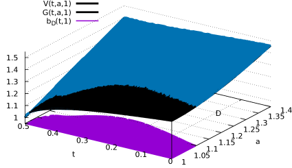
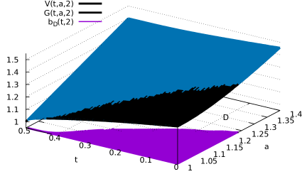
5 Numerical results
In this section we present numerical estimates
obtained from Theorems 2.1 2.2
b D ( t , j ) := inf { x ∈ [ 1 , ∞ ) : ( t , x , j ) ∈ D } , t ∈ [ 0 , T ] , j ∈ ℳ , formulae-sequence assign subscript 𝑏 𝐷 𝑡 𝑗 infimum conditional-set 𝑥 1 𝑡 𝑥 𝑗 𝐷 formulae-sequence 𝑡 0 𝑇 𝑗 ℳ b_{D}(t,j):=\inf\{x\in[1,\infty)\ :\ (t,x,j)\in D\},\quad t\in[0,T],\quad j\in{\cal M},
of the stopping set D 𝐷 D 1.7 ℳ = { 1 , 2 } ℳ 1 2 {\cal M}=\{1,2\}
In the absence of regime switching, the recursive algorithm
of Theorems 2.1 2.2 1 V ( t , a , j ) 𝑉 𝑡 𝑎 𝑗 V(t,a,j) G ( t , a , j ) 𝐺 𝑡 𝑎 𝑗 G(t,a,j) T = 1 𝑇 1 T=1 σ = 0.5 𝜎 0.5 \sigma=0.5 μ = 0.2 𝜇 0.2 \mu=0.2 n = 50 𝑛 50 n=50 δ n = T / n = 0.01 subscript 𝛿 𝑛 𝑇 𝑛 0.01 \delta_{n}=T/n=0.01
Figure 1 : Value functions computed from Theorems 2.1 2.2
Figure 1 D 𝐷 D 1.7 C = { ( t , a ) ∈ [ 0 , T ] × [ 1 , ∞ ) : V ( t , a ) < G ( t , a ) } 𝐶 conditional-set 𝑡 𝑎 0 𝑇 1 𝑉 𝑡 𝑎 𝐺 𝑡 𝑎 C=\big{\{}(t,a)\in[0,T]\times[1,\infty)\ :\ V(t,a)<G(t,a)\big{\}}
In Figure 2 1.3 b ( t ) 𝑏 𝑡 b(t)
Figure 2 : Boundary function computed from Theorems 2.1 2.2 vs (1.3
As shown in Figure 2 n 𝑛 n
( i i ) 𝑖 𝑖 (ii)
Figure 3 2.1 2.2 μ ( 1 ) = 0.2 𝜇 1 0.2 \mu(1)=0.2 μ ( 2 ) = − 0.2 𝜇 2 0.2 \mu(2)=-0.2 σ ( 1 ) = 0.5 𝜎 1 0.5 \sigma(1)=0.5 σ ( 2 ) = 0.3 𝜎 2 0.3 \sigma(2)=0.3 T = 0.5 𝑇 0.5 T=0.5 n = 100 𝑛 100 n=100 δ n = T / n = 0.05 subscript 𝛿 𝑛 𝑇 𝑛 0.05 \delta_{n}=T/n=0.05
𝐐 = [ − 2.5 2.5 2 − 2 ] . 𝐐 delimited-[] 2.5 2.5 2 2 \mathbf{Q}=\left[\begin{array}[]{cc}-2.5&2.5\\
2&-2\end{array}\right].
Figure 3 : Value functions under drifts of mixed signs.
Figure 3 D 𝐷 D
C = { ( t , a , j ) ∈ [ 0 , T ] × [ 1 , ∞ ) × ℳ : V ( t , a , j ) < G ( t , a , j ) } . 𝐶 conditional-set 𝑡 𝑎 𝑗 0 𝑇 1 ℳ 𝑉 𝑡 𝑎 𝑗 𝐺 𝑡 𝑎 𝑗 C=\big{\{}(t,a,j)\in[0,T]\times[1,\infty)\times{\cal M}\ :\ V(t,a,j)<G(t,a,j)\big{\}}.
The numerical instabilities observed are due to the necessity
to check the equality V ( t , a , j ) = G ( t , a , j ) 𝑉 𝑡 𝑎 𝑗 𝐺 𝑡 𝑎 𝑗 V(t,a,j)=G(t,a,j) V ( t , a , j ) 𝑉 𝑡 𝑎 𝑗 V(t,a,j) G ( t , a , j ) 𝐺 𝑡 𝑎 𝑗 G(t,a,j) t ↦ b D ( t , 1 ) maps-to 𝑡 subscript 𝑏 𝐷 𝑡 1 t\mapsto b_{D}(t,1) 1 1 1 t 𝑡 t 0 0 2 2 2 1 / q 1 , 1 = 0.4 1 subscript 𝑞 1 1
0.4 1/q_{1,1}=0.4 μ ( 2 ) = − 0.2 𝜇 2 0.2 \mu(2)=-0.2 t 𝑡 t 0.3 0.3 0.3 t ↦ b D ( t , 1 ) maps-to 𝑡 subscript 𝑏 𝐷 𝑡 1 t\mapsto b_{D}(t,1) 1 1 1 μ ( 1 ) = 0.2 𝜇 1 0.2 \mu(1)=0.2 1 / q 2 , 2 = 0.5 1 subscript 𝑞 2 2
0.5 1/q_{2,2}=0.5 T − t 𝑇 𝑡 T-t
Figure 4 : Boundary functions under drifts of mixed signs.
The boundary functions are plotted in Figure 4 2 2 2 t ↦ b D ( t , 2 ) maps-to 𝑡 subscript 𝑏 𝐷 𝑡 2 t\mapsto b_{D}(t,2) 0 0 T 𝑇 T 1 / q 2 , 2 = 0.5 1 subscript 𝑞 2 2
0.5 1/q_{2,2}=0.5 1 1 1 T − t 𝑇 𝑡 T-t
Until time 0.2 0.2 0.2 2 2 2 1 1 1 t 𝑡 t b ( t , 1 ) < Y ^ 0 , t / Y t = a < b D ( t , 2 ) 𝑏 𝑡 1 subscript ^ 𝑌 0 𝑡
subscript 𝑌 𝑡 𝑎 subscript 𝑏 𝐷 𝑡 2 b(t,1)<\hat{Y}_{0,t}/Y_{t}=a<b_{D}(t,2) 0.2 0.2 0.2 b ( t , 2 ) < Y ^ 0 , t / Y t = a < b D ( t , 1 ) 𝑏 𝑡 2 subscript ^ 𝑌 0 𝑡
subscript 𝑌 𝑡 𝑎 subscript 𝑏 𝐷 𝑡 1 b(t,2)<\hat{Y}_{0,t}/Y_{t}=a<b_{D}(t,1)