Candidate star clusters toward the inner Milky Way discovered on deep-stacked $K_{S}$-band images from the VVV Survey

Abstract

Context. The census of star clusters in the inner Milky Way is incomplete because of extinction and crowding.

Aims. We embarked on a program to expand the star cluster list in the direction of the inner Milky Way using deep stacks of K_S-band images from the VISTA Variables in Via L actea (VVV) Survey.

Methods. We applied an automated two-step procedure to the point-source catalog derived from the deep K_S images: first, we identified overdensities of stars, and then we selected only candidate clusters with probable member stars that match an isochrone with a certain age, distance, and extinction on the color-magnitude diagram.

Results. This pilot project only investigates the cluster population in part of one VVV tile, that is, b201. We identified nine cluster candidates and estimated their parameters. The new candidates are compact with a typical radius on the sky of $\sim$0.2–0.4 arcmin ($\sim$0.4–1.6 pc at their estimated distances). They are located at distances of $\sim$5–14 kpc from the Sun and are subject to moderate extinction of E($B$$-$$V$)=0.4–1.0 mag. They are sparse, probably evolved, with typical ages log($t$/1 yr)$\sim$9. Based on the locations of the objects inside the Milky Way, we conclude that one of these objects is probably associated with the disk or halo and the remaining objects are associated with the bulge or the halo.

Conclusions. The cluster candidates reported here push the VVV Survey cluster detection to the limit. These new objects demonstrate that the VVV survey has the potential to identify thousands of additional cluster candidates. The sub-arcsec angular resolution and the near-infrared wavelength regimen give it a critical advantage over other surveys.

1 Introduction

The star cluster searches in the general direction of the inner Milky Way are hampered by two obstacles: extinction and crowding. The clumpy structure of the dust makes it even harder to find clusters because both the often used visual inspection and the algorithms that identify density peaks can easily be deceived by holes in the dust or by sharp stellar density variation near the edges of dark clouds. It is not surprising that the first new generation cluster searches based on the Two Micron All Sky Survey (2MASS; Skrutskie et al. 2003) were limited to the vicinity of known objects that might be associated with clusters. For example, Dutra & Bica (2000) and Dutra & Bica (2001) looked for clusters around known HII regions or unidentified IRAS sources and in known star-forming regions, respectively.

Ivanov et al. (2002) and Borissova et al. (2003) attempted to find clusters blindly searching the 2MASS point source catalog for overdensities with automated tools and found some richer clusters. However, subsequent works (e.g., Mercer et al. 2005; Kronberger et al. 2006; Koposov et al. 2008; Camargo et al. 2015) continued to discover more objects, even from the same observational data sets, indicating that the cluster census still remained incomplete. Indeed, incompleteness was detected even in the most comprehensive clusters catalogs to date by other teams; Schmeja et al. (2014) identified a lack of old (t$\geq$1 Gyr) open clusters as close as the nearest 1 kpc from the Sun in the list of nearly $\sim$3800 clusters reported by Kharchenko et al. (2013).

New deeper surveys with better angular resolution became available in the meantime, in particular the VISTA Variables in Via L actea (VVV; Minniti et al. 2010; Saito et al. 2012). This motivated us to continue the search for new clusters. So far we have discovered in the VVV data in a total of 735 new star cluster candidates (Minniti et al. 2011; Moni Bidin et al. 2011; Borissova et al. 2011, 2014; Solin et al. 2014; Barbá et al. 2015), greatly improving the census of the star clusters in the Galaxy. Most of the newly identified objects are practically invisible in the optical.

Here we describe the results from a pilot project to identify cluster candidates aimed (i) as a proof of concept and (ii) to evaluate, at least approximately, the expected number of candidates yielded from a full VVV search. This project is a precursor for the LSST cluster searches, even though the LSST works in the optical, stacking multiple epochs as carried out in this work will generate deep images in the Milky Way. For simplicity, we ensured homogeneity by applying our algorithm to only one pawprint from one of the 348 VVV survey tiles, referred to in VVV as b201. There were no known clusters or cluster candidates in the surveyed area. The explored $\sim$1$\times$1.5 deg² area is centered at Galactic coordinates ($l$, $b$)$\sim$(350.5 deg, $-$9.5 deg) near the edge of the bulge. A tile near the outer edge of the VVV footprint was chosen for this test because it is less affected by extinction and crowding than the inner bulge and disk tiles.

2 Observational data

2.1 VVV Survey

The VVV is an European Southern Observatory (ESO) public survey of $\sim$562 deg² of the Milky Way (Minniti et al. 2010; Saito et al. 2012), split between the bulge and the southern disk. The survey was completed in 2016. The survey area was covered once, quasi-simultaneously in $ZYJHK_{S}$, and then 60-100 $K_{S}$ band epochs were obtained over $\sim$5–6 yr period for variability studies. The main goal of the VVV survey is to map our galaxy with RR Lyr and Cepheids in three dimensions (Dékány et al. 2015; Gran et al. 2016). But the enormous wealth of data generated by the VVV survey allows us to address a number of other questions, from proper motions (Beamín et al. 2013; Ivanov et al. 2013) to stellar clusters (Borissova et al. 2011, 2014; Barbá et al. 2015), variable stars (Navarro Molina et al. 2016) and even extragalactic sources in the zone of avoidance (Coldwell et al. 2014); this list is far from complete.

The survey was carried out with VISTA (Visual and Infrared Survey Telescope for Astronomy; Emerson et al. 2006), which is the ESO 4.1 m telescope located on Cerro Paranal. This telescope is equipped with VIRCAM (VISTA InfraRed CAMera; Dalton et al. 2006), which is a wide field near-infrared imager producing $\sim$1$\times$1.5 deg² tiles. The detectors are sensitive in the range from 0.9 $\mu$m to 2.4 $\mu$m. The data are processed with the VISTA Data Flow System (VDFS; Irwin et al. 2004; Emerson et al. 2004) pipeline at the Cambridge Astronomical Survey Unit (CASU). The data products are available either from the ESO Science Archive or from the specialized VISTA Science Archive. (VSA; Cross et al. 2012).

2.2 Deep-stacked K_S-band images

Stacking $K_{S}$ images taken at multiple epochs allows us to obtain deeper data. We chose to combine only the best seeing ($\leq$1.0 arcsec) epoch available until January 2015. In the case of tile b201, this constituted 35 images. Pawprints rather than tiles were stacked together for two reasons: first, this ensures that images from the same detectors were combined with the same detector characteristics (read noise, gain, etc.); second, the sources are usually located in the same region of each detector, making the final point spread function more stable than what it would have been if images with large offsets were combined.

The stacking was performed with the casutools v1.0.30 task imstack. The task makes use of the WCS; when source CSAU catalogs are provided as input for each epoch, as in our case, it does fit the plate coefficients in pixel space to refine the WCS in the input header relative to the reference image. Then, each image is resampled to the reference image, and the clipped average of each pixel scaled by the exposure time and weighted by the confidence value from each corresponding confidence map, is computed and recorded in the final image.

Next, we performed aperture photometry on the stacked image with the casutools task imcore with almost the same parameters as used by CASU to produce the single epoch source catalogs for VVV survey; we only adjusted the values of FWHM accordingly and set the radius of aperture for default photometric analysis (rcore parameter) to three pixels ($\sim$1 arcsec). The final aperture radius used to compute the photometry is three times rcore. The output consists of fits images, confidence maps, and source catalogs with identical structure and content as their single-epoch counterpart produced by CASU for the individual epochs.

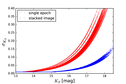
Figure 5: Photometric error as a function of $K_{S}$ magnitude for single epoch (red) and for a stacked image (blue). Only sources appearing in both catalogs are plotted.

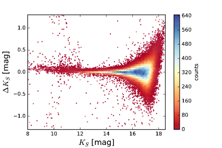
Figure 6: Photometric difference between the sources in the reference image and the stacked image. There is a small offset in the median value, but this offset is consistent with zero given the scatter in the data. This difference is probably related to the lower signal to noise in the reference image.

The improvement in number counts, depth, and photometric errors is shown in Figs. 1 and 5; the number of sources increased by a factor of $\sim$2.5 and the photometric error decreased considerably, particularly at the fainter end. We also cross-checked the photometry from the stacked image against the reference image (Fig. 6); the median difference is 0.035 mag with a median absolute deviation of 0.067 mag, so the difference is consistent with zero.

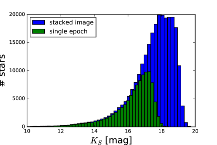
Figure 1: Number counts in single epoch (green) and in stacked image (blue) within 0.2 mag wide bins. The stacking increases the number counts by a factor of $\geq$2.5 and the depth by nearly 2 mag.

3 Cluster search and analysis

We applied the same search procedure as in Piatti et al. (2016), and we give here only a short summary of the steps. This procedure is based on identifying stellar surface density peaks after smoothing the surface density distribution with a kernel density estimator (KDE), which makes the density estimates independent from the bin size that is adopted in a “classical” two-dimensional histogram. We used the Python implementation available form the ASTROMIL library (VanderPlas et al. 2012); Gaussian and tophat KDEs were applied to the data with three different bandwidths of 0.23, 0.45, and 0.68 arcmin. In practical terms the kernels replace the individual points/stars, and then they are added gather to create continuous and smooth surface density map.

We run six different kernel overdensity searches on a sample of $\sim$266,000 stars from one pawprint from the stacked deep $K_{S}$-band image. Similar to Piatti et al. (2016) we adopted a cutoff density of 0.05 arcsec^-2, which is a factor of 1.25 higher than the typical background surface density of 0.04 arcsec^-2. This selection yielded 323 cluster candidates. We performed a visual inspection of the stacked $K_{S}$ image and three-color $JHK_{S}$ image made from single-epoch images of the VVV survey (Fig. 3), and we discard any candidates that could not be associated with obvious, well-pronounced stellar cluster-like concentrations. We estimated during the inspection the sizes and central positions of the candidates (Table 1). This left us with 36 candidates. Perhaps, some sparse clusters remained among the omitted object, but we prefer to err on the side of caution, instead of including questionable candidates in our sample.

The field star contamination was subtracted according the procedure of Piatti & Bica (2012). First we selected four comparison fields, each one with the same area as the cluster candidate, in the vicinity of the cluster. Then for each field star on the $K_{S}$ versus $Y$$-$$K_{S}$ color-magnitude diagram (CMD), we removed on the CMD of the cluster the nearest star to that field star. In the process we counted how many times each cluster star remained in the cleaned sample: if the cluster star remained all four times, the star was assigned 100% probability to be a member; if it remained three times, the membership probability was 75%, and so on. In the final analysis we only considered stars that have $\geq$50% likelihood of being members. An example of the results from the cleaning for the first object in our sample VVV CC 170 can be seen in Fig. 2. Diagrams for the rest of the cluster candidates are shown in Fig. 7. The plots for a given cluster contains CMDs of the cluster for different colors (top), a color-color diagram (bottom left), and a map that shows the location of the cluster with a black circle (bottom right). The cluster membership probability of individual stars is color coded; pink, light blue, and dark blue represent $\leq$25%, 50%, and $\geq$75$\%$, respectively.

Finally, we added to the CMDs theoretical solar-abundance isochrones for ages log($t$/1 yr) = 7.5, 8.0, 8.5, 9.0, 9.5, and 10.0 from Bressan et al. (2012). The isochrones were adjusted manually to reach the best fit to the data. The derived color excesses E($B$$-$$V$), distance moduli ($m$$-$$M$)₀, and ages log($t$/1 yr) are listed in Table 1. Conservatively, errors were tentatively adopted from the isochrones that bracket the best solution. Throughout this paper we use the extinction law of Nishiyama et al. (2006, 2008, 2009) and R_V=2.6 (Nataf et al. 2013). We discarded many candidates during this step, typically because the scatter around the best-fitting isochrones were large, indicating differential reddening; this is expected if instead of a cluster there is a hole in the dust. The remaining nine candidates were listed in our final sample (Table 1).

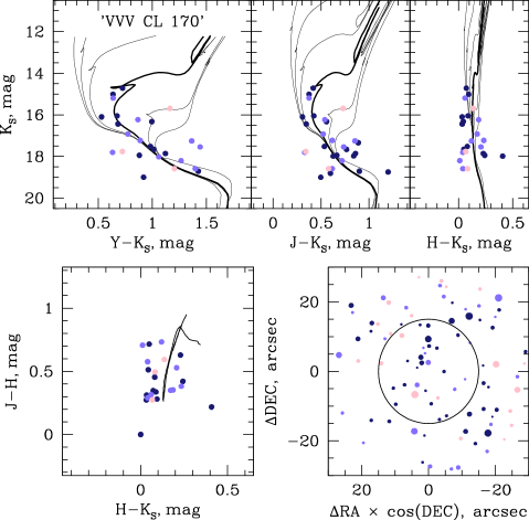
Figure 2: Top: Color-magnitude diagrams of the cluster VVV CC 170 (top). Solar abundance theoretical isochrones for ages log($t$/1 yr) = 7.5, 8.0, 8.5, 9.0, 9.5, and 10.0 from Bressan et al. (2012) are also shown. Bottom left: Color-color diagram. Only the log($t$/1 yr) = 9.0 isochrone is drawn for simplicity. Bottom right: A map of the cluster candidate. The black circle indicates the object size. On all panels the cluster candidate membership probabilities are color coded: dark blue implies $\geq$75$\%$, light blue is 50%, and pink indicates $\leq$25%, respectively. Similar plots for the other cluster candidates are shown in Fig. 7.

Table 1: Final cluster candidate sample with positions and derived parameters: angular and linear radii, color excess E($B$$-$$V$), distance modulus (m$-$M)₀, heliocentric distance D, distance below the Galactic plane plane $-$Z, galactocentric distance R_GC, and age. See Sec. 3 for details. The cluster IDs continue the nomenclature last used in Lima et al. (2014).

VVV	$\alpha$ $\delta$ (J2000)	Radius	E($B$$-$$V$)	(m$-$M)0	Distance D	$-$Z	RGC	Age
CC	deg	arcmin (pc)	mag	mag	kpc	kpc	kpc	log($t$/1 yr)
168	18:00:50.2 $-$42:11:31	0.4 (1.3)	1.0$\pm$0.5	15.2$\pm$0.5	11.0${}_{-5.2}^{+9.9}$	1.8${}_{-0.8}^{+1.6}$	3.8${}_{-0.8}^{+1.6}$	9.0$\pm$0.5
169	18:01:06.2 $-$42:04:15	0.25 (0.8)	0.7$\pm$0.5	15.3$\pm$0.5	11.5${}_{-5.4}^{+10.3}$	1.9${}_{-0.9}^{+1.7}$	4.3${}_{-0.8}^{+1.6}$	9.5$\pm$0.5
170	18:01:03.0 $-$42:03:09	0.25 (0.6)	1.0$\pm$0.5	14.5$\pm$0.5	7.9${}_{-3.8}^{+7.1}$	1.3${}_{-0.6}^{+1.2}$	1.9${}_{-1.1}^{+1.5}$	9.0$\pm$0.5
171	18:03:55.6 $-$42:20:07	0.25 (0.9)	1.0$\pm$0.5	15.5$\pm$0.3	12.6${}_{-5.8}^{+10.7}$	2.2${}_{-1.0}^{+1.8}$	5.4${}_{-0.7}^{+1.6}$	9.0$\pm$0.5
172	18:06:06.6 $-$42:09:46	0.3 (0.6)	0.5$\pm$0.5	14.2$\pm$0.5	6.9${}_{-3.3}^{+6.2}$	1.2${}_{-0.6}^{+1.1}$	2.0${}_{-0.7}^{+1.2}$	9.5$\pm$1.0
173	18:04:29.0 $-$41:41:33	0.3 (1.6)	0.6$\pm$0.5	13.5$\pm$0.5	5.0${}_{-2.7}^{+5.7}$	0.8${}_{-0.4}^{+1.0}$	3.3${}_{-0.0}^{+1.1}$	9.0$\pm$1.0
174	18:02:34.6 $-$41:31:08	0.4 (0.4)	0.9$\pm$0.5	15.7$\pm$1.0	13.8${}_{-6.5}^{+12.4}$	2.2${}_{-1.1}^{+2.0}$	6.4${}_{-0.5}^{+1.1}$	9.0$\pm$1.0
175	18:05:38.2 $-$41:43:58	0.3 (0.8)	0.4$\pm$0.5	14.7$\pm$0.5	8.7${}_{-4.1}^{+7.8}$	1.5${}_{-0.7}^{+1.3}$	2.1${}_{-1.0}^{+1.6}$	9.5$\pm$0.5
176	18:05:00.8 $-$41:22:49	0.2 (0.7)	0.9$\pm$0.3	15.5$\pm$0.5	12.6${}_{-4.4}^{+6.7}$	2.1${}_{-0.7}^{+1.1}$	5.3${}_{-0.5}^{+0.9}$	9.0$\pm$0.5

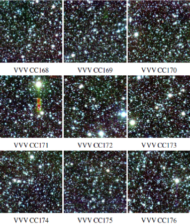
Figure 3: Three-color 3$\times$3 arcmin² finding charts ($Y$ - blue, $J$ - green, $K_{S}$ - red) of the candidate clusters. North is at the top left and east is to the top right.

4 Results and discussion

The final list of identified cluster candidates contains nine objects. Their locations on the sky are shown in Fig. 4 and there appears to be some clustering: VVV CC 169 and VVV CC 170 have projected on-sky separation of $\sim$2 arcmin, but these objects have different extinctions and distances (Table 1), so it is unlikely that they are physically connected. A physical connection between VVV CC 168 and VVV CC 169, separated by $\sim$9 arcmin and located at similar distances is more likely, but given the uncertainties, can only be tentative. The derived distances range between $\sim$5 kpc and $\sim$14 kpc, and our candidates are located $\sim$1–2 kpc below the Galactic plane. The candidate closest to us, VVV CC 169, may be associated with the Milky Way disk or halo. The remaining objects are probably part of the Milky Way bulge or halo, which comes as no surprise because their CMDs are consistent with an evolved stellar population with log($t$/1 yr)$\sim$9. The large uncertainties in the locations of the candidates and the lack of radial velocities prevent us from drawing firmer conclusions about which Milky Way component they belong to.

Figure 4: Location of our new cluster candidates in Galactic coordinates. The circle size is linearly proportional to the cluster radius but out of scale; the radius spans the range 0.2–0.4 arcmin. The objects are numbered according to Table 3. The x marks the center of tile b201.

We attempted to verify the stellar nature of the probable members of our final cluster candidate from the morphological class parameter derived by the CASU pipeline for the deep tiles. Unfortunately, this parameter is heavily affected by the crowding in the field; for the investigated pawprint, the total percentage of extended sources is unrealistically high, at nearly 40 %, and we can not attribute this to background galaxies. Instead, we compared the apparent $Y$$-$$K_{S}$ color of the members with those for some confirmed background galaxies in the VVV Survey from Coldwell et al. (2014) and found virtually no overlap: the galaxies span $Y$$-$$K_{S}$$\sim$1.5–2.2 mag, while the high-probability cluster members are bluer with $Y$$-$$K_{S}$$\leq$1.2–1.5 mag (Figs. 2 and 7).

Next, we investigated whether the cluster candidates could be holes in the Milky Way dust through which we can see the bulge population. The new objects are compact, and most of them have radii 15–18 arcsec, which is smaller than the spatial resolution of even the finest available reddening maps of the inner Milky Way, for example, 1$\arcmin$$\times$1$\arcmin$ for Gonzalez et al. (2013). This map reports for the fields of all our candidates E($J$$-$$K_{S}$)=0.0$\pm$0.1 mag, which in E($B$$-$$V$) implies 1$\sigma$ limits of $\sim$0.34 mag, which agrees at 2–3$\sigma$ level with all our CMD based estimates. We also inspected the WISE (Wide-field Infrared Survey Explorer; Wright et al. 2010) images and identified no obvious signature of circular dust emission around the objects.

The compact appearance of the new cluster candidates is probably the reason why they were not identified earlier Camargo et al. (e.g., 2015). In most cases the brightest member stars are in the range $K_{S}$$\sim$14–16 mag, placing them near the confusion limit of 2MASS in the inner Milky Way or even below that. The fainter member stars are beyond 2MASS detection, which might be the reason why these objects were not identified in the 2MASS searches either. In some cases the few brightest member stars can be seen on the DSS2 red and DSS2 IR images, but without the fainter stars it is difficult to realize that these may be overdensities associated with star clusters.

We treat the derived ages, extinctions, and distance moduli with care because an inspection of the CMDs in Figs. 2 and 7 shows that most color excesses and distances can easily vary by $\sim$0.5 mag, leading to a change of $\sim$0.5–1 in log($t$/1 yr).

None of the new candidates appear to be extremely young and the WISE images did not reveal any bright mid-infrared sources that may be associated with the new objects. The missing globulars that Ivanov et al. (2005) predicted might hide among these candidates. Unfortunately, the extinction and the distance make it difficult to characterize these objects spectroscopically Longmore et al. (e.g., 2011) and further investigations might have to rely on photometric techniques Ivanov & Borissova (e.g., 2002); Beletsky et al. (e.g., 2009).

Our candidates have smaller apparent sizes (listed in Table 1) than average radii $<$r$>$=0.6$\pm$0.4 arcmin of the infrared-selected star clusters and stellar groups listed by (Bica et al. 2003). However, the physical radii of the two samples our objects are similar: the peak of the distribution of linear diameters (figure 3 in Bica et al. 2003) corresponds to radii of 0.5–1 pc. A comparison with older objects, 141 globular clusters from the list of Harris (1996), indicates that the radii of most our candidates are bracketed between the average core radius $<$R_C$>$=0.5$\pm$0.6 pc and the average half-light radius $<$R_H$>$=1.3$\pm$0.8 pc of the globulars. Therefore, in terms of sizes the new candidates blend well with the samples of known cluster.

We conclude that the sub-arcsec angular resolution of the VVV survey in $K_{S}$ band was critical for uncovering these new cluster candidates. This survey fills in a niche between optical surveys that cannot penetrate the dust and the mid-infrared WISE survey, which can penetrate the dust, but the WISE suffers from poor angular resolution. Our result hints that the GLIMPSE survey (Galactic Legacy Infrared Mid-Plane Survey Extraordinaire; Benjamin et al. 2003) and its various extensions may be a fertile ground for future searches because they combine the dust penetration of the mid-infrared with the high angular resolution of VVV.

Our selection procedure relies on an automated repeatable density peaks selection, but it also includes manual verification steps, so it is not truly objective. This makes a cluster candidate catalog derived following this technique unsuitable for statistical studies of the clusters’ spatial distribution, age distribution, etc. If we simply scale up the number of candidates recovered from a single pawprint of a single VVV tile and keeping in mind that a pawprint only covers about 40 % of a tile, we can expect to recover thousands of candidates – preferentially low luminosity objects – from all 348 VVV tiles; the exact number is highly uncertain, given the limited number of the objects, but falls in line with the latest $\lambda$-CDM simulations (e.g., Schaye et al. 2015). This suggests that there should be thousands of faint Milky Way building blocks and the cluster candidates that we find might be the remnants of those.

5 Summary

We report results form an automated cluster selection based on deep stacked $K_{S}$-band images form the VVV survey. We identified more than 300 density peaks, but follow-up analysis indicated that the majority of them are likely false positives, so our final list contains only nine candidates. Most of these objects are probably evolved and many are associated with the bulge. The result from this search indicates that the entire VVV survey can yield thousands more Milky Way cluster candidates.

Appendix A Photometric properties of the deep-stacked VVV images

Appendix B Color-magnitude diagrams

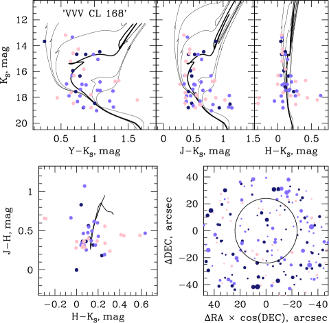
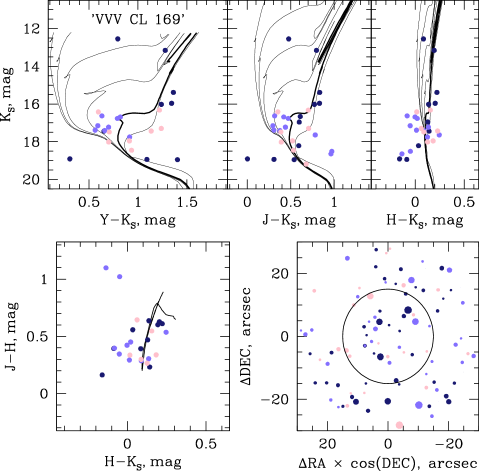
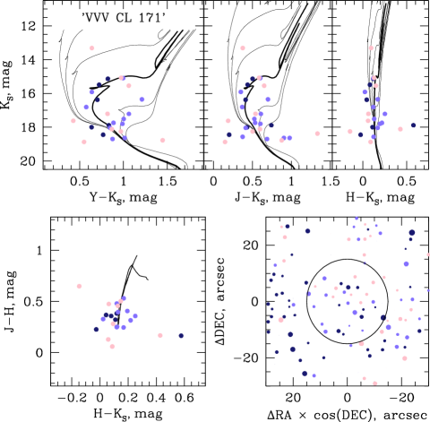
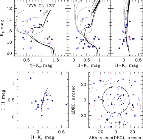
Figure 7: Color-magnitude diagrams of the cluster candidates VVV CC 168 (top left), VVV CC 169 (top right), VVV CC 171 (bottom left), and VVV CC 172 (bottom right). The subpanels and symbols are the same as in Fig. 2

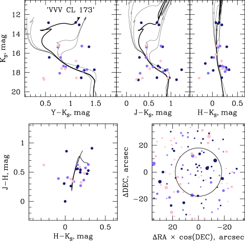
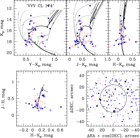
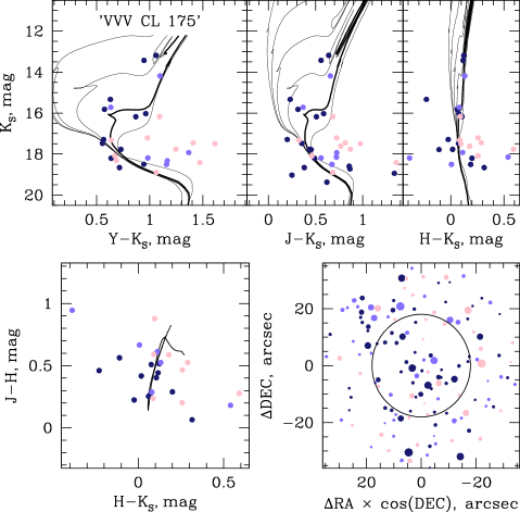
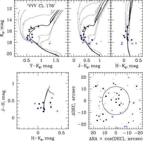
Figure 7: Continued. Color-magnitude diagrams of the cluster candidates VVV CC 173 (top left), VVV CC 174 (top right), VVV CC 175 (bottom left) and VVV CC 176 (bottom right). The sub-panels and symbols are the same as in Fig. 2