Analysis of a multi-mode plasmonic nano-laser with a inhomogeneous distribution of molecular emitters

Abstract

We extend Lamb’s reduced density matrix laser theory to analyze the inhomogeneous molecular couplings and the mode-correlation in a plasmonic nano-laser consisting of a gold sphere and many dye molecules interacting with a driving optical field and with the quantized plasmon modes. The molecular inhomogeneity is accounted for by simulating their random distribution around the sphere. Our analysis shows that in order to obtain lasing we must employ a large number of strongly driven molecules to compensate strong damping of the plasmon modes. The compact molecular arrangement, however, can lead to molecular energy-shifts and thus reduce the excitation of the plasmon modes and ultimately suggests a maximum limit for the plasmon excitation for any specific system.

I Introduction

The interaction between metals and light has been investigated for more than a century with Maxwell’s electromagnetic theory. One essential insight obtained is that the electromagnetic (EM) field is enhanced and localized around metal nano-particles (MNP) and on the interfaces between metallic films and dielectrics MPelton due to the excitation of surface plasmons involving collective oscillations of conductance electrons in the metal. The enhancement boosts the interaction between quantum emitters and the EM field MSTame ; RMMa-0 ; MPelton ; PBerini and thus leads to enhanced absorption NICade ; YZelinskyy , emission PAnger ; YZhang-4 and Raman scattering MFleischmann ; PJohansson . This can be utilized to improve the sensibility of spectroscopic instruments SYDing and the efficiency of LEDs XFGu ; NGao and solar cells HAAtwater ; LJWu .

The localization introduces EM modes with mode volumes that are not limited by the wavelength of free-space light YYin ; PBerini . These modes can be excited if externally pumped quantum emitters are placed near MNPs or metallic films. Under suitable conditions, the energy loss of those modes can be even compensated and the system can achieve lasing. This phenomenon known as SPASER, was proposed by Bergman and Stockman Bergman and verified firstly by Noginov, et. al. MANoginov with an experiment involving a gold nano-sphere and many dye molecules. Since then many experimental demonstrations have been reported with structures like semiconductor wires JHo ; RFOulton ; CYWu ; YJLu-1 ; YJLu ; YHou ; QZhang ; TPPHSi ; YHChou ; BTChou /squares RMMa ; RMMa-1 on metallic films, semiconductor pillars MTHill ; MPNezhad ; SHkwon ; JHLee ; MKha ; KDing /dots AMatsudira ; CYLu /wires CYLu-1 ; SWChang inside metallic cavities as well as dye molecules in periodically arranged MNP arrays JYSuh ; WZhou ; AYang ; AYang-1 ; AHSchokker .

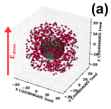
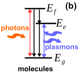
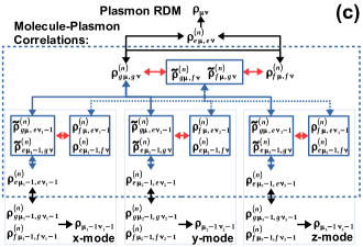
Figure 1: Panel (a) illustrates our system, composed of a gold nano-sphere ($10$ nm radius) surrounded by a layer ($12.5$ nm inner- and $22.5$ nm outer-radius) of $800$ randomly distributed dye molecules (blue dots) with randomly oriented transition dipole moments (the red arrows); the driving field is polarized along the $z$-axis. Panel (b) shows the effective three-level ($E_{g}$, $E_{e}$ and $E_{f}$) molecules interacting coherently with the driving field (the red arrow) and with the plasmons (the blue arrows) and experiencing dissipation (the black arrows). Panel (c) shows how the reduced density matrix elements of the plasmon modes $\rho_{\mu\nu}$ with $\mu\equiv\left\{\mu_{x}\mu_{y}\mu_{z}\right\}$ depend on the molecule-plasmon correlations $\rho_{a\mu,b\nu}^{\left(n\right)}$. The thin solid blue boxes indicate the correlations related to $x,y$, and $z$ modes (from left to right), and the colors of the arrows indicate the physical origin of the dependence, cf., panel (b). Approximate analytical expressions for the correlations are obtained to derive a closed set of equations for $\rho_{\mu\nu}$ (for more details see text).

In order to theoretically describe these systems, we have to determine the lasing modes and consider how the gain medium transfers energy to these modes. The modes can be analyzed by solving Maxwell’s equations analytically YHChou ; SWChang-1 or numerically JHo ; RFOulton ; CYWu ; YJLu-1 ; YJLu ; YHou ; QZhang ; TPPHSi ; YHChou ; BTChou ; MTHill ; MPNezhad ; SHkwon ; JHLee ; MKha ; KDing ; JYSuh ; WZhou ; AYang ; AYang-1 ; AHSchokker ; NLi . The energy transfer requires us to model the gain medium as a random spatial distribution of multi-level emitters. The multi-level model allows us to couple some levels with external driving fields or electron reservoirs to describe pumping mechanism and couple other levels with the lasing modes. It means that we have to deal with a complex theoretical problem involving many emitters, many levels and many modes. To reduce the complexity, semi-classical theories have been developed and utilized, for example, rate equations AMatsudira ; CYLu ; CYLu-1 and Maxwell-Bloch equations WZhou ; AYang ; AYang-1 . Because of the mean-field approximations involved, these theories, however, yield no statistical information about the the lasing modes and thus advanced full quantum laser theories are needed. Unfortunately, so far those quantum theories treat the emitters as identical two-level systems MRichter ; VMPar and are thus incapable of dealing with randomly distributed emitters.

Most existing theories can be viewed as effective descriptions, where the emitters are treated only in an average sense. They can reproduce main characteristics measured in experiments because the inhomogeneity of the emitters becomes irrelevant if huge amounts of them are involved. However, this may not be the case in the plasmonic nano-laser. Because of the strong inhomogeneous subwavelength distribution of the near-field in the nano-laser, the spatial distribution of emitters can significantly affect how they convert the pumping energy into the plasmon energy and even determine whether the systems can achieve lasing or not. By analyzing this influence, we can achieve more insights about the systems and more importantly understand how to improve the system performance by engineering the spatial distribution.

In this article, we provide a systematic analysis of the inhomogeneity of molecular emitters in a nano-laser of Fig. 1(a), which resembles the one studied in MANoginov . As the basis for our analysis, we will firstly describe our theoretical model in Sec. II. To account for multi-molecules and multi-modes, we have extended the density matrix laser theory of Lamb MSargent in our model. By following the procedure developed in YZhang ; YZhang-1 , we first establish a reduced density operator equation for the entire system and then derive a quantum master equation for the reduced density matrix (RDM) of the plasmon modes. Our extended theory allows us to analyze how the molecular distribution affects the plasmon statistics and the molecule-induced mode-correlations. This analysis is presented in Sec. III. In the end, we summarize our findings and present an outlook for future work.

II Theoretical Model

As indicated by Fig.1 (a), we consider a random arrangement of molecular emitters separated by more than $2.5$ nm from the surface of a gold nano-sphere of 10 nm radius. The separation guarantees that electron tunneling is suppressed KJSavage and the molecule-MNP coupling is dominated by Coulomb coupling. The molecules are assumed to be resonant with the dipole plasmons of the sphere. The higher multipole plasmons have minor influence on the system YZhang-3 and contribute only as an off-resonant reservoir to the excited-state decay rate of the molecules JGersten .

II.1 Reduced Density Operator Equation

For a nano-sphere, there are three degenerate dipole plasmon modes with transition dipole moments pointing along three orthogonal axes. Therefore, we can label them by $j=x,y,z$ or $j=1,2,3$. These modes can be described as quantum harmonic oscillators with Hamiltonian $H_{\mathrm{pl}}=\sum_{j}\hbar\omega_{j}C_{j}^{+}C_{j}$, where $C_{j}^{+}$ and $C_{j}$ are creation and annihilation operators and $\hbar\omega_{j}=\hbar\omega_{\mathrm{pl}}$ is their excitation energy Gweick . We describe the molecules as three-level systems with the internal energy level scheme and transitions shown in Fig.1(b). The molecular Hamiltonian reads $H_{{\rm e}}=\sum_{n=1}^{N_{{\rm e}}}\sum_{a_{n}}E_{na}\left|a_{n}\right\rangle\left\langle a_{n}\right|$ where ground states $\left|a_{n}=g_{n}\right\rangle$, first $\left|a_{n}=e_{n}\right\rangle$ and second $\left|a_{n}=f_{n}\right\rangle$ excited states have the energies $E_{ng}$,$E_{ne}$,$E_{nf}$, respectively ThreeLevels . We assume that the plasmon modes are resonant with the ground-to-first excited state transition, cf. the blue arrow in Fig.1(b), and introduces the coupling Hamiltonian $V_{{\rm pl-e}}=\hbar\sum_{n=1}^{N_{{\rm e}}}v_{ge}^{\left(jn\right)}\left(C_{j}^{+}\left|g_{n}\right\rangle\left\langle e_{n}\right|+{\rm h.c.}\right)$ in the rotating wave approximation. Here, the coefficient $\hbar v_{ge}^{\left(jn\right)}=\left[\mathbf{d}_{ge}^{\left(n\right)}\cdot\mathbf{d}_{j}-3\left(\mathbf{d}_{ge}^{\left(n\right)}\cdot\hat{\mathbf{x}}_{n}\right)\left(\mathbf{d}_{j}\cdot\hat{\mathbf{x}}_{n}\right)\right]/\left|\mathbf{X}_{n}\right|^{3}$ is determined by the transition dipole moment $\mathbf{d}_{ge}^{\left(n\right)}$ of the molecules, $\mathrm{\mathbf{d}}_{j}=d_{\mathrm{pl}}\mathrm{\mathbf{e}}_{j}$ of the plasmon modes as well as the distances $X_{n}$ and directional unit vectors $\hat{\mathbf{x}}_{n}$ connecting the $n^{\rm th}$ molecule and the sphere-center. We assume that a classical driving field is resonant with the ground-to-second excited state transition, cf. the red arrow in Fig.1(b), and introduces the coupling Hamiltonian $V_{{\rm e}}\left(t\right)=\hbar\sum_{n=1}^{N_{{\rm e}}}v_{gf}^{\left(n\right)}\left(e^{i\omega_{0}t}\left|g_{n}\right\rangle\left\langle f_{n}\right|+{\rm h.c.}\right)$ in the rotating wave approximation. Here, the coefficient $\hbar v_{gf}^{\left(n\right)}=\mathbf{d}_{gf}^{\left(n\right)}\cdot\mathbf{n}E_{0}$ is determined by another molecular transition dipole moment $\mathbf{d}_{gf}^{\left(n\right)}$ and the driving field is specified by a frequency $\omega_{0}$, a polarization vector $\mathbf{n}$ and an amplitude $E_{0}$ NFO . Here, we consider continuous optical excitation and thus $E_{0}$ is time-independent.

The density operator $\hat{\rho}$ for the quantized plasmon modes and the molecular emitters obeys the following quantum master equation

$$\frac{\partial}{\partial t}\hat{\rho}=-\frac{i}{\hbar}\left[H_{{\rm pl}}+H_{{\rm e}}+V_{{\rm pl-e}}+V_{{\rm e}}\left(t\right),\hat{\rho}\right]-\mathcal{D}\left[\hat{\rho}\right],$$ (1)

where the system dissipation is accounted for by the Lindblad terms:

$$\mathcal{D}\left[\hat{\rho}\right]=\left(1/2\right)\sum_{u}k_{u}\left(\left[\hat{L}_{u}^{+}\hat{L}_{u},\hat{\rho}\right]_{+}-2\hat{L}_{u}\hat{\rho}\hat{L}_{u}^{+}\right).$$ (2)

The damping of the plasmon modes is included by terms with $k_{u}=\gamma_{j}=\gamma_{\mathrm{pl}}$, $\hat{L}_{u}=C_{j}$ for each mode $j$. The decay processes of the molecules are included by terms with $k_{u}=k_{a\to b}^{\left(n\right)}$, $\hat{L}_{u}=\left|b_{n}\right\rangle\left\langle a_{n}\right|$ for $E_{na}>E_{nb}$ for each molecule, cf. the black arrows in Fig.1(b). For the sake of simplicity, we ignore pure molecular dephasing.

II.2 Plasmon Reduced Density Matrix Equation

The main goal of our analysis is to determine the plasmon state populations (probabilities) and correlations as quantified by the reduced density matrix (RDM) with elements $\rho_{\mu\nu}\equiv\text{tr}_{\text{S}}\left\{\hat{\rho}\left(t\right)\left|\nu\right\rangle\left\langle\mu\right|\right\}$, where $\text{tr}_{\text{S}}$ denotes the trace over the system and $\left|\mu\right\rangle\equiv\left|\mu_{x}\right\rangle\left|\mu_{y}\right\rangle\left|\mu_{z}\right\rangle$ and $\left|\nu\right\rangle\equiv\left|\nu_{x}\right\rangle\left|\nu_{y}\right\rangle\left|\nu_{z}\right\rangle$ denote product states of the plasmon occupation number Fock states. From Eq. (1), we observe that $\rho_{\mu\nu}$ depends on the molecule-plasmon correlations $\rho_{e\mu_{j}-1,g\nu}^{\left(n\right)}$, $\rho_{g\mu,e\nu_{j}-1}^{\left(n\right)}$ and $\rho_{e\mu,g\nu_{j}+1}^{\left(n\right)}$, $\rho_{g\mu_{j}+1,e\nu}^{\left(n\right)}$ with a general definition $\rho_{a\mu,b\nu}^{\left(n\right)}\equiv\text{tr}_{\text{S}}\left\{\hat{\rho}\left(t\right)\left|b_{n}\right\rangle\left\langle a_{n}\right|\times\left|\nu\right\rangle\left\langle\mu\right|\right\}$, cf. Appendix B.

The equations for the correlations also follow from Eq. (1). These equations result in dependence between the plasmon RDM and the correlations, shown in Fig. 1(c), which is caused by the couplings and the dissipation rates in the master equation (1). This dependence also indicates our procedure to solve those inter-dependent equations: Because both molecular and plasmonic dissipation rates contribute to the decay of the correlations, they must decay faster and thus may adiabatically MOScully follow the plasmon RDM elements which are only affected by the plasmon damping. Because of the molecular dissipation, the correlations represented within the blue dashed box of Fig. 1(c) depend on the correlations outside the box. Fortunately, they all can be expressed as functions of the plasmon RDM because of the symmetry hidden in the coupling Hamiltonians. Finally, we back substitute these expressions and obtain closed dynamic equations for the plasmon RDM, where the molecules contribute by several coefficients, cf. Eq.(87) in Appendix B.

The diagonal elements $P_{\mu}\equiv\rho_{\mu\mu}$ are the populations (the probabilities) of the plasmon number states $\left|\mu\right\rangle$ while the off-diagonal elements $\rho_{\mu\nu}$ ($\mu\neq\nu$) represent the coherence of the plasmons. Here, we focus on the populations by solving the equations for those diagonal elements:

$$\frac{\partial}{\partial t}P_{\mu}=-\sum_{j=1}^{3}\left[\left(\gamma_{j}\mu_{j}+\kappa{}_{\mu}^{\left(j\right)}\right)P_{\mu}-\sum_{k=1}^{3}\eta_{\mu}^{\left(jk\right)}P_{\mu_{k}-1}\right]$$

$$+\sum_{j=1}^{3}\left[\left(\gamma_{j}\left(\mu_{j}+1\right)+\kappa_{\mu_{j}+1}^{\left(j\right)}\right)P_{\mu_{j}+1}-\sum_{k=1}^{3}\eta_{\mu_{j}+1}^{\left(jk\right)}P_{\mu_{j}+1\mu_{k}-1}\right],$$ (3)

where the rates $\kappa_{\mu}^{\left(j\right)}\equiv-\sum_{n=1}^{N_{\mathrm{e}}}\alpha{}_{\mu\mu}^{\left(jn\right)}$ and $\eta_{\mu}^{\left(jk\right)}\equiv-\sum_{n=1}^{N_{\mathrm{e}}}\beta_{\mu\mu}^{\left(jkn\right)}$ include contributions from individual molecule $\alpha{}_{\mu\mu}^{\left(jn\right)}$ and $\beta_{\mu\mu}^{\left(jkn\right)}$ respectively, cf. Eqs. (88) and (89) in the Appendix B. Here, $\mu_{j}\pm 1$ for $j=x$ indicates $(\mu_{x}\pm 1,\mu_{y},\mu_{z})$ and $\mu_{j}+1\mu_{k}-1$ for $j=x$ and $k=y$ denotes $(\mu_{x}+1,\mu_{y}-1,\mu_{z})$. Since the former rates decrease the population of higher plasmon states but increase that of lower states, they can be interpreted as molecule-induced plasmon damping rates. Since the latter rates have the opposite effect on the population, they can be interpreted as molecule-induced plasmon pumping rates. The latter rates depend on two plasmon mode indices and thus account for correlation between different plasmon modes induced by the molecules. These rates can be considered as extended Einstein’s AB coefficients accounting for the multi-plasmon modes, the molecular pumping mechanism and the molecular inhomogeneity.

At steady-state the second line of Eq. (3) is recovered if we replace $\mu_{j}$ by $\mu_{j}+1$ on the right side of the first line, which suggests a recursion relation of the populations. We obtain such a relation by setting the first line to zero:

$$P_{\mu}=\frac{\sum_{k=1}^{3}\left(\sum_{j=1}^{3}\eta_{\mu}^{\left(jk\right)}\right)P_{\mu_{k}-1}}{\sum_{j=1}^{3}\left(\gamma_{j}\mu_{j}+\kappa{}_{\mu}^{\left(j\right)}\right)}.$$ (4)

Together with the normalization condition $\sum_{\mu}P_{\mu}=1$, the above relation can be utilized to easily calculate the populations according to the procedure outlined in Fig. 8 in Appendix B. Although $P_{\mu_{x}\mu_{y}\mu_{z}}$ contains all the information about the three dipole plasmons, it is more intuitive to consider physical quantities related to one or two dipole plasmon. We calculate them by tracing out one mode to get $P_{\mu_{x}\mu_{y}}=\sum_{\mu_{z}}P_{\mu_{x}\mu_{y}\mu_{z}}$, $P_{\mu_{y}\mu_{z}}=\sum_{\mu_{x}}P_{\mu_{x}\mu_{y}\mu_{z}}$ and $P_{\mu_{x}\mu_{z}}=\sum_{\mu_{y}}P_{\mu_{x}\mu_{y}\mu_{z}}$ (the joint population of two modes) or by tracing out two modes to get $P_{\mu_{x}}=\sum_{\mu_{y}\mu_{z}}P_{\mu_{x}\mu_{y}\mu_{z}}$, $P_{\mu_{y}}=\sum_{\mu_{x}\mu_{z}}P_{\mu_{x}\mu_{y}\mu_{z}}$ and $P_{\mu_{z}}=\sum_{\mu_{x}\mu_{y}}P_{\mu_{x}\mu_{y}\mu_{z}}$ (the reduced population of one mode). We can also quantify the strength of plasmon excitation with the so-called plasmon mean numbers: $N_{j}\equiv\sum_{\mu_{j}}\mu_{j}P_{\mu_{j}}$ and the plasmon statistics with the so-called (steady-state) second order correlation functions: $g_{j}^{\left(2\right)}(0)\equiv\sum_{\mu_{j}}\mu_{j}\left(\mu_{j}-1\right)P_{\mu_{j}}$. To analyze how the individual molecule contributes to the plasmon excitation, we can calculate the population of individual molecular states: $P_{g}^{\left(n\right)}\equiv\sum_{\mu}\rho_{g\mu,g\mu}^{\left(n\right)}$, $P_{f}^{\left(n\right)}\equiv\sum_{\mu}\rho_{f\mu,f\mu}^{\left(n\right)}$ and $P_{e}^{\left(n\right)}\equiv\sum_{\mu}\rho_{e\mu,e\mu}^{\left(n\right)}$, which are actually determined by $P_{\mu_{x}\mu_{y}\mu_{z}}$, cf. Eqs. (123), (124) and (125) in Appendix C.

III Results

The above theoretical model provides clues about how the molecular inhomogeneity may affect the system performance. The molecular inhomogeneity mainly originates from their positions and orientations of their transition dipole moments, which leads to that all the molecules interact with the three modes simultaneously but with random strengths. Since this situation is too complex, we shift its discussion to the end and first consider a special configuration where all the molecules are located along the equator of the gold sphere, cf. Fig.2 (a).

III.1 Configuration with Single Dipole Plasmon Mode

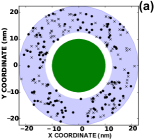
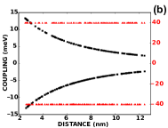
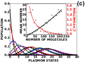
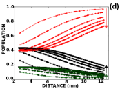
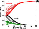
Figure 2: Configuration with single dipole plasmon mode. Panel (a): a gold nano-sphere (the green filled circle) with $240$ randomly distributed molecules in a layer ($r_{\mathrm{in}}=12.5$ inner- and $r_{\mathrm{out}}=22.5$ nm outer-radius); the black dots and crosses indicate the molecular transition dipole moment along the z-axis; the driving field is polarized along the positive $z$-axis. Panel (b): the coupling with the dipole plasmon (the black squares) and with the driving field (the red triangles) for molecules with different distances $d_{n}$ to the sphere-surface. Panel (c): plasmon state population $P_{\mu_{z}}$ for systems with increasing number of molecules $N_{\mathrm{e}}$ from $20$ to $220$ in a step of $20$ (from the left to right curve); the inset shows plasmon mean number $N_{z}$ (the black squares fitted with $-1.54+8.26\times 10^{-2}N_{\rm e}+1.54\times 10^{-4}N_{\rm e}^{2}$) and the $g_{z}^{\left(2\right)}(0)$-functions (the red octagons fitted with $0.74e^{-0.02N_{\mathrm{e}}}+0.98$) versus $N_{\mathrm{e}}$. Panel (d): population of molecular states $P_{a}^{\left(n\right)}$ versus $d_{n}$; $P_{g}^{\left(n\right)}$(the black squares and curves), $P_{e}^{\left(n\right)}$ (the red up-triangles and curves), $P_{f}^{\left(n\right)}$ (the green down-triangles and curves); the arrows on the right indicate the increase of $N_{\mathrm{e}}$. Panel (e-f): systems with different widths $W=r_{\mathrm{out}}-r_{\mathrm{in}}$ of the molecular layer (fixed molecular density); panel (e) shows $N_{z}$ (the black squares fitted with $-19.79e^{-0.72W}+18.49$) and $g_{z}^{2}\left(0\right)$-function (the red circles fitted with $0.50e^{-0.28W}+1.06$) ; panel (f) shows $P_{g}^{\left(n\right)}$, $P_{e}^{\left(n\right)}$ and $P_{f}^{\left(n\right)}$ versus $d_{n}$ with $W$ from $1$ nm to $100$ nm (the zoomed area in the inset); the arrows indicate the increase of $W$. Physical parameters are specified in Table 1 in Appendix A.

For the configuration in Fig. 2 (a), the molecule-plasmon coupling is reduced to $\hbar v_{ge}^{\left(jn\right)}=\delta_{j,z}\left(\pm d_{ge}^{(n)}d_{\rm pl}/X_{n}^{3}\right)$ with positive (negative) sign for the molecules oriented along the positive (negative) z-axis. Obviously, the dipole plasmon x- and y-mode are not involved and thus can be ignored in the following analysis. The coupling depends inversely on the cubic of the molecule-sphere center distance $X_{n}=a_{\rm MNP}+d_{n}$, cf. the black squares in Fig. 2 (b). Here, $a_{\rm MNP}$ is the radius of the sphere and $d_{n}$ the distance to the sphere-surface. In contrast, the driving field coupling $\hbar v_{gf}^{\left(n\right)}$ on the molecules depends only on the molecular orientations but not the positions, cf. the red triangles in Fig. 2 (b). If all the molecules have the same distance to the sphere-surface, they are equivalent and the resulting ideal system has been already analyzed in YZhang-1 . There, we focused on the pumping mechanism and found the optimal parameters of the system leading to the strongest plasmon excitation, cf. Table 1 in Appendix A. These parameters will be used as reference parameters for the following simulations.

To compensate the strong plasmon damping, the number of molecules coupled strongly with the plasmons is an essential parameter. It was demonstrated in the experiment XGMeng that the system properties like emission wavelength, intensity and pumping threshold strongly depend on the concentration (number) of the molecules. Here, we analyze this dependence from three aspects: density of molecules, spatial extension of molecular layer and molecular level shift.

As indicated by Fig.2 (b), the molecules close to the sphere couple strongly with the plasmons. Therefore, those molecules contribute more to the plasmon excitation than other molecules. By increasing the molecular density, we increase the number of molecules and thus the plasmon excitation. This is clearly reflected in Fig. 2 (c) by the increased populations $P_{\mu_{z}}$ of higher plasmon excited states and the increased plasmon mean number $N_{z}$ (the black dots and curve in the inset) with increasing number of molecules $N_{\mathrm{e}}$ from $10$ to $240$. For larger $N_{\mathrm{e}}$, $P_{\mu_{z}}$ resemble Poisson distributions indicating the formation of a coherent state and $N_{z}$ approaches $25$, which is much larger than unity and thus indicates that the system is lasing. This conclusion is further confirmed by the $g_{z}^{\left(2\right)}(0)$-function, cf. the red dots and red curve in the inset of Fig. 2 (c), which approaches unity for large $N_{\mathrm{e}}$, i.e. the Poisson limit. The fluctuation of the dots around the curves in the inset is caused by different molecular distribution in each simulation and may thus represent fluctuations encountered in experiments.

To understand why the increasing molecular density can increase the plasmon excitation, here, we analyze the state population for every molecule $P_{a}^{\left(n\right)}$, cf. Fig. 2(d). First, we notice that the molecule-plasmon coupling $V_{{\rm pl-e}}$ leads to reversible processes (spontaneous emission, stimulated emission and absorption of the plasmons) since it enters into our master equation as a coherent coupling, cf. Eq. (1). These processes tend to balance the population of the molecular excited states $P_{e}^{\left(n\right)}$ and ground states $P_{g}^{\left(n\right)}$. This leads to the reduced $P_{e}^{\left(n\right)}$, cf. the red curves and arrow, and the increased $P_{g}^{\left(n\right)}$, cf. the black curves and arrow, with increasing $N_{\mathrm{e}}$. In addition, because the reduced coupling with increasing distance $d_{n}$ (cf. in Fig. 2(b)) reduces the rate of the processes, the $P_{e}^{\left(n\right)}$ increase and $P_{g}^{\left(n\right)}$ decrease with increasing $d_{n}$. The population of the higher excited state $P_{f}^{\left(n\right)}$ is mainly determined by the strong decay rate from this state to the middle excited state and thus is always smaller than the other populations.

In the following, we consider the effect of varying the spatial extent (width $W$) of the molecular layer, cf. Fig. 2(e), which can also be studied in experiments like MANoginov ; XGMeng by precisely controlling the synthesis time of the molecular layer. In this case, the molecules are added far away from the sphere surface and will thus contribute less to the plasmon excitation because of the reduced molecule-plasmon coupling, cf. Fig. 2 (b). As a result, the plasmon mean number $N_{z}$ and the $g_{z}^{\left(2\right)}\left(0\right)$-function saturate for large $W$ as displayed by Fig. 2(e). In addition, we find that the data points are close to the fitted curve for small $W$ but fluctuate a lot for large $W$. This can be easily understood with the change of the molecular state population $P_{a}^{\left(n\right)}$, cf. Fig. 2(f). When $W$ increases from 1 nm to $30$ nm, $P_{g}^{\left(n\right)},P_{e}^{\left(n\right)},P_{f}^{\left(n\right)}$ change dramatically, cf. the zoomed inset, since all molecules contribute to the plasmon excitation. Therefore, $N_{z}$ increases and the molecular inhomogeneity has less influence on the plasmon excitation. However, when $W$ increases further, $P_{g}^{\left(n\right)},P_{e}^{\left(n\right)},P_{f}^{\left(n\right)}$ change less and now the molecules distributed in the region near to the sphere will significantly affect $N_{z}$.

The compact molecular arrangement around the sphere implies that the molecules may directly interact with each other through Coulomb coupling. If the molecular concentration is very high, electron transfer between molecules becomes possible. Although this process may be relevant here, it is however beyond the scope of our theory. For not too high concentration, the electron transfer can be ignored but direct energy exchange between excited molecular dipoles can lead to energy-shift (inhomogeneous broadening). In principle, such effect can be accurately described by directly incorporating the inter-molecular energy exchange coupling into the system Hamiltonian in the master equation (1). However, here, we follow an easier, phenomenological way to account for such effect by introducing random energy shift $\delta E^{\left(n\right)}$ to individual molecule with a Gaussian distribution HHaken , cf. Fig. 3 (a), $p\left(\delta E\right)=\left(1/\sqrt{2\pi}\sigma\right)\exp\left\{-\left(\delta E\right)^{2}/\left(2\sigma^{2}\right)\right\}$ (with standard deviation $\sigma$). It means that the transition energies are modified as $\hbar\omega_{eg}^{\left(n\right)}=\hbar\omega_{eg}+\delta E^{\left(n\right)}$ and $\hbar\omega_{fg}^{\left(n\right)}=\hbar\omega_{fg}+\delta E^{\left(n\right)}$, compared to the values in Table I in Appendix A.

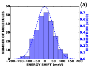
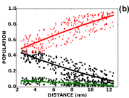
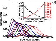
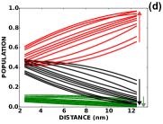
Figure 3: Effect of molecular energy-shift $\delta E^{\left(n\right)}$ for a system with $N_{\mathrm{e}}=250$ molecules. Panel (a): histogram of $\delta E^{\left(n\right)}$ as well as the Gaussian distribution with the deviation $\sigma=$50 meV. Panel (b): population of molecular states $P_{a}^{\left(n\right)}$ versus the molecular distance to the sphere-surface, $P_{g}^{\left(n\right)}$ (the black squares and curve), $P_{e}^{\left(n\right)}$ (the red up-triangles and curve), $P_{f}^{\left(n\right)}$ (the green down-triangles and curve); the random populations fitted by polynomial function. Panel (c): plasmon state population $P_{\mu_{z}}$ with increasing $\sigma$ from $0$ meV to $100$ meV in a step of $10$ meV (from the right to left curve); the inset: plasmon mean number $N_{z}$ (the black dots and curve) and $g_{z}^{\left(2\right)}\left(0\right)$-function (the red dots and curve). Panel (d): fitted populations of molecular states for increasing $\sigma$ indicated by the arrows. The strength of the driving field is $E_{0}=9\times 10^{7}$ $\mathrm{V/m}$. Physical parameters are specified in Table 1 in Appendix A.

The consequence of energy-shift is to perturb the perfect resonant condition for the molecular pumping and the molecule-plasmon energy transfer assumed previously. This is reflected by the irregular change of the state populations $P_{a}^{\left(n\right)}$ for the molecules at similar distances to the sphere surface, cf. the dots in Fig. 3 (b). However, since the majority of molecules has no or small energy shift as shown in Fig. 3 (a), the populations $P_{a}^{\left(n\right)}$ in Fig. 3 (b) still roughly follow the same trend observed in Fig. 2 (d), cf. the solid lines. The broadening of the transition energies is also reflected in the shift of the plasmon state population $P_{\mu_{z}}$ to lower states, a reduced plasmon mean number $N_{z}$ and an increased $g_{z}^{(2)}(0)$-function with increasing deviation $\sigma$ of the energy-shift from 0 meV to 100 meV, cf. Fig. 3 (c). These features can be understood by analyzing the contribution of individual molecule through their state populations $P_{a}^{\left(n\right)}$. As shown in Fig. 3 (d), the populations of the molecular middle excited states $P_{e}^{\left(n\right)}$ increase while those of the ground states $P_{g}^{\left(n\right)}$ decrease with increasing $\sigma$. These results reflect that the molecules are on average less affected by the plasmons and thus contribute less to the plasmon excitation. The features described above indicate that the lasing performance is strongly affected by the inhomogeneous molecular energy-shift. Finally, we point out that the standard deviation $\sigma$ characterizes energy-shifts due to intra-molecular interactions and should hence depends on the molecular concentration.

III.2 Configuration with Two and Three Dipole Plasmon Modes

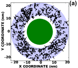
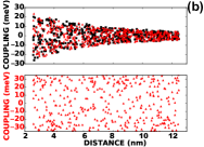
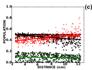
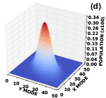
Figure 4: Configuration with two dipole plasmon modes. Panel (a): the configuration for $N_{\mathrm{e}}=500$ molecules is similar to Fig.2 (a) except that the molecular transition dipole moments orient randomly in the xy-plane and the driving field is along the positive $x$-axis. Panel (b): the couplings of molecules at different distances $d^{\left(n\right)}$ to the sphere-surface; the upper panel shows the coupling with the plasmon x-mode (the black squares), and with the plasmon y-mode (the red triangles); the lower panel shows the coupling with the driving field. Panel (c): the population of molecular states $P_{a}^{\left(n\right)}$ versus $d^{\left(n\right)}$ ; $P_{g}^{\left(n\right)}$ (the black squares), $P_{e}^{\left(n\right)}$ (the red upper triangles), $P_{f}^{\left(n\right)}$ (the green down triangles); the curves are exponentially fits to the average population as function of distance. Panel (d): joint population $P_{\mu_{x}\mu_{y}}$ of plasmon Fock states. Physical parameters are specified in Table 1 in Appendix A.

We now consider the more complex situation where the molecular transition dipole moments $\mathbf{d}_{ge}^{\left(n\right)}$ and $\mathbf{d}_{gf}^{\left(n\right)}$ orient randomly in the x-y plane, cf. Fig. 4(a). In this case, the molecules couple with the dipole plasmon $x-$ and $y-$mode simultaneously with random strength, cf. the upper panel of Fig. 4(b). In addition, the driving field coupling becomes also random as shown in the lower panel of Fig. 4(b) because it also depends on the orientations. This implies that the molecules at similar distance to the sphere-surface experience different couplings and this leads to the random population of molecular states $P_{a}^{\left(n\right)}$ as displayed in Fig. 4(c). However, because the maximum of the molecule-plasmon coupling decreases with increasing distance to the sphere-surface $d^{\left(n\right)}$, the distance-dependent averaged $P_{a}^{\left(n\right)}$ show a similar behavior as in Fig. 2(d). The co-existence of the x- and -y mode is directly illustrated by the joint plasmon state population $P_{\mu_{x}\mu_{y}}$ for a system with $N_{\mathrm{e}}=500$ molecules, cf. Fig. 4(d). Here, to better visualize $P_{\mu_{x}\mu_{y}}$, it is shown as a smooth surface. The population has a maximum around $\mu_{x}=25$ and $\mu_{y}=25$, which indicates that the both plasmon modes are excited to the same strength. In addition, we have also analyzed the plasmon state populations $P_{\mu_{x}},P_{\mu_{y}}$ , the plasmon mean numbers $N_{x},N_{y}$ and the $g_{x}^{\left(2\right)}\left(0\right)$- and $g_{y}^{\left(2\right)}\left(0\right)$-function for systems with increasing molecular density (number of molecules) in Fig. 6(a-c) and with increasing deviation $\sigma$ of molecular energy shift in Fig. 6(d-e) in Appendix A. Basically, they show similar features like those in Fig. 2(c) and Fig. 3 (c) respectively.

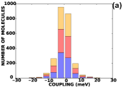
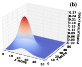
Figure 5: Configuration shown in Fig. 1(a) with three dipole plasmon modes. Panel (a): stacked histogram of the molecule-plasmon coupling; blue, red and orange bars are for x,y,z-mode respectively. Panel (b): the joint population $P_{\mu_{x}\mu_{y}}$ for a system with $800$ molecules. Physical parameters are specified the Table 1 in Appendix A.

Finally, let us turn to the realistic configuration of Fig. 1(a). In this case, the randomly distributed molecules in three dimensions couple with the three plasmon modes in a similar pattern, cf. Fig. 5 (a) (see also the coupling of individual molecule in Fig. 7 (a) in Appendix A). This implies that all the plasmon modes will be excited by the molecules in similar way and this is reflected by the joint populations $P_{\mu_{x}\mu_{y}}$, $P_{\mu_{y}\mu_{z}}$ and $P_{\mu_{x}\mu_{z}}$ with a peak around $\left(10,10\right)$ for a system with $N_{\rm e}=800$ molecules, cf. Fig. 5 (b) (see also Fig. 7 (b,c) in Appendix A). In addition, we also find the increased population $P_{\mu_{x}}$, $P_{\mu_{y}}$, $P_{\mu_{z}}$ of higher plasmon states, the increased plasmon mean number $N_{x},N_{y},N_{z}$ as well as the reduced $g_{x}^{\left(2\right)}\left(0\right),g_{y}^{\left(2\right)}\left(0\right),g_{z}^{\left(2\right)}\left(0\right)$-functions with increasing number of molecules $N_{\mathrm{e}}$ ( cf. Fig. 7(d,e,f) in Appendix A).

In order to achieve same plasmon excitation per mode, we must double (triple) the number of molecules in the case with two (three) modes compared to the single mode case. incidentally, our results show that the polarization of the driving field alone does not cause significant asymmetry between the excitation of the three plasmon modes.

IV Conclusions

In summary, we have developed a quantum laser theory based on reduced density matrix equation and applied it to a plasmonic nano-laser consisting of a gold nano-sphere and many dye molecules. Our study reveals that the molecular inhomogeneity and the multi-plasmon modes make strong molecular pumping necessary to compensate strong plasmon damping and to achieve lasing. By increasing the molecular density, the plasmon excitation increases, but molecular energy-shifts due to inter-molecular interaction may ultimately reduce the plasmon excitation.

In this article, we modeled the molecular emitters as three-level systems. However, the procedure illustrated can be readily applied to the emitters with arbitrary level structure, which will be necessary to study the influence of other intrinsic processes of the emitters on the laser performance. For example, by introducing more intermediate molecular vibrational levels, in principle, we can study how the intra-molecular vibrational energy redistribution and the temperature of the environment affect the system performance. This extended theory may be utilized to analyze the experiments AYang , where the varying excitation energy of lattice plasmons due to changing the surrounding material affects the dye molecules used by picking up the molecular energy levels resonant to the plasmons. This study will not only provide more insights about the interplay of the plasmons and the gain material but may also suggest how to optimize the system performance.

Appendix A System Parameters and Other Results

In Table 1, we list reference parameters for our simulations. We consider a gold nano-sphere with a radius of $10$ nm. The corresponding dipole plasmons have an excitation energy of $\hbar\omega_{\mathrm{pl}}=2.6$ eV, a damping rate $\hbar\gamma_{\mathrm{c}}=100$ meV and an optical transition dipole moment $d_{\mathrm{pl}}=2925$ D. The classical driving field has the photon energy $\hbar\omega_{0}=2.7$ eV and the amplitude $E_{0}=1.2\times 10^{8}$ V/m consistent with the values used in the experiments WZhou ; AYang ; AYang-1 ; XGMeng ; YJLu-1 ; YJLu ; RMMa ; CYWu ; QZhang ; KDing . The molecules have the transition energy $\hbar\omega_{eg}=2.6$ eV and the transition dipole moments $d_{gf}=16$ D and $d_{ge}=14.4$ D. The molecular transition energy $\hbar\omega_{fg}=2.7$ eV is off-resonant from the higher multipole plasmons YZhang-3 . The decay rate is $\hbar k_{f\to e}^{\left(n\right)}=100$ meV and we assume the other rates $k_{f\to g}^{\left(n\right)}$ and $k_{e\to g}^{\left(n\right)}$ can be ignored compared to the former decay rate.

In Fig. 6 and Fig. 7, we supplement the results presented in the main text with numerical results for system configurations with two and three dipole plasmons.

Table 1: Physical parameters (for explanation see text)

$\hbar\omega_{\mathrm{pl}}$	$2.6$ eV	$\hbar\omega_{eg}$	$2.6$ eV
$\hbar\gamma_{\mathrm{pl}}$	$100$ meV	$\hbar\omega_{fg}$	$2.7$ eV
$d_{\mathrm{pl}}$	$2925$ D	$d_{gf}$	$16$ D
$E_{0}$	$1.2\times 10^{8}$ V/m	$d_{ge}$	$14.4$ D
$\hbar\omega_{0}$	$2.7$ eV	$\hbar k_{f\to e}$	$100$ meV
		others	$0$ meV

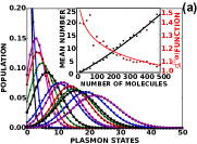
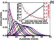
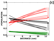
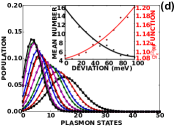
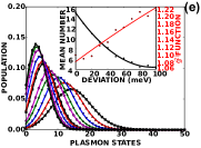
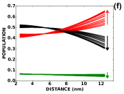
Figure 6: Supplemental results to Fig. 4. Configuration with two plasmon modes. Panel (a) shows the state populations $P_{\mu_{x}}$ of the plasmon x-mode with increasing number of molecules $N_{\mathrm{e}}$ from $20$ to $500$ in a step of $40$ (from the left to right curves); the inset shows the plasmon mean number $N_{x}$ and $g_{x}^{\left(2\right)}\left(0\right)$-function as functions of $N_{\mathrm{e}}$. Panel (b) shows $P_{\mu_{y}}$, $N_{y}$ and $g_{y}^{\left(2\right)}\left(0\right)$ as functions of $N_{\mathrm{e}}$. Panel (c) shows fitted populations $P_{a}^{\left(n\right)}$ of the molecular states as functions of the molecular distances $d^{\left(n\right)}$ to the sphere-surface (increasing values of $N_{\mathrm{e}}$ are indicated by the right arrows); $P_{g}^{\left(n\right)}$ (the black curves), $P_{e}^{\left(n\right)}$ (the red curves) and $P_{f}^{\left(n\right)}$ (the blue curves). Panel (d) shows $P_{\mu_{x}}$ ,$N_{x}$ and $g_{x}^{\left(2\right)}\left(0\right)$ for increasing deviation $\sigma$ of the molecular energy-shift, from $0$ meV to $100$ meV in a step of $10$ meV. Panel (e) shows $P_{\mu_{y}}$ ,$N_{y}$ and $g_{y}^{\left(2\right)}\left(0\right)$ versus $\sigma$. Panel (f) shows $P_{a}^{\left(n\right)}$ versus $d^{\left(n\right)}$ with the arrows indicating the increased $\sigma$. Physical parameters are specified in Table 1.

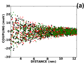
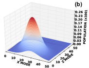
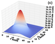
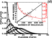
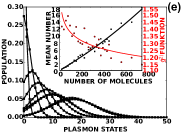
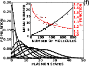
Figure 7: Supplemental results to Fig. 5. Configuration with three plasmon modes. In panel (a), blue squares, red upper-triangles and orange down-triangles show the coupling with the dipole plasmon x,y,z-mode for molecules with different distances to the sphere-surface. Panel (b,c) show the joint population $P_{\mu_{x}\mu_{z}}$ and $P_{\mu_{y}\mu_{z}}$ for a system with $800$ molecules. Panel (d) shows the reduced plasmon state population $P_{\mu_{x}}$ for increasing number of molecules $N_{\mathrm{e}}$; the inset shows the plasmon mean number $N_{x}$ and $g_{x}^{\left(2\right)}(0)$-function versus $N_{\mathrm{e}}$. Panel (e) is similar to panel (d) but shows $P_{\mu_{y}}$, $N_{y}$ and $g_{y}^{\left(2\right)}(0)$ of the $y$-mode. Panel (f) is similar to panel (d) but for $P_{\mu_{z}}$, $N_{z}$ and $g_{z}^{\left(2\right)}(0)$ of the $z$-mode. Physical parameters are specified in Table 1.

Appendix B Derivation of Plasmon Reduced Density Matrix Equation

In this section, we derive the master equation for the plasmon reduced density matrix (RDM) $\rho_{\mu\nu}$. From the definition of $\rho_{\mu\nu}$ and Eq. (1), we get the following equation:

$$\frac{\partial}{\partial t}\rho_{\mu\nu}=-\sum_{j=1}^{3}\left(i\omega_{j}\left(\mu_{j}-\nu_{j}\right)+\gamma_{j}\left[\left(\mu_{j}+\nu_{j}\right)/2\right]\right)\rho_{\mu\nu}$$

$$+\sum_{j=1}^{3}\gamma_{j}\sqrt{\left(\mu_{j}+1\right)\left(\nu_{j}+1\right)}\rho_{\mu_{j}+1\nu_{j}+1}$$

$$-i\sum_{n=1}^{N_{\mathrm{e}}}\sum_{j=1}^{3}v_{ge}^{\left(jn\right)}\Big{[}\sqrt{\mu_{j}}\rho_{e\mu_{j}-1,g\nu}^{\left(n\right)}-\sqrt{\nu_{j}}\rho_{g\mu,e\nu_{j}-1}^{\left(n\right)}$$

$$-\left(\sqrt{\nu_{j}+1}\rho_{e\mu,g\nu_{j}+1}^{\left(n\right)}-\sqrt{\mu_{j}+1}\rho_{g\mu_{j}+1,e\nu}^{\left(n\right)}\right)\Big{]}.$$ (5)

To simiplify notation, we consider $\rho_{\mu\nu}$ as a reference matrix element and denote the dependent matrix elements. For example, $\rho_{\mu_{j}+1\nu_{j}+1}$ differ from the reference element by increasing only the quantum number $\mu_{j}$ and $\nu_{j}$ by one. We see that $\rho_{\mu\nu}$ depends on the molecule-plasmon correlations: $\rho_{a\mu,b\nu}^{\left(n\right)}\equiv\text{tr}_{\text{S}}\left\{\hat{\rho}\left(t\right)\left|b_{n}\right\rangle\left\langle a_{n}\right|\times\left|\nu\right\rangle\left\langle\mu\right|\right\}$, more precisely, $\rho_{e\mu_{j}-1,g\nu}^{\left(n\right)}$, where the labels differ from the ones of $\rho_{e\mu,g\nu}^{\left(n\right)}$ only by subtracting $\mu_{j}$ by unity.

In the procedure to achieve an equation only for $\rho_{\mu\nu}$, the most crucial step is to analyze the equations for $\rho_{a\mu,b\nu}^{\left(n\right)}$ and express them as functions of $\rho_{\mu\nu}$. In the following, we present the equations for the population-like (coherence-like) correlations $\rho_{a\mu,a\nu}^{\left(n\right)}$ ($\rho_{a\mu,b\nu}^{\left(n\right)}$ with $a\neq b$). It turns out that these equations depend on the terms like $\gamma_{j}\sqrt{\left(\mu_{j}+1\right)\left(v_{j}+1\right)}\rho_{a\mu_{j}+1,b\nu_{j}+1}^{\left(n\right)}$ due to the damping from higher plasmon states. To avoid this dependence, we carry out the following replacement in all the equations for $\rho_{a\mu,b\nu}^{\left(n\right)}$:

$$-\sum_{j}\Big{(}\left[i\omega_{\mu\nu}-\gamma_{j}\left(\mu_{j}+\nu_{j}\right)/2\right]\rho_{a\mu,b\nu}^{\left(n\right)}$$

$$+\gamma_{j}\sqrt{\left(\mu_{j}+1\right)\left(\nu_{j}+1\right)}\rho_{a\mu_{j}+1,b\nu_{j}+1}^{\left(n\right)}\Big{)}\to-i\tilde{\omega}_{\mu\nu}\rho_{a\mu,b\nu}^{\left(n\right)}.$$ (6)

Here, we have introduced the complex transition frequency:

$$\tilde{\omega}_{\mu\nu}=\sum_{j}\Big{(}\omega_{j}\left(\mu_{j}-\nu_{j}\right)-i\gamma_{j}\left[\left(\mu_{j}+\nu_{j}\right)/2-\sqrt{\mu_{j}\nu_{j}}\right]\Big{)}.$$ (7)

Now, we start with the equations for the population-like correlation $\rho_{a\mu,a\nu}^{\left(n\right)}$ (density matrix elements with same molecular states):

$$\frac{\partial}{\partial t}\rho_{g\mu,g\nu}^{\left(n\right)}=-i\tilde{\omega}_{\mu\nu}\rho_{g\mu,g\nu}^{\left(n\right)}-\left(k_{g\to f}^{\left(n\right)}+k_{g\to e}^{\left(n\right)}\right)\rho_{g\mu,g\nu}^{\left(n\right)}$$

$$+k_{f\to g}^{\left(n\right)}\rho_{f\mu,f\nu}^{\left(n\right)}+k_{e\to g}^{\left(n\right)}\rho_{e\mu,e\nu}^{\left(n\right)}-iv_{gf}^{\left(n\right)}\left(\tilde{\rho}_{f\mu,g\nu}^{\left(n\right)}-\tilde{\rho}_{g\mu,f\nu}^{\left(n\right)}\right)$$

$$+i\sum_{j=1}^{3}v_{ge}^{\left(jn\right)}\left(\sqrt{\nu_{j}}\rho_{g\mu,e\nu_{j}-1}^{\left(n\right)}-\sqrt{\mu_{j}}\rho_{e\mu_{j}-1,g\nu}^{\left(n\right)}\right),$$ (8)

$$\frac{\partial}{\partial t}\rho_{f\mu,f\nu}^{\left(n\right)}=-i\tilde{\omega}_{\mu\nu}\rho_{f\mu,f\nu}^{\left(n\right)}-\left(k_{f\to g}^{\left(n\right)}+k_{f\to e}^{\left(n\right)}\right)\rho_{f\mu,f\nu}^{\left(n\right)}$$

$$+k_{g\to f}^{\left(n\right)}\rho_{g\mu,g\nu}^{\left(n\right)}+k_{e\to f}^{\left(n\right)}\rho_{e\mu,e\nu}^{\left(n\right)}+iv_{gf}^{\left(n\right)}\left(\tilde{\rho}_{f\mu,g\nu}^{\left(n\right)}-\tilde{\rho}_{g\mu,f\nu}^{\left(n\right)}\right),$$ (9)

$$\frac{\partial}{\partial t}\rho_{e\mu_{j}-1,e\nu_{j}-1}^{\left(n\right)}=-i\tilde{\omega}_{\mu_{j}-1\nu_{j}-1}\rho_{e\mu_{j}-1,e\nu_{j}-1}^{\left(n\right)}+k_{g\to e}^{\left(n\right)}\rho_{g\mu_{j}-1,g\nu_{j}-1}^{\left(n\right)}$$

$$-\left(k_{e\to g}^{\left(n\right)}+k_{e\to f}^{\left(n\right)}\right)\rho_{e\mu_{j}-1,e\nu_{j}-1}^{\left(n\right)}+k_{f\to e}^{\left(n\right)}\rho_{f\mu_{j}-1,f\nu_{j}-1}^{\left(n\right)}$$

$$+iv_{ge}^{\left(jn\right)}\left(\sqrt{\nu_{j}}\rho_{e\mu_{j}-1,g\nu}^{\left(n\right)}-\sqrt{\mu_{j}}\rho_{g\mu,e\nu_{j}-1}^{\left(n\right)}\right).$$ (10)

Then, we present the equations for the coherence-like correlations $\rho_{a\mu,b\nu}^{\left(n\right)}$ (density matrix elements with different molecular states) appearing in Eqs. (8), (9) and (10):

$$\frac{\partial}{\partial t}\tilde{\rho}_{g\mu,f\nu}^{\left(n\right)}=-i\left(\tilde{\omega}_{gf}^{\left(n\right)}+\tilde{\omega}_{\mu\nu}\right)\tilde{\rho}_{g\mu,f\nu}^{\left(n\right)}$$

$$-i\sum_{j=1}^{3}v_{ge}^{\left(jn\right)}\sqrt{\mu_{j}}\tilde{\rho}_{e\mu_{j}-1,f\nu}^{\left(n\right)}-iv_{gf}^{\left(n\right)}\left(\rho_{f\mu,f\nu}^{\left(n\right)}-\rho_{g\mu,g\nu}^{\left(n\right)}\right),$$ (11)

$$\frac{\partial}{\partial t}\tilde{\rho}_{f\mu,g\nu}^{\left(n\right)}=i\left(\tilde{\omega}_{gf}^{\left(n\right)*}-\tilde{\omega}_{\mu\nu}\right)\tilde{\rho}_{f\mu,g\nu}^{\left(n\right)}$$

$$+i\sum_{j=1}^{3}v_{ge}^{\left(jn\right)}\sqrt{v_{j}}\tilde{\rho}_{f\mu,e\nu_{j}-1}^{\left(n\right)}+iv_{gf}^{\left(n\right)}\left(\rho_{f\mu,f\nu}^{\left(n\right)}-\rho_{g\mu,g\nu}^{\left(n\right)}\right),$$ (12)

$$\frac{\partial}{\partial t}\rho_{g\mu,e\nu_{j}-1}^{\left(n\right)}=i\left(\tilde{\omega}_{eg}^{\left(n\right)*}-\tilde{\omega}_{\mu\nu_{j}-1}\right)\rho_{g\mu,e\nu_{j}-1}^{\left(n\right)}-iv_{gf}^{\left(n\right)}\rho_{f\mu,e\nu_{j}-1}^{\left(n\right)}$$

$$+iv_{ge}^{\left(jn\right)}\left(\sqrt{\nu_{j}}\rho_{g\mu,g\nu}-\sqrt{\mu_{j}}\rho_{e\mu_{j}-1,e\nu_{j}-1}^{\left(n\right)}\right),$$ (13)

$$\frac{\partial}{\partial t}\rho_{e\mu_{j}-1,g\nu}^{\left(n\right)}=-i\left(\tilde{\omega}_{eg}^{\left(n\right)}+\tilde{\omega}_{\mu_{j}-1\nu}\right)\rho_{e\mu_{j}-1,g\nu}^{\left(n\right)}+iv_{gf}^{\left(n\right)}\rho_{e\mu_{j}-1,f\nu}^{\left(n\right)}$$

$$+iv_{ge}^{\left(jn\right)}\left(\sqrt{\nu_{j}}\rho_{e\mu_{j}-1,e\nu_{j}-1}^{\left(n\right)}-\sqrt{\mu_{j}}\rho_{g\mu,g\nu}\right),$$ (14)

$$\frac{\partial}{\partial t}\tilde{\rho}_{e\mu_{j}-1,f\nu}^{\left(n\right)}=-i\left(\tilde{\omega}_{ef}^{\left(n\right)}+\tilde{\omega}_{\mu_{j}-1\nu}\right)\tilde{\rho}_{e\mu_{j}-1,f\nu}^{\left(n\right)}$$

$$+iv_{gf}^{\left(n\right)}\rho_{e\mu_{j}-1,g\nu}^{\left(n\right)}-iv_{ge}^{\left(jn\right)}\sqrt{\mu_{j}}\rho_{g\mu,f\nu}^{\left(n\right)},$$ (15)

$$\frac{\partial}{\partial t}\rho_{f\mu,e\nu_{j}-1}^{\left(n\right)}=i\left(\tilde{\omega}_{ef}^{\left(n\right)*}-\tilde{\omega}_{\mu\nu_{j}-1}\right)\rho_{f\mu,e\nu_{j}-1}^{\left(n\right)}$$

$$-iv_{gf}^{\left(n\right)}\tilde{\rho}_{g\mu,e\nu_{j}-1}^{\left(n\right)}+iv_{ge}^{\left(jn\right)}\sqrt{\nu_{j}}\tilde{\rho}_{f\mu,g\nu}^{\left(n\right)}.$$ (16)

In the above equations, we have introduced the complex transition frequencies: $\tilde{\omega}_{eg}^{\left(n\right)}=\omega_{eg}^{\left(n\right)}-i\gamma_{eg}^{\left(n\right)}$ with the dephasing rate $\gamma_{eg}^{\left(n\right)}=\left(k_{e\to g}^{\left(n\right)}+k_{e\to f}^{\left(n\right)}+k_{g\to e}^{\left(n\right)}+k_{g\to f}^{\left(n\right)}\right)/2$ and $\tilde{\omega}_{ef}^{\left(n\right)}=\omega_{ef}^{\left(n\right)}+\omega_{0}-i\gamma_{ef}^{\left(n\right)}$ with $\gamma_{ef}^{\left(n\right)}=\left(k_{e\to g}^{\left(n\right)}+k_{e\to f}^{\left(n\right)}+k_{f\to g}^{\left(n\right)}+k_{f\to e}^{\left(n\right)}\right)/2$ as well as $\tilde{\omega}_{gf}^{\left(n\right)}=\omega_{gf}^{\left(n\right)}+\omega_{0}-i\gamma_{gf}^{\left(n\right)}$ with $\gamma_{gf}^{\left(n\right)}\equiv\left(k_{f\to e}^{\left(n\right)}+k_{f\to g}^{\left(n\right)}+k_{g\to e}^{\left(n\right)}+k_{g\to f}^{\left(n\right)}\right)/2$. In addition, we would like to point out that the pure dephasing rate of the emitters can be readily included into these dephasing rates. Because of the coupling with the driving field, we have introduced the following slowly varying correlations $\tilde{\rho}_{e\mu_{j}-1,g\nu}^{\left(n\right)}\equiv e^{-i\omega_{0}t}\rho_{e\mu_{j}-1,g\nu}^{\left(n\right)}$, $\tilde{\rho}_{g\mu,e\nu_{j}-1}^{\left(n\right)}\equiv e^{i\omega_{0}t}\rho_{g\mu,e\nu_{j}-1}^{\left(n\right)}$, $\tilde{\rho}_{f\mu,g\nu}^{\left(n\right)}\equiv e^{i\omega_{0}t}\rho_{f\mu,g\nu}^{\left(n\right)}$ and $\tilde{\rho}_{g\mu,f\nu}^{\left(n\right)}\equiv e^{-i\omega_{0}t}\rho_{g\mu,f\nu}^{\left(n\right)}$.

To proceed, we consider the steady-state equations for the coherence-like correlations (density matrix elements with different molecular states). From Eqs. (13) , (14), (15) and (16) we have

$$\left(\tilde{\omega}_{eg}^{\left(n\right)*}-\tilde{\omega}_{\mu\nu_{j}-1}\right)\rho_{g\mu,e\nu_{j}-1}^{\left(n\right)}=v_{gf}^{\left(n\right)}\rho_{f\mu,e\nu_{j}-1}^{\left(n\right)}$$

$$-v_{ge}^{\left(jn\right)}\left(\sqrt{\nu_{j}}\rho_{g\mu,g\nu}-\sqrt{\mu_{j}}\rho_{e\mu_{j}-1,e\nu_{j}-1}^{\left(n\right)}\right),$$ (17)

$$\left(\tilde{\omega}_{eg}^{\left(n\right)}+\tilde{\omega}_{\mu_{j}-1\nu}\right)\rho_{e\mu_{j}-1,g\nu}^{\left(n\right)}=v_{gf}^{\left(n\right)}\rho_{e\mu_{j}-1,f\nu}^{\left(n\right)}$$

$$-v_{ge}^{\left(jn\right)}\left(\sqrt{\mu_{j}}\rho_{g\mu,g\nu}-\sqrt{\nu_{j}}\rho_{e\mu_{j}-1,e\nu_{j}-1}^{\left(n\right)}\right),$$ (18)

$$\left(\tilde{\omega}_{ef}^{\left(n\right)}+\tilde{\omega}_{\mu_{j}-1\nu}\right)\tilde{\rho}_{e\mu_{j}-1,f\nu}^{\left(n\right)}=v_{gf}^{\left(n\right)}\rho_{e\mu_{j}-1,g\nu}^{\left(n\right)}-v_{ge}^{\left(jn\right)}\sqrt{\mu_{j}}\rho_{g\mu,f\nu}^{\left(n\right)},$$ (19)

$$\left(\tilde{\omega}_{ef}^{\left(n\right)*}-\tilde{\omega}_{\mu\nu_{j}-1}\right)\rho_{f\mu,e\nu_{j}-1}^{\left(n\right)}=v_{gf}^{\left(n\right)}\tilde{\rho}_{g\mu,e\nu_{j}-1}^{\left(n\right)}-v_{ge}^{\left(jn\right)}\sqrt{\nu_{j}}\tilde{\rho}_{f\mu,g\nu}^{\left(n\right)}.$$ (20)

In order to reduce the dependence, we insert Eqs. (17) and (18) to Eqs. (19) and (20) to express $\tilde{\rho}_{e\mu_{j}-1,f\nu}^{\left(n\right)}$ and $\rho_{f\mu,e\nu_{j}-1}^{\left(n\right)}$ as functions of $\rho_{g\mu,f\nu}^{\left(n\right)}$, $\rho_{e\mu_{j}-1,e\nu_{j}-1}^{\left(n\right)}$ and $\rho_{g\mu,g\nu}$:

$$\tilde{\rho}_{e\mu_{j}-1,f\nu}^{\left(n\right)}=-\Xi_{\mu\nu}^{\left(jn\right)}v_{ge}^{\left(jn\right)}\sqrt{\mu_{j}}\rho_{g\mu,f\nu}^{\left(n\right)}$$

$$+v_{gf}^{\left(n\right)}\Sigma_{\mu\nu}^{\left(jn\right)}\Xi_{\mu\nu}^{\left(jn\right)}\left(\sqrt{\nu_{j}}\rho_{e\mu_{j}-1,e\nu_{j}-1}^{\left(n\right)}-\sqrt{\mu_{j}}\rho_{g\mu,g\nu}\right),$$ (21)

$$\rho_{f\mu,e\nu_{j}-1}^{\left(n\right)}=-\tilde{\Xi}_{\mu\nu}^{\left(jn\right)}v_{ge}^{\left(jn\right)}\sqrt{\nu_{j}}\tilde{\rho}_{f\mu,g\nu}^{\left(n\right)}$$

$$+v_{gf}^{\left(n\right)}\tilde{\Sigma}_{\mu\nu}^{\left(jn\right)}\tilde{\Xi}_{\mu\nu}^{\left(jn\right)}\left(\sqrt{\mu_{j}}\rho_{e\mu_{j}-1,e\nu_{j}-1}^{\left(n\right)}-\sqrt{\nu_{j}}\rho_{g\mu,g\nu}\right),$$ (22)

with the abbreviations:

$$1/\Xi_{\mu\nu}^{\left(jn\right)} =\tilde{\omega}_{ef}^{\left(n\right)}+\tilde{\omega}_{\mu_{j}-1\nu}-v_{gf}^{\left(n\right)2}/\left(\tilde{\omega}_{eg}^{\left(n\right)}+\tilde{\omega}_{\mu_{j}-1\nu}\right),$$ (23)

$$1/\tilde{\Xi}_{\mu\nu}^{\left(jn\right)} =\tilde{\omega}_{ef}^{\left(n\right)*}-\tilde{\omega}_{\mu\nu_{j}-1}-v_{gf}^{\left(n\right)2}/\left(\tilde{\omega}_{eg}^{\left(n\right)*}-\tilde{\omega}_{\mu\nu_{j}-1}\right),$$ (24)

$$\Sigma_{\mu\nu}^{\left(jn\right)}=v_{ge}^{\left(jn\right)}/\left(\tilde{\omega}_{eg}^{\left(n\right)}+\tilde{\omega}_{\mu_{j}-1\nu}\right),$$ (25)

$$\tilde{\Sigma}_{\mu\nu}^{\left(jn\right)}=v_{ge}^{\left(jn\right)}/\left(\tilde{\omega}_{eg}^{\left(n\right)*}-\tilde{\omega}_{\mu\nu_{j}-1}\right).$$ (26)

Then, we consider the steady-state version of Eqs. (11) and (12):

$$\left(\tilde{\omega}_{gf}^{\left(n\right)}+\tilde{\omega}_{\mu\nu}\right)\tilde{\rho}_{g\mu,f\nu}^{\left(n\right)}=v_{gf}^{\left(n\right)}\left(\rho_{g\mu,g\nu}^{\left(n\right)}-\rho_{f\mu,f\nu}^{\left(n\right)}\right)$$

$$-\sum_{j=1}^{3}v_{ge}^{\left(jn\right)}\sqrt{\mu_{j}}\tilde{\rho}_{e\mu_{j}-1,f\nu}^{\left(n\right)},$$ (27)

$$\left(\tilde{\omega}_{gf}^{\left(n\right)*}-\tilde{\omega}_{\mu\nu}\right)\tilde{\rho}_{f\mu,g\nu}^{\left(n\right)}=v_{gf}^{\left(n\right)}\left(\rho_{g\mu,g\nu}^{\left(n\right)}-\rho_{f\mu,f\nu}^{\left(n\right)}\right)$$

$$-\sum_{j=1}^{3}v_{ge}^{\left(jn\right)}\sqrt{v_{j}}\tilde{\rho}_{f\mu,e\nu_{j}-1}^{\left(n\right)}.$$ (28)

Finally, we insert Eqs.(21) and (22) to Eqs.(27) and (28) to express $\tilde{\rho}_{g\mu,f\nu}^{\left(n\right)}$ and $\tilde{\rho}_{f\mu,g\nu}^{\left(n\right)}$ as functions of the population-like correlations:

$$\tilde{\rho}_{g\mu,f\nu}^{\left(n\right)}=v_{gf}^{\left(n\right)}\Phi_{\mu\nu}^{\left(n\right)}\left(\rho_{g\mu,g\nu}^{\left(n\right)}-\rho_{f\mu,f\nu}^{\left(n\right)}\right)$$

$$-v_{gf}^{\left(n\right)}\Phi_{\mu\nu}^{\left(n\right)}\sum_{j=1}^{3}\Sigma_{\mu\nu}^{\left(jn\right)}\Xi_{\mu\nu}^{\left(jn\right)}v_{ge}^{\left(jn\right)}\left(\sqrt{\mu_{j}\nu_{j}}\rho_{e\mu_{j}-1,e\nu_{j}-1}^{\left(n\right)}-\mu_{j}\rho_{g\mu,g\nu}\right),$$ (29)

$$\tilde{\rho}_{f\mu,g\nu}^{\left(n\right)}=v_{gf}^{\left(n\right)}\tilde{\Phi}_{\mu\nu}^{\left(n\right)}\left(\rho_{g\mu,g\nu}^{\left(n\right)}-\rho_{f\mu,f\nu}^{\left(n\right)}\right)$$

$$-v_{gf}^{\left(n\right)}\tilde{\Phi}_{\mu\nu}^{\left(n\right)}\sum_{j=1}^{3}\tilde{\Sigma}_{\mu\nu}^{\left(jn\right)}\tilde{\Xi}_{\mu\nu}^{\left(jn\right)}v_{ge}^{\left(jn\right)}\left(\sqrt{\mu_{j}v_{j}}\rho_{e\mu_{j}-1,e\nu_{j}-1}^{\left(n\right)}-v_{j}\rho_{g\mu,g\nu}\right),$$ (30)

with the abbreviations

$$1/\Phi_{\mu\nu}^{\left(n\right)} =\tilde{\omega}_{gf}^{\left(n\right)}+\tilde{\omega}_{\mu\nu}-\sum_{j=1}^{3}\Xi_{\mu\nu}^{\left(jn\right)}\mu_{j}v_{ge}^{\left(jn\right)2},$$ (31)

$$1/\tilde{\Phi}_{\mu\nu}^{\left(n\right)} =\tilde{\omega}_{gf}^{\left(n\right)*}-\tilde{\omega}_{\mu\nu}-\sum_{j=1}^{3}\tilde{\Xi}_{\mu\nu}^{\left(jn\right)}\nu_{j}v_{ge}^{\left(jn\right)2}.$$ (32)

Since $\tilde{\rho}_{e\mu_{j}-1,f\nu}^{\left(n\right)}$ and $\rho_{f\mu,e\nu_{j}-1}^{\left(n\right)}$ depend on $\tilde{\rho}_{g\mu,f\nu}^{\left(n\right)}$ and $\tilde{\rho}_{f\mu,g\nu}^{\left(n\right)}$ through Eqs. (21) and (22), we can also express the former two correlations utilizing Eqs. (29) and (30) as functions of the population-like correlations:

$$\tilde{\rho}_{e\mu_{j}-1,f\nu}^{\left(n\right)}=v_{gf}^{\left(n\right)}\Sigma_{\mu\nu}^{\left(jn\right)}\Xi_{\mu\nu}^{\left(jn\right)}\sqrt{\nu_{j}}\rho_{e\mu_{j}-1,e\nu_{j}-1}^{\left(n\right)}$$

$$+v_{gf}^{\left(n\right)}\sum_{k=1}^{3}\Psi_{\mu\nu}^{\left(jkn\right)}\sqrt{\nu_{k}}\rho_{e\mu_{k}-1,e\nu_{k}-1}^{\left(n\right)}$$

$$-v_{gf}^{\left(n\right)}\Big{[}\Sigma_{\mu\nu}^{\left(jn\right)}\Xi_{\mu\nu}^{\left(jn\right)}\sqrt{\mu_{j}}+\sum_{k=1}^{3}\Psi_{\mu\nu}^{\left(jkn\right)}\sqrt{\mu_{k}}$$

$$+v_{ge}^{\left(jn\right)}\Xi_{\mu\nu}^{\left(jn\right)}\Phi_{\mu\nu}^{\left(n\right)}\sqrt{\mu_{j}}\Big{]}\rho_{g\mu,g\nu}$$

$$+v_{gf}^{\left(n\right)}v_{ge}^{\left(jn\right)}\Xi_{\mu\nu}^{\left(jn\right)}\Phi_{\mu\nu}^{\left(n\right)}\sqrt{\mu_{j}}\rho_{f\mu,f\nu}^{\left(n\right)},$$ (33)

$$\rho_{f\mu,e\nu_{j}-1}^{\left(n\right)}=v_{gf}^{\left(n\right)}\tilde{\Sigma}_{\mu\nu}^{\left(jn\right)}\tilde{\Xi}_{\mu\nu}^{\left(jn\right)}\sqrt{\mu_{j}}\rho_{e\mu_{j}-1,e\nu_{j}-1}^{\left(n\right)}$$

$$+v_{gf}^{\left(n\right)}\sum_{k=1}^{3}\tilde{\Psi}_{\mu\nu}^{\left(jkn\right)}\sqrt{\mu_{k}}\rho_{e\mu_{k}-1,e\nu_{k}-1}^{\left(n\right)}$$

$$-v_{gf}^{\left(n\right)}\Big{[}\tilde{\Sigma}_{\mu\nu}^{\left(jn\right)}\tilde{\Xi}_{\mu\nu}^{\left(jn\right)}\sqrt{\nu_{j}}+\sum_{k=1}^{3}\tilde{\Psi}_{\mu\nu}^{\left(jkn\right)}\sqrt{v_{k}}$$

$$+v_{ge}^{\left(jn\right)}\tilde{\Xi}_{\mu\nu}^{\left(jn\right)}\tilde{\Phi}_{\mu\nu}^{\left(n\right)}\sqrt{\nu_{j}}\Big{]}\rho_{g\mu,g\nu}$$

$$+v_{gf}^{\left(n\right)}v_{ge}^{\left(jn\right)}\tilde{\Xi}_{\mu\nu}^{\left(jn\right)}\tilde{\Phi}_{\mu\nu}^{\left(n\right)}\sqrt{\nu_{j}}\rho_{f\mu,f\nu}^{\left(n\right)},$$ (34)

with the abbreviations

$$\Psi_{\mu\nu}^{\left(jkn\right)} =v_{ge}^{\left(jn\right)}v_{ge}^{\left(kn\right)}\Phi_{\mu\nu}^{\left(n\right)}\Xi_{\mu\nu}^{\left(jn\right)}\Xi_{\mu\nu}^{\left(kn\right)}\Sigma_{\mu\nu}^{\left(jn\right)}\sqrt{\mu_{j}\mu_{k}},$$ (35)

$$\tilde{\Psi}_{\mu\nu}^{\left(jkn\right)} =v_{ge}^{\left(jn\right)}v_{ge}^{\left(kn\right)}\tilde{\Phi}_{\mu\nu}^{\left(n\right)}\tilde{\Xi}_{\mu\nu}^{\left(jn\right)}\tilde{\Xi}_{\mu\nu}^{\left(kn\right)}\tilde{\Sigma}_{\mu\nu}^{\left(jn\right)}\sqrt{\nu_{j}v_{k}}.$$ (36)

Finally, since $\rho_{g\mu,e\nu_{j}-1}^{\left(n\right)}$ and $\rho_{e\mu_{j}-1,g\nu}^{\left(n\right)}$ depend on $\tilde{\rho}_{e\mu_{j}-1,f\nu}^{\left(n\right)}$ and $\rho_{f\mu,e\nu_{j}-1}^{\left(n\right)}$ through Eqs. (17) and (18), we can express them also as functions of the population-like correlations:

$$\left(\tilde{\omega}_{eg}^{\left(n\right)*}-\tilde{\omega}_{\mu\nu_{j}-1}\right)\rho_{g\mu,e\nu_{j}-1}^{\left(n\right)}=$$

$$\left(v_{gf}^{\left(n\right)2}\tilde{\Xi}_{\mu\nu}^{\left(jn\right)}\tilde{\Sigma}_{\mu\nu}^{\left(jn\right)}+v_{ge}^{\left(jn\right)}\right)\sqrt{\mu_{j}}\rho_{e\mu_{j}-1,e\nu_{j}-1}^{\left(n\right)}$$

$$+v_{gf}^{\left(n\right)2}\sum_{k=1}^{3}\tilde{\Psi}_{\mu\nu}^{\left(jkn\right)}\sqrt{\mu_{k}}\rho_{e\mu_{k}-1,e\nu_{k}-1}^{\left(n\right)}$$

$$-\Big{[}v_{gf}^{\left(n\right)2}\tilde{\Xi}_{\mu\nu}^{\left(jn\right)}\tilde{\Sigma}_{\mu\nu}^{\left(jn\right)}\sqrt{\nu_{j}}+v_{gf}^{\left(n\right)2}\sum_{k=1}^{3}\tilde{\Psi}_{\mu\nu}^{\left(jkn\right)}\sqrt{v_{k}}$$

$$+v_{gf}^{\left(n\right)2}v_{ge}^{\left(jn\right)}\tilde{\Xi}_{\mu\nu}^{\left(jn\right)}\tilde{\Phi}_{\mu\nu}^{\left(n\right)}\sqrt{\nu_{j}}+v_{ge}^{\left(jn\right)}\sqrt{\nu_{j}}\Big{]}\rho_{g\mu,g\nu}$$

$$+v_{gf}^{\left(n\right)2}v_{ge}^{\left(jn\right)}\tilde{\Xi}_{\mu\nu}^{\left(jn\right)}\tilde{\Phi}_{\mu\nu}^{\left(n\right)}\sqrt{\nu_{j}}\rho_{f\mu,f\nu}^{\left(n\right)},$$ (37)

$$\left(\tilde{\omega}_{eg}^{\left(n\right)}+\tilde{\omega}_{\mu_{j}-1\nu}\right)\rho_{e\mu_{j}-1,g\nu}^{\left(n\right)}=$$

$$\left(v_{gf}^{\left(n\right)2}\Sigma_{\mu\nu}^{\left(jn\right)}\Xi_{\mu\nu}^{\left(jn\right)}+v_{ge}^{\left(jn\right)}\right)\sqrt{\nu_{j}}\rho_{e\mu_{j}-1,e\nu_{j}-1}^{\left(n\right)}$$

$$+v_{gf}^{\left(n\right)2}\sum_{k=1}^{3}\Psi_{\mu\nu}^{\left(jkn\right)}\sqrt{\nu_{k}}\rho_{e\mu_{k}-1,e\nu_{k}-1}^{\left(n\right)}$$

$$-\Big{[}v_{gf}^{\left(n\right)2}\Sigma_{\mu\nu}^{\left(jn\right)}\Xi_{\mu\nu}^{\left(jn\right)}\sqrt{\mu_{j}}+v_{gf}^{\left(n\right)2}\sum_{k=1}^{3}\Psi_{\mu\nu}^{\left(jkn\right)}\sqrt{\mu_{k}}$$

$$+v_{gf}^{\left(n\right)2}v_{ge}^{\left(jn\right)}\Xi_{\mu\nu}^{\left(jn\right)}\Phi_{\mu\nu}^{\left(n\right)}\sqrt{\mu_{j}}+v_{ge}^{\left(jn\right)}\sqrt{\mu_{j}}\Big{]}\rho_{g\mu,g\nu}$$

$$+v_{gf}^{\left(n\right)2}v_{ge}^{\left(jn\right)}\Xi_{\mu\nu}^{\left(jn\right)}\Phi_{\mu\nu}^{\left(n\right)}\sqrt{\mu_{j}}\rho_{f\mu,f\nu}^{\left(n\right)}.$$ (38)

Our next step is to obtain equations only for the population-like correlations. However, before doing so, it is helpful to consider the following combination of terms appearing in Eqs. (8) and (10):

$$iv_{ge}^{\left(jn\right)}\left(\sqrt{\mu_{j}}\rho_{e\mu_{j}-1,g\nu}^{\left(n\right)}-\sqrt{\nu_{j}}\rho_{g\mu,e\nu_{j}-1}^{\left(n\right)}\right)$$

$$=\left(d_{\mu\nu}^{\left(jn\right)}+a_{\mu\nu}^{\left(jn\right)}\right)\rho_{e\mu_{j}-1,e\nu_{j}-1}^{\left(n\right)}+\sum_{k=1}^{3}g_{\mu\nu}^{\left(jkn\right)}\rho_{e\mu_{k}-1,e\nu_{k}-1}^{\left(n\right)}$$

$$-\left(e_{\mu\nu}^{\left(jn\right)}+k_{\mu\nu}^{\left(jn\right)}+\sum_{k=1}^{3}h_{\mu\nu}^{\left(jkn\right)}+b_{\mu\nu}^{\left(jn\right)}\right)\rho_{g\mu,g\nu}+k_{\mu\nu}^{\left(jn\right)}\rho_{f\mu,f\nu}^{\left(n\right)},$$ (39)

$$iv_{ge}^{\left(jn\right)}\left(\sqrt{\nu_{j}}\rho_{e\mu_{j}-1,g\nu}^{\left(n\right)}-\sqrt{\mu_{j}}\rho_{g\mu,e\nu_{j}-1}^{\left(n\right)}\right)$$

$$=\left(f_{\mu\nu}^{\left(jn\right)}+c_{\mu\nu}^{\left(jn\right)}\right)\rho_{e\mu_{j}-1,e\nu_{j}-1}^{\left(n\right)}+\sum_{k=1}^{3}i_{\mu\nu}^{\left(jkn\right)}\rho_{e\mu_{k}-1,e\nu_{k}-1}^{\left(n\right)}$$

$$-\left(d_{\mu\nu}^{\left(jn\right)}+l_{\mu\nu}^{\left(jn\right)}+\sum_{k=1}^{3}j_{\mu\nu}^{\left(jkn\right)}+a_{\mu\nu}^{\left(jn\right)}\right)\rho_{g\mu,g\nu}+l_{\mu\nu}^{\left(jn\right)}\rho_{f\mu,f\nu}^{\left(n\right)},$$ (40)

with the abbreviations

$$a_{\mu\nu}^{\left(jn\right)}=iv_{ge}^{\left(jn\right)}\left(\Sigma_{\mu\nu}^{\left(jn\right)}-\tilde{\Sigma}_{\mu\nu}^{\left(jn\right)}\right)\sqrt{\mu_{j}\nu_{j}},$$ (41)

$$b_{\mu\nu}^{\left(jn\right)}=iv_{ge}^{\left(jn\right)}\left(\Sigma_{\mu\nu}^{\left(jn\right)}\mu_{j}-\tilde{\Sigma}_{\mu\nu}^{\left(jn\right)}\nu_{j}\right),$$ (42)

$$c_{\mu\nu}^{\left(jn\right)}=iv_{ge}^{\left(jn\right)}\left(\Sigma_{\mu\nu}^{\left(jn\right)}\nu_{j}-\tilde{\Sigma}_{\mu\nu}^{\left(jn\right)}\mu_{j}\right),$$ (43)

$$d_{\mu\nu}^{\left(jn\right)}=iv_{gf}^{\left(n\right)2}\left(\Sigma_{\mu\nu}^{\left(jn\right)2}\Xi_{\mu\nu}^{\left(jn\right)}-\tilde{\Sigma}_{\mu\nu}^{\left(jn\right)2}\tilde{\Xi}_{\mu\nu}^{\left(jn\right)}\right)\sqrt{\mu_{j}\nu_{j}},$$ (44)

$$e_{\mu\nu}^{\left(jn\right)}=iv_{gf}^{\left(n\right)2}\left(\Sigma_{\mu\nu}^{\left(jn\right)2}\Xi_{\mu\nu}^{\left(jn\right)}\mu_{j}-\tilde{\Sigma}_{\mu\nu}^{\left(jn\right)2}\tilde{\Xi}_{\mu\nu}^{\left(jn\right)}\nu_{j}\right),$$ (45)

$$f_{\mu\nu}^{\left(jn\right)}=iv_{gf}^{\left(n\right)2}\left(\Sigma_{\mu\nu}^{\left(jn\right)2}\Xi_{\mu\nu}^{\left(jn\right)}\nu_{j}-\tilde{\Sigma}_{\mu\nu}^{\left(jn\right)2}\tilde{\Xi}_{\mu\nu}^{\left(jn\right)}\mu_{j}\right),$$ (46)

$$g_{\mu\nu}^{\left(jkn\right)}=iv_{gf}^{\left(n\right)2}\left(\Sigma_{\mu\nu}^{\left(jn\right)}\Psi_{\mu\nu}^{\left(jkn\right)}\sqrt{\mu_{j}\nu_{k}}-\tilde{\Sigma}_{\mu\nu}^{\left(jn\right)}\tilde{\Psi}_{\mu\nu}^{\left(jkn\right)}\sqrt{\nu_{j}\mu_{k}}\right),$$ (47)

$$h_{\mu\nu}^{\left(jkn\right)}=iv_{gf}^{\left(n\right)2}\left(\Sigma_{\mu\nu}^{\left(jn\right)}\Psi_{\mu\nu}^{\left(jkn\right)}\sqrt{\mu_{j}\mu_{k}}-\tilde{\Sigma}_{\mu\nu}^{\left(jn\right)}\tilde{\Psi}_{\mu\nu}^{\left(jkn\right)}\sqrt{\nu_{j}\nu_{k}}\right),$$ (48)

$$i_{\mu\nu}^{\left(jkn\right)}=iv_{gf}^{\left(n\right)2}\left(\Sigma_{\mu\nu}^{\left(jn\right)}\Psi_{\mu\nu}^{\left(jkn\right)}\sqrt{\nu_{j}\nu_{k}}-\tilde{\Sigma}_{\mu\nu}^{\left(jn\right)}\tilde{\Psi}_{\mu\nu}^{\left(jkn\right)}\sqrt{\mu_{j}\mu_{k}}\right),$$ (49)

$$j_{\mu\nu}^{\left(jkn\right)}=iv_{gf}^{\left(n\right)2}\left(\Sigma_{\mu\nu}^{\left(jn\right)}\Psi_{\mu\nu}^{\left(jkn\right)}\sqrt{\nu_{j}\mu_{k}}-\tilde{\Sigma}_{\mu\nu}^{\left(jn\right)}\tilde{\Psi}_{\mu\nu}^{\left(jkn\right)}\sqrt{\mu_{j}\nu_{k}}\right),$$ (50)

$$k_{\mu\nu}^{\left(jn\right)}=iv_{gf}^{\left(n\right)2}v_{ge}^{\left(jn\right)}\left(\Sigma_{\mu\nu}^{\left(jn\right)}\Xi_{\mu\nu}^{\left(jn\right)}\Phi_{\mu\nu}^{\left(n\right)}\mu_{j}-\tilde{\Sigma}_{\mu\nu}^{\left(jn\right)}\tilde{\Xi}_{\mu\nu}^{\left(jn\right)}\tilde{\Phi}_{\mu\nu}^{\left(n\right)}\nu_{j}\right),$$ (51)

$$l_{\mu\nu}^{\left(jn\right)}=iv_{gf}^{\left(n\right)2}v_{ge}^{\left(jn\right)}\left(\Sigma_{\mu\nu}^{\left(jn\right)}\Xi_{\mu\nu}^{\left(jn\right)}\Phi_{\mu\nu}^{\left(n\right)}-\tilde{\Sigma}_{\mu\nu}^{\left(jn\right)}\tilde{\Xi}_{\mu\nu}^{\left(jn\right)}\tilde{\Phi}_{\mu\nu}^{\left(n\right)}\right)\sqrt{\mu_{j}\nu_{j}}.$$ (52)

We also consider the combination appearing in (9):

$$iv_{gf}^{\left(n\right)}\left(\tilde{\rho}_{f\mu,g\nu}^{\left(n\right)}-\tilde{\rho}_{g\mu,f\nu}^{\left(n\right)}\right)=o_{\mu\nu}^{\left(n\right)}\left(\rho_{f\mu,f\nu}^{\left(n\right)}-\rho_{g\mu,g\nu}^{\left(n\right)}\right)$$

$$+\sum_{j=1}^{3}m_{\mu\nu}^{\left(jn\right)}\rho_{e\mu_{j}-1,e\nu_{j}-1}^{\left(n\right)}-\sum_{j=1}^{3}n_{\mu\nu}^{\left(jn\right)}\rho_{g\mu,g\nu},$$ (53)

with the abbreviations

$$m_{\mu\nu}^{\left(jn\right)} =iv_{gf}^{\left(n\right)2}v_{ge}^{\left(jn\right)}\left(\Phi_{\mu\nu}^{\left(n\right)}\Sigma_{\mu\nu}^{\left(jn\right)}-\tilde{\Phi}_{\mu\nu}^{\left(n\right)}\tilde{\Sigma}_{\mu\nu}^{\left(jn\right)}\right)\sqrt{\mu_{j}v_{j}},$$ (54)

$$n_{\mu\nu}^{\left(jn\right)} =iv_{gf}^{\left(n\right)2}v_{ge}^{\left(jn\right)}\left(\Phi_{\mu\nu}^{\left(n\right)}\Sigma_{\mu\nu}^{\left(jn\right)}\mu_{j}-\tilde{\Phi}_{\mu\nu}^{\left(n\right)}\tilde{\Sigma}_{\mu\nu}^{\left(jn\right)}v_{j}\right),$$ (55)

$$o_{\mu\nu}^{\left(n\right)} =iv_{gf}^{\left(n\right)2}\left(\Phi_{\mu\nu}^{\left(n\right)}-\tilde{\Phi}_{\mu\nu}^{\left(n\right)}\right).$$ (56)

Now, we consider the steady-state version of Eqs. (8), (9) and (10):

$$\left(i\tilde{\omega}_{\mu_{j}-1\nu_{j}-1}+k_{f\to e}^{\left(n\right)}+k_{e\to g}^{\left(n\right)}+k_{e\to f}^{\left(n\right)}\right)\rho_{e\mu_{j}-1,e\nu_{j}-1}^{\left(n\right)}=$$

$$+\left(k_{g\to e}^{\left(n\right)}-k_{f\to e}^{\left(n\right)}\right)\rho_{g\mu,g\nu}^{\left(n\right)}+k_{f\to e}^{\left(n\right)}\rho_{\mu_{j}-1\nu_{j}-1}$$

$$+iv_{ge}^{\left(jn\right)}\left(\sqrt{\nu_{j}}\rho_{e\mu_{j}-1,g\nu}^{\left(n\right)}-\sqrt{\mu_{j}}\rho_{g\mu,e\nu_{j}-1}^{\left(n\right)}\right),$$ (57)

$$\left(i\tilde{\omega}_{\mu\nu}+k_{g\to f}^{\left(n\right)}+k_{g\to e}^{\left(n\right)}+k_{e\to g}^{\left(n\right)}\right)\rho_{g\mu,g\nu}^{\left(n\right)}=$$

$$\left(k_{f\to g}^{\left(n\right)}-k_{e\to g}^{\left(n\right)}\right)\rho_{f\mu,f\nu}^{\left(n\right)}+k_{e\to g}^{\left(n\right)}\rho_{\mu\nu}$$

$$-iv_{gf}^{\left(n\right)}\left(\tilde{\rho}_{f\mu,g\nu}^{\left(n\right)}-\tilde{\rho}_{g\mu,f\nu}^{\left(n\right)}\right)$$

$$-i\sum_{j=1}^{3}v_{ge}^{\left(jn\right)}\left(\sqrt{\mu_{j}}\rho_{e\mu_{j}-1,g\nu}^{\left(n\right)}-\sqrt{\nu_{j}}\rho_{g\mu,e\nu_{j}-1}^{\left(n\right)}\right),$$ (58)

$$\left(i\tilde{\omega}_{\mu\nu}+k_{f\to g}^{\left(n\right)}+k_{f\to e}^{\left(n\right)}+k_{e\to f}^{\left(n\right)}\right)\rho_{f\mu,f\nu}^{\left(n\right)}=$$

$$+\left(k_{g\to f}^{\left(n\right)}-k_{e\to f}^{\left(n\right)}\right)\rho_{g\mu,g\nu}^{\left(n\right)}+k_{e\to f}^{\left(n\right)}\rho_{\mu\nu}$$

$$+iv_{gf}^{\left(n\right)}\left(\tilde{\rho}_{f\mu,g\nu}^{\left(n\right)}-\tilde{\rho}_{g\mu,f\nu}^{\left(n\right)}\right).$$ (59)

In Eq. (57), we have replaced $\rho_{f\mu_{j}-1,f\nu_{j}-1}^{\left(n\right)}$ by $\rho_{\mu_{j}-1\nu_{j}-1}-\rho_{g\mu_{j}-1,g\nu_{j}-1}^{\left(n\right)}-\rho_{e\mu_{j}-1,e\nu_{j}-1}^{\left(n\right)}$ and then approximated $\rho_{g\mu_{j}-1,g\nu_{j}-1}^{\left(n\right)}$ by $\rho_{g\mu,g\nu}^{\left(n\right)}$. In Eqs. (58) and (59), we have replaced $\rho_{e\mu,e\nu}^{\left(n\right)}$ by $\rho_{\mu\nu}-\rho_{g\mu,g\nu}^{\left(n\right)}-\rho_{f\mu,f\nu}^{\left(n\right)}$. Following this treatment, we get the dependence of the correlations and the plasmon RDM shown in Fig. 1 (c) in the main text. To proceed, we insert Eqs. (39) and (40) into Eqs. (57) and (58) and insert Eq. (53) into Eqs. (58) and (59) to get closed equations for the population-like correlations:

$$p_{\mu\nu}^{\left(jn\right)}\rho_{e\mu_{j}-1,e\nu_{j}-1}^{\left(n\right)}-\sum_{k\neq j}i_{\mu\nu}^{\left(jkn\right)}\rho_{e\mu_{k}-1,e\nu_{k}-1}^{\left(n\right)}=$$

$$k_{f\to e}^{\left(n\right)}\rho_{\mu_{j}-1\nu_{j}-1}+l_{\mu\nu}^{\left(jn\right)}\rho_{f\mu,f\nu}^{\left(n\right)}$$

$$+\left[k_{g\to e}^{\left(n\right)}-k_{f\to e}^{\left(n\right)}-\left(d_{\mu\nu}^{\left(jn\right)}+l_{\mu\nu}^{\left(jn\right)}+\sum_{k=1}^{3}j_{\mu\nu}^{\left(jkn\right)}+a_{\mu\nu}^{\left(jn\right)}\right)\right]\rho_{g\mu,g\nu}^{\left(n\right)},$$ (60)

$$(i\tilde{\omega}_{\mu\nu}+k_{g\to f}^{\left(n\right)}+k_{g\to e}^{\left(n\right)}+k_{e\to g}^{\left(n\right)}-o_{\mu\nu}^{\left(n\right)}-\sum_{j=1}^{3}n_{\mu\nu}^{\left(jn\right)}$$

$$-\sum_{j=1}^{3}\left(e_{\mu\nu}^{\left(jn\right)}+k_{\mu\nu}^{\left(jn\right)}+\sum_{k=1}^{3}h_{\mu\nu}^{\left(jkn\right)}+b_{\mu\nu}^{\left(jn\right)}\right))\rho_{g\mu,g\nu}^{\left(n\right)}=$$

$$k_{e\to g}^{\left(n\right)}\rho_{\mu\nu}+\left(k_{f\to g}^{\left(n\right)}-k_{e\to g}^{\left(n\right)}-\sum_{j=1}^{3}k_{\mu\nu}^{\left(jn\right)}-o_{\mu\nu}^{\left(n\right)}\right)\rho_{f\mu,f\nu}^{\left(n\right)}$$

$$-\sum_{j=1}^{3}\left(d_{\mu\nu}^{\left(jn\right)}+a_{\mu\nu}^{\left(jn\right)}+m_{\mu\nu}^{\left(jn\right)}+\sum_{k=1}^{3}g_{\mu\nu}^{\left(kjn\right)}\right)\rho_{e\mu_{j}-1,e\nu_{j}-1}^{\left(n\right)},$$ (61)

$$\left(i\tilde{\omega}_{\mu\nu}+k_{f\to g}^{\left(n\right)}+k_{f\to e}^{\left(n\right)}+k_{e\to f}^{\left(n\right)}-o_{\mu\nu}^{\left(n\right)}\right)\rho_{f\mu,f\nu}^{\left(n\right)}=$$

$$k_{e\to f}^{\left(n\right)}\rho_{\mu\nu}+\left(k_{g\to f}^{\left(n\right)}-k_{e\to f}^{\left(n\right)}-o_{\mu\nu}^{\left(n\right)}-\sum_{j=1}^{3}n_{\mu\nu}^{\left(jn\right)}\right)\rho_{g\mu,g\nu}^{\left(n\right)}$$

$$+\sum_{j=1}^{3}m_{\mu\nu}^{\left(jn\right)}\rho_{e\mu_{j}-1,e\nu_{j}-1}^{\left(n\right)},$$ (62)

where we have introduced

$$p_{\mu\nu}^{\left(jn\right)}=i\tilde{\omega}_{\mu_{j}-1\nu_{j}-1}+k_{f\to e}^{\left(n\right)}+k_{e\to g}^{\left(n\right)}+k_{e\to f}^{\left(n\right)}$$

$$-\left(f_{\mu\nu}^{\left(jn\right)}+c_{\mu\nu}^{\left(jn\right)}\right)-i_{\mu\nu}^{\left(jjn\right)}$$ (63)

in Eq. (60).

We notice that Eq. (60) can be rewritten in a matrix-form and the coefficients before $\rho_{e\mu_{j}-1,e\nu_{j}-1}^{\left(n\right)}$ form a coefficient matrix with the elements $M_{\mu\nu}^{\left(ijn\right)}=\delta_{ij}p_{\mu\nu}^{\left(in\right)}-\left(1-\delta_{ij}\right)i_{\mu\nu}^{\left(ijn\right)}.$ We assume the inverse matrix of the coefficient matrix is $q_{\mu\nu}^{\left(jkn\right)}$ and write the solution of Eq. (60) as

$$\rho_{e\mu_{j}-1,e\nu_{j}-1}^{\left(n\right)}=\sum_{k=1}^{3}q_{\mu\nu}^{\left(jkn\right)}\Big{[}k_{f\to e}^{\left(n\right)}\rho_{\mu_{k}-1\nu_{k}-1}+l_{\mu\nu}^{\left(kn\right)}\rho_{f\mu,f\nu}^{\left(n\right)}$$

$$+\left(k_{g\to e}^{\left(n\right)}-k_{f\to e}^{\left(n\right)}-\left(d_{\mu\nu}^{\left(kn\right)}+l_{\mu\nu}^{\left(kn\right)}+\sum_{l=1}^{3}j_{\mu\nu}^{\left(kln\right)}+a_{\mu\nu}^{\left(kn\right)}\right)\right)\rho_{g\mu,g\nu}^{\left(n\right)}\Big{]}.$$ (64)

We can also rewrite Eqs. (61) and (62) in a matrix form with the help of Eq. (64):

$$\left(\begin{array}[]{cc}q_{\mu\nu}^{\left(n\right)}&r_{\mu\nu}^{\left(n\right)}\\ s_{\mu\nu}^{\left(n\right)}&t_{\mu\nu}^{\left(n\right)}\end{array}\right)\left(\begin{array}[]{c}\rho_{g\mu,g\nu}^{\left(n\right)}\\ \rho_{f\mu,f\nu}^{\left(n\right)}\end{array}\right)=\left(\begin{array}[]{c}k_{e\to g}^{\left(n\right)}\\ k_{e\to f}^{\left(n\right)}\end{array}\right)\rho_{\mu\nu}$$ (71)

$$+k_{f\to e}^{\left(n\right)}\sum_{k=1}^{3}\left(\begin{array}[]{c}-u_{\mu\nu}^{\left(kn\right)}\\ v_{\mu\nu}^{\left(kn\right)}\end{array}\right)\rho_{\mu_{k}-1\nu_{k}-1},$$ (74)

with the abbreviations

$$q_{\mu\nu}^{\left(n\right)}=i\tilde{\omega}_{\mu\nu}+k_{g\to f}^{\left(n\right)}+k_{g\to e}^{\left(n\right)}+k_{e\to g}^{\left(n\right)}$$

$$-o_{\mu\nu}^{\left(n\right)}-\sum_{j=1}^{3}n_{\mu\nu}^{\left(jn\right)}-\sum_{j=1}^{3}z_{\mu\nu}^{\left(jn\right)}+\sum_{k=1}^{3}u_{\mu\nu}^{\left(kn\right)}y_{\mu\nu}^{\left(kn\right)},$$ (75)

$$-r_{\mu\nu}^{\left(n\right)}=k_{f\to g}^{\left(n\right)}-k_{e\to g}^{\left(n\right)}-\sum_{j=1}^{3}k_{\mu\nu}^{\left(jn\right)}-o_{\mu\nu}^{\left(n\right)}-\sum_{k=1}^{3}u_{\mu\nu}^{\left(kn\right)}l_{\mu\nu}^{\left(kn\right)},$$ (76)

$$-s_{\mu\nu}^{\left(n\right)}=k_{g\to f}^{\left(n\right)}-k_{e\to f}^{\left(n\right)}-o_{\mu\nu}^{\left(n\right)}-\sum_{j=1}^{3}n_{\mu\nu}^{\left(jn\right)}+\sum_{k=1}^{3}v_{\mu\nu}^{\left(kn\right)}y_{\mu\nu}^{\left(kn\right)},$$ (77)

$$t_{\mu\nu}^{\left(n\right)}=i\tilde{\omega}_{\mu\nu}+k_{f\to g}^{\left(n\right)}+k_{f\to e}^{\left(n\right)}+k_{e\to f}^{\left(n\right)}-o_{\mu\nu}^{\left(n\right)}$$

$$-\sum_{j=1}^{3}m_{\mu\nu}^{\left(jn\right)}\sum_{k=1}^{3}q_{\mu\nu}^{\left(jkn\right)}l_{\mu\nu}^{\left(kn\right)},$$ (78)

$$u_{\mu\nu}^{\left(kn\right)}=\sum_{j=1}^{3}\left(d_{\mu\nu}^{\left(jn\right)}+a_{\mu\nu}^{\left(jn\right)}+m_{\mu\nu}^{\left(jn\right)}+\sum_{l=1}^{3}g_{\mu\nu}^{\left(ljn\right)}\right)q_{\mu\nu}^{\left(jkn\right)},$$ (79)

$$v_{\mu\nu}^{\left(kn\right)}=\sum_{j=1}^{3}m_{\mu\nu}^{\left(jn\right)}q_{\mu\nu}^{\left(jkn\right)},$$ (80)

$$x_{\mu\nu}^{\left(jkn\right)}=\left(d_{\mu\nu}^{\left(jn\right)}+a_{\mu\nu}^{\left(jn\right)}\right)q_{\mu\nu}^{\left(jkn\right)}+\sum_{l=1}^{3}g_{\mu\nu}^{\left(jln\right)}q_{\mu\nu}^{\left(lkn\right)},$$ (81)

$$y_{\mu\nu}^{\left(kn\right)}=k_{g\to e}^{\left(n\right)}-k_{f\to e}^{\left(n\right)}-\left(d_{\mu\nu}^{\left(kn\right)}+l_{\mu\nu}^{\left(kn\right)}+\sum_{o=1}^{3}j_{\mu\nu}^{\left(kon\right)}+a_{\mu\nu}^{\left(kn\right)}\right),$$ (82)

$$z_{\mu\nu}^{\left(jn\right)}=e_{\mu\nu}^{\left(jn\right)}+k_{\mu\nu}^{\left(jn\right)}+\sum_{k=1}^{3}h_{\mu\nu}^{\left(jkn\right)}+b_{\mu\nu}^{\left(jn\right)}.$$ (83)

The solution of Eq. (74) is:

$$\rho_{g\mu,g\nu}^{\left(n\right)}=w_{\mu\nu}^{\left(n\right)}\left(k_{e\to g}^{\left(n\right)}t_{\mu\nu}^{\left(n\right)}-k_{e\to f}^{\left(n\right)}r_{\mu\nu}^{\left(n\right)}\right)\rho_{\mu\nu}$$

$$-k_{f\to e}^{\left(n\right)}w_{\mu\nu}^{\left(n\right)}\sum_{k=1}^{3}\left(u_{\mu\nu}^{\left(kn\right)}t_{\mu\nu}^{\left(n\right)}+r_{\mu\nu}^{\left(n\right)}v_{\mu\nu}^{\left(kn\right)}\right)\rho_{\mu_{k}-1\nu_{k}-1},$$ (84)

$$\rho_{f\mu,f\nu}^{\left(n\right)}=-w_{\mu\nu}^{\left(n\right)}\left(k_{e\to g}^{\left(n\right)}s_{\mu\nu}^{\left(n\right)}-k_{e\to f}^{\left(n\right)}q_{\mu\nu}^{\left(n\right)}\right)\rho_{\mu\nu}$$

$$+w_{\mu\nu}^{\left(n\right)}k_{f\to e}^{\left(n\right)}\sum_{k=1}^{3}\left(u_{\mu\nu}^{\left(kn\right)}s_{\mu\nu}^{\left(n\right)}+q_{\mu\nu}^{\left(n\right)}v_{\mu\nu}^{\left(kn\right)}\right)\rho_{\mu_{k}-1\nu_{k}-1}.$$ (85)

with

$$1/w_{\mu\nu}^{\left(n\right)}=q_{\mu\nu}^{\left(n\right)}t_{\mu\nu}^{\left(n\right)}-r_{\mu\nu}^{\left(n\right)}s_{\mu\nu}^{\left(n\right)}.$$ (86)

In summary, we have expressed the coherence-like correlations as functions of the population-like correlations, cf. Eqs. (33), (34) , (37) and (38), and the population-like correlations as functions of the plasmon RDM through Eqs. (64), (84) and (85). By inserting those expressions back into Eq. (5), we get an explicit, linear equation for the reduced density matrix $\rho_{\mu\nu}$ of the plasmon modes:

$$\frac{\partial}{\partial t}\rho_{\mu\nu}=-\sum_{j=1}^{3}\left(i\omega_{j}\left(\mu_{j}-\nu_{j}\right)+\gamma_{j}\left[\left(\mu_{j}+\nu_{j}\right)/2\right]\right)\rho_{\mu\nu}$$

$$+\sum_{j=1}^{3}\gamma_{j}\sqrt{\left(\mu_{j}+1\right)\left(\nu_{j}+1\right)}\rho_{\mu_{j}+1\nu_{j}+1}-\sum_{jk=1}^{3}\beta_{\mu\nu}^{\left(jk\right)}\rho_{\mu_{k}-1\nu_{k}-1}$$

$$+\sum_{j=1}^{3}\alpha{}_{\mu\nu}^{\left(j\right)}\rho_{\mu\nu}+\sum_{j,k=1}^{3}\tilde{\beta}_{\mu_{j}+1\nu_{j}+1}^{\left(jk\right)}\rho_{\mu_{j}+1\mu_{k}-1\nu_{j}+1\nu_{k}-1}$$

$$-\sum_{j=1}^{3}\tilde{\alpha}_{\mu_{j}+1\nu_{j}+1}^{\left(j\right)}\rho_{\mu_{j}+1\nu_{j}+1}.$$ (87)

Here, we have summed the contribution from individual emitter and introduced the abbreviations $\beta_{\mu\nu}^{\left(jk\right)}\equiv\sum_{n=1}^{N_{\mathrm{e}}}\beta_{\mu\nu}^{\left(jkn\right)},\alpha{}_{\mu\nu}^{\left(j\right)}\equiv\sum_{n=1}^{N_{\mathrm{e}}}\alpha{}_{\mu\nu}^{\left(jn\right)}$ as well as $\tilde{\beta}_{\mu_{j}+1\nu_{j}+1}^{\left(jk\right)}\equiv\sum_{n=1}^{N_{\mathrm{e}}}\tilde{\beta}_{\mu_{j}+1\nu_{j}+1}^{\left(jkn\right)}$, $\tilde{\alpha}_{\mu_{j}+1\nu_{j}+1}^{\left(j\right)}\equiv\sum_{n=1}^{N_{\mathrm{e}}}\tilde{\alpha}_{\mu_{j}+1\nu_{j}+1}^{\left(jn\right)}$. The abbreviations are defined as follows:

$$\alpha{}_{\mu\nu}^{\left(jn\right)}=w_{\mu\nu}^{\left(n\right)}\Big{[}\left(\sum_{k=1}^{3}x_{\mu\nu}^{\left(jkn\right)}l_{\mu\nu}^{\left(kn\right)}+k_{\mu\nu}^{\left(jn\right)}\right)\left(k_{e\to g}^{\left(n\right)}s_{\mu\nu}^{\left(n\right)}-k_{e\to f}^{\left(n\right)}q_{\mu\nu}^{\left(n\right)}\right)$$

$$-\left(\sum_{k=1}^{3}x_{\mu\nu}^{\left(jkn\right)}y_{\mu\nu}^{\left(kn\right)}-z_{\mu\nu}^{\left(jn\right)}\right)\left(k_{e\to g}^{\left(n\right)}t_{\mu\nu}^{\left(n\right)}-k_{e\to f}^{\left(n\right)}r_{\mu\nu}^{\left(n\right)}\right)\Big{]},$$ (88)

$$\beta_{\mu\nu}^{\left(jkn\right)}=k_{f\to e}^{\left(n\right)}\Big{[}w_{\mu\nu}^{\left(n\right)}\left(\sum_{l=1}^{3}x_{\mu\nu}^{\left(jln\right)}l_{\mu\nu}^{\left(ln\right)}+k_{\mu\nu}^{\left(jn\right)}\right)\left(u_{\mu\nu}^{\left(kn\right)}s_{\mu\nu}^{\left(n\right)}+q_{\mu\nu}^{\left(n\right)}v_{\mu\nu}^{\left(kn\right)}\right)$$

$$x_{\mu\nu}^{\left(jkn\right)}-w_{\mu\nu}^{\left(n\right)}\left(\sum_{l=1}^{3}x_{\mu\nu}^{\left(jln\right)}y_{\mu\nu}^{\left(ln\right)}-z_{\mu\nu}^{\left(jn\right)}\right)\left(u_{\mu\nu}^{\left(kn\right)}t_{\mu\nu}^{\left(n\right)}+r_{\mu\nu}^{\left(n\right)}v_{\mu\nu}^{\left(kn\right)}\right)\Big{]},$$ (89)

and

$$\tilde{\alpha}_{\mu\nu}^{\left(jn\right)}=w_{\mu\nu}^{\left(n\right)}\Big{[}\left(\sum_{k=1}^{3}\tilde{x}_{\mu\nu}^{\left(jkn\right)}l_{\mu\nu}^{\left(kn\right)}+l_{\mu\nu}^{\left(jn\right)}\right)\left(k_{e\to g}^{\left(n\right)}s_{\mu\nu}^{\left(n\right)}-k_{e\to f}^{\left(n\right)}q_{\mu\nu}^{\left(n\right)}\right)$$

$$-\left(\sum_{k=1}^{3}\tilde{x}_{\mu\nu}^{\left(jkn\right)}y_{\mu\nu}^{\left(kn\right)}-\tilde{z}_{\mu\nu}^{\left(jn\right)}\right)\left(k_{e\to g}^{\left(n\right)}t_{\mu\nu}^{\left(n\right)}-k_{e\to f}^{\left(n\right)}r_{\mu\nu}^{\left(n\right)}\right)\Big{]},$$ (90)

$$\tilde{\beta}_{\mu\nu}^{\left(jkn\right)}=k_{f\to e}^{\left(n\right)}\Big{[}w_{\mu\nu}^{\left(n\right)}\left(\sum_{k=1}^{3}\tilde{x}_{\mu\nu}^{\left(jkn\right)}l_{\mu\nu}^{\left(kn\right)}+l_{\mu\nu}^{\left(jn\right)}\right)\left(u_{\mu\nu}^{\left(kn\right)}s_{\mu\nu}^{\left(n\right)}+q_{\mu\nu}^{\left(n\right)}v_{\mu\nu}^{\left(kn\right)}\right)$$

$$+\tilde{x}_{\mu\nu}^{\left(jkn\right)}-w_{\mu\nu}^{\left(n\right)}\left(\sum_{k=1}^{3}\tilde{x}_{\mu\nu}^{\left(jkn\right)}y_{\mu\nu}^{\left(kn\right)}-\tilde{z}_{\mu\nu}^{\left(jn\right)}\right)\left(u_{\mu\nu}^{\left(kn\right)}t_{\mu\nu}^{\left(n\right)}+r_{\mu\nu}^{\left(n\right)}v_{\mu\nu}^{\left(kn\right)}\right)\Big{]},$$ (91)

with

$$\tilde{x}_{\mu\nu}^{\left(jkn\right)} =\left(f_{\mu\nu}^{\left(jn\right)}+c_{\mu\nu}^{\left(jn\right)}\right)q_{\mu\nu}^{\left(jkn\right)}+\sum_{l=1}^{3}i_{\mu\nu}^{\left(jln\right)}q_{\mu\nu}^{\left(lkn\right)},$$ (92)

$$\tilde{z}_{\mu\nu}^{\left(jn\right)} =d_{\mu\nu}^{\left(jn\right)}+l_{\mu\nu}^{\left(jn\right)}+\sum_{k=1}^{3}j_{\mu\nu}^{\left(jkn\right)}+a_{\mu\nu}^{\left(jn\right)}.$$ (93)

Appendix C Equation for Population of Plasmon Number State and Molecular States

The diagonal elements of the plasmon RDM can be interpreted as the population $P_{\mu}\equiv\rho_{\mu\mu}$ of plasmon number states and can be obtained by solving Eq. (3) in the main text. There, $\kappa_{\mu}^{\left(j\right)}\equiv-\sum_{n=1}^{N_{\mathrm{e}}}\alpha{}_{\mu\mu}^{\left(jn\right)}$ and $\eta_{\mu}^{\left(jk\right)}\equiv-\sum_{n=1}^{N_{\mathrm{e}}}\beta_{\mu\mu}^{\left(jkn\right)}$ are the molecule-induced plasmon damping and pumping rate respectively. Since they only depend on the diagonal elements of $\alpha{}_{\mu\nu}^{\left(jn\right)}$ and $\beta_{\mu\nu}^{\left(jkn\right)}$, they can be given explicitly as:

$$\eta_{\mu}^{\left(jk\right)}=-\sum_{n=1}^{N_{\mathrm{m}}}k_{f\to e}^{\left(n\right)}\Big{[}x_{\mu}^{\left(jkn\right)}$$

$$+w_{\mu}^{\left(n\right)}\left(\sum_{l=1}^{3}x_{\mu}^{\left(jln\right)}k_{\mu}^{\left(ln\right)}+k_{\mu}^{\left(jn\right)}\right)\left(u_{\mu}^{\left(kn\right)}s_{\mu}^{\left(n\right)}+q_{\mu}^{\left(n\right)}v_{\mu}^{\left(kn\right)}\right)$$

$$-w_{\mu}^{\left(n\right)}\left(\sum_{l=1}^{3}x_{\mu}^{\left(jln\right)}y_{\mu}^{\left(ln\right)}-z_{\mu}^{\left(jn\right)}\right)\left(u_{\mu}^{\left(kn\right)}t_{\mu}^{\left(n\right)}+r_{\mu}^{\left(n\right)}v_{\mu}^{\left(kn\right)}\right)\Big{]},$$ (94)

$$\kappa_{\mu}^{\left(j\right)}=-\sum_{n=1}^{N_{\mathrm{m}}}w_{\mu}^{\left(n\right)}\Big{[}\left(\sum_{k=1}^{3}x_{\mu}^{\left(jkn\right)}k_{\mu}^{\left(kn\right)}+k_{\mu}^{\left(jn\right)}\right)\left(k_{e\to g}^{\left(n\right)}s_{\mu}^{\left(n\right)}-k_{e\to f}^{\left(n\right)}q_{\mu}^{\left(n\right)}\right)$$

$$-\left(\sum_{k=1}^{3}x_{\mu}^{\left(jkn\right)}y_{\mu}^{\left(kn\right)}-z_{\mu}^{\left(jn\right)}\right)\left(k_{e\to g}^{\left(n\right)}t_{\mu}^{\left(n\right)}-k_{e\to f}^{\left(n\right)}r_{\mu}^{\left(n\right)}\right)\Big{]}.$$ (95)

In the above and also following expressions, all the quantities are the diagonal elements of the corresponding quantities appearing in Sec. B, for example $w_{\mu}^{\left(n\right)}\equiv w_{\mu\mu}^{\left(n\right)}$. The quantities in Eqs. (94) and (95) have the following expressions:

$$u_{\mu}^{\left(kn\right)}=\sum_{j=1}^{3}\left(d_{\mu}^{\left(jn\right)}+a_{\mu}^{\left(jn\right)}+m_{\mu}^{\left(jn\right)}+\sum_{l=1}^{3}g_{\mu}^{\left(ljn\right)}\right)q_{\mu}^{\left(jkn\right)},$$ (96)

$$v_{\mu}^{\left(kn\right)}=\sum_{j=1}^{3}m_{\mu}^{\left(jn\right)}q_{\mu}^{\left(jkn\right)},$$ (97)

$$x_{\mu}^{\left(jkn\right)}=\left(d_{\mu}^{\left(jn\right)}+a_{\mu}^{\left(jn\right)}\right)q_{\mu}^{\left(jkn\right)}+\sum_{l=1}^{3}g_{\mu}^{\left(jln\right)}q_{\mu}^{\left(lkn\right)},$$ (98)

$$y_{\mu}^{\left(kn\right)}=k_{g\to e}^{\left(n\right)}-k_{f\to e}^{\left(n\right)}-\left(d_{\mu}^{\left(kn\right)}+k_{\mu}^{\left(kn\right)}+\sum_{o=1}^{3}g_{\mu}^{\left(kon\right)}+a_{\mu}^{\left(kn\right)}\right),$$ (99)

$$z_{\mu}^{\left(jn\right)}=d_{\mu}^{\left(jn\right)}+k_{\mu}^{\left(jn\right)}+\sum_{k=1}^{3}g_{\mu}^{\left(jkn\right)}+a_{\mu}^{\left(jn\right)},$$ (100)

$$q_{\mu}^{\left(n\right)}=k_{g\to f}^{\left(n\right)}+k_{g\to e}^{\left(n\right)}+k_{e\to g}^{\left(n\right)}-o_{\mu}^{\left(n\right)}$$

$$-\sum_{j=1}^{3}\left(m_{\mu}^{\left(jn\right)}+z_{\mu}^{\left(jn\right)}-u_{\mu}^{\left(jn\right)}y_{\mu}^{\left(jn\right)}\right),$$ (101)

$$r_{\mu}^{\left(n\right)}=-\left(k_{f\to g}^{\left(n\right)}-k_{e\to g}^{\left(n\right)}-o_{\mu}^{\left(n\right)}-\sum_{j=1}^{3}\left(k_{\mu}^{\left(jn\right)}+u_{\mu}^{\left(jn\right)}k_{\mu}^{\left(jn\right)}\right)\right),$$ (102)

$$s_{\mu}^{\left(n\right)}=-\left(k_{g\to f}^{\left(n\right)}-k_{e\to f}^{\left(n\right)}-o_{\mu}^{\left(n\right)}-\sum_{j=1}^{3}\left(m_{\mu}^{\left(jn\right)}-v_{\mu}^{\left(jn\right)}y_{\mu}^{\left(jn\right)}\right)\right),$$ (103)

$$t_{\mu}^{\left(n\right)}=k_{f\to g}^{\left(n\right)}+k_{f\to e}^{\left(n\right)}+k_{e\to f}^{\left(n\right)}-o_{\mu}^{\left(n\right)}-\sum_{j=1}^{3}m_{\mu}^{\left(jn\right)}\sum_{k=1}^{3}q_{\mu}^{\left(jkn\right)}k_{\mu}^{\left(kn\right)},$$ (104)

$$1/w_{\mu}^{\left(n\right)}=q_{\mu}^{\left(n\right)}t_{\mu}^{\left(n\right)}-r_{\mu}^{\left(n\right)}s_{\mu}^{\left(n\right)},$$ (105)

where we have introduced

$$a_{\mu}^{\left(jn\right)}=-2v_{ge}^{\left(jn\right)}\mathrm{Im}\Sigma_{\mu}^{\left(jn\right)}\mu_{j},$$ (106)

$$d_{\mu}^{\left(jn\right)}=-2v_{gf}^{\left(n\right)2}\mathrm{Im}\left(\Sigma_{\mu}^{\left(jn\right)2}\Xi_{\mu}^{\left(jn\right)}\right)\mu_{j},$$ (107)

$$g_{\mu}^{\left(jkn\right)}=-2v_{gf}^{\left(n\right)2}\mathrm{Im}\left(\Sigma_{\mu}^{\left(jn\right)}\Psi_{\mu}^{\left(jkn\right)}\right)\sqrt{\mu_{j}\mu_{k}},$$

$$k_{\mu}^{\left(jn\right)}=-2v_{gf}^{\left(n\right)2}v_{ge}^{\left(jn\right)}\mathrm{Im}\left(\Sigma_{\mu}^{\left(jn\right)}\Xi_{\mu}^{\left(jn\right)}\Phi_{\mu}^{\left(n\right)}\right)\mu_{j},$$ (108)

$$m_{\mu}^{\left(jn\right)}=-2v_{gf}^{\left(n\right)2}v_{ge}^{\left(jn\right)}\mathrm{Im}\left(\Phi_{\mu}^{\left(n\right)}\Sigma_{\mu}^{\left(jn\right)}\right)\mu_{j},$$ (109)

$$o_{\mu}^{\left(n\right)}=-2v_{gf}^{\left(n\right)2}\mathrm{Im}\Phi_{\mu}^{\left(n\right)},$$ (110)

and

$$p_{\mu}^{\left(jn\right)}=k_{f\to e}^{\left(n\right)}+k_{e\to g}^{\left(n\right)}+k_{e\to f}^{\left(n\right)}-\left(d_{\mu}^{\left(jn\right)}+a_{\mu}^{\left(jn\right)}\right)-g_{\mu}^{\left(jjn\right)},$$ (111)

$$q_{\mu}^{\left(jkn\right)}=\mathrm{Inverse}\left(\begin{array}[]{ccc}p_{\mu}^{\left(1n\right)}&-g_{\mu}^{\left(12n\right)}&-g_{\mu}^{\left(13n\right)}\\ -g_{\mu}^{\left(21n\right)}&p_{\mu}^{\left(2n\right)}&-g_{\mu}^{\left(23n\right)}\\ -g_{\mu}^{\left(31n\right)}&-g_{\mu}^{\left(32n\right)}&g_{\mu}^{\left(3n\right)}\end{array}\right),$$ (112)

as well as

$$1/\Xi_{\mu}^{\left(jn\right)}=\tilde{\omega}_{ef}^{\left(n\right)}+\tilde{\omega}_{\mu_{j}-1\mu}-v_{gf}^{\left(n\right)2}/\left(\tilde{\omega}_{eg}^{\left(n\right)}+\tilde{\omega}_{\mu_{j}-1\mu}\right),$$ (113)

$$\Sigma_{\mu}^{\left(jn\right)}=v_{ge}^{\left(jn\right)}/\left(\tilde{\omega}_{eg}^{\left(n\right)}+\tilde{\omega}_{\mu_{j}-1\mu}\right),$$ (114)

$$1/\Phi_{\mu}^{\left(n\right)}=\tilde{\omega}_{gf}^{\left(n\right)}-\sum_{j=1}^{3}\mu_{j}\Xi_{\mu}^{\left(jn\right)}v_{ge}^{\left(jn\right)2},$$ (115)

$$\Psi_{\mu}^{\left(jkn\right)}=v_{ge}^{\left(jn\right)}v_{ge}^{\left(kn\right)}\Phi_{\mu}^{\left(n\right)}\Xi_{\mu}^{\left(jn\right)}\Xi_{\mu}^{\left(kn\right)}\Sigma_{\mu}^{\left(jn\right)}\sqrt{\mu_{j}\mu_{k}}.$$ (116)

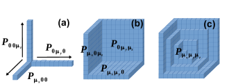
Figure 8: Procedure to calculate the plasmon state population $P_{\mu_{x}\mu_{y}\mu_{z}}$. Panel (a): the edge elements $P_{\mu_{x}00}$, $P_{0\mu_{y}0}$ and $P_{00\mu_{z}}$. Panel (b): the surface elements $P_{\mu_{x}\mu_{y}0}$, $P_{0\mu_{y}\mu_{z}}$ and $P_{\mu_{x}0\mu_{z}}$. Panel (c): the body elements $P_{\mu_{x}\mu_{y}\mu_{z}}$.

In the steady-state of the systems, the time-derivative is zero in Eq. (3) in the main text and the resulting equation leads to a recursion relation for the population, cf. Eq. (4) in the main text. In the following, we explain the procedure to calculate the population with the recursion relation for three modes (one and two modes follow as special cases). First, we assume a fixed value for $P_{000}$ and use it to calculate the edge elements $P_{\mu_{1}00}$, $P_{0\mu_{2}0}$ and $P_{00\mu_{3}}$ with simplified versions of Eq. (4), cf. Fig. 8 (a) :

$$P_{\mu_{1}00} =\frac{\eta_{\mu_{1}00}^{\left(11\right)}P_{\mu_{1}-1,00}}{\left(\gamma_{\mathrm{1}}\mu_{1}+\kappa{}_{\mu}^{\left(1\right)}\right)},$$ (117)

$$P_{0\mu_{2}0} =\frac{\eta_{0\mu_{2}0}^{\left(22\right)}P_{0,\mu_{2}-1,0}}{\left(\gamma_{2}\mu_{2}+\kappa{}_{\mu}^{\left(2\right)}\right)},$$ (118)

$$P_{00\mu_{3}} =\frac{\eta_{00\mu_{3}}^{\left(33\right)}P_{00,\mu_{3}-1}}{\left(\gamma_{3}\mu_{3}+\kappa{}_{\mu}^{\left(3\right)}\right)}.$$ (119)

Secondly, we calculate the surface elements $P_{\mu_{1}\mu_{2}0}$ with the known $P_{\mu_{1}00}$ and $P_{0\mu_{2}0}$ according to a simplified version of Eq. (4), cf. Fig. 8 (b):

$$P_{\mu_{1}\mu_{2}0}=\frac{\sum_{j=1}^{2}\eta_{\mu_{1}\mu_{2}0}^{\left(j1\right)}P_{\mu_{1}-1,\mu_{2},0}+\sum_{j=1}^{2}\eta_{\mu_{1}\mu_{2}0}^{\left(j2\right)}P_{\mu_{1},\mu_{2}-1,0}}{\left(\gamma_{1}\mu_{1}+\kappa{}_{\mu_{1}\mu_{2}0}^{\left(1\right)}\right)+\left(\gamma_{2}\mu_{2}+\kappa{}_{\mu_{1}\mu_{2}0}^{\left(2\right)}\right)}.$$ (120)

Similarly, we can also calculate other surface elements $P_{0\mu_{2}\mu_{3}}$ and $P_{\mu_{1}0\mu_{3}}$ according to simplified versions of Eq. (4):

$$P_{0\mu_{2}\mu_{3}} =\frac{\sum_{j=2}^{3}\eta_{0\mu_{2}\mu_{3}}^{\left(j2\right)}P_{0,\mu_{2}-1,\mu_{3}}+\sum_{j=2}^{3}\eta_{0\mu_{2}\mu_{3}}^{\left(j3\right)}P_{0\mu_{2}\mu_{3}-1}}{\left(\gamma_{2}\mu_{2}+\kappa{}_{0\mu_{2}\mu_{3}}^{\left(2\right)}\right)+\left(\gamma_{3}\mu_{3}+\kappa{}_{0\mu_{2}\mu_{3}}^{\left(3\right)}\right)},$$ (121)

$$P_{\mu_{1}0\mu_{3}} =\frac{\sum_{j=1,3}\eta_{\mu_{1}0\mu_{3}}^{\left(j1\right)}P_{\mu_{1}-1,0,\mu_{3}}+\sum_{j=1,3}\eta_{\mu_{1}0\mu_{3}}^{\left(j3\right)}P_{\mu_{1}0\mu_{3}-1}}{\left(\gamma_{1}\mu_{1}+\kappa{}_{\mu_{1}0\mu_{3}}^{\left(1\right)}\right)+\left(\gamma_{3}\mu_{3}+\kappa{}_{\mu_{1}0\mu_{3}}^{\left(3\right)}\right)}.$$ (122)

Finally, we calculate the body elements $P_{\mu_{1}\mu_{2}\mu_{3}}$ with the known $P_{\mu_{1}\mu_{2}0}$, $P_{0\mu_{2}\mu_{3}}$ and $P_{\mu_{1}0\mu_{3}}$ by applying repeatedly Eq. (4), cf. Fig. 8 (c). The reason why we can achieve the above simplified versions of Eq. (4) is that the rates with $\mu_{j}<0$ will vanish.

To calculate the population of molecular states $P_{g}^{\left(n\right)}=\sum_{\mu}\rho_{g\mu,g\mu}^{\left(n\right)}$, $P_{f}^{\left(n\right)}=\sum_{\mu}\rho_{f\mu,f\mu}^{\left(n\right)}$ and $P_{e}^{\left(n\right)}=\sum_{\mu}\rho_{e\mu,e\mu}^{\left(n\right)}$, we extract $\rho_{g\mu,g\mu}^{\left(n\right)}$,$\rho_{f\mu,f\mu}^{\left(n\right)}$,$\rho_{e\mu,e\mu}^{\left(n\right)}$ from Eqs. (64), (84) and (85) and express them as functions of the plasmon state population $P_{\mu}=\rho_{\mu\mu}$.

$$\rho_{g\mu,g\mu}^{\left(n\right)}=w_{\mu}^{\left(n\right)}\left(k_{e\to g}^{\left(n\right)}t_{\mu}^{\left(n\right)}-k_{e\to f}^{\left(n\right)}r_{\mu}^{\left(n\right)}\right)P_{\mu}$$

$$-k_{f\to e}^{\left(n\right)}w_{\mu}^{\left(n\right)}\sum_{k=1}^{3}\left(u_{\mu}^{\left(kn\right)}t_{\mu}^{\left(n\right)}+r_{\mu}^{\left(n\right)}v_{\mu}^{\left(kn\right)}\right)P_{\mu_{k}-1},$$ (123)

$$\rho_{f\mu,f\mu}^{\left(n\right)}=-w_{\mu}^{\left(n\right)}\left(k_{e\to g}^{\left(n\right)}s_{\mu}^{\left(n\right)}-k_{e\to f}^{\left(n\right)}q_{\mu}^{\left(n\right)}\right)P_{\mu}$$

$$+w_{\mu}^{\left(n\right)}k_{f\to e}^{\left(n\right)}\sum_{k=1}^{3}\left(u_{\mu}^{\left(kn\right)}s_{\mu}^{\left(n\right)}+q_{\mu}^{\left(n\right)}v_{\mu}^{\left(kn\right)}\right)P_{\mu_{k}-1},$$ (124)

$$\rho_{e\mu_{j}-1,e\mu_{j}-1}^{\left(n\right)}=\sum_{k=1}^{3}q_{\mu}^{\left(jkn\right)}\Big{[}k_{f\to e}^{\left(n\right)}P_{\mu_{k}-1}+k_{\mu}^{\left(kn\right)}P_{f\mu}^{\left(n\right)}$$

$$+\left(k_{g\to e}^{\left(n\right)}-k_{f\to e}^{\left(n\right)}-\left(d_{\mu}^{\left(kn\right)}+k_{\mu}^{\left(kn\right)}+\sum_{l=1}^{3}g_{\mu}^{\left(kln\right)}+a_{\mu}^{\left(kn\right)}\right)\right)P_{g\mu}^{\left(n\right)}\Big{]}.$$ (125)

References

(1)Pelton, M.; Aizpurua, J.; Bryant, G. Laser
& Photon. Rev.2008 2, 136-157
(2)Tame, M. S.; McEnergy, K. R.; Özdemir, S. K.; Lee,
J.; Maier, S. A.; Kim, M. S. Nature Physics2013,
9, 329
(3)Ma, R. M.; Oulton, R. F.; Sorger, V. J.; Zhang, X.
Laser Photonics Rev., 2013 1, 1-21
(4)Berini, P.; Leon, I. D. Nat. Photonics2012,
285, 16
(5)Cade, N. I.; Ritman-Meer, T.; Richards, D. Phys.
Rev. B2009,79, 241404
(6)Zelinskyy, Y.; Zhang, Y.; May, V. J. Phys.
Chem. A2012, 116, 11330
(8)Zhang, Y.; Zelinskyy, Y.; May, V. J. Nanopot.2012, 6, 063533
(9)Fleischmann, M.; Hendra, P. J.; McQuillan,
A. J. Chem. Phys. Lett.1947, 26 163-166
(10)Johansson, P.; Xu, H. X.; Käll, M. Phys.
Rev. B2005, 72 035427
(11)Ding, S. Y.; Zhang, X. M.; Ren, B.; Tian, Z. Q.,
Surface-enhanced raman spectroscopy: General introduction,
Encyclopedia of Analytical Chemistry, John Wiley & Sons, Ltd. 2014
(12)Gu, X. F.; Qiu, T.; Zhang, W. J.; Chu, P. K. Nano.
Res. Lett.2011, 6, 199
(13)Gao, N.; Huang, K.; Li, J. C.; Li, S. P.; Yang, X.;
Kang, J. Y. Sci. Rep.2012, 2, 816
(14)Atwater, H. A.; Polman, A. Nat. Materials,
2010, 9, 205-213
(15)Wu, J. L.; Chen, F. C.; Hsiao, Y. S.; Chien, F. C.;
Chen, Peilin; Kuo, C. H.; Huang, M. H.; Hsu, C. S. Acs Nano2011, 5, 959-967
(16) Yin, Y.; Qiu, T.; Li, J.; Chu, P. K. Nano. Energy2012, 1, 25
(17) Bergman, D. J.; Stockman, M. I., Phys. Rev.
Lett.2013, 90, 027402
(18) Noginov, M. A.; Zhu, G.; Belgrave, A. M. et al,
Nature2009, 460, 1110
(19) Ho, J.; Tatebayashi, J.; Sergent, S.; Fong, C. F.;
Ota, Y.; Iwamoto, S.; Arakawa, Y. Acs Photonics2015,
2, 165
(20) Oulton, R. F.; Sorger, V. J.; Zentgraf, T.; Ma,
R. M.; Gladden, C.; Dai, L.; Bartal, G.; Zhang, X. Nature2009,
461, 629
(21) Wu C. Y. ; Kuo, C. T.; Wang, C. Y.; et al., Nano
Lett. 2011, 11, 4256
(22) Lu, Y. J.; Kim, J.; Chen, H. Y.; et al., Science2012, 337, 450
(23) Lu, Y. J.; Yang, C. Y.; J. Kim, et al, Nano
Lett.2014, 14, 4381
(24) Hou, Y.; Renwick, P.; Liu, B.; Bai J.; Wang, T. Sci.
Rep. 2014, 4, 5014
(25) Zhang, Q.; Li, G. Y.; Liu, X. F.; Qian, F.; Li,
Y.; Sum, T. C.; Lieber C. M.; Xiong, Q. H. Nature Comm.2014
5, 4953
(26)Sidiropoulos, T. P. H.; Röder, R.; Geburt, S.; Hess,
O.; Maier, S. A.; Ronning, C.; Oulton, R. F., Nature Physics,
2014, 10, 870
(27)Chou, Y. H.; Chou, B. T.; Chiang, C. K.; Lai, Y.
Y.; Yang, C. T.; Li, H.; Lin, T. R.; Lin, C. C.; Kuo, H. C.; Wang,
S. C.; Lu, T. C. Acs Nano2015, 9, 3978
(28)Chou, B. T.; Chou, Y. H.; Wu, Y. M.; Chung, Y. C.;
Hsueh, W. J.; Lin, S. W.; Lu, T. C.; Lin, T. R.; Lin, S. D. Sci.
Rep.2016, 6, 19887
(29) Ma, R. M.; Oulton, R. F.; Sorger, V. J.; Bartal, G.;
Zhang, X. Nature Mat.2011, 10, 110
(30)Ma, R. M.; Yin, X. B.; Oulton, R. F.; Sorger, V.
J.; Zhang, X. Nano. Lett.2012, 12, 5396-5402
(31) Hill, M. T.; Marell, M.; Leong, E. S. P.; et al.,
Opt. Express2009, 17, 11107
(33) Kwon, S. H.; Kang, J. H.; Seassal, C.; Kim, S. K.;
Regreny, P.; Lee, Y. H.; Lieber, C. M.; Park, H. G. Nano. Lett.
2010, 10, 3679
(34)Lee, J. H.; Khajavikhan, M.; Simic, A.; Gu, Q.; Bondarenko,
O.; Slutsky, B.; Nezhad, M. P.; Fainman, Y. Opt. Express2011,
19, 21524
(35)Khajavikhan, M.; Simic, A.; Katz, M.; Lee, J. H.; Slutsky,
B.; Mizrahi, A.; Lomakin, V.; Fainman, Y. Nature2012,
482, 204-207
(36) Ding, K.; Liu, Z. C.; Yin, L. J.; et al., Phys.
Rev. B2012, 85, 041301 (R)
(37)Matsudaira, A.; Lu, C. Y.; Zhang, M.; Chuang,
S. L.; Bimerg, D. IEEE Photonics2012, 4, 1103-1114
(38)Lu, C. Y.; Ni, C. Y.; Zhang, M.; Chuang, S. L.; Bimberg,
D. H. IEEE, 2013, 19, 1077
(39)Lu. C. Y.; Chuang, S. Lien; Bimberg, D. IEEE,
2013, 49, 114
(40)Chang, S. W.; Lu, C. Y.; Chuang, S. L.; German,
T. D., Pohl, U. W. Bimberg, D. IEEE2011, 17, 1681-1692
(41) Suh, J. Y.; Kim, C. H.; Zhou, W.; Huntington, M.
D.; Co, D. T.; Wasielewski, M. R.; Odom, T. W. Nano Lett.2012,
12, 5769-5774
(42) Zhou, W.; Dridi, M.; Suh, J. Y.; Kim, C. H.; Co,
D. T.; Wasielewski, M. R.; Schatz, G. C.; Odom, T. W. Nature
Nanotech.2013, 8, 506
(43) Yang, A.; Hoang, T. B.; Dridi, M.; Deeb, C.; Mikkelsen,
M. H.; Schatz, G. C.; Odom, T. W. Nature Comm. 2015,
6, 1-7
(44) Yang, A.; Li, Z. Y.; Knudson, M. P.; Hryn, A. J.;
Wang, W. J.; Aydin, K.; Odom, T. W. Acs. Nano. 2015,
9, 11582-11588
(45)Schokker, A. H. ; Koenderink, A. F.; Acs
Photonics2015, 2, 1289-1297
(46)Chang, S. W.; Lin, T. R.; Chuang, S. L. Opt.
Express2010, 18, 15039-15053
(47)Li, N.; Liu K.; Sorger, V. J.; Sadara, D. K. Sci.
Rep.2015, 5, 14067
(48) Richter, M.; Gegg, M.; Theuerholz, T. S.; Knorr,
A. Phys. Rev. B2015, 91, 035306
(49)Parfenyev, V. M.; Vergeles, S. S. Opt. Express
2014, 22, 13571
(50) Sargent II, M.; Scully, M. O.; Lamb, W. E. Laser
Physics, Addison-Wesley Publishing Company, Reading, Masschusetts,
et al.,1974
(51) Zhang, Y.; May, V. J. Chem. Phys.2015,
142, 224702
(52) Zhang, Y.; Mølmer, K.; May, V. Phys. Rev.
B2016, 94, 045412
(53)Savage, K. J.; Hawkeye, M. M.; Esteban, R.; Borisov,
A. G.; Aizpurua, J.; Baumberg, J. J. Nature, 2012,
491, 574
(54) Zhang, Y.; May, V. Phys. Rev. B2014,
89, 245441
(55)Gersten, J.; Nitzan, A. J. Chem. Phys.1981,
75, 1139
(56)Weick, G.; Molina, R. A.; Weinmann, D.; Jalabert,
R. A. Phys. Rev. B2005, 72, 115410
(57) The three molecular states do not need to be electronic
states. They can also be the relevant electronic-vibrational states in dye molecules.
(58) Although the gold nano-sphere can locally enhance
an off-resonant incoming field, the enhancement is often very
weak. Therefore, here, we assume an homogeneous driving field
in the small region of the nano-laser.
(59) Scully, M. O.; Zubairy, M. S. Quantum Optics,
Cambridge University Press, Cambridge, 2001
(60) Zhang, Y.; May, V.; Mølmer, K. Emission
Narrowing without Lasing and Quantum Interference Effect in a Plasmonic
Nano-laser, in preparation
(61) Haken, H. Laser Theory, Springer-Verlag Berlin,
Heidelberg, New York, Tokyo, 1984
(62) Meng, X. G.; Kildishev, A. V.; Fujita, K. et al.,
Nano Lett.2013, 9, 4106