∎
22email: benjamin.ambrosio@univ-lehavre.fr
Propagation of bursting oscillations in coupled non-homogeneous Hodgkin-Huxley Reaction-Diffusion systems
Abstract
In this paper, we consider networks of reaction-diffusion systems of Hodgkin-Huxley type. We give a general mathematical framework, in which we prove existence and unicity of solutions as well as the existence of invariant regions and of the attractor. Then, we illustrate some relevant numerical examples and exhibit bifurcation phenomena and propagation of bursting oscillations through one and two coupled non-homogeneous systems.
Keywords:
Complex Dynamical Systems Hodgkin Huxley Equations Reaction Diffusion Systems1 Introduction
Action potential propagation is a crucial phenomenon for information process in the nervous system and particularly in the brain. One of the paradigmatic models, which has been proposed to describe action potential propagation, is the Hodgkin-Huxley model. Written initially in 1952, see HH , for the description of the electrical activity of the squid giant axon, its formalism has served as basis of number of models widely used in Mathematical Neuroscience, see for example Ambrosio0 ; Ambrosio1 ; Ambrosio2 ; C1 ; Fitz ; Hin ; Mor ; Nagumo and references therein cited. At that time, Hodgkin and Huxley used the new voltage clamp technique to maintain constant the membrane potential. This technique allowed them to elaborate and fit the functional parameters of their model of four ODEs with their experiments. Basically, the model is obtained by considering the cell as an electrical circuit. The membrane acts as a capacitor whereas ionic currents result from ionic channels acting as variable voltage dependent resistances. The model takes into account three ionic currents: potassium (), sodium () and leakage (mainly chlorure, ). The Hodgkin-Huxley (HH) system reads as:
| (1) |
where subscript stands for derivative and where is the external membrane current, is the membrane capacitance, are respectively the maximal conductances and the (shifted) Nernst equilibrium potentials. The functions and describe the transition rates between open and closed states of channels. They read as:
| (2) |
The (shifted) Nernst equilibrium potentials are given by:
These values are taken from Izh , p 37-38, and correspond to those of the Hodgkin-Huxley original paper HH , after a change of variables . Recall that the Nernst equilibrium potentials are obtained by solving, for each ion the equation:
where and are concentrations of the ions inside and outside the cell. is the universal gas constant, is temperature in Kelvin, is the Faraday’s constant, is the valence of the ion. For example, this computation gives for sodium, with , , (see Izh p 50):
which with a shift of gives the value of used here. Originally, Hodgkin and Huxley used the shift to obtain a potential at rest of approximately . Before going into more theoretical aspects, we give some interpretation about the form of conductances. The proportion of open potassium channels is . This comes from the fact that opening gates of potassium are required to open the potassium channel. Hence, the gives the probability of the gate to be in active state and results in the term for potassium. For the sodium, it is supposed that there are there are three gates which open the channels and one which close them. Hence, the proportion of sodium opened channels is given by , where it is supposed that stands for the probability of sodium opening gates to be active while stands for probability of sodium closing gates to be active. For more details on various aspects of the HH model, we refer to Cro ; Erm ; Izh and the original paper HH . In the present paper, we consider a general network of reaction-diffusion (RD) HH equations. Note that the study of networks of reaction-diffusion systems start to attract an increasing number of mathematical analysis, see for example, Ambrosio1 ; Ambrosio2 ; Yang . They appear naturally in the neuroscience context. The general network reads as:
| (3) |
in a bounded domain and with Neumann boundary conditions and where,
| (4) |
with
| (5) |
and .
The functions represent excitatory nonlinear coupling (i.e. chemical synaptic coupling) between neurons, see Ambrosio3 ; Ambrosio4 ; Bel ; C1 and
references therein cited.
Without loss of generality, we have set the constant equal to . Hence, the value allows the neuron to receive an excitatory input each time
one of his
presynaptic neurons crosses the treshold value . The value , implies that approximates the Heaviside function.
The Neumann condition is chosen here to not induce boundary effects. Here, and are regular non negative bounded function of .
Our first aim is to provide a mathematical framework for solutions of system (3). This is done in section 2. We prove the global existence
of solutions as well as the existence of invariant regions and the existence of an attractor.
Then, in the third section, we deal with numerical simulations for a single non-homogeneous HH RD system and two coupled HH RD systems.
In this last part, we exhibit some relevant bifurcation phenomena and propagation of bursting oscillations from first neuron to the second neuron.
Note that system (3) is autonomous, which means that the bursting oscillations are generated here without external driving component as in
Ambrosio0 . See also Cle .
2 Mathematical Framework
2.1 Existence of the solution
Let the space of continuous functions defined on the real interval . We start with the proof of the existence of the solution of (3). The proof is divided into four parts. First, we prove the local existence and uniqueness of a mild-solution, thanks to a fixed point theorem. Then, we prove the regularity of this mild solution. Finally, we prove the bounds for as well as the global existence.
Theorem 2.1
For all initial conditions such that , , there exists a unique solution of (3). Furthermore, and for all , .
Proof
It is known that the equation
with
generates an analytical semigroup on , see Lunardi , Theorem 3.1.22 p 98. Let us denote by this semigroup. The first step is to look for mild solutions of (3). Mild-solutions are solutions of the variation of constants formula of (3), and written with the semigroup notation. The general network equation for mild-solutions reads as:
| (6) |
where:
| (7) |
The local existence follows by application of the fixed point theorem, to the function:
defined by the right-hand side of (6), in which we fix the initial condition (below, for sake of simplicity, we drop the subscript on ). Let denote the function . For all , the ball of center and radius in , we have, for fixed
where stands here for the sup norm on and where is a constant depending on which comes from the boundedness theorem. We have also used the property of the linear semigroup : and , see Lunardi p 35. It follows that, for , . By analog computations, we prove that
which proves that for , is a contraction mapping.
Therefore, has a unique fixed point which provides the existence and uniqueness of the local mild solution.
Now, we deal with the regularity. We already know, that, solutions belong to .
Since the term, does not complicate the proof, without loss of generality, we drop the subscript .
A computation shows that the quantity
is well defined, for , as and that the resulting function is contiuous on . For , the derivative may not exist,
since admits a limit as if and only if . For functions and the same computation shows that they
belong to . Hence, the regularity statement follows.
Now, we deal with the global existence.
First, we prove that and remain in . Without loss of generality, we drop the subscript and consider only the variable.
It satisfies,
Let
Then,
with and .
It follows that:
Also,
Then, the global existence follows from the inequality,
which comes from the first equation of (3) and which by Gronwall inequality yields:
2.2 Existence of an invariant region
We assume that the values of parameters are as specified in (2) and (5). This implies in particular that are . We also assume that 111We can drop this last asumption. In this case, the upper bound of the invariant region for is replaced by ..
Theorem 2.2
We assume that , and , then and ,
Proof
We have already proved that . To prove we use the following argument. Let the first time that reaches the value at the point , then which implies since all the other terms are non negative and . Analogously, let the first time that reaches the value at the point then which implies since all the other terms are non positive and .
2.3 Existence of an attractor
We denote by . In this section, we use the framework of Tem to establish the existence of an invariant, compact and connected set which attracts all tre trajectories starting in . We first recall the definition of the limit set. We denote by the semi-group associated with equation (3).
Definition 1
For , we define the set of by:
and similarly the set of by:
The following theorem holds.
Theorem 2.3
Let
Then is a nonempty invariant, compact and connected set in . Furthermore, for all initial condition in , the solution of (12) starting at verifies:
Proof
We use the framework of Tem . Hence, we need to establish some compacity on trajectories. For convenience, we drop the subscript . For variable , without loss of generality, we write
| (8) |
since the coupling term does not change the proof arguments. We prove that , is compact in , for some . By Ascoli’s theorem, it is sufficient to prove the equicontinuity of
for some . Then, we deal with variable . For, variables the same arguments apply. We prove that:
where
and
According to Tem , this suffices to prove theorem 2.3. Let us start with . Recall that for all , . Now, we establish a bound on . For all it holds,
since we assume . It follows that
and that:
| (9) |
with , where denotes the norm in the Sobolev space and denotes the norm in the Lebesgue space . Note that inequality (9), is actually a particular case of Agmon-Douglis-Niremberg estimates, see Lunardi p 72 and AgDoNi . However, since we consider here the 1-dimensional case the proof is much more simpler. Next, we adapt some arguments from Har . First, note that the following classical inequalities hold:
and
for some generic constants , see Lunardi p 35. This implies that:
Now, let , and such that:
| (10) |
for example, we can choose , and . Then, we have ,see Har and also Henry ,
Finally, we obtain that for all :
Applying this result in (8) implies:
| (11) |
where comes from the fact that remain in . This implies that
where the constant depends on but not on , neither in . This proves the equicontinuity of
Now, we deal with . We compute,
we obtain (for convenience, we only write the dependence on and ),
which by integration leads to
where and is a generic constant. This gives the announced statement.
Remark 1
The difficult point in the proof was to obtain the bound (11).
3 Bifurcations and propagation of oscillations in one and two coupled non-homogeneous neurons
3.1 Bifurcation in a single non-homogeneous neuron
In this section, we deal with equation (3) with . It reads:
| (12) |
We have proceeded to numerical simulations in the domain , on time interval , using our own C++ program with a uniform finite difference scheme in space and a Runge-Kutta method integration in time. Hence, the space-mesh reads, , and the time-mesh reads, Note that since the equation for the potential is linear in and the equation for channels are linear in . One can, from step to step, compute for fixed . And use a similar argument for computation. A discussion on this aspects can be found in Bal . The particularity is that we choose a regular non homogeneous , approximating the discontinuous function defined by:
| (13) |
In the following descriptions, for simplicity we identify with . We will use the same convention for on section 3.2.
We emphasize here three different regimes corresponding to different region of parameter value .
Stationary and periodic solutions for
Convergence toward stationary solution for
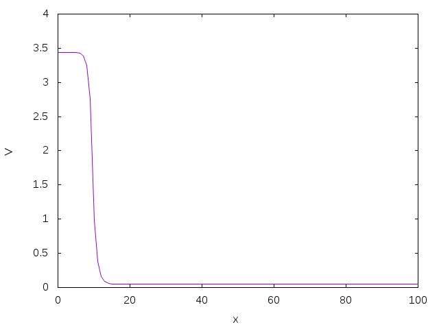
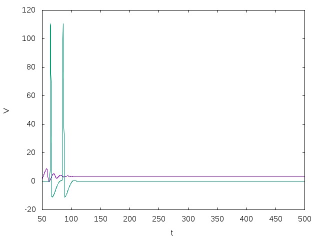
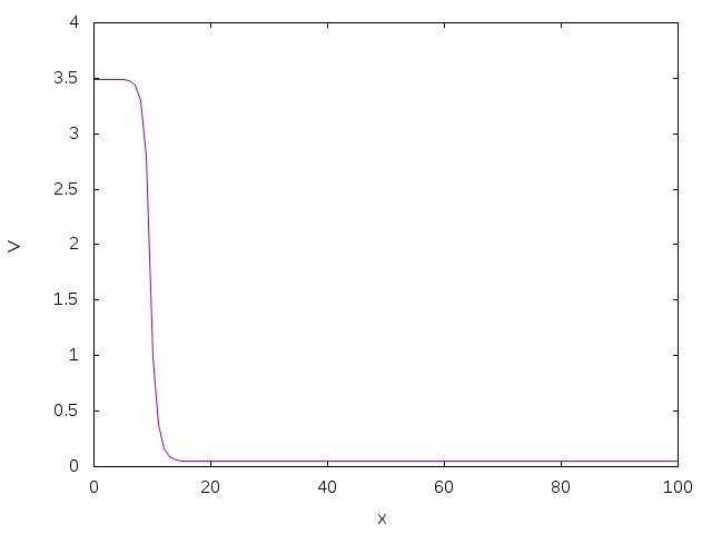
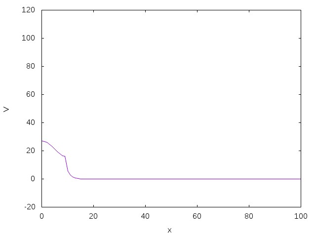
For several initial conditions and for small , i.e. for ,
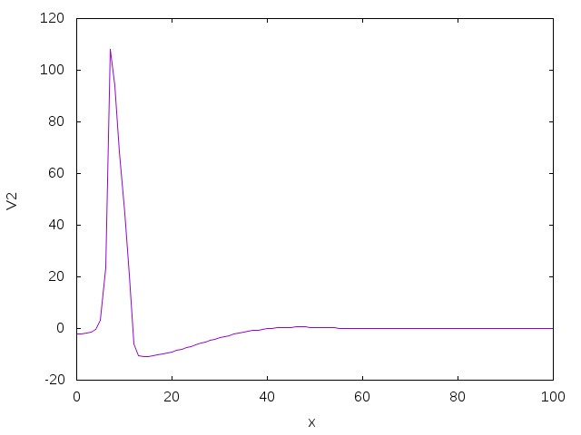
we obtain asymptotically a convergence toward a steady state. In figure 1, we have illustrated this phenomenon for , for initial condition .
The first panel illustrates the stationary space dependent solution, which is attained asymptotically.
The second panel illustrates the time evolution for and .
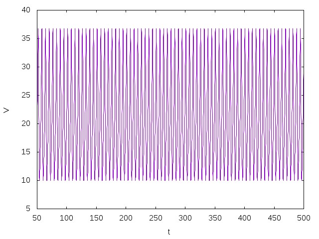
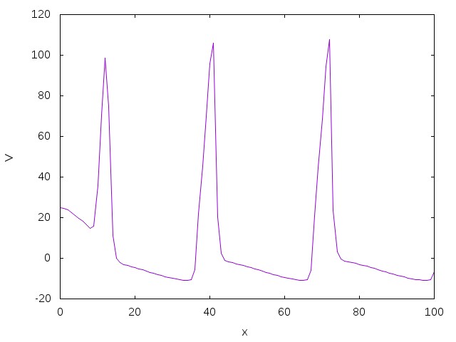
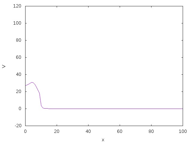
Convergence toward periodic solution for
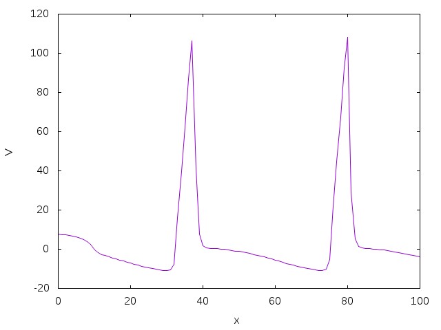
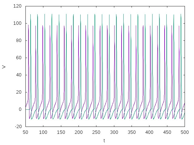
For the same initial conditions as before and for , we obtain asymptotically a convergence toward a periodic solution.
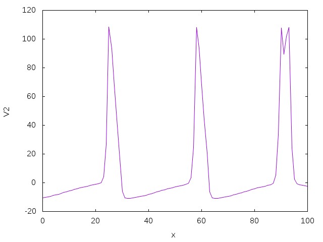
This periodic solution consists of large solutions starting at and propagating form left to right.
We have illustrated this phenomenon in figure 2, for initial condition .
The first panel illustrates the propagation of oscillations from left to right. In fact, it shows the solution along the space for a fixed time .
As in the previous figures, the second panel illustrates the time evolution for and . It shows periodic solutions.
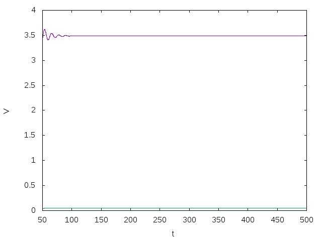
Convergence toward stationary solution for
We note for this value the coexistence of attractive stationary and periodic solutions. Indeed, for , and initial condition , we observe
a convergence toward a stationary solution. The phenomenon is depicted as before in figure 3.
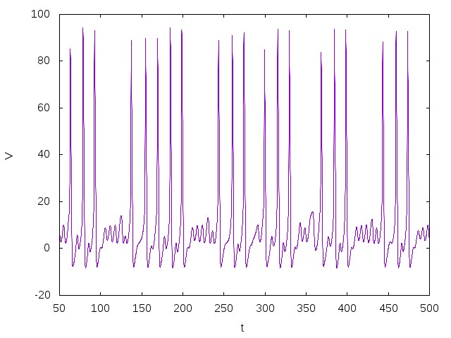
Propagation of busting oscillations
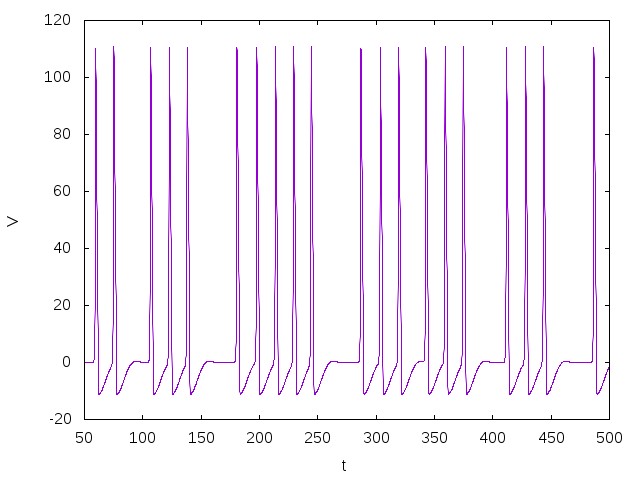
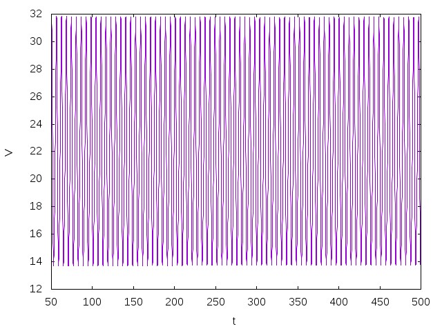
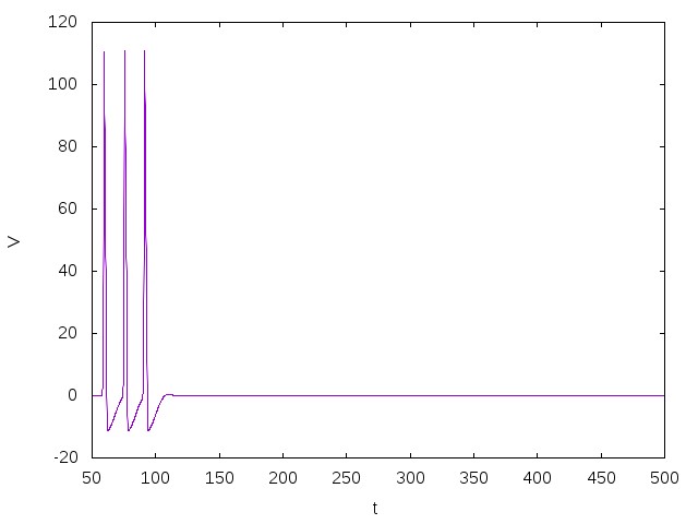
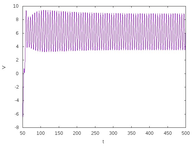
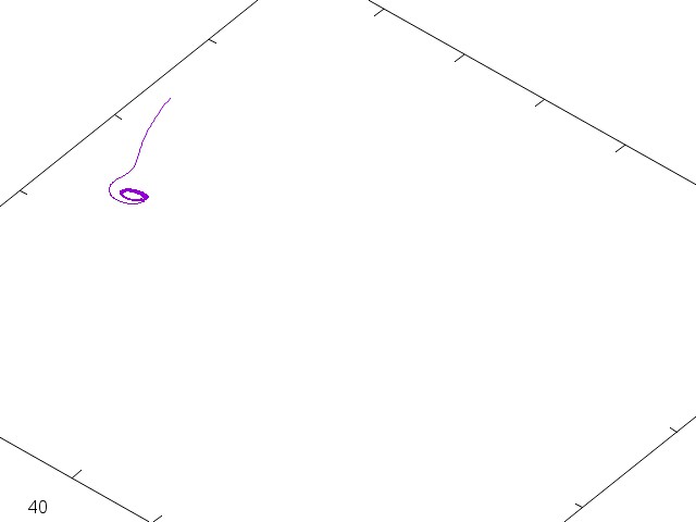
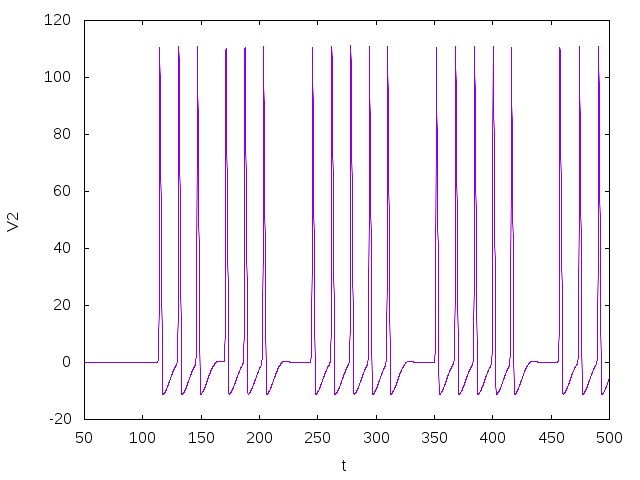
Convergence toward a solution with propagation of busting oscillations for
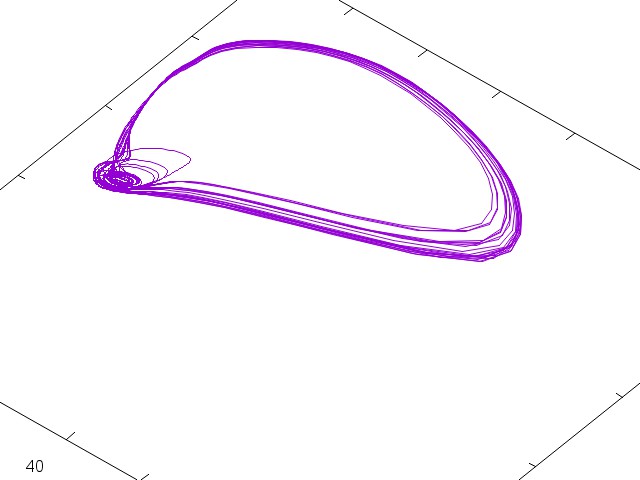
For , we observe propagation of busting oscillations. The left cells oscillate continuously, but not all the oscillations propagate trough the right-cells. In fact, the right-cells alternate quiescent phases with oscillating phases, which is a bursting phenomenon. We illustrate this phenomena in figure 4. The left-top panel illustrates the time evolution at . We observe oscillations. The right-top panel illustrates the time evolution at . We observe bursting phenomena. The left-middle panel illustrates the time evolution at . We observe the so-called mixed-mode oscillations: an alternation of small and large oscillations. The right-middle panel illustrates the time evolution at , in the (V,n,m) variables. The left-down panel illustrates the propagation of oscillations in space at fixed time . The right-down panel illustrate the quiescent phase in space at fixed time .
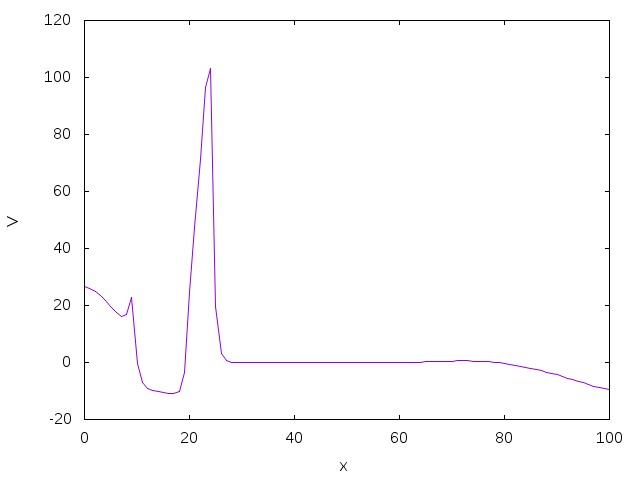
Death-spot
Convergence toward a solution with death-spot
For , we observe this another interesting phenomenon. The left cells oscillate continuously, but the wave propagation fails to propagate along the whole space. This is known as the death-spot phenomena, see Ambrosio0 ; Yan1 ; Yan2 and references therein cited. The right cells seem to have reached a stationary state whereas the left cells are still oscillating. The left-top panel illustrates the time evolution at . We observe oscillations. The right-top panel illustrates the time evolution at . We observe a near-stationary solution. The left-middle panel illustrates the time evolution at . We observe small oscillations. The right-middle panel illustrates the time evolution at , in the (V,n,m) variables. The left-down panel illustrates the oscillations of left cells and the near stationary state for right cells in space at fixed time and time .
3.2 Propagation of bursting oscillations in 2 coupled neurons
In this section, we deal with equation (3) with , , for and,
| (14) |
It reads:
| (15) |
We have proceeded to numerical simulations as before with
| (16) |
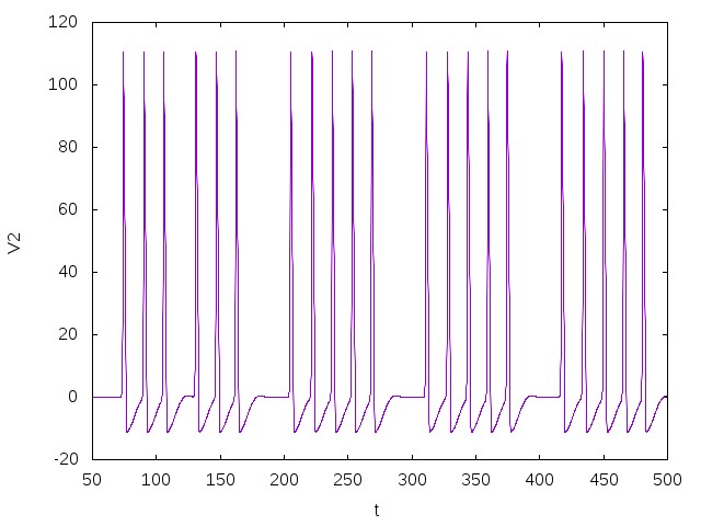
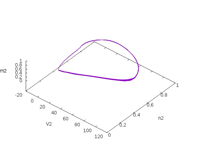
As the neuron is not affected by the coupling, the dynamic of this neuron has already been described. For the second neuron, we observe the propagation of bursting oscillations from neuron to neuron . As the coupling acts only on the right side of the neuron , oscillations propagate from right to left. It is interesting to note that there is also a short propagation toward the right boundary. We can observe this on the spike with a double head at the right side on the right-down panel of figure 6.
4 Conclusion
In this paper, we have considered a general network of HH RD systems. We have proved existence and uniqueness of solutions as well as the existence of invariant region and of the attractor in the space of continuous functions. We have also exhibited bifurcation phenomena and propagation of bursting oscillations along one and two coupled neurons. These numerical results show that a rich behavior may be obtained thanks to the space-inhomogeneities. In future works, we aim to develop theoretical tools to describe and analyze these phenomena.
Acknowledgments
The authors would like to thank Région Normandie and FEDER XTERM for financial support.
References
- (1) S. Agmon, A. Douglis and L. Niremberg , Estimates Near the Boundary For Solutions of Elliptic Partial Differential Equations Satisfying general Boundary conditions, Communication on Pure and Applied Mathematics, 12 (1959) 623-727.
- (2) B. Ambrosio and J-P. Françoise, Propagation of Bursting Oscillations, Phil. Trans. R. Soc. A.,(2009) 4863-4875.
- (3) B. Ambrosio and M.A. Aziz-Alaoui, Synchronization and control of coupled reaction-diffusion systems of the FitzHugh-Nagumo-type, Computers and Mathematics with Applications 64 (2012) 934-943.
- (4) B. Ambrosio and M.A. Aziz-Alaoui, Synchronization and control of a network of coupled reaction-diffusion systems of generalized FitzHugh-Nagumo type, ESAIM: Proceedings and surveys, March 2013, Vol. 39, p. 15-24.
- (5) B. Ambrosio, M.A. Aziz-Alaoui and and V.L.E Phan, Attractor of complex networks of Reaction-Diffusion systems of FitzHugh-Nagumo type, under review, arXiv:1504.07763v2
- (6) B. Ambrosio, M.A. Aziz-Alaoui and V.L.E Phan, Large time behavior and Synchronization for complex networks of Reaction Diffusion systems of FitzHugh-Nagumo type, under review, arXiv:1504.07763v2
- (7) A. Balti, Modélisation mathématique et analyse de réseaux complexes d’interaction de Hodgkin-Huxley, application en neuroscience, PhD Thesis, Le Havre Normandie University, 2016.
- (8) I. Belykh, E. De Lange, M. Hasler, Synchronization of bursting neurons: What matters in the network topology, Phys. Rev. Lett. 188101, 2005.
- (9) N. Corson, M.A. Aziz-Alaoui, Asymptotic dynamics of the slow-fast Hindmarsh-Rose neuronal system, Dyn. Contin. Discrete Impuls. Syst. Ser. B, 16 (2009),535-549.
- (10) F. Clement and J-P. Françoise, Mathematical Modeling of the GnRH Pulse and Surge Generator, SIAM J. Appl. Dyn. Syst.,(2005) 6(2) 441–456.
- (11) J. Cronin, Mathematical aspects of Hodgkin-Huxley neural theory, Cambridge University Press, 1987.
- (12) D. Henry, Geometric Theory of Semilinear Parabolic Equations, Springer, 1981.
- (13) G.B. Ermentrout, D.H. Terman, Mathematical Foundations of Neurosciences, Springer, 2009.
- (14) R. A. FitzHugh, Impulses and physiological states in theoretical models of nerve membrane, Biophys. J. 1, (1961) 445-466.
- (15) A. Haraux et M. Kirane, Estimations por des problèmes paraboliques semi-linéaires, Annales de la faculté des science de Toulouse, 5 (1983), p. 265-280.
- (16) J. L. Hindmarsh and R. M. Rose, A model of neuronal bursting using three coupled first order differential equations, Proc. R. Soc. London, Ser. B, 221 (1984) 87-102.
- (17) A.L. Hodgkin and A.F. Huxley, A quantitative description of membrane current and its application to conduction and excitation in nerve, J. Physiol. 117 (1952) 500-544.
- (18) E.M. Izhikevich, Dynamical Systems in Neuroscience: The Geometry of Excitability and Bursting, The MIT Press, 2005.
- (19) A.Lunardi, Analytic semigroup and optimal regularity in parabolic problems, Birkhauser, 1995.
- (20) C. Morris and H. Lecar, A Voltage oscillations in the barnacle giant muscle fiber, Biophys. J., B 35(1981)193-213.
- (21) J. Nagumo, S. Arimoto and S. Yoshizawa, An active pulse transmission line simulating nerve axon, Proc. IRE. 50 (1962) 2061-2070.
- (22) R. Temam, Infinite Dimensional Systems in Mechanics and Physics, Springer-Verlag, 1988
- (23) T. Yanagita, Y. Nishiura, and R. Kobayashi, Signal propagation and failure in one dimensional FitzHugh-Nagumo equations with periodic stimuli, Physical Review E, 71 :36226, 2005.
- (24) T. Yanagita, Y. Nishiura, and R. Kobayashi, Resonance and the formation of deathspot in one-dimensional FitzHugh-Nagumo equations, Progress of Theoretical Physics Supplement, 161 :393-396, 2006.
- (25) X. Yang, J. Cao, and Z. Yang, Synchronization of coupled reaction-diffusion neural networks with time varying delays via pinning-impulsive controller, SIAM Journal on Control and Optimization, 51(5) (2013) 3486-3510.