Transport of power in random waveguides with turning points

Abstract

We present a mathematical theory of time-harmonic wave propagation and reflection in a two-dimensional random acoustic waveguide with sound soft boundary and turning points. The boundary has small fluctuations on the scale of the wavelength, modeled as random. The waveguide supports multiple propagating modes. The number of these modes changes due to slow variations of the waveguide cross-section. The changes occur at turning points, where waves transition from propagating to evanescent or the other way around. We consider a regime where scattering at the random boundary has significant effect on the wave traveling from one turning point to another. This effect is described by the coupling of its components, the modes. We derive the mode coupling theory from first principles, and quantify the randomization of the wave and the transport and reflection of power in the waveguide. We show in particular that scattering at the random boundary may increase or decrease the net power transmitted through the waveguide depending on the source.

1 Introduction

Guided waves have been studied extensively due to their numerous applications in electromagnetics [13], optics and communications [27, 29], quantum waveguides [17], ocean acoustics [32], etc. The classic waveguides, with straight boundaries and filled with media that are either homogeneous or do not vary along the direction of propagation of the waves, are well understood. The wave equation in such waveguides is separable and the solution is a superposition of independent modes, which are propagating and evanescent modes and, in the case of penetrable boundary, radiation modes. When the geometry of the waveguide varies, or the medium filling it is heterogeneous, the modes are coupled. Examples of mathematical studies that account for mode coupling and lead to numerical methods that model such waveguides can be found in [11, 12, 15, 14, 23]. We are interested in mode coupling due to small random perturbations of the waveguide, which can be quantified more explicitly using asymptotic analysis.

Random models are useful for waveguides with rough boundaries and filled with composite media that vary at small scale, comparable to the wavelength. Such variations are typically small and unknown, so they introduce uncertainty in the model of wave propagation. The random models of the boundary and the wave speed are used to quantify how this uncertainty propagates to the uncertainty of the solution of the wave equation. This is useful information in applications like imaging [10, 7, 9, 2]. The mode coupling theory in waveguides filled with random media has been developed in [24, 16, 19, 21, 20] for sound waves and in [27, 4] for electromagnetic waves. The theory has also been extended to waveguides with random perturbations of straight boundaries [5, 7, 22].

In this paper we develop a mode coupling theory in random waveguides with turning points. We consider for simplicity a two-dimensional acoustic waveguide with sound soft boundary, but the theory can be extended to three dimensions and to electromagnetics. The waveguide has a slowly bending axis, a slowly changing opening and a randomly perturbed boundary. The slow variations occur on a long scale with respect to the wavelength, whereas the random perturbations are at a scale similar to the wavelength.

In the absence of the random perturbations, waves in slowly changing waveguides can be analyzed with a local decomposition in modes that are approximately independent [3, 31]. This is known as the adiabatic approximation [29, Section 19-2], and the result differs from that in waveguides with straight boundaries in one important aspect: The change in the opening of the waveguide causes the number of propagating modes to increase or decrease by $1$ at locations called turning points. Modes transition there from propagating to evanescent or the other way around, and due to energy conservation, the impinging propagating mode is turned back i.e., is reflected. Turning waves in slowly changing waveguides are studied mathematically in [6]. A recent study of their interaction with a random boundary is given in [8], for the case of weak random fluctuations that affect only the turning modes. Here we extend the results in [8] to stronger fluctuations, that couple all the waveguide modes.

Starting from the wave equation, and using the separation of scales of variation of the waveguide, we derive an asymptotic model for the wave field that accounts for coupling of all the modes, propagating and evanescent. This coupling is described by a stochastic system of differential equations for the random mode amplitudes, endowed with initial conditions that model the source excitation and radiation conditions. The excitation is due to a point source, but due to the linearity of the equation, other source excitations can be handled by superposition. We obtain an extension of the diffusion approximation theorem proved in [28] to carry out the asymptotic analysis of the mode amplitudes. The result simplifies when the random fluctuations are smooth, because the forward and backward going components of the propagating modes become independent. This is known as the forward scattering approximation, and applies to propagation between the turning points. At the turning points there is strong coupling of the components of the turning waves, described by random reflection coefficients. With the diffusion approximation theorem, and in the forward scattering approximation regime, we quantify the net effect of the random boundary on the transmitted and reflected power in the waveguide. This is the main result of the paper, and shows that the random boundary can be useful for increasing the transmitted power.

The paper is organized as follows: We begin in section 2 with the formulation of the problem, and the derivation of the asymptotic model for the wave field. Then we give in section 3 the mode decomposition and derive a closed system of stochastic differential equations for the random amplitudes of the propagating modes between turning points. These equations are complemented by source excitation conditions, radiation conditions, as well as continuity and reflection conditions at the turning points. The asymptotic limit of the solution of these equations and the forward scattering approximation are in section 4. We use these results to quantify the transmitted and reflected power in the waveguide in section 5. The diffusion approximation theorem used to carry the asymptotic limit is stated and proved in section 6. We end with a summary in section 7.

2 Formulation of the problem

In this section we give the mathematical model for time-harmonic waves in a random waveguide with variable cross-section and bending axis. We begin in section 2.1 with the setup, and describe the scaling in section 2.2 in terms of a small, dimensionless parameter $\varepsilon$. We use it in section 2.3 to write the wave problem in a form that can be analyzed in the asymptotic limit $\varepsilon\to 0$.

2.1 Setup

Fig. 1: Illustration of a waveguide with slowly varying width $D$ and bending axis parametrized by the arc length $z$. The boundary $\partial\Omega$ is the union of the curves $\partial\Omega^{-}$ (the bottom boundary) and $\partial\Omega^{+}$ (the top boundary). The top boundary is perturbed by small random fluctuations. The unit tangent to the axis of the waveguide is denoted by ${\bm{\tau}}$ and the unit normal ${{\itbf n}}$ points toward the upper boundary. The source of waves is at ${{\itbf x}}_{\star}$.

We consider a two-dimensional acoustic waveguide with sound-soft boundary. The waveguide occupies the semi-infinite domain $\Omega$, bounded above and below by two curves $\partial\Omega^{+}$ and $\partial\Omega^{-}$, as shown in Figure 1. The top boundary $\partial\Omega^{+}$ is perturbed by small random fluctuations about the curve $\partial\Omega^{+}_{o}$ shown in the figure with the dotted line. The axis of the waveguide is at half the distance $D$ between $\partial\Omega_{0}^{+}$ and $\partial\Omega^{-}$. It is a smooth curve parametrized by the arc length $z\in\mathbb{R}$, that bends slowly, meaning that its tangent ${\bm{\tau}}(z/L)$ and curvature $\kappa(z/L)$ vary on a scale $L$ which is large with respect to the waveguide width $D(z/L)$. The width function $D$ has bounded first two derivatives, and to avoid complications in the analysis of scattering of the waves at the random boundary, we also assume that it is monotonically increasing.

Because of the changing geometry, it is convenient to use orthogonal curvilinear coordinates with axes along ${\bm{\tau}}(z/L)$ and ${{\itbf n}}(z/L)$, where ${{\itbf n}}$ is the unit vector orthogonal to ${\bm{\tau}}$, pointing toward the upper boundary. For any ${{\itbf x}}\in\Omega$, written henceforth as ${{\itbf x}}=(r,z)$, we have

$${{\itbf x}}={{\itbf x}}_{\parallel}(z)+r{{\itbf n}}\Big{(}\frac{z}{L}\Big{)},$$ (1)

where ${{\itbf x}}_{\parallel}(z)$ is along the waveguide axis at arc length $z$, satisfying

$$\partial_{z}{{\itbf x}}_{\parallel}(z)={\bm{\tau}}\Big{(}\frac{z}{L}\Big{)},$$ (2)

and $r$ is the coordinate in the normal direction. The domain $\Omega$ is the set

$$\Omega=\{(r,z):~{}z\in\mathbb{R},~{}r\in(r^{-}(z),r^{+}(z))\},$$ (3)

where

$$r^{-}(z)=-\frac{D(z/L)}{2},$$ (4)

is at the bottom boundary $\partial\Omega^{-}$ and

$$r^{+}(z)=\frac{D(z/L)}{2}\left[1+1_{(-Z_{M},Z_{M})}(z)\,\sigma\nu\Big{(}\frac{z}{\ell}\Big{)}\right],$$ (5)

is at the randomly perturbed top boundary $\partial\Omega^{+}$. The perturbation is modeled by the random process $\nu$ and it extends over the interval $(-Z_{M},Z_{M})$, the support of the indicator function $1_{(-Z_{M},Z_{M})}(z)$, where $Z_{M}>L$ is a long scale needed to impose outgoing boundary conditions on the waves. We let the boundaries of the waveguide be straight and parallel for $|z|>Z_{M}$.

The random process $\nu$ is stationary with zero mean

$$\mathbb{E}\big{[}\nu(\zeta)\big{]}=0,$$ (6)

and auto-correlation function

$$\mathcal{R}(\zeta)=\mathbb{E}\big{[}\nu(0)\nu(\zeta)\big{]}.$$ (7)

We assume that $\nu$ is mixing, with rapidly decaying mixing rate, as defined for example in [28, section 2], and it is bounded, with bounded first two derivatives, almost surely. This implies in particular that $\mathcal{R}$ is integrable and has at least four bounded derivatives. We normalize $\nu$ by

$$\mathcal{R}(0)=1,\qquad\int_{-\infty}^{\infty}d\zeta\,\mathcal{R}(\zeta)=O(1),$$ (8)

so that $\sigma$ in (5) is the standard deviation of the fluctuations of $\partial\Omega^{+}$, and $\ell$ quantifies their correlation length.

The waves are generated by a point source at ${{\itbf x}}_{\star}=(r_{\star},z_{\star}=0)\in\Omega$, which emits a complex signal $f(\omega)$ at frequency $\omega$. We take the origin of $z$ at the source, so that $z_{\star}=0$. The waveguide is filled with a homogeneous medium with wave speed $c$, and the wave field $p(\omega,{{\itbf x}})$ satisfies the Helmholtz equation

$$\Delta p(\omega,{{\itbf x}})+k^{2}p(\omega,{{\itbf x}})=f(\omega)\delta({{\itbf x}}-{{\itbf x}}_{\star}),\quad{{\itbf x}}=(r,z)\in\Omega,$$ (9)

where $k=\omega/c$ is the wavenumber. In curvilinear coordinates this takes the form

$$\left[\partial_{r}^{2}-\frac{\frac{1}{L}\kappa\big{(}\frac{z}{L}\big{)}\partial_{r}}{1-\frac{r}{L}\kappa\big{(}\frac{z}{L}\big{)}}+\frac{\partial_{z}^{2}}{\Big{[}1-\frac{r}{L}\kappa\big{(}\frac{z}{L}\big{)}\Big{]}^{2}}+\frac{\frac{r}{L^{2}}\kappa^{\prime}\big{(}\frac{z}{L}\big{)}\partial_{z}}{\Big{[}1-\frac{r}{L}\kappa\big{(}\frac{z}{L}\big{)}\Big{]}^{3}}+k^{2}\right]p(\omega,r,z)$$

$$=\left|1-\frac{r_{\star}}{L}\kappa(0)\right|^{-1}f(\omega)\delta(z)\delta(r-r_{\star}),$$ (10)

as shown in appendix A, where $\kappa^{\prime}$ is the derivative of the curvature $\kappa$. The sound soft boundary $\partial\Omega^{+}\cup\partial\Omega^{-}$ is modeled by the homogeneous Dirichlet boundary conditions

$$p(\omega,r^{+}(z),z)=p(\omega,r^{-}(z),z)=0,$$ (11)

and at points ${{\itbf x}}=(r,z)$ with $|z|>Z_{M}$ we have radiation conditions that state that $p(\omega,r,z)$ is outgoing and bounded.

2.2 Scaling

There are four length scales in the problem: The wavelength $\lambda=2\pi/k$, the width of the waveguide $D$, the scale $L$ of the slow variations of the waveguide, and the correlation length $\ell$ of the random fluctuations of the boundary $\partial\Omega^{+}$. They satisfy

$$L\gg D\sim\lambda\sim\ell,$$ (12)

where $\sim$ denotes “of the same order as”, and we model the separation of scales using the dimensionless parameter

$$\varepsilon=\frac{\ell}{L},\quad 0<\varepsilon\ll 1.$$ (13)

Our analysis of the wave field $p(\omega,r,z)$ is in the asymptotic limit $\varepsilon\to 0$.

As shown in section 3, the ratio of $D$ and $\lambda/2$ defines $N(z)=\lfloor{2D(z/L)}/{\lambda}\rfloor$, the number of propagating components of the wave, called modes, where $\lfloor~{}\rfloor$ denotes the integer part. The assumption $D\sim\lambda$ in (12) means that

$$N_{\rm min}\leq N(z)\leq N_{\rm max},$$ (14)

for all $z$, where $N_{\rm min}$ and $N_{\rm max}$ are natural numbers, independent of $\varepsilon$.

The scales $\lambda$ and $\ell$ are of the same order in (12) so that the waves interact efficiently with the random fluctuations of the boundary. This interaction, called cumulative scattering, randomizes the wave field as it propagates in the waveguide. The distance from the source at which the randomization occurs depends on the standard deviation $\sigma$ of the fluctuations. We scale $\sigma$ as

$$\sigma=\sqrt{\varepsilon}\tilde{\sigma},\quad\tilde{\sigma}=O(1),$$ (15)

so that we observe the randomization at distances $z\sim L$.

The scaled variables are defined as follows: The arc length $z$ is scaled by $L$,

$$\tilde{z}=\frac{z}{L},$$ (16)

and the similar lengths $D$, $r$ and $\lambda$ are scaled by $\ell$, to obtain

$$\tilde{D}(\tilde{z})=\frac{D(z/L)}{\ell},~{}~{}\tilde{r}=\frac{r}{\ell},~{}~{}\tilde{k}=k\ell.$$ (17)

We also introduce the scaled bound $\tilde{Z}_{M}={Z_{M}}/{L}$ of the support of the random fluctuations, which is a large number, independent of $\varepsilon$.

2.3 Asymptotic model

Let us multiply equation (10) by $L^{2}[1-r\kappa/L]^{2}$ and use the scaling relations (15)-(17). Dropping the tilde to simplify notation, because all variables are scaled henceforth, we obtain

$$\left[\partial_{z}^{2}+\frac{(1-\varepsilon r\kappa(z))^{2}}{\varepsilon^{2}}(\partial_{r}^{2}+k^{2})-\frac{\kappa(z)(1-\varepsilon r\kappa(z))}{\varepsilon}\partial_{r}+\frac{\varepsilon r\kappa^{\prime}(z)}{(1-\varepsilon r\kappa(z))}\partial_{z}\right]p(\omega,r,z)$$

$$\hskip 144.54pt=\frac{f(\omega)[1-\varepsilon r_{\star}\kappa(0)]}{\varepsilon}\delta(r-r_{\star})\delta(z),$$ (18)

with homogeneous Dirichlet boundary conditions (11) at

$$r^{-}(z)=-\frac{D(z)}{2},~{}~{}r^{+}(z)=\frac{D(z)}{2}\left[1+1_{(-Z_{M},Z_{M})}(z)\sqrt{\varepsilon}\sigma\nu\Big{(}\frac{z}{\varepsilon}\Big{)}\right],$$ (19)

and appropriate radiation conditions for $|z|>Z_{M}$. These equations define the asymptotic model for the wave field, and we wish to analyze it in the limit $\varepsilon\to 0$.

The boundary has $\varepsilon$ dependent fluctuations, so to ensure that the boundary conditions are satisfied at all orders of $\varepsilon$, we change variables to

$$r=\rho+\frac{[2\rho+D(z)]}{4}\sqrt{\varepsilon}\sigma\nu\Big{(}\frac{z}{\varepsilon}\Big{)},$$ (20)

for $|z|<Z_{M}$, and denote the transformed wave field by

$$p^{\varepsilon}(\omega,\rho,z)=p\Big{(}\omega,\rho+\frac{(2\rho+D(z))}{4}\sqrt{\varepsilon}\sigma\nu\Big{(}\frac{z}{\varepsilon}\Big{)},z\Big{)}.$$ (21)

At $|z|>Z_{M}$ there are no fluctuations so the transformation is the identity $r=\rho$. We use the same notation $p^{\varepsilon}$ for the wave field at all $z\in\mathbb{R}$, and analyze it separately in the regions with the random fluctuations and without. The results are connected by continuity at $z=\pm Z_{M}$.

The change of variables (20) makes the boundary conditions independent of $\varepsilon$,

$$p^{\varepsilon}\Big{(}\omega,\pm\frac{D(z)}{2},z\Big{)}=0,$$ (22)

and maps the random fluctuations to the differential operator in the wave equation. Explicitly, we show in appendix B that the wave equation becomes

$$\sum_{j=0}^{\infty}\varepsilon^{j/2-1}\mathcal{L}_{j}^{\varepsilon}\,p^{\varepsilon}(\omega,\rho,z)=\widehat{f}(\omega)\big{[}1+O(\sqrt{\varepsilon})\big{]}\delta(\rho-\rho_{\star})\delta(z),$$ (23)

for $|\rho|<D(z)/2$ and $|z|<Z_{M}$, with the leading term in the expansion of the operator

$$\mathcal{L}_{0}^{\varepsilon}=\big{(}\varepsilon\partial_{z}\big{)}^{2}+\partial_{\rho}^{2}+k^{2}.$$ (24)

This is the Helmholtz operator in a perfect waveguide, with straight and parallel boundaries. The random fluctuations appear in the first perturbation operator,

$$\mathcal{L}_{1}^{\varepsilon}=-\sigma\Big{\{}\nu\Big{(}\frac{z}{\varepsilon}\Big{)}\partial_{\rho}^{2}+\frac{[2\rho+D(z)]}{4}\Big{[}\nu^{\prime\prime}\Big{(}\frac{z}{\varepsilon}\Big{)}\partial_{\rho}+2\nu^{\prime}\Big{(}\frac{z}{\varepsilon}\Big{)}\varepsilon\partial_{\rho z}^{2}\Big{]}\Big{\}}.$$ (25)

The second perturbation operator has a deterministic part, due to the curvature of the axis of the waveguide, and a random part, quadratic in the random fluctuations,

$$\mathcal{L}_{2}^{\varepsilon}= -\kappa(z)\big{[}2\rho\big{(}\partial_{\rho}^{2}+k^{2})+\partial_{\rho}\big{]}+\frac{\sigma^{2}}{4}\Big{\{}3\nu^{2}\Big{(}\frac{z}{\varepsilon}\Big{)}+\frac{\big{[}2\rho+D(z)\big{]}^{2}}{4}{\nu^{\prime}}^{\,2}\Big{(}\frac{z}{\varepsilon}\Big{)}\Big{\}}\partial_{\rho}^{2}$$

$$+\frac{[2\rho+D(z)]\sigma^{2}}{4}\Big{\{}\nu\Big{(}\frac{z}{\varepsilon}\Big{)}\nu^{\prime}\Big{(}\frac{z}{\varepsilon}\Big{)}\varepsilon\partial_{\rho z}^{2}+\Big{[}{\nu^{\prime}}^{\,2}\Big{(}\frac{z}{\varepsilon}\Big{)}+\frac{1}{2}\nu^{\prime\prime}\Big{(}\frac{z}{\varepsilon}\Big{)}\nu\Big{(}\frac{z}{\varepsilon}\Big{)}\Big{]}\partial_{\rho}\Big{\}}.$$ (26)

The remaining operators in the asymptotic series in (23) depend on higher powers of the fluctuations $\nu$, but play no role in the limit $\varepsilon\to 0$.

By assumption, there are no variations of the waveguide at $|z|>Z_{M}$, so the operator in the left hand side of (23) reduces to $\mathcal{L}_{0}^{\varepsilon}$ in this region.

3 Mode decomposition and coupling

To analyze the solution of the wave equation (23) with boundary conditions (22) in the limit $\varepsilon\to 0$, we begin in section 3.1 with the mode decomposition of the wave field. The modes are special solutions of the wave equation with operator (24). They represent propagating and evanescent waves which are coupled by the perturbation operators (25)-(26), as explained in section 3.2. We are interested in the propagating modes, which are left and right going waves with random amplitudes satisfying a stochastic system of equations derived in section 3.3. It is this system that we analyze in the asymptotic limit $\varepsilon\to 0$ to quantify the cumulative scattering effects in the waveguide.

3.1 Mode decomposition

The second term in (24) is the Sturm-Liouville operator $\partial_{\rho}^{2}+k^{2}$ acting on functions that vanish at $\rho=\pm D(z)/2$, for any given $z$. Its eigenvalues $\lambda_{j}$ are real and distinct

$$\lambda_{j}(z)=k^{2}-\mu_{j}^{2}(z),\qquad\mu_{j}(z)=\frac{\pi j}{D(z)},~{}~{}j=1,2,\ldots$$ (27)

and the eigenfunctions

$$y_{j}(\rho,z)=\sqrt{\frac{2}{D(z)}}\sin\left[\frac{(2\rho+D(z))}{2}\mu_{j}(z)\right],$$ (28)

form an orthonormal $L^{2}$ basis in $[-D(z)/2,D(z)/2]$. We use this basis to decompose the solution of (24) in one dimensional waves $p_{j}^{\varepsilon}(\omega,z)$ called modes, for each $z$,

$$p^{\varepsilon}(\omega,\rho,z)=\sum_{j=1}^{\infty}p_{j}^{\varepsilon}(\omega,z)y_{j}(\rho,z).$$ (29)

As shown in appendix C, the modes can be written as

$$p_{j}^{\varepsilon}(\omega,z)=u_{j}^{\varepsilon}(\omega,z)[1+O(\sqrt{\varepsilon})],$$ (30)

with $u_{j}^{\varepsilon}(\omega,z)$ satisfying a coupled system of one dimensional wave equations that we now describe:

In the perturbed section $|z|<Z_{M}$ of the waveguide, $u_{j}^{\varepsilon}$ satisfies

$$\frac{1}{\varepsilon}\Big{[}(\varepsilon\partial_{z})^{2}+k^{2}-\mu_{j}^{2}(z)\Big{]}u_{j}^{\varepsilon}(\omega,z)+\frac{\sigma}{\sqrt{\varepsilon}}\mu_{j}^{2}(z)\nu\Big{(}\frac{z}{\varepsilon}\Big{)}u_{j}^{\varepsilon}(\omega,z)+\sigma^{2}g_{j}^{\varepsilon}(\omega,z)u_{j}^{\varepsilon}(\omega,z)$$

$$\approx\mathcal{C}_{j}^{\varepsilon}(\omega,z)+f(\omega)y_{j}(\rho_{\star},0)\delta(z),$$ (31)

where the approximation indicates that we dropped lower order terms that have no contribution in the limit $\varepsilon\to 0$. The coefficient $g_{j}^{\varepsilon}$ in the left hand side is

$$g_{j}^{\varepsilon}(\omega,z)=-\frac{3}{4}\mu_{j}^{2}(z)\nu^{2}\Big{(}\frac{z}{\varepsilon}\Big{)}-\Big{[}\frac{(\pi j)^{2}}{12}+\frac{1}{16}\Big{]}{\nu^{\prime}}^{\,2}\Big{(}\frac{z}{\varepsilon}\Big{)},$$ (32)

and

$$\mathcal{C}_{j}^{\varepsilon}(\omega,z) =\sum_{q=1,q\neq j}^{\infty}\Big{[}\frac{\sigma\Gamma_{jq}}{\sqrt{\varepsilon}}\nu^{\prime\prime}\Big{(}\frac{z}{\varepsilon}\Big{)}+\sigma^{2}\gamma_{jq}\Big{(}\frac{z}{\varepsilon}\Big{)}+\gamma_{jq}^{o}(z)\Big{]}u_{q}^{\varepsilon}(\omega,z)$$

$$+\sum_{q=1,q\neq j}^{\infty}\Big{[}\frac{\sigma\Theta_{jq}}{\sqrt{\varepsilon}}\nu^{\prime}\Big{(}\frac{z}{\varepsilon}\Big{)}+\sigma^{2}\theta_{jq}\Big{(}\frac{z}{\varepsilon}\Big{)}+\theta_{jq}^{o}(z)\Big{]}\varepsilon\partial_{z}u_{q}^{\varepsilon}(\omega,z),$$ (33)

models the coupling between the modes. The leading coupling coefficients $\Gamma_{jq}$ and $\Theta_{jq}$ are constants, given in equation (183) in appendix C. The second order coefficients $\gamma_{jq}(z/\varepsilon)$ and $\theta_{jq}(z/\varepsilon)$ are quadratic in $\nu(z/\varepsilon)$, as described in equations (184)-(185), and the coefficients $\gamma_{jq}^{o}(z)$ and $\theta_{jq}^{o}(z)$, given in equations (186)-(187), are due to the slow changes in the waveguide.

In the region $|z|>Z_{M}$, where the waveguide has straight and parallel boundaries, the wave equation simplifies to

$$\frac{1}{\varepsilon}\Big{[}(\varepsilon\partial_{z})^{2}+k^{2}-\mu_{j}^{2}(z)\Big{]}u_{j}^{\varepsilon}(\omega,z)=0.$$ (34)

Depending on the index $j$, its solution is either an outgoing propagating wave or a decaying evanescent wave. This wave is connected to the solution of (31) by the continuity of $u_{j}^{\varepsilon}$ and $\partial_{z}u_{j}^{\varepsilon}$ at $z=\pm Z_{M}$.

3.2 Random mode amplitudes

Equations (31) are perturbations of the wave equation with operator $(\varepsilon\partial_{z})^{2}+k^{2}-\mu_{j}^{2}(z)$, where the perturbation term models the coupling of the modes. This coupling is similar to that in waveguides with randomly perturbed parallel boundaries, studied in [5, 10], but the slow variation of the waveguide introduces two differences: The first is the presence of the extra terms $\gamma_{jq}^{o}(z)$ and $\theta_{jq}^{o}(z)$ in (33), given by (186)-(187), which turn out to play no role in the limit $\varepsilon\to 0$. The second difference is important, as it gives a $z$ dependent number

$$N(z)=\left\lfloor\frac{kD(z)}{\pi}\right\rfloor$$ (35)

of mode indexes $j=1,\ldots,N(z)$ for which $k^{2}-\mu_{j}^{2}(z)>0$. These modes are oscillatory functions in $z$, and represent left and right going waves. For indexes $j>N(z)$ the modes are decaying evanescent waves.

3.2.1 Turning points

The function (35) that defines the number of propagating modes is piecewise constant. Starting from the origin, where we denote the number of propagating modes by $N^{(0)}=N(0)$, the function (35) increases by $1$ at arc lengths $z_{+}^{(t)}>0$, for $t=1,\ldots,t_{M}^{+}$, and decreases by $1$ at $z_{-}^{(t)}<0$, for $t=1,\ldots,{t}_{-M}$. The jump locations $z_{\pm}^{(t)}$, ordered as

$$-Z_{M}<\ldots<z_{-}^{(2)}<z_{-}^{(1)}<0<z_{+}^{(1)}<z_{+}^{(2)}<\ldots<Z_{M},$$

are the zeroes of the eigenfunctions (27), and are called turning points [26, 6]. We assume henceforth that the monotonically increasing $D(z)$ satisfies

$$D^{\prime}\big{(}z_{\pm}^{(t)}\big{)}>0,\quad\forall\,t\geq 1,$$ (36)

so that the turning points are simple and isolated. Consistent with our scaling, they are spaced at order one scaled distances.

Between any two consecutive turning points $z_{\pm}^{(t-1)}$ and $z_{\pm}^{(t)}$, where we set by convention $z_{\pm}^{(0)}=0,$ the number of propagating modes equals the constant

$$N_{\pm}^{(t-1)}=N^{(0)}\pm(t-1).$$ (37)

This number is bounded above and below as in (14), with $N_{\rm min}=N(-Z_{M})$ and $N_{\rm max}=N(Z_{M}),$ so the bounds $t_{M}^{+}$ and $t_{M}^{-}$ on the indexes $t$ are

$$t_{M}^{-}=N^{(0)}-N_{\rm min}+1~{}~{}\mbox{and}~{}~{}t_{M}^{+}=N_{\rm max}-N^{(0)}+1.$$ (38)

Beginning from the source location $z=0$, which we assume is not a turning point, $z_{-}^{(t)}$ is defined as the unique, negative arc-length satisfying

$$k=\frac{\pi N_{-}^{(t-1)}}{D\big{(}z_{-}^{(t)}\big{)}},\quad t=1,\ldots,t_{M}^{-},$$ (39)

where the uniqueness is due to the monotonicity of $D(z)$. Similarly, the jump location $z_{+}^{(t)}$ is defined as the unique, positive arc length satisfying

$$k=\frac{\pi\big{(}N_{+}^{(t-1)}+1\big{)}}{D\big{(}z_{+}^{(t)}\big{)}},\quad t=1,\ldots,t_{M}^{+}.$$ (40)

The analysis of the modes is similar on the left and right of the source, so we focus attention in this section on a sector $z\in\big{(}z_{-}^{(t)},z_{-}^{(t-1)}\big{)}$ of the waveguide, for some $1\leq t\leq t_{M}^{-}$, and simplify the notation for the number (37) of propagating modes

$$\mathcal{N}=N_{-}^{(t-1)}.$$ (41)

These modes are a superposition of right and left going waves, with random amplitudes that model cumulative scattering in the waveguide, as we explain in the next section.

3.2.2 The left and right going waves

We decompose the propagating modes in left and right going waves, using a flow of smooth and invertible matrices ${\bf M}_{j}^{\varepsilon}(\omega,z)$,

$$\begin{pmatrix}a_{j}^{\varepsilon}(\omega,z)\\ b_{j}^{\varepsilon}(\omega,z)\end{pmatrix}={\bf M}_{j}^{\varepsilon,-1}(\omega,z)\begin{pmatrix}u_{j}^{\varepsilon}(\omega,z)\\ v_{j}^{\varepsilon}(\omega,z)\end{pmatrix},$$ (42)

where ${\bf M}_{j}^{\varepsilon,-1}$ denotes the inverse of ${\bf M}_{j}^{\varepsilon}$ and

$$v_{j}^{\varepsilon}(\omega,z)=-i\varepsilon\partial_{z}u_{j}^{\varepsilon}(\omega,z),\qquad j=1,\ldots,\mathcal{N}.$$ (43)

We obtain from (31) that

$$\partial_{z}\begin{pmatrix}a_{j}^{\varepsilon}(\omega,z)\\ b_{j}^{\varepsilon}(\omega,z)\end{pmatrix} ={\bf M}_{j}^{\varepsilon,-1}(\omega,z)\left\{\frac{i}{\varepsilon}\begin{pmatrix}0&1\\ k^{2}(\omega)-\mu_{j}^{2}(z)&0\end{pmatrix}{\bf M}_{j}^{\varepsilon}(\omega,z)-\partial_{z}{\bf M}_{j}^{\varepsilon}(\omega,z)\right.$$

$$\left.+\left[\frac{i\sigma}{\sqrt{\varepsilon}}\mu_{j}^{2}(z)\nu\Big{(}\frac{z}{\varepsilon}\Big{)}+i\sigma^{2}g_{j}^{\varepsilon}(\omega,z)\right]\begin{pmatrix}0&0\\ 1&0\end{pmatrix}{\bf M}_{j}^{\varepsilon}(\omega,z)\right\}\begin{pmatrix}a_{j}^{\varepsilon}(\omega,z)\\ b_{j}^{\varepsilon}(\omega,z)\end{pmatrix}$$

$$-i\,\mathcal{C}_{j}^{\varepsilon}(\omega,z){\bf M}_{j}^{\varepsilon,-1}(\omega,z)\begin{pmatrix}0\\ 1\end{pmatrix},$$ (44)

and the decomposition is achieved by a flow ${\bf M}_{j}^{\varepsilon}(\omega,z)$ that removes to leading order the large deterministic term in (44), the first line in the right hand side.

The matrix ${\bf M}_{j}^{\varepsilon}(\omega,z)$ must have the structure

$${\bf M}_{j}^{\varepsilon}(\omega,z)=\begin{pmatrix}M_{j,11}^{\varepsilon}(\omega,z)&-\overline{M_{j,11}^{\varepsilon}}(\omega,z)\\ M_{j,21}^{\varepsilon}(\omega,z)&\overline{M_{j,21}^{\varepsilon}}(\omega,z)\end{pmatrix},$$ (45)

where the bar denotes complex conjugate, so that the decomposition (42) conserves energy. The expression of the components in (45) depends on the mode index, more precisely on the mode wave number denoted by

$$\beta_{j}(\omega,z)=\sqrt{k^{2}-\mu_{j}^{2}(z)}.$$ (46)

Note that $\beta_{j}$ is bounded away from zero for all $j=1,\ldots,\mathcal{N}-1$, and it approaches zero as $z\searrow z_{-}^{(t)}$, for $j=\mathcal{N}$. This last mode is a turning wave which transitions from a propagating wave at $z\in(z_{-}^{(t)},z_{-}^{(t-1)})$ to an evanescent wave at $z<z_{-}^{(t)}$, as described in section 3.2.3. Here we give the decomposition of the modes indexed by $j\leq\mathcal{N}-1$.

The entries of (45) are defined by

$$M_{j,11}^{\varepsilon}(\omega,z) =\frac{1}{\sqrt{\beta_{j}(\omega,z)}}\exp\Big{[}\frac{i}{\varepsilon}\int_{0}^{z}dz^{\prime}\beta_{j}(\omega,z^{\prime})\Big{]},$$

$$M_{j,21}^{\varepsilon}(\omega,z) =\beta_{j}(\omega,z)M_{j,11}^{\varepsilon}(\omega,z),$$ (47)

for $j=1,\ldots,\mathcal{N}-1$. This definition looks the same as in perfect waveguides with straight and parallel boundary, except that the mode wave number $\beta_{j}$ varies with $z$. We obtain from (45)-(47) that the determinant of ${\bf M}_{j}^{\varepsilon}(\omega,z)$ is constant

$$\mbox{det}\,{\bf M}_{j}^{\varepsilon}(\omega,z)=2,\qquad\forall\,z\in\big{(}z_{-}^{(t)},z_{-}^{(t-1)}\big{)},$$ (48)

so the matrix is invertible, and the decomposition (42) can be rewritten as

$$u_{j}^{\varepsilon}(\omega,z)=\frac{1}{\sqrt{\beta_{j}(\omega,z)}}\Big{[}a_{j}^{\varepsilon}(\omega,z)e^{\frac{i}{\varepsilon}\int_{0}^{z}dz^{\prime}\beta_{j}(\omega,z^{\prime})}-b_{j}^{\varepsilon}(\omega,z)e^{-\frac{i}{\varepsilon}\int_{0}^{z}dz^{\prime}\beta_{j}(\omega,z^{\prime})}\Big{]},$$ (49)

and

$$\varepsilon\partial_{z}u_{j}^{\varepsilon}(\omega,z)=i\sqrt{\beta_{j}(\omega,z)}\Big{[}a_{j}^{\varepsilon}(\omega,z)e^{\frac{i}{\varepsilon}\int_{0}^{z}dz^{\prime}\beta_{j}(\omega,z^{\prime})}+b_{j}^{\varepsilon}(\omega,z)e^{-\frac{i}{\varepsilon}\int_{0}^{z}dz^{\prime}\beta_{j}(\omega,z^{\prime})}\Big{]}.$$ (50)

Note that equations (49)-(50) are just the method of variation of parameters for the perturbed wave equation satisfied by the $j$-th mode. They decompose the mode in a right going wave with amplitude $a_{j}^{\varepsilon}$ and a left going wave with amplitude $b_{j}^{\varepsilon}$. In perfect waveguides these amplitudes would be constant, meaning physically that the waves are independent. In our case the amplitudes are random fields, satisfying the system of stochastic differential equations

$$\partial_{z}\begin{pmatrix}a_{j}^{\varepsilon}(\omega,z)\\ b_{j}^{\varepsilon}(\omega,z)\end{pmatrix}={\bf H}_{j}^{\varepsilon}(\omega,z)\begin{pmatrix}a_{j}^{\varepsilon}(\omega,z)\\ b_{j}^{\varepsilon}(\omega,z)\end{pmatrix}-\frac{i}{2}\mathcal{C}_{j}^{\varepsilon}(\omega,z)\begin{pmatrix}\overline{M_{j,11}^{\varepsilon}}(\omega,z)\\ M_{j,11}^{\varepsilon}(\omega,z)\end{pmatrix},$$ (51)

obtained by substituting (45) and (47) in (44). Here ${\bf H}_{j}^{\varepsilon}(\omega,z)$ is the matrix valued random process

$${\bf H}_{j}^{\varepsilon}(\omega,z)=\begin{pmatrix}H_{j}^{\varepsilon(aa)}(\omega,z)&H_{j}^{\varepsilon(ab)}(\omega,z)\\ H_{j}^{\varepsilon(ba)}(\omega,z)&H_{j}^{\varepsilon(bb)}(\omega,z)\end{pmatrix},$$ (52)

with entries satisfying the relations

$$H_{j}^{\varepsilon(ba)}(\omega,z)=\overline{H_{j}^{\varepsilon(ab)}}(\omega,z),\quad H_{j}^{\varepsilon(bb)}(\omega,z)=\overline{H_{j}^{\varepsilon(aa)}}(\omega,z),$$ (53)

and taking the values

$$H_{j}^{\varepsilon(aa)}(\omega,z)\approx\frac{i}{2\beta_{j}(\omega,z)}\Big{[}\frac{\sigma}{\sqrt{\varepsilon}}\mu_{j}^{2}(z)\nu\Big{(}\frac{z}{\varepsilon}\Big{)}+\sigma^{2}g_{j}^{\varepsilon}(\omega,z)\Big{]},$$ (54)

and

$$H_{j}^{\varepsilon(ab)}(\omega,z)\approx\Big{[}\overline{H_{j}^{\varepsilon(aa)}}(\omega,z)-\frac{\partial_{z}\beta_{j}(\omega,z)}{2\beta_{j}(\omega,z)}\Big{]}\exp\Big{[}-\frac{2i}{\varepsilon}\int_{0}^{z}dz^{\prime}\beta_{j}(\omega,z^{\prime})\Big{]}.$$ (55)

As before, the approximation means up to negligible terms in the limit $\varepsilon\to 0$.

Equations (51) show that the amplitudes of the $j$-th mode are coupled to each other by the process ${\bf H}_{j}^{\varepsilon}$, and to the other modes by $\mathcal{C}_{j}^{\varepsilon}$, defined by the series (33). The first terms in this series involve the propagating waves $u_{q}^{\varepsilon}(\omega,z)$, for $q\neq j$, decomposed as in (49)-(49). We describe in the next two sections the turning and the evanescent waves.

3.2.3 The turning waves

The mode indexed by $j=\mathcal{N}$ transitions at $z=z_{-}^{(t)}$ from propagating to evanescent. This transition is captured by the matrix ${\bf M}_{\mathcal{N}}^{\varepsilon}(\omega,z)$, which has the same structure as in (45), but its entries are defined in terms of Airy functions [1, chapter 10]. This is because near the simple turning point $z_{-}^{(t)}$, equation (31) for $j=\mathcal{N}$ is a perturbation of Airy’s equation. We refer to [6, 29] for classic studies of turning waves in waveguides, and to [8] for an analysis of their interaction with the random boundary. The setup in [8] is the same as here, with the exception that we consider a larger standard deviation of the random fluctuations, to observe mode coupling in the waveguide.

We use the same ${\bf M}_{\mathcal{N}}^{\varepsilon}(\omega,z)$ as in [8], with entries

$$M_{\mathcal{N},11}^{\varepsilon}(\omega,z)=\varepsilon^{-1/6}\sqrt{\pi}Q_{\mathcal{N}}(\omega,z)\exp\Big{[}-i\frac{\phi_{\mathcal{N}}\big{(}\omega,0\big{)}}{\varepsilon}+\frac{i\pi}{4}\Big{]}$$

$$\times\Big{[}A_{i}\big{(}-\eta_{\mathcal{N}}^{\varepsilon}(\omega,z)\big{)}-iB_{i}\big{(}-\eta_{\mathcal{N}}^{\varepsilon}(\omega,z)\big{)}\Big{]},$$ (56)

and

$$M_{\mathcal{N},21}^{\varepsilon}(\omega,z)=-i\varepsilon\partial_{z}M_{\mathcal{N},11}^{\varepsilon}(\omega,z),$$ (57)

for $z\in\big{(}z_{-}^{(t)}-\delta,z_{-}^{(t-1)}\big{)},$ where $\delta$ is a small, positive number, independent of $\varepsilon$. We go slightly beyond the turning point to capture the transition of the wave to an evanescent one. The phase in definition (56) is given by the function

$$\phi_{\mathcal{N}}(\omega,z)=\int_{z_{-}^{(t)}}^{z}dz^{\prime}\,\sqrt{|k^{2}-\mu_{\mathcal{N}}^{2}(z^{\prime})|},$$ (58)

evaluated at the source location $z=0$, and the amplitude factor

$$Q_{\mathcal{N}}(\omega,z)=\frac{\big{|}3\phi_{\mathcal{N}}(\omega,z)/2\big{|}^{1/6}}{\big{|}k^{2}-\mu_{\mathcal{N}}^{2}(z)\big{|}^{1/4}},$$ (59)

is shown in [8, Section 3.1.1] to be bounded, and at least twice continuously differentiable. The Airy functions $A_{i}$ and $B_{i}$ are evaluated at

$$\eta_{\mathcal{N}}^{\varepsilon}(\omega,z)=\mbox{sign}\Big{(}z-z_{-}^{(t)}\Big{)}\left[\frac{3|\phi_{\mathcal{N}}(\omega,z)|}{2\varepsilon}\right]^{2/3},$$ (60)

where $|\eta^{\varepsilon}(\omega,z)|$ is of order one in the vicinity $\big{|}z-z_{-}^{(t)}\big{|}\leq O\big{(}\varepsilon^{2/3}\big{)}$ of the turning point, and it is much larger than one in the rest of the domain $\big{(}z_{-}^{(t)}-\delta,z_{-}^{(t-1)}\big{)}$.

We recall from [8, Lemma 3.1] that the matrix ${\bf M}_{\mathcal{N}}^{\varepsilon}(\omega,z)$ is invertible, with constant determinant

$$\mbox{det}\,{\bf M}_{\mathcal{N}}^{\varepsilon}(\omega,z)=2,\qquad\forall\,z\in\big{(}z_{-}^{(t)}-\delta,z_{-}^{(t-1)}\big{)},$$ (61)

so the decomposition (42) is well defined. Moreover, [8, Lemma 3.2] shows that at $z-z_{-}^{(t)}\gg\varepsilon^{2/3}$ the expressions (56)-(57) become like (47),

$$M_{\mathcal{N},11}^{\varepsilon}(\omega,z) =\frac{1}{\sqrt{\beta_{\mathcal{N}}(\omega,z)}}\exp\Big{[}\frac{i}{\varepsilon}\int_{0}^{z}dz^{\prime}\beta_{\mathcal{N}}(\omega,z^{\prime})\Big{]}+O(\varepsilon),$$

$$M_{\mathcal{N},21}^{\varepsilon}(\omega,z) =\beta_{\mathcal{N}}(\omega,z)M_{\mathcal{N},11}^{\varepsilon}(\omega,z)+O(\varepsilon),$$ (62)

so the turning wave behaves just like any other propagating wave until it reaches the vicinity of the turning point from the right. On the left side of the turning point, at $z_{-}^{(t)}-z\gg\varepsilon^{2/3}$, the entries of ${\bf M}_{\mathcal{N}}^{\varepsilon}(\omega,z)$ grow exponentially, as given in [8, Lemma 3.3]. The wave is evanescent in this region, and must be decaying in order to have energy conservation. This is ensured by the radiation condition

$$a_{\mathcal{N}}^{\varepsilon}\big{(}\omega,z_{-}^{(t)}-\delta\big{)}=i\exp\Big{[}\frac{2i}{\varepsilon}\phi_{\mathcal{N}}\big{(}\omega,0\big{)}\Big{]}b_{\mathcal{N}}^{\varepsilon}\big{(}\omega,z_{-}^{(t)}-\delta\big{)},$$ (63)

which sets to zero the coefficients of the growing Airy function $B_{i}$ and its derivative $B_{i}^{\prime}$ in the expression of $u_{\mathcal{N}}^{\varepsilon}$ and $\partial_{z}u_{\mathcal{N}}^{\varepsilon}$ at the end $z_{-}^{(t)}-\delta$ of the domain. We refer to [8, Section 3.1] for more details, and for the proof that the result does not depend on the particular choice of $\delta$ which is small, but bounded away from $0$ in the limit $\varepsilon\to 0$.

The evolution equation of the turning mode amplitudes is of the same form as in (51), with the following entries of the matrix (52)-(53) indexed by $j=\mathcal{N}$,

$$H_{\mathcal{N}}^{\varepsilon(aa)}(\omega,z)\approx\frac{i\big{|}M_{\mathcal{N},11}^{\varepsilon}(\omega,z)\big{|}^{2}}{2}\Big{[}\frac{\sigma}{\sqrt{\varepsilon}}\mu_{j}^{2}(z)\nu\Big{(}\frac{z}{\varepsilon}\Big{)}+\sigma^{2}g_{j}^{\varepsilon}(\omega,z)\Big{]},$$ (64)

and

$$H_{\mathcal{N}}^{\varepsilon(ab)}(\omega,z)\approx-\frac{i\big{[}M_{\mathcal{N},11}^{\varepsilon}(\omega,z)\big{]}^{2}}{2}\Big{[}\frac{\sigma}{\sqrt{\varepsilon}}\mu_{j}^{2}(z)\nu\Big{(}\frac{z}{\varepsilon}\Big{)}+\sigma^{2}g_{j}^{\varepsilon}(\omega,z)\Big{]}.$$ (65)

These expressions reduce to those in (54)-(55) at $z-z_{-}^{(t)}\gg\varepsilon^{2/3}$, with the extra term involving $\partial_{z}\beta_{\mathcal{N}}$ in (55) coming from an $O(\varepsilon)$ correction of the amplitudes, induced by the residual in (62).

3.2.4 Coupling with the evanescent waves

The modes indexed by $j>\mathcal{N}$ in equations (31) are evanescent waves, with wavenumber

$$\beta_{j}(\omega,z)=\sqrt{\mu_{j}^{2}(z)-k^{2}}.$$ (66)

We analyze these waves in appendix E, and show that they can be expressed in terms of the propagating ones. Explicitly, at arc length $z\in\big{(}z_{-}^{(t)},z_{-}^{(t-1)}\big{)}$, satisfying $z_{-}^{(t-1)}-z\gg\varepsilon$, we obtain that

$$u_{j}^{\varepsilon}(\omega,z)\approx -\frac{\sigma\sqrt{\varepsilon}}{2\beta_{j}(\omega,z)}\sum_{q=1}^{\mathcal{N}}\int_{-\infty}^{\infty}d\xi\left[\gamma_{jq}^{(e)}\Big{(}\omega,\frac{z}{\varepsilon}+\xi\Big{)}\frac{a_{q}^{\varepsilon}(\omega,z)}{\sqrt{\beta_{q}(\omega,z)}}e^{\frac{1}{\varepsilon}\int_{0}^{z}dz^{\prime}\beta_{q}(\omega,z^{\prime})+i\xi\beta_{q}(\omega,z)}\right.$$

$$\left.-\overline{\gamma_{jq}^{(e)}}\Big{(}\omega,\frac{z}{\varepsilon}+\xi\Big{)}\frac{b_{q}^{\varepsilon}(\omega,z)}{\sqrt{\beta_{q}(\omega,z)}}e^{-\frac{1}{\varepsilon}\int_{0}^{z}dz^{\prime}\beta_{q}(\omega,z^{\prime})-i\xi\beta_{q}(\omega,z)}\right]e^{-|\xi|\beta_{j}(\omega,z)},$$ (67)

where the approximation means that we neglect the terms that are negligible in the limit $\varepsilon\to 0$. Here we introduced the notation

$$\gamma_{jq}^{(e)}\Big{(}\omega,\frac{z}{\varepsilon}+\xi\Big{)}=\Gamma_{jq}\nu^{\prime\prime}\Big{(}\frac{z}{\varepsilon}+\xi\Big{)}+i\beta_{q}(\omega,z)\Theta_{jq}\nu^{\prime}\Big{(}\frac{z}{\varepsilon}+\xi)\Big{)},$$ (68)

with coefficients $\Gamma_{jq}$ and $\Theta_{jq}$ defined in (183), and recall that the bar denotes complex conjugate. For the derivative we have

$$\varepsilon\partial_{z}u_{j}^{\varepsilon}(\omega,z)\approx -\frac{\sigma\sqrt{\varepsilon}}{2\beta_{j}(\omega,z)}\sum_{q=1}^{\mathcal{N}}\int_{-\infty}^{\infty}d\xi\left[\theta_{jq}^{(e)}\Big{(}\omega,\frac{z}{\varepsilon}+\xi\Big{)}\frac{a_{q}^{\varepsilon}(\omega,z)}{\sqrt{\beta_{q}(\omega,z)}}e^{\frac{1}{\varepsilon}\int_{0}^{z}dz^{\prime}\beta_{q}(\omega,z^{\prime})+i\xi\beta_{q}(\omega,z)}\right.$$

$$\left.-\overline{\theta_{jq}^{(e)}}\Big{(}\omega,\frac{z}{\varepsilon}+\xi\Big{)}\frac{b_{q}^{\varepsilon}(\omega,z)}{\sqrt{\beta_{q}(\omega,z)}}e^{-\frac{1}{\varepsilon}\int_{0}^{z}dz^{\prime}\beta_{q}(\omega,z^{\prime})-i\xi\beta_{q}(\omega,z)}\right]e^{-|\xi|\beta_{j}(\omega,z)},$$ (69)

with notation

$$\theta_{jq}^{(e)}\Big{(}\omega,\frac{z}{\varepsilon}+\xi\Big{)}=\Gamma_{jq}\nu^{\prime\prime\prime}\Big{(}\frac{z}{\varepsilon}+\xi\Big{)}-\beta_{q}^{2}(\omega,z)\Theta_{jq}\nu^{\prime}\Big{(}\frac{z}{\varepsilon}+\xi\Big{)}$$

$$+i\beta_{q}(\omega,z)(\Gamma_{jq}+\Theta_{jq})\nu^{\prime\prime}\Big{(}\frac{z}{\varepsilon}+\xi)\Big{)}.$$ (70)

3.3 Closed system for the propagating modes

The propagating mode amplitudes satisfy the system of equations (51), with coupling modeled by the series (33). Substituting the expressions (67) and (69) of the evanescent waves in (33), we obtain a closed system of equations for the propagating modes, as we now explain.

3.3.1 Propagation between turning points

We begin with $z\in\big{(}z_{-}^{(t)},z_{-}^{(t-1)}\big{)}$ satisfying $z-z_{-}^{(t)}\gg\varepsilon^{2/3}$ and $z_{-}^{(t-1)}-z\gg\varepsilon$. In this region the turning wave indexed by $j=\mathcal{N}$ behaves like all the other propagating modes, and the evanescent modes have the expression (67) and (69). The system of equations for the right and left going amplitudes is

$$\partial_{z}\begin{pmatrix}\bm{a}^{\varepsilon}(\omega,z)\\ \bm{b}^{\varepsilon}(\omega,z)\end{pmatrix}=\bm{\Upsilon}^{\varepsilon}(\omega,z)\begin{pmatrix}\bm{a}^{\varepsilon}(\omega,z)\\ \bm{b}^{\varepsilon}(\omega,z)\end{pmatrix},$$ (71)

where $\bm{a}^{\varepsilon}$ and $\bm{b}^{\varepsilon}$ are the complex column vectors in $\mathbb{C}^{\mathcal{N}}$ with entries $a_{j}^{\varepsilon}$ and $b_{j}^{\varepsilon}$, for $1\leq j\leq\mathcal{N}$. The complex matrix $\bm{\Upsilon}^{\varepsilon}(\omega,z)$ depends on the random fluctuations $\nu$ and the slow changes of the waveguide, and has the block structure

$$\bm{\Upsilon}^{\varepsilon}(\omega,z)=\begin{pmatrix}\bm{\Upsilon}^{\varepsilon(aa)}(\omega,z)&\bm{\Upsilon}^{\varepsilon(ab)}(\omega,z)\\ \bm{\Upsilon}^{\varepsilon(ba)}(\omega,z)&\bm{\Upsilon}^{\varepsilon(bb)}(\omega,z)\end{pmatrix},$$ (72)

with $\mathcal{N}\times\mathcal{N}$ blocks satisfying the relations

$$\bm{\Upsilon}^{\varepsilon(ba)}(\omega,z)=\overline{\bm{\Upsilon}^{\varepsilon(ab)}}(\omega,z),\quad\bm{\Upsilon}^{\varepsilon(bb)}(\omega,z)=\overline{\bm{\Upsilon}^{\varepsilon(aa)}}(\omega,z).$$ (73)

Their entries are defined as follows: Off the diagonal, we have

$$\Upsilon_{jq}^{\varepsilon(aa)}(\omega,z)=-\frac{ie^{\frac{i}{\varepsilon}\int_{0}^{z}dz^{\prime}\,\big{(}\beta_{q}(\omega,z^{\prime})-\beta_{j}(\omega,z^{\prime})\big{)}}}{2\sqrt{\beta_{j}(\omega,z)\beta_{q}(\omega,z)}}\left\{\frac{\sigma}{\sqrt{\varepsilon}}\Big{[}\Gamma_{jq}\nu^{\prime\prime}\Big{(}\frac{z}{\varepsilon}\Big{)}+i\beta_{q}(\omega,z)\Theta_{jq}\nu^{\prime}\Big{(}\frac{z}{\varepsilon}\Big{)}\Big{]}\right.$$

$$\hskip 14.45377pt\left.+\sigma^{2}\Big{[}\widetilde{\gamma}_{jq}\Big{(}\omega,\frac{z}{\varepsilon}\Big{)}+i\beta_{q}\widetilde{\theta}_{jq}\Big{(}\omega,\frac{z}{\varepsilon}\Big{)}\Big{]}+\gamma_{jq}^{o}(z)+i\beta_{q}(\omega,z)\theta_{jq}^{o}(z)\right\},\qquad j\neq q,$$ (74)

and

$$\Upsilon_{jq}^{\varepsilon(ab)}(\omega,z)=\overline{\Upsilon_{jq}^{\varepsilon(aa)}}(\omega,z)e^{-\frac{2i}{\varepsilon}\int_{0}^{z}dz^{\prime}\,\beta_{j}(\omega,z^{\prime})},\qquad j\neq q,$$ (75)

and on the diagonal we have

$$\Upsilon_{jj}^{\varepsilon(aa)}(\omega,z)=H_{j}^{\varepsilon(aa)}(\omega,z)+\frac{i\sigma^{2}}{2\beta_{j}(\omega,z)}\eta_{j}\Big{(}\omega,\frac{z}{\varepsilon}\Big{)},$$ (76)

and

$$\Upsilon_{jj}^{\varepsilon(ab)}(\omega,z)=\Big{[}\overline{\Upsilon_{jj}^{\varepsilon(aa)}}(\omega,z)-\frac{\partial_{z}\beta_{j}(\omega,z)}{2\beta_{j}(\omega,z)}\Big{]}e^{-\frac{2i}{\varepsilon}\int_{0}^{z}dz^{\prime}\,\beta_{j}(\omega,z^{\prime})}.$$ (77)

The coefficients in these definitions are given in (54), and (183)-(187), except for $\eta_{j}$, $\widetilde{\gamma}_{jq}$ and $\widetilde{\theta}_{jq}$, which include the interaction with the evanescent modes. These are defined by

$$\widetilde{\gamma}_{jq}\Big{(}\omega,\frac{z}{\varepsilon}\Big{)}={\gamma}_{jq}\Big{(}\frac{z}{\varepsilon}\Big{)}-\sum_{l>\mathcal{N}}\frac{\Gamma_{jl}}{2\beta_{l}(\omega,z)}\nu^{\prime\prime}\Big{(}\frac{z}{\varepsilon}\Big{)}\int_{-\infty}^{\infty}d\xi\,\gamma_{lq}^{(e)}\Big{(}\omega,\frac{z}{\varepsilon}+\xi\Big{)}e^{-|\xi|\beta_{l}(\omega,z)+i\xi\beta_{q}(\omega,z)},$$

and

$$\widetilde{\theta}_{jq}\Big{(}\omega,\frac{z}{\varepsilon}\Big{)}={\theta}_{jq}\Big{(}\frac{z}{\varepsilon}\Big{)}-\sum_{l>\mathcal{N}}\frac{\Theta_{jl}}{2\beta_{l}(\omega,z)}\nu^{\prime}\Big{(}\frac{z}{\varepsilon}\Big{)}\int_{-\infty}^{\infty}d\xi\,\theta_{lq}^{(e)}\Big{(}\omega,\frac{z}{\varepsilon}+\xi\Big{)}e^{-|\xi|\beta_{l}(\omega,z)+i\xi\beta_{q}(\omega,z)},$$

and

$$\eta_{j}\Big{(}\omega,\frac{z}{\varepsilon}\Big{)}= \sum_{l>\mathcal{N}}\frac{1}{2\beta_{l}(\omega,z)}\int_{-\infty}^{\infty}d\xi\,e^{-|\xi|\beta_{l}(\omega,z)+i\xi\beta_{j}(\omega,z)}$$

$$\times\Big{[}\Gamma_{jl}\nu^{\prime\prime}\Big{(}\frac{z}{\varepsilon}\Big{)}\gamma_{lj}^{(e)}\Big{(}\omega,\frac{z}{\varepsilon}+\xi\Big{)}+\Theta_{jl}\nu^{\prime}\Big{(}\frac{z}{\varepsilon}\Big{)}\theta_{lj}^{(e)}\Big{(}\omega,\frac{z}{\varepsilon}+\xi\Big{)}\Big{]},$$

with $\gamma_{jq}$ and $\theta_{jq}$ given in (184)-(185) and $\gamma_{lq}^{(e)}$, $\theta_{lq}^{(e)}$ given in (68) and (70). Note that the coefficients $\Gamma_{jl}/\beta_{l}$ and $\Theta_{jl}/\beta_{l}$ decay as $1/l^{2}$ for $l\gg 1$, and the integrals in $\xi$ are bounded, so the series defining $\widetilde{\gamma}_{jq}$, $\widetilde{\theta}_{jq}$ and $\eta_{j}$ are absolutely convergent.

3.3.2 Vicinity of turning points

Let us consider a vicinity $|z-z_{-}^{(t)}|=O(\varepsilon^{s})$ of the turning point $z_{-}^{(t)}$, for some $s>0$, and change for a moment variables to $z=z_{-}^{(t)}+\varepsilon^{s}\zeta$, so that $\zeta=O(1)$. In the new variable, we observe that the coupling terms in the evolution equations (51) for the turning wave indexed by $j=\mathcal{N}$, modeled by the series (33), are proportional to

$$\frac{\varepsilon^{s/2}}{\sqrt{\varepsilon^{1-s}}}\widetilde{\nu}\Big{(}\frac{\zeta}{\varepsilon^{1-s}}\Big{)}+O(\varepsilon^{s}),\quad\widetilde{\nu}=\nu^{\prime\prime}~{}\mbox{or}~{}\nu^{\prime}.$$ (78)

In the limit $\varepsilon\to 0$, described in detail in section 4, all these terms tend to zero. Thus, the turning wave does not interact with the other modes near the turning point.

We also obtain that the right hand side of equation (51) for $1\leq j\leq\mathcal{N}-1$ tends to zero as $\varepsilon\to 0$, so the propagating mode amplitudes remain constant as they traverse the vicinity of the turning point $z_{-}^{(t)}$. A similar argument shows that the propagating mode amplitudes remain constant as they traverse the vicinity of the turning point $z_{-}^{(t-1)}$ at the other end of the interval.

It remains to describe the turning mode that undergoes a transition near $z_{-}^{(t)}$. To do so, we return to the original coordinate $z$, but stay in the vicinity of $z_{-}^{(t)}$. We obtain from (51) with $j=\mathcal{N}$, after neglecting the coupling terms, that

$$\partial_{z}\begin{pmatrix}a_{\mathcal{N}}^{\varepsilon}(\omega,z)\\ b_{\mathcal{N}}^{\varepsilon}(\omega,z)\end{pmatrix}\approx{\bf H}_{\mathcal{N}}^{\varepsilon}(\omega,z)\begin{pmatrix}a_{\mathcal{N}}^{\varepsilon}(\omega,z)\\ b_{\mathcal{N}}^{\varepsilon}(\omega,z)\end{pmatrix},$$ (79)

where the matrix ${\bf H}_{\mathcal{N}}^{\varepsilon}$ is defined by (52) and (64)-(65). These equations give

$$\partial_{z}\Big{[}\big{|}a_{\mathcal{N}}^{\varepsilon}(\omega,z)\big{|}^{2}-\big{|}b_{\mathcal{N}}^{\varepsilon}(\omega,z)\big{|}^{2}\Big{]}\approx 0,$$ (80)

and using the radiation condition (63), we conclude that near the turning point we have energy conservation

$$\big{|}a_{\mathcal{N}}^{\varepsilon}(\omega,z)\big{|}^{2}\approx\big{|}b_{\mathcal{N}}^{\varepsilon}(\omega,z)\big{|}^{2}.$$ (81)

The impinging left going wave with amplitude $b^{\varepsilon}$ is reflected back at the turning point to give the right going wave with amplitude $a^{\varepsilon}$, determined by the reflection coefficient

$${\rm R}^{\varepsilon}_{\mathcal{N}}(\omega,z)=\frac{a_{\mathcal{N}}^{\varepsilon}(\omega,z)}{b_{\mathcal{N}}^{\varepsilon}(\omega,z)}\approx i\exp\big{[}\frac{2i}{\varepsilon}\phi_{\mathcal{N}}(\omega,0)+i\vartheta_{\mathcal{N}}^{\varepsilon}(\omega,z)\big{]}.$$ (82)

This is a complex number with modulus $\big{|}{\rm R}^{\varepsilon}_{\mathcal{N}}(\omega,z)\big{|}\approx 1$, because there is no loss of power in the limit $\varepsilon\to 0$, and with random phase $\vartheta_{\mathcal{N}}^{\varepsilon}(\omega,z).$

The phase $\vartheta_{\mathcal{N}}^{\varepsilon}$ is described in detail in [8, Lemmas 4.1 and 4.2], for the purpose of characterizing the reflection of a broad-band pulse at the turning point. The standard deviation of the random boundary fluctuations considered in [8] is smaller than what we have in (15), by a factor of $|\ln\varepsilon|^{1/2}$, so that as $\varepsilon\to 0$ there is no mode coupling at any $z$, small or order one. Here we have mode coupling away from the turning points, due to the stronger random boundary fluctuations, and we are interested in the transport of energy by single frequency modes in the waveguide. The mode powers are not affected by the phase, so the details of $\vartheta_{\mathcal{N}}^{\varepsilon}(\omega,z)$ are not important in the context of this paper.

3.3.3 Source excitation and matching conditions

The evolution equations of the left and right going mode amplitudes, described above, are complemented by matching conditions at the turning points, by radiation conditions at $|z|>Z_{M}$, and by initial conditions at $z=0$, where the source lies.

Starting from the source location $z=0$, which is not a turning point, we have the jump conditions,

$$a_{j}^{\varepsilon}(\omega,0+)-a_{j}^{\varepsilon}(\omega,0-) =\frac{\widehat{f}(\omega)y_{j}(\rho_{\star},0)}{2i\sqrt{\beta_{j}(\omega,0)}},$$

$$b_{j}^{\varepsilon}(\omega,0+)-b_{j}^{\varepsilon}(\omega,0-) =\frac{\widehat{f}(\omega)y_{j}(\rho_{\star},0)}{2i\sqrt{\beta_{j}(\omega,0)}},\quad 1\leq j\leq N^{(0)},$$ (83)

where we recall that $N^{(0)}$ is the number of propagating modes at $z=0$ and we denote $a(0+)=\lim_{z\searrow 0}a(z)$ and $a(0-)=\lim_{z\nearrow 0}a(z)$.

On the left of the source, at turning points $z_{-}^{(t)}$, for $1\leq t\leq t_{M}^{-}$, we have the continuity relations

$$a_{j}^{\varepsilon}(\omega,z_{-}^{(t)}+)=a_{j}^{\varepsilon}(\omega,z_{-}^{(t)}-),\quad b_{j}^{\varepsilon}(\omega,z_{-}^{(t)}+) =b_{j}^{\varepsilon}(\omega,z_{-}^{(t)}-),$$ (84)

for $1\leq j\leq N_{-}^{(t-1)}-1$, where we recall definition (37) of $N_{-}^{(t-1)}$. We also have the reflection of the turning mode, modeled by equation

$$a_{N_{-}^{(t-1)}}^{\varepsilon}(\omega,z_{-}^{(t)}+)={\rm R}^{\varepsilon}_{N_{-}^{(t-1)}}(\omega,z_{-}^{(t)})b_{N_{-}^{(t-1)}}^{\varepsilon}(\omega,z_{-}^{(t)}+),$$ (85)

where ${\rm R}^{\varepsilon}_{N_{-}^{(t-1)}}$ is the complex reflection coefficient defined as in (82).

At $z<-Z_{M}$, where the waveguide has straight and parallel boundaries and supports $N_{\rm min}$ propagating modes, the wave is outgoing (propagating to the left), so we have the conditions

$$a_{j}(z) =a_{j}(-Z_{M}+)=0,\quad b_{j}(z)=b_{j}(-Z_{M}+),\qquad z<-Z_{M},$$ (86)

for $j=1,\ldots,N_{\rm min}.$

Similarly, on the right of the source, at turning points $z_{+}^{(t)}$, for $1\leq t\leq t_{M}^{+}$, we have the continuity relations

$$a_{j}^{\varepsilon}(\omega,z_{+}^{(t)}+)=a_{j}^{\varepsilon}(\omega,z_{+}^{(t)}-),\quad b_{j}^{\varepsilon}(\omega,z_{+}^{(t)}+) =b_{j}^{\varepsilon}(\omega,z_{+}^{(t)}-),$$ (87)

for $1\leq j\leq N_{+}^{(t-1)}$, where we recall definition (37) of $N_{+}^{(t-1)}$. The number of propagating modes increases by one at $z_{+}^{(t)}$, to equal $N_{+}^{(t)}$, and the amplitude of the turning wave, indexed by $j=N_{+}^{(t)}$, starts from zero there

$$a_{N_{+}^{(t)}}^{\varepsilon}(\omega,z_{+}^{(t)})=b_{N_{+}^{(t)}}^{\varepsilon}(\omega,z_{+}^{(t)}+)=0.$$ (88)

At $z>Z_{M}$, where the waveguide has straight and parallel boundaries and supports $N_{\rm max}$ propagating modes, the wave is outgoing (propagating to the right), so we have the conditions

$$a_{j}(z)=a_{j}(Z_{M}-),\quad b_{j}(z) =b_{j}(Z_{M}-)=0,\qquad z>Z_{M},$$ (89)

for $j=1,\ldots,N_{\rm max}.$

4 The asymptotic limit

To quantify the net effect of the waveguide variations on the propagating waves, we take the asymptotic limit $\varepsilon\to 0$ of the random mode amplitudes. The limit is taken in each sector of the waveguide, bounded by two consecutive turning points, as explained in section 4.1. We introduce in section 4.2 a simplification, known as the forward scattering approximation, which applies to smooth enough random fluctuations $\nu$. The $\varepsilon\to 0$ limit of the mode amplitudes under this approximation is described in section 4.3.

4.1 The propagator matrix

The discussion below applies to any sector of the waveguide, so let us consider as in section 3.2.2 the sector $z\in\big{(}z_{-}^{(t)},z_{-}^{(t-1)}\big{)}$, supporting ${\cal N}=N_{-}^{(t-1)}$ propagating modes.

The mode amplitudes satisfy the system of equations (71), with $2\mathcal{N}\times 2\mathcal{N}$ random propagator matrix ${\bf P}^{\varepsilon}(\omega,z;z_{-}^{(t-1)})$. This solves the equation

$$\partial_{z}{\bf P}^{\varepsilon}(\omega,z;z_{-}^{(t-1)})=\bm{\Upsilon}^{\varepsilon}(\omega,z){\bf P}^{\varepsilon}(\omega,z;z_{-}^{(t-1)}),$$ (90)

backward in $z$, starting from

$${\bf P}^{\varepsilon}(\omega,z_{-}^{(t-1)};z_{-}^{(t-1)})={\bf I},$$ (91)

where ${\bf I}$ is the $2\mathcal{N}\times 2\mathcal{N}$ identity matrix and $\bm{\Upsilon}^{\varepsilon}(\omega,z)$ is defined in (72)-(77).

The propagator defines the solution of (71),

$$\begin{pmatrix}{\itbf a}^{\varepsilon}(\omega,z)\\ {\itbf b}^{\varepsilon}(\omega,z)\end{pmatrix}={\bf P}^{\varepsilon}(\omega,z;z_{-}^{(t-1)})\begin{pmatrix}{\itbf a}^{\varepsilon}(\omega,z_{-}^{(t-1)})\\ {\itbf b}^{\varepsilon}(\omega,z_{-}^{(t-1)})\end{pmatrix},$$ (92)

and due to the symmetry relations (73) of the blocks of $\bm{\Upsilon}^{\varepsilon}$, we note that

$$\begin{pmatrix}\overline{{\itbf b}^{\varepsilon}}(\omega,z)\\ \overline{{\itbf a}^{\varepsilon}}(\omega,z)\end{pmatrix}={\bf P}^{\varepsilon}(\omega,z;z_{-}^{(t-1)})\begin{pmatrix}\overline{{\itbf b}^{\varepsilon}}(\omega,z_{-}^{(t-1)})\\ \overline{{\itbf a}^{\varepsilon}}(\omega,z_{-}^{(t-1)})\end{pmatrix}$$ (93)

is also a solution. Writing explicitly these equations, and using the uniqueness of solution of (71), we conclude that the propagator has the block form

$${\bf P}^{\varepsilon}(\omega,z;z_{-}^{(t-1)})=\begin{pmatrix}\overline{{\bf P}^{\varepsilon(bb)}}(\omega,z;z_{-}^{(t-1)})&\overline{{\bf P}^{\varepsilon(ba)}}(\omega,z;z_{-}^{(t-1)})\\ {\bf P}^{\varepsilon(ba)}(\omega,z;z_{-}^{(t-1)})&{\bf P}^{\varepsilon(bb)}(\omega,z;z_{-}^{(t-1)})\\ \end{pmatrix}\,.$$ (94)

The blocks are $\mathcal{N}\times\mathcal{N}$ complex matrices, where ${\bf P}^{\varepsilon(bb)}$ describes the coupling between the components of ${\itbf b}^{\varepsilon}$, the vector of left-going mode amplitudes, and ${\bf P}^{\varepsilon(ba)}$ describes the coupling between the components of ${\itbf b}^{\varepsilon}$ and of ${\itbf a}^{\varepsilon}$, the vector of right-going mode amplitudes.

The limit of ${\bf P}^{\varepsilon}(\omega,z;z_{-}^{(t-1)})$ as $\varepsilon\rightarrow 0$ can be obtained and identified as a multi-dimensional diffusion process, meaning that the entries of the limit matrix satisfy a system of linear stochastic equations. This follows from the application of an extension of the diffusion approximation theorem proved in [28] and presented in [18, Chapter 6]. This extension is stated in Theorem 2 and is proved in section 6 for a general system of equations with real valued unknown vector ${\bm{X}}^{\varepsilon}$. In our case ${\bm{X}}^{\varepsilon}$ is obtained by concatenating the moduli and arguments of the entries in ${\bf P}^{\varepsilon(bb)}$ and ${\bf P}^{\varepsilon(ba)}$.

4.2 The forward scattering approximation

When we use Theorem 2, we obtain that the limit entries of ${\bf P}^{\varepsilon(bb)}$ are coupled to the limit entries of ${\bf P}^{\varepsilon(ba)}$ through coefficients that are proportional to the power spectral density $\widehat{\mathcal{R}}$ of the random fluctuations $\nu$, evaluated at the sum of the mode wavenumbers,

$$\widehat{\mathcal{R}}\big{(}\beta_{j}(\omega,z)+\beta_{l}(\omega,z)\big{)}=2\int_{0}^{\infty}d\zeta\,\mathcal{R}(\zeta)\cos[(\beta_{j}(\omega,z)+\beta_{l}(\omega,z))\zeta]\,,$$ (95)

for $j,l=1,\ldots,\mathcal{N}$. This can be traced back to the phase factors

$$\frac{1}{\varepsilon}\int_{0}^{z}dz^{\prime}\big{[}\beta_{j}(\omega,z^{\prime})+\beta_{l}(\omega,z^{\prime})\big{]}$$

in matrix $\bm{\Upsilon}^{\varepsilon(ba)}(\omega,z)$ defined in (75). The limit entries of ${\bf P}^{\varepsilon(bb)}(z)$ are coupled to each other through $\widehat{\mathcal{R}}\big{(}\beta_{j}(\omega,z)-\beta_{l}(\omega,z)\big{)}$, because the phase factors in $\bm{\Upsilon}^{\varepsilon(bb)}(\omega,z)$ defined in (73)-(74) are

$$\frac{1}{\varepsilon}\int_{0}^{z}dz^{\prime}\big{[}\beta_{j}(\omega,z^{\prime})-\beta_{l}(\omega,z^{\prime})\big{]},$$

for $j,l=1,\ldots,\mathcal{N}$.

To simplify the analysis of the cumulative scattering effects in the limit $\varepsilon\to 0$, we assume that the power spectral density $\widehat{\mathcal{R}}$ peaks at zero and decays rapidly away from it, so that

$$\widehat{\mathcal{R}}\big{(}\beta_{j}(\omega,z)+\beta_{l}(\omega,z)\big{)}\approx 0\,,\quad\forall\,j,l=1,\ldots,\mathcal{N}.$$ (96)

With this assumption we can neglect the coupling between the blocks ${\bf P}^{\varepsilon(bb)}(\omega,z)$ and ${\bf P}^{\varepsilon(ba)}(\omega,z)$ of the propagator. Since ${\bf P}^{\varepsilon(ba)}$ starts from zero at $z=z_{-}^{(t-1)}$, we obtain

$${\bf P}^{\varepsilon}(\omega,z;z_{-}^{(t-1)})\approx\begin{pmatrix}\overline{{\bf P}^{\varepsilon(bb)}}(\omega,z;z_{-}^{(t-1)})&{\bf 0}\\ {\bf 0}&{{\bf P}^{\varepsilon(bb)}(\omega,z;z_{-}^{(t-1)})}\\ \end{pmatrix},$$ (97)

and equation (92) gives

$${\itbf b}^{\varepsilon}(\omega,z)\approx{{\bf P}^{\varepsilon(bb)}(\omega,z;z_{-}^{(t-1)})}{\itbf b}^{\varepsilon}(\omega,z_{-}^{(t-1)})\,,\quad z<z_{-}^{(t-1)}.$$ (98)

This is the forward scattering approximation. It describes the left going amplitudes ${\itbf b}^{\varepsilon}(\omega,z)$ of the waves, propagating forward from the source, independent of the right-going amplitudes ${\itbf a}^{\varepsilon}(\omega,z)$ of the waves, propagating backward, toward the source.

Note that since $\beta_{j}$ decrease monotonically with $j$, the smallest argument of the power spectral density in (96) is at $j=l=\mathcal{N}$. The wave number $\beta_{\mathcal{N}}(z)$ is of order $k/\sqrt{\mathcal{N}}$ away from the turning point $z_{-}^{(t)}$, but tends to zero as $z\searrow z_{-}^{(t)}.$ The left and right going amplitudes of the turning mode are coupled near $z_{-}^{(t)}$, as described by the reflection coefficient (82). We assume that this coupling holds only at $z-z_{-}^{(t)}<\delta$, where $\delta$ is a small and positive number, independent of $\varepsilon$. Over the small distance $\delta$ there is negligible interaction between the turning mode and the others, as explained in section 3.3.2. In the remaining interval $z\in(z_{-}^{(t)}+\delta,z_{-}^{(t-1)})$ we have

$$\mathcal{R}\big{(}2\beta_{\mathcal{N}}(\omega,z)\big{)}\lesssim\widehat{\mathcal{R}}\big{(}2\beta_{\mathcal{N}}(\omega,z_{-}^{(t)}+\delta)\big{)}\approx 0,$$ (99)

so we can use the forward scattering approximation.

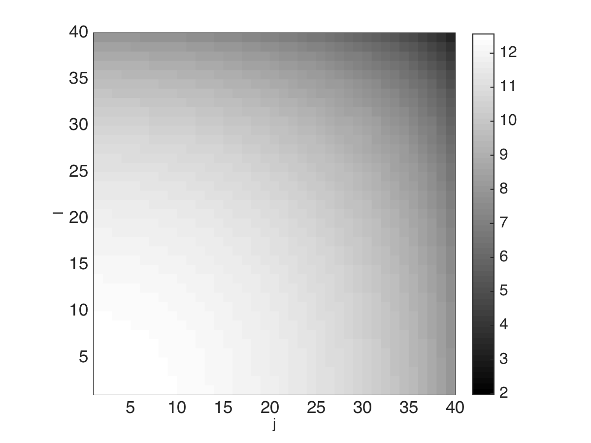
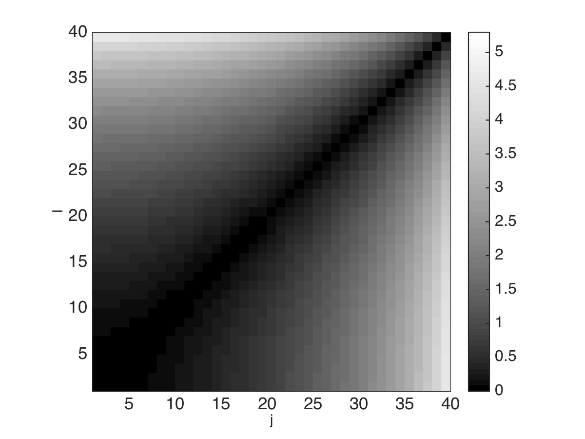
Fig. 2: Plot of the matrix with entries $\beta_{j}+\beta_{l}$ on the left and $|\beta_{j}-\beta_{l}|$ on the right, v.s. $j,l=1,\ldots,\mathcal{N}$, for the case of $\mathcal{N}=40$ propagating modes. The scaled wavenumber is $k=2\pi$ and the waveguide width is $D=20.25$. Note that the entries in the left plot are larger than $2\beta_{\mathcal{N}}=1.97$, whereas the entries near the diagonal in the right plot are small.

Note that there is mode coupling in this approximation, but only between the forward going mode amplitudes. This is due to the fact that $|\beta_{j}(\omega,z)-\beta_{l}(\omega,z)|$ is small at least for nearby indexes $j,l$, as illustrated in Figure 2. The power spectral density evaluated at such differences is not negligible, and the net coupling effect is described in the next section.

4.3 The coupled mode diffusion process

The $\varepsilon\to 0$ limit of the forward going mode amplitudes is stated in the next theorem. We derive it using Theorem 2 for the vector ${\itbf X}^{\varepsilon}\in\mathbb{R}^{2\mathcal{N}}$ obtained by concatenating the moduli and arguments of $b_{j}^{\varepsilon}$, with $j=1,\ldots,\mathcal{N}$. The differential equations for ${\itbf X}^{\varepsilon}$ follow from the system

$$\partial_{z}{\itbf b}^{\varepsilon}(\omega,z)\approx\bm{\Upsilon}^{\varepsilon(bb)}(\omega,z){\itbf b}^{\varepsilon}(\omega,z)\,,\quad z<z_{-}^{(t-1)},$$ (100)

with given ${\itbf b}^{\varepsilon}(\omega,z_{-}^{(t-1)})$. As explained in the previous section, the approximation in (100) means that there is an error that vanishes in the limit $\varepsilon\to 0$.

Theorem 1.

The complex mode amplitudes $\{{b}_{j}^{\varepsilon}(\omega,z)\}_{j=1}^{\mathcal{N}}$ converge in distribution as $\varepsilon\rightarrow 0$ to an inhomogeneous diffusion Markov process $\{{b}_{j}(\omega,z)\}_{j=1}^{{\cal N}}$ with generator $-{\cal L}_{z}^{{\cal N}}$ given below.

Let us write the limit process as

$${b}_{j}(\omega,z)=P_{j}^{1/2}(\omega,z)e^{i\psi_{j}(\omega,z)},\quad j=1,\ldots,{\cal N},$$

in terms of the power $P_{j}=|b_{j}|^{2}$ and the phase $\psi_{j}=\mbox{arg}\,b_{j}$. Then, we can express the infinitesimal generator of the limit diffusion as the sum of two operators

$${\cal L}_{z}^{{\cal N}}={\cal L}_{P,z}^{{\cal N}}+{\cal L}_{\psi,z}^{{\cal N}}.$$ (101)

The first is a partial differential operator in the powers

$${\cal L}_{P,z}^{{\cal N}}=\sum_{{\scriptsize\begin{array}[]{c}j,l=1\\ j\neq l\end{array}}}^{{\cal N}}G_{jl}^{(c)}(\omega,z)\left[P_{l}P_{j}\left(\frac{\partial}{\partial P_{j}}-\frac{\partial}{\partial P_{l}}\right)\frac{\partial}{\partial P_{j}}+(P_{l}-P_{j})\frac{\partial}{\partial P_{j}}\right]\,,$$ (102)

with symmetric matrix ${\bf G}^{(c)}(\omega,z)=\big{(}G^{(c)}_{jl}(\omega,z)\big{)}_{j,l=1}^{{\cal N}}$ of coefficients that are non-negative off the diagonal

$$G_{jl}^{(c)}(\omega,z)=\frac{\sigma^{2}\mu_{j}^{2}(z)\mu_{l}^{2}(z)}{4\beta_{j}(\omega,z)\beta_{l}(\omega,z)}\widehat{\mathcal{R}}[\beta_{j}(\omega,z)-\beta_{l}(\omega,z)]\,,\quad j\neq l\,,$$ (103)

and sum to zero in the rows

$$G_{jj}^{(c)}(\omega,z)=-\sum_{l=1,l\neq j}^{{\cal N}}G_{jl}^{(c)}(\omega,z)\,.$$ (104)

The second partial differential operator in (101) is with respect to the phases

$${\cal L}_{\psi,z}^{{\cal N}} =\frac{1}{8}\sum_{{\scriptsize\begin{array}[]{c}j,l=1\\ j\neq l\end{array}}}^{{\cal N}}G_{jl}^{(c)}(\omega,z)\left[\frac{P_{j}}{P_{l}}\frac{\partial^{2}}{\partial\psi_{l}^{2}}+\frac{P_{l}}{P_{j}}\frac{\partial^{2}}{\partial\psi_{j}^{2}}+2\frac{\partial^{2}}{\partial\psi_{j}\partial\psi_{l}}\right]+\frac{1}{2}\sum_{j,l=1}^{{\cal N}}G_{jl}^{(0)}(\omega,z)\frac{\partial^{2}}{\partial\psi_{j}\partial\psi_{l}}$$ (107)

$$+\frac{1}{2}\sum_{{\scriptsize\begin{array}[]{c}j,l=1\\ j\neq l\end{array}}}^{{\cal N}}G_{jl}^{(s)}(\omega,z)\frac{\partial}{\partial\psi_{j}}+\sum_{j=1}^{{\cal N}}\kappa_{j}^{{\cal N}}(\omega,z)\frac{\partial}{\partial\psi_{j}}\,,$$ (110)

with coefficients

$$G_{jl}^{(0)}(\omega,z)=\frac{\sigma^{2}\mu_{j}^{2}(z)\mu_{l}^{2}(z)}{4\beta_{j}(\omega,z)\beta_{l}(\omega,z)}\widehat{\mathcal{R}}(0)\,,\quad j,l=1,\ldots,\mathcal{N},$$ (111)

and

$$G_{jl}^{(s)}(\omega,z)=\frac{\sigma^{2}\mu_{j}^{2}(z)\mu_{l}^{2}(z)}{2\beta_{j}(\omega,z)\beta_{l}(\omega,z)}\int_{0}^{\infty}d\zeta\,\mathcal{R}(\zeta)\sin\left[(\beta_{j}(\omega,z)-\beta_{l}(\omega,z))\zeta\right]\,,\quad$$ (112)

for $j,l=1,\ldots,\mathcal{N}$ and $j\neq l$. The coefficient $\kappa_{j}^{{\cal N}}$ in the last term of (110) is

$$\kappa_{j}^{{\cal N}}(\omega,z)=\frac{\sigma^{2}}{2\beta_{j}(\omega,z)}\Big{\{}\Big{(}\frac{\pi^{2}j^{2}}{12}+\frac{1}{16}\Big{)}\mathcal{R}^{\prime\prime}(0)-\frac{3\mu_{j}^{2}(z)}{4}\mathcal{R}(0)\Big{\}}$$

$$-\sum_{{\scriptsize\begin{array}[]{c}l=1\\ j\neq l\end{array}}}^{{\cal N}}\frac{\mu_{j}^{2}(z)\mu_{l}^{2}(z)}{4\beta_{j}(\omega,z)\beta_{l}(\omega,z)[\beta_{j}(\omega,z)-\beta_{l}(\omega,z)]}\Big{[}\mathcal{R}(0)+\frac{\mathcal{R}^{\prime\prime}(0)}{[\beta_{j}(\omega,z)+\beta_{l}(\omega,z)]^{2}}\Big{]}$$ (115)

$$+\sum_{l>{\cal N}}\,\frac{\sigma^{2}\mu_{j}^{2}(z)\mu_{l}^{2}(z)}{2\beta_{j}\beta_{l}[\beta_{j}^{2}(\omega,z)+\beta_{l}^{2}(\omega,z)]^{2}}\Big{\{}-\beta_{l}(\omega,z)\mathcal{R}^{\prime\prime}(0)+\int_{0}^{\infty}d\zeta\,\mathcal{R}^{\prime\prime}(\zeta)e^{-\beta_{l}(\omega,z)\zeta}$$

$$\times\Big{[}[\beta_{l}^{2}(\omega,z)-\beta_{j}^{2}(\omega,z)]\cos(\beta_{j}(\omega,z)\zeta)-2\beta_{j}(\omega,z)\beta_{l}(\omega,z)\sin(\beta_{j}(\omega,z)\zeta)\Big{]}\Big{\}}.$$ (116)

Note that the coefficients of the partial derivatives with respect to the mode powers $P_{j}$ are independent of the phases $\psi_{j}$. This means that $\{|b_{j}^{\varepsilon}(\omega,z)|^{2}\}_{j=1}^{\mathcal{N}}$ converge in distribution in the limit $\varepsilon\to 0$ to the inhomogeneous diffusion Markov process $\{P_{j}(\omega,z)\}_{j=1}^{\mathcal{N}}$ with infinitesimal generator $-\mathcal{L}_{P,z}^{\mathcal{N}}$ defined in (102). The total power of the propagating modes satisfies

$$\mathcal{L}_{P,z}^{\mathcal{N}}\Big{[}\sum_{j=1}^{\mathcal{N}}P_{j}(\omega,z)\Big{]}=\sum_{{\scriptsize\begin{array}[]{c}j,l=1\\ j\neq l\end{array}}}^{{\cal N}}G_{jl}^{(c)}(\omega,z)\Big{[}P_{l}(\omega,z)-P_{j}(\omega,z)\Big{]}=0,$$ (117)

where we used (104) and the symmetry of matrix ${\bf G}^{(c)}(\omega,z)$. This implies that the total power is conserved

$$\sum_{j=1}^{\mathcal{N}}P_{j}(\omega,z)=\mbox{constant},\qquad z\in\big{(}z_{-}^{(t)},z_{-}^{(t-1)}\big{)}.$$ (118)

The evanescent waves do not contribute to the expression of the infinitesimal generator $\mathcal{L}_{P,z}^{\mathcal{N}}$, so they do not exchange energy with the propagating modes in the limit $\varepsilon\to 0$. However, they appear in the last coefficient (116) of the operator $\mathcal{L}_{\psi,z}^{\mathcal{N}}$, so they affect the phases of the mode amplitudes.

The limit Markov process $\{b_{j}(\omega,z)\}_{j=1}^{\mathcal{N}}$ is inhomogeneous due to the slow variations of the waveguide which make the coefficients of the operators (102) and (110) $z$ dependent. The slow variations also change the number of propagating modes at the turning points, and this leads to partial reflection of power, as described in the next section.

5 Transport and reflection of power in the waveguide

We now use the infinitesimal generator (101) to quantify the cumulative scattering effects in the waveguide. We begin in section 5.1 with the modes transmitted through the left part of the waveguide. The right going modes are discussed in 5.4. They are defined by the direct excitation from the source and the reflection at the turning points. We end with some numerical illustrations in section 5.7.

5.1 The left going waves

The wave propagation from the source at $z=0$ to the end $z=-Z_{M}$ of the support of variations of the waveguide can be described in the limit $\varepsilon\to 0$ as follows:

The left going mode amplitudes start with the values

$$b_{j}(\omega,0-)=b_{j,o}(\omega)=-\frac{f(\omega)y_{j}(\rho_{\star},0)}{2i\sqrt{\beta_{j}(\omega,0)}},\qquad j=1,\ldots,N^{(0)},$$ (119)

obtained from equation (83) and the observation that at $z>0$, where the opening $D(z)$ increases, the waves are right going.

In the sector $\big{(}z_{-}^{(1)},0\big{)}$ the amplitudes $\{{b}_{j}(\omega,z)\}_{j=1}^{N^{(0)}}$ evolve according to the diffusion Markovian dynamics with generator $-{\cal L}_{z}^{N^{(0)}}$, starting from $\{{b}_{j,o}(\omega)\}_{j=1}^{N^{(0)}}$. The first $N^{(0)}-1$ left going modes pass through the turning point

$$b_{j}(\omega,z_{-}^{(1)}-)=b_{j}(\omega,z_{-}^{(1)}+),\qquad j=1,\ldots,N^{(0)}-1,$$ (120)

but the last mode is reflected back.

In the sector $\big{(}z_{-}^{(2)},z_{-}^{(1)}\big{)}$ there are $N_{-}^{(1)}=N^{(0)}-1$ left going modes, with amplitudes evolving according to the diffusion Markovian dynamics with generator $-{\cal L}_{z}^{N_{-}^{(1)}}$, starting from the values (120) at $z=z_{-}^{(1)}-$. At the next turning point $z_{-}^{(2)}$, only the first $N_{-}^{(1)}-1$ modes pass through

$$b_{j}(\omega,z_{-}^{(2)}-)=b_{j}(\omega,z_{-}^{(2)}+),\qquad j=1,\ldots,N_{-}^{(1)}-1,$$ (121)

and the last mode is reflected back.

We continue this way until we reach $z=-Z_{M}$, with amplitudes $\{b_{j}(\omega,-Z_{M})\}_{j=1}^{N_{\rm min}}$ obtained from the diffusion Markovian dynamics with generator $-{\cal L}_{z}^{N_{\rm min}}$ over the interval $(-Z_{M},z_{-}^{(t_{M}^{-})})$, starting with the values $\{b_{j}(\omega,z_{-}^{(t_{M}^{-})}-)\}_{j=1}^{N_{\rm min}}$ determined as explained above, from the previous waveguide sectors.

The waveguide has no variations at $z<Z_{-M}$, so the left going mode amplitudes remain equal to their values at $-Z_{M}$, as stated in equation (86). The emerging wave is obtained from (29) and (49),

$$p^{\varepsilon}(\omega,\rho,z)\approx-\sum_{j=1}^{N_{\rm min}}\frac{y_{j}(\rho,-Z_{M})b_{j}(\omega,-Z_{M})}{\sqrt{\beta_{j}(\omega,-Z_{M})}}\exp\Big{[}-\frac{i}{\varepsilon}\int_{0}^{-Z_{M}}dz^{\prime}\beta_{j}(\omega,z^{\prime})$$

$$-\frac{i}{\varepsilon}\beta_{j}(\omega,-Z_{M})(z+Z_{M})\Big{]},\quad\mbox{for}~{}z<-Z_{M}.$$ (122)

5.2 The mean transmitted wave field

With the infinitesimal generator (101) and Kolmogorov’s equation, we now calculate the mean mode amplitudes

$$\big{<}b_{j}(\omega,z)\big{>}=\mathbb{E}\big{[}b_{j}(\omega,z)\big{]}.$$ (123)

In the first sector $(z_{-}^{(1)},0)$, these satisfy the evolution equations

$$\partial_{z}\big{<}b_{j}(\omega,z)\big{>}=-\Big{[}G_{jj}^{(c)}(\omega,z)-G_{jj}^{(0)}(\omega,z)+iG_{jj}^{(s)}(\omega,z)+2i\kappa_{j}^{N^{(0)}}(\omega,z)\Big{]}\frac{\big{<}b_{j}(\omega,z)\big{>}}{2},$$ (124)

solved backward in $z$, for $z\in\big{(}z_{-}^{(1)},0\big{)}$, starting from the values

$$\big{<}b_{j}(\omega,0-)\big{>}=b_{j,o}(\omega),\quad j=1,\ldots,N^{(0)}.$$ (125)

The coefficients in (124) are defined by (104), (111), (116) and

$$G_{jj}^{(s)}(\omega,z)=-\sum_{l=1,l\neq j}^{N^{(0)}}G_{lj}^{(s)}(\omega,z),$$ (126)

with $G_{lj}^{(s)}(\omega,z)$ given in (112). Because $-G_{jj}^{(c)}(\omega,z)+G_{jj}^{(0)}(\omega,z)>0$ (by Wiener-Khintchine theorem), we conclude from (134) that the mean mode amplitudes decay with $|z|$, and therefore

$$\left|\big{<}b_{j}(\omega,z_{-}^{(1)})\big{>}\right|<\big{|}b_{j,o}(\omega)\big{|},\qquad 1\leq j\leq N^{(0)}.$$ (127)

This decay models the randomization of the left going modes, and occurs on a $j$ dependent length scale, as illustrated in section 5.7. Similar to the case of waveguides with random perturbations of straight boundaries [5, Section 5], the modes with larger index $j$ randomize faster. Intuitively, this is because these modes propagate slowly along $z$, at group velocity $1/\partial_{\omega}\beta_{j}(\omega,z)$ that is small with respect to the wave speed, and bounce more often at the random boundary.

A similar calculation applies to the other sectors $\big{(}z_{-}^{(t)},z_{-}^{(t-1)}\big{)}$ of the waveguide, indexed by $t=1,\ldots t_{M}^{-}$. The only difference is that the starting values of the mode amplitudes are random, so we use conditional expectations

$$\big{<}b_{j}(\omega,z)\big{>}=\mathbb{E}\left[\mathbb{E}\left[b_{j}(\omega,z)\big{|}{\cal F}_{z_{-}^{(t-1)}}\right]\right],\qquad z<z_{-}^{(t-1)},$$ (128)

where $\mathcal{F}_{z_{-}^{(t-1)}}$ denotes the $\sigma$-algebra ( information) generated by the Markov limit process $\left\{b_{q}(\omega,z)\right\}_{q=1}^{N_{-}^{(t-1)}}$ at $z=z_{-}^{(t-1)}$. We obtain that $\big{<}b_{j}(\omega,z)\big{>}$ satisfies an equation like (124), with redefined coefficients for the $N_{-}^{(t-1)}$ number of propagating modes, and starting value $\big{<}b_{j}(\omega,z_{-}^{(t-1)})\big{>}$ calculated in the previous waveguide sector.

Proceeding this way we reach $z=-Z_{M}$. The mean transmitted wave is the expectation of (122), with $\big{<}b_{j}(\omega,-Z_{M})\big{>}$ obtained by solving equations (124) for all the sectors of the waveguide. The scattering effects at the random boundary add up in each sector, and the mean mode amplitudes decay, as explained above,

$$\left|\big{<}b_{j}(\omega,-Z_{M})\big{>}\right|<\left|\big{<}b_{j}(\omega,-z_{-}^{(t_{M}^{-})}\big{>}\right|<\ldots<\big{|}b_{j,o}(\omega)\big{|},\qquad 1\leq j\leq N_{\rm min}.$$ (129)

5.3 The transmitted power

Using the infinitesimal generator (102) of the Markov process $\{P_{j}(\omega,z)\}$, the $\varepsilon\to 0$ limit of the left going mode powers, we now calculate the mean and standard deviation of the transmitted power at $z<0$.

We proceed as in the previous section, one sector of the waveguide at a time, starting from the source. In the first sector $z\in\big{(}z_{-}^{(1)},0\big{)}$, the mean powers

$$\big{<}P_{j}(\omega,z)\big{>}=\mathbb{E}\left[P_{j}(\omega,z)\right],\qquad j=1,\ldots,N^{(0)},$$ (130)

evolve from the initial values $\big{<}P_{j}(\omega,0-)\big{>}=|b_{j,o}(\omega)|^{2}$ according to equation

$$\partial_{z}\begin{pmatrix}\big{<}P_{1}(\omega,z)\big{>}\\ \vdots\\ \big{<}P_{N^{(0)}}(\omega,z)\big{>}\end{pmatrix}=-{\bf G}^{(c)}(\omega,z)\begin{pmatrix}\big{<}P_{1}(\omega,z)\big{>}\\ \vdots\\ \big{<}P_{N^{(0)}}(\omega,z)\big{>}\end{pmatrix},$$ (131)

with matrix ${\bf G}^{(c)}(\omega,z)$ defined in (103)-(104), for $\mathcal{N}=N^{(0)}$.

In the next sectors $(z_{-}^{(t)},z_{-}^{(t-1)})$ we use conditional expectations

$$\big{<}P_{j}(\omega,z)\big{>}=\mathbb{E}\left[\mathbb{E}\left[P_{j}(\omega,z)\big{|}{\cal F}_{z_{-}^{(t-1)}}\right]\right],\qquad z<z_{-}^{(t-1)},$$ (132)

and obtain that the mean powers satisfy an equation like (131), with $N_{-}^{(t-1)}$ unknowns and $N_{-}^{(t-1)}\times N_{-}^{(t-1)}$ matrix ${\bf G}^{(c)}(\omega,z)$. These equations are solved backward in $z$, starting from the values $\big{<}P_{j}(\omega,z_{-}^{(t-1)})\big{>}$ computed in the previous sectors. Proceeding this way, we reach $z=-Z_{M}$, and obtain $\big{<}P_{j}(\omega,-Z_{M})\big{>}$, for $j=1,\ldots,N_{\rm min}.$

Note that unlike the expectations (123), the mean powers are coupled by the matrix ${\bf G}^{(c)}(\omega,z)$. This coupling models the exchange of power between the left going modes, induced by cumulative scattering at the random boundary of the waveguide. The exchange depends on the mode index, as illustrated in section 5.7. Specifically, the higher indexed modes transfer power more quickly than the others.

How much power is exchanged depends on the length of the sectors $\big{(}z_{-}^{(t)},z_{-}^{(t-1)}\big{)}$ of the waveguide. In short sectors, the exchange is mostly among the higher indexed modes. The longer the sectors, the more modes participate in the exchange and the power may become evenly distributed among the modes, independent of the starting value at $z_{-}^{(t-1)}$. This equipartition of energy has been explained in waveguides with straight walls in [18, Section 20.3], for a matrix ${\bf G}^{(c)}$ with non-zero off diagonal entries. By the Perron-Frobenius theorem, and due to energy conservation, such a matrix has a simple eigenvalue equal to zero, and the other eigenvalues are negative. It is straightforward to see from equation (131) that the solution converges at large $|z|$ to a vector in the null space of ${\bf G}^{(c)}$. Equation (104) gives that this space is spanned by the vector of all ones, so the power becomes evenly distributed at distances that exceed the equipartition distance. This length scale is defined by the inverse of the absolute value of the largest, non-zero eigenvalue of ${\bf G}^{(c)}$.

By the energy conservation (118), the transmitted power in the first sector of the waveguide is

$$\mathcal{P}_{\rm trans}(\omega,z)=\sum_{j=1}^{N^{(0)}}P_{j}(\omega,z)=\sum_{j=1}^{N^{(0)}}|b_{j,o}(\omega)|^{2},\qquad z\in(z_{-}^{(1)},0),$$ (133)

where the right hand side is the deterministic, total left going power emitted by the source. At the turning point $z_{-}^{(1)}$ the $N^{(0)}$-th mode is reflected back. The transmitted power to the next sector of the waveguide, carried by the remaining $N_{-}^{(1)}=N^{(0)}-1$ modes, is random and given by

$$\mathcal{P}_{\rm trans}(\omega,z)=\sum_{j=1}^{N_{-}^{(1)}}P_{j}(\omega,z)=\sum_{j=1}^{N_{-}^{(1)}}P_{j}(\omega,z_{-}^{(1)}),\qquad z\in(z_{-}^{(2)},z_{-}^{(1)}).$$ (134)

This repeats for the other sectors, and beyond $z=-Z_{M}$ we have

$$\mathcal{P}_{\rm trans}(\omega,z)=\sum_{j=1}^{N_{\rm min}}P_{j}(\omega,-Z_{M}),\qquad z\leq-Z_{M}.$$ (135)

In summary, the transmitted power is a piecewise constant function with jumps at the turning points, and random values determined by the sum of the mode powers entering each sector of the waveguide. Its mean is obtained by taking expectations in (133)-(135), and using the mean mode powers calculated as explained above.

The random fluctuations of $\mathcal{P}_{\rm trans}(\omega,z)$ about the mean are quantified by its standard deviation

$$\mbox{StD}\left[\mathcal{P}_{\rm trans}(\omega,z)\right]=\Big{\{}\sum_{j,l=1}^{N_{-}^{(t-1)}}\left[\big{<}\mathcal{P}_{jl}(\omega,z)\big{>}-\big{<}P_{j}(\omega,z)\big{>}\big{<}P_{l}(\omega,z)\big{>}\right]\Big{\}}^{1/2}$$ (136)

for $z\in(z_{-}^{(t)},z_{-}^{(t-1)})$ and $1\leq t\leq t_{M}^{-}$. To calculate it we need the second moments

$$\big{<}\mathcal{P}_{jl}(\omega,z)\big{>}=\mathbb{E}\left[{P}_{j}(\omega,z){P}_{l}(\omega,z)\right].$$ (137)

Again, these are obtained in one sector of the waveguide at a time, starting from the source, where

$$\big{<}\mathcal{P}_{jl}(\omega,0)\big{>}=|b_{j,o}(\omega)|^{2}|b_{l,o}(\omega)|^{2},\qquad j,l=1,\ldots,N^{(0)}.$$ (138)

The evolution equations of the moments (137) at $z\in\big{(}z_{-}^{(t)},z_{-}^{(t-1)}\big{)}$ are

$$\partial_{z}\big{<}\mathcal{P}_{jj}(\omega,z)\big{>}=2G_{jj}^{(c)}(\omega,z)\big{<}\mathcal{P}_{jj}(\omega,z)\big{>}-4\sum_{l=1}^{N_{-}^{(t-1)}}G_{jl}^{(c)}(\omega,z)\big{<}\mathcal{P}_{lj}(\omega,z)\big{>},$$ (139)

and

$$\partial_{z}\big{<}\mathcal{P}_{jq}(\omega,z)\big{>}=2G_{jq}^{(c)}(\omega,z)\big{<}\mathcal{P}_{jq}(\omega,z)\big{>}-\sum_{l=1}^{N_{-}^{(t-1)}}\Big{[}G_{jl}^{(c)}(\omega,z)\big{<}\mathcal{P}_{lq}(\omega,z)\big{>}$$

$$+G_{lq}^{(c)}(\omega,z)\big{<}\mathcal{P}_{jl}(\omega,z)\big{>}\Big{]},$$ (140)

for $j,q=1,\ldots,N_{-}^{(t-1)}$ and $j\neq q$. These equations are solved backward in $z$, with the starting values $\big{<}\mathcal{P}_{jq}(\omega,z_{-}^{(t-1)})\big{>}$ calculated from the previous sector.

5.4 The right going waves

Even though we consider the forward scattering approximation in each sector of the waveguide, there are both left and right going modes at $z<0$, due to reflection at the turning points. At $z>0$ we also have the right going waves emitted from the source. The analysis of the reflected mode amplitudes is more complicated, because they quantify cumulative scattering in the waveguide sectors traversed both ways: to the left by the incoming wave and to the right by the reflected wave.

In each sector $\big{(}z_{-}^{(t)},z_{-}^{(t-1)}\big{)}$ we obtain from (97) that the right going mode amplitudes satisfy

$${\itbf a}^{\varepsilon}(\omega,z)\approx\overline{{\bf P}^{\varepsilon(bb)}}(\omega,z;z_{-}^{(t-1)}){\itbf a}^{\varepsilon}(\omega,z_{-}^{(t-1)}),\qquad t=1,\ldots,t_{M}^{-}.$$ (141)

This looks similar to equation (98) that describes the evolution of the left going waves, but we have different boundary conditions, as we now explain.

Starting from the leftmost turning point $z_{-}^{(t_{M}^{-})}$, and denoting $\mathcal{N}=N_{-}^{(t_{M}^{-}-1)}$, we obtain from (85) the initial condition

$$a_{j}^{\varepsilon}\big{(}\omega,z_{-}^{(t_{M}^{-})}\big{)}={\rm R}_{\mathcal{N}}^{\varepsilon}\big{(}\omega,z_{-}^{(t_{M}^{-})}\big{)}b_{\mathcal{N}}^{\varepsilon}\big{(}\omega,z_{-}^{(t_{M}^{-})}\big{)}\delta_{j\mathcal{N}},\qquad j=1,\ldots,\mathcal{N},$$ (142)

for the vector ${\itbf a}^{\varepsilon}(\omega,z)\in\mathbb{C}^{\mathcal{N}}$, where $\delta_{j\mathcal{N}}$ is the Kronecker delta symbol and ${\rm R}_{\mathcal{N}}^{\varepsilon}$ is reflection coefficient defined in (82). The amplitudes of the right going modes impinging on the next turning point are obtained from (141)

$${\itbf a}^{\varepsilon}(\omega,z_{-}^{(t_{M}^{-}-1)}-)\approx\Big{[}{\bf P}^{\varepsilon(bb)}(\omega,z_{-}^{(t_{M}^{-})};z_{-}^{(t_{M}^{-}-1)})\Big{]}^{T}{\itbf a}^{\varepsilon}(\omega,z_{-}^{(t_{M}^{-})}),$$ (143)

using that the propagator ${\bf P}^{\varepsilon(bb)}$ is approximately unitary. This follows from the energy conservation relation (118), which holds in the limit $\varepsilon\to 0$, independent of the initial conditions.

On the right of the turning point $z_{-}^{(t_{M}^{-}-1)}$ there is an extra right going mode. Renaming $\mathcal{N}=N_{-}^{(t_{M}^{-}-2)}$, we obtain the following initial condition for the vector ${\itbf a}^{\varepsilon}(\omega,z)$: Its first $\mathcal{N}-1$ components are given in (143), and the last component is

$$a_{\mathcal{N}}^{\varepsilon}\big{(}\omega,z_{-}^{(t_{M}^{-}-1)}\big{)}={\rm R}_{\mathcal{N}}^{\varepsilon}\big{(}\omega,z_{-}^{(t_{M}^{-}-1)}\big{)}b_{\mathcal{N}}^{\varepsilon}\big{(}\omega,z_{-}^{(t_{M}^{-}-1)}\big{)}.$$ (144)

These amplitudes and the $\mathcal{N}\times\mathcal{N}$ propagator ${\bf P}^{\varepsilon(bb)}(\omega,z;z_{-}^{(t_{M}^{-}-2)})$ determine the amplitudes of the right going modes impinging on the turning point $z_{-}^{(t_{M}^{-}-2)}$ and so on.

Proceeding this way we obtain the amplitudes $\{a_{j}^{\varepsilon}(\omega,0-)\}_{j=1}^{N^{(0)}}$ on the left of the source. The amplitudes at $z=0+$ are given by these and the source conditions (83). The analysis of forward propagation at $z>0$ is similar to that in section 5.1, with the exception that at the turning points $z_{+}^{(t)}$, for $1\leq t\leq t_{M}^{+}$, there is no reflection. We add instead a new mode with zero initial condition, as stated in (88).

5.5 The net reflected power

The calculation of the statistical moments of the right going mode amplitudes in the limit $\varepsilon\to 0$ requires the infinitesimal generator of the limit propagator ${\bf P}^{\varepsilon(bb)}$, in each sector of the waveguide. This operator can be obtained using Theorem 2, but the calculation is complex. Here we quantify only the net reflected power at each turning point, without asking how this power gets distributed among the modes as they propagate toward the right.

The net reflected power is determined by the transmitted power in the left part of the waveguide, using energy conservation. Specifically, starting from the leftmost turning point, the net reflected power is

$$\mathcal{P}_{\rm refl}(\omega,z)=P_{N_{-}^{(t_{M}^{-}-1)}}(\omega,z_{-}^{(t_{M}^{-})}+),\qquad z\in\big{(}z_{-}^{(t_{M}^{-})},z_{-}^{(t_{M}^{-}-1)}\big{)},$$ (145)

where the right hand side is the power of the left going turning mode, analyzed in section 5.1. Here we used the conservation relation

$$\lim_{\varepsilon\to 0}\sum_{j=1}^{N_{-}^{(t_{M}^{-}-1)}}|a_{j}^{\varepsilon}(\omega,z)|^{2}=\mbox{constant},\quad\mbox{for}~{}z\in\big{(}z_{-}^{(t_{M}^{-})},z_{-}^{(t_{M}^{-}-1)}\big{)},$$

derived the same way as (118), equation (142) and $\lim_{\varepsilon\to 0}|{\rm R}_{\mathcal{N}}^{\varepsilon}|=1$.

At the next turning point $z_{-}^{(t_{M}^{-}-1)}$ we add a new mode amplitude, and the net reflected power increases to

$$\mathcal{P}_{\rm refl}(\omega,z)=P_{N_{-}^{(t_{M}^{-}-1)}}(\omega,z_{-}^{(t_{M}^{-})}+)+P_{N_{-}^{(t_{M}^{-}-2)}}(\omega,z_{-}^{(t_{M}^{-}-1)}+),$$ (146)

for $z\in\big{(}z_{-}^{(t_{M}^{-}-1)},z_{-}^{(t_{M}^{-}-2)}\big{)}$, and so on. Proceeding this way we obtain that the net reflected power is a piecewise constant function at $z<0$, with jumps at the turning points $z_{-}^{(t)}$ indexed by $1\leq t\leq t_{M}^{-}$. At the source location this equals

$$\mathcal{P}_{\rm refl}(\omega,0)=\sum_{t=1}^{t_{M}^{-}}P_{N_{-}^{(t-1)}}(\omega,z_{-}^{(t)}+),$$ (147)

and its mean and standard deviation are determined by those of the turning wave powers, calculated in section 5.1. By comparing with (133-135) we obtain the global conservation of energy relation

$$\mathcal{P}_{\rm refl}(\omega,0)+\mathcal{P}_{\rm trans}(\omega,-Z_{M})=\sum_{j=1}^{N^{(0)}}|b_{j,o}(\omega)|^{2}.$$ (148)

Therefore the first two moments of the net transmitted and reflected powers are related through:

$$\left<\mathcal{P}_{\rm refl}(\omega,0)\right> = \sum_{j=1}^{N^{(0)}}|b_{j,o}(\omega)|^{2}-\left<\mathcal{P}_{\rm trans}(\omega,-Z_{M})\right>,$$ (149)

$$\mbox{StD}\left[\mathcal{P}_{\rm refl}(\omega,0)\right] = \mbox{StD}\left[\mathcal{P}_{\rm trans}(\omega,-Z_{M})\right].$$ (150)

5.6 The net power transmitted to the right

There is no mode reflection at $z>0$, and the net transmitted power to the right is

$$\mathcal{P}_{\rm trans,right}(\omega,z)=\lim_{\varepsilon\to 0}\sum_{j=1}^{N^{(0)}}|a_{j}^{\varepsilon}(\omega,0+)|^{2},\qquad z>0,$$ (151)

where the equality means having the same statistical distribution, and

$$a_{j}^{\varepsilon}(\omega,0+)=a_{j}^{\varepsilon}(\omega,0-)+a_{j,o}(\omega),\qquad a_{j,o}(\omega)=\frac{\widehat{f}(\omega)y_{j}(\rho_{\star},0)}{2i\sqrt{\beta_{j}(\omega,0)}}.$$ (152)

The calculation of the statistical moments of (151) is as complicated as the calculation of the moments of the limit right going mode amplitudes. Specifically, it requires the infinitesimal generator of the $\varepsilon\to 0$ limit of the propagator ${\bf P}^{\varepsilon(bb)}$, in particular, we need to characterize the phases of the reflection coefficients ${\rm R}_{N_{-}^{(t-1)}}^{\varepsilon}\big{(}\omega,z_{-}^{(t)}\big{)}$, $t=1,\ldots,t_{M}^{-}$. By extrapolating the results given in [8] (in which the standard deviation of the fluctuations of the boundary was smaller), we could anticipate that these phases are independent and uniformly distributed over $[0,2\pi]$. We could then anticipate that the mean power transmitted to the right is

$$\left<\mathcal{P}_{\rm trans,right}(\omega,z)\right> = \left<\mathcal{P}_{\rm refl}(\omega,0)\right>+\sum_{j=1}^{N^{(0)}}|a_{j,o}(\omega)|^{2}$$ (153)

$$= \sum_{j=1}^{N^{(0)}}|a_{j,o}(\omega)|^{2}+\sum_{j=1}^{N^{(0)}}|b_{j,o}(\omega)|^{2}-\left<\mathcal{P}_{\rm trans}(\omega,-Z_{M})\right>,$$

for any $z>0$.

5.7 Numerical illustration

In this section we illustrate with some plots the exchange of power among the propagating modes in the left part $z<0$ of the waveguide, due to a point source at ${{\itbf x}}_{\star}=(D(0)/7,0)$. For comparison, we also consider other initial conditions, where the excitation at $z=0$ is for a single mode at a time.

We take a waveguide with a straight axis that has a single turning point, at arc length $z_{-}^{(1)}=-L=-1000\lambda$, where $\lambda$ is the wavelength. The waveguide opening $D(z/L)$ increases linearly in $z$ in the interval $[-L,0]$, from the value $20\lambda$ to $20.49\lambda$, and transitions as a cubic polynomial to the constant $19.999\lambda$ at $z<-L-0.2\lambda$ and $20.491\lambda$ at $z>0.2\lambda$. Thus, there are $N^{(0)}=40$ propagating modes at $z>-L$ and $N_{-}^{(1)}=39$ modes at $z<-L$. The top and bottom boundaries of the waveguide are straight and parallel at $z\in(-\infty,-L-0.2\lambda)\cup(0.2\lambda,\infty)$.

The auto-correlation function $\mathcal{R}$ of the process $\nu(\zeta)$ is a Gaussian with standard deviation $1$. The correlation length of the fluctuations is $\ell=3\lambda$, so $\varepsilon=\ell/L=0.003$, and the standard deviation $\sigma$ of the fluctuations equals $\sqrt{\varepsilon}$.

We can describe approximately what to expect in terms of the randomization of the mode amplitudes and the exchange of power among the modes by looking at the following length scales calculated in a waveguide with constant opening equal to $D(0)$:

1.The mode dependent scattering mean free path

$$L_{j,{\rm smf}}=\frac{2}{G_{jj}^{(0)}(\omega,0)-G_{jj}^{(c)}(\omega,0)},\qquad j=1,\ldots,40,$$ (154)

which is the scale of decay of the mean mode amplitudes, as seen from (124).

2. The mode dependent transport mean free paths,

$$L_{j,{\rm tmf}}=-\frac{2}{G_{jj}^{(c)}(\omega,0)},\qquad j=1,\ldots,40,$$ (155)

defined in terms of the diffusion coefficient $-G_{jj}^{(c)}$ of the mode power infinitesimal generator (102). The modes exchange power with their neighbors as they propagate at distances of order (155).

3. The equipartition distance $L_{\rm eq}$, which is defined as the inverse of the absolute value of the largest, non-zero eigenvalue of matrix ${\bf G}^{(c)}(\omega,0)$. At distances of order $L_{\rm eq}$, we expect that the power gets evenly distributed among the modes, independent of the excitation at $z=0$.

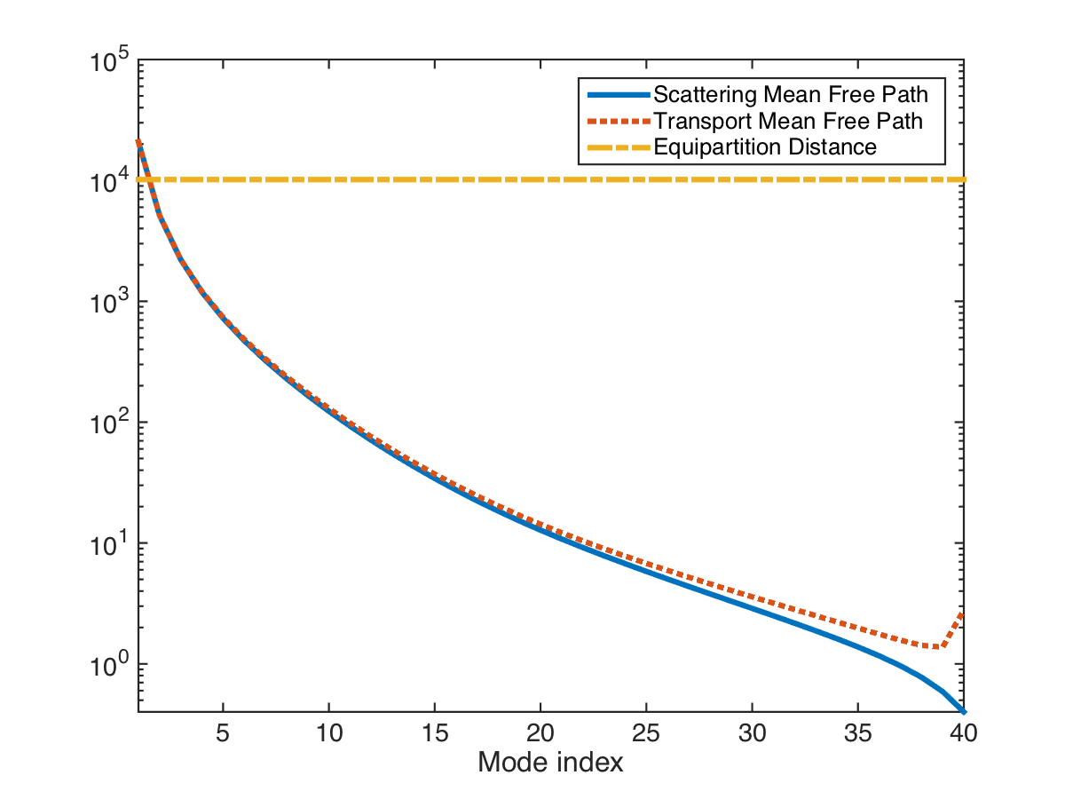
Fig. 3: The three length scales that quantify net scattering in a waveguide with constant opening $D(0)$. The solid blue line is for the scattering mean free path (154). The dashed red line is for the transport mean free path (155). The yellow dashed line is for the equipartition distance. The abscissa is the mode index $j=1,\ldots,40$ and the ordinate is in units of $\lambda$.

We display these scales in Figure 3 and observe that at the distance $L=1000\lambda$ between the source and the turning point, we have

$$L\geq L_{j,{\rm smf}},L_{j,{\rm tmf}},\qquad j=5,\ldots,40.$$

Thus, these modes should be randomized and moreover, they should share their power with the other modes. Because $L<L_{\rm eq}$, we expect that at least the first five modes have not shared all their power with the other modes.

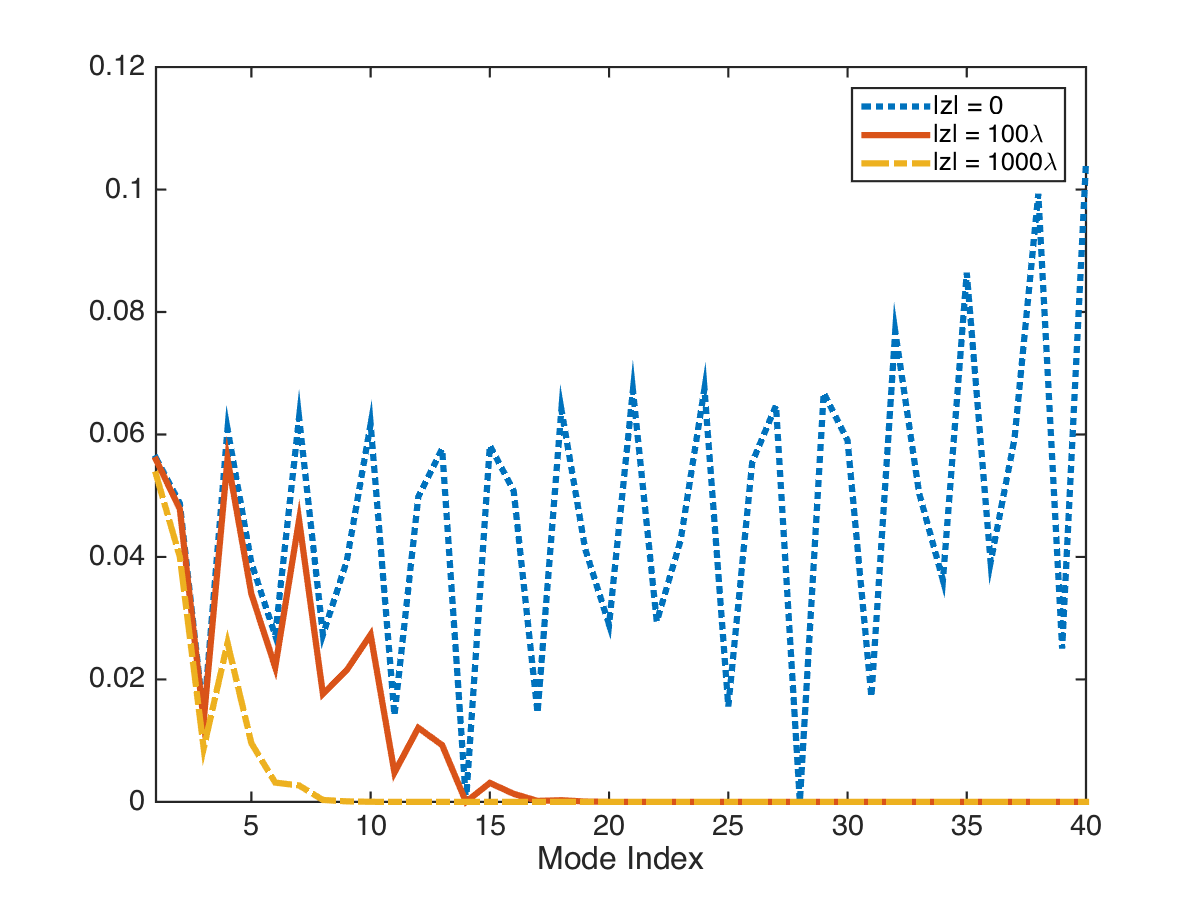
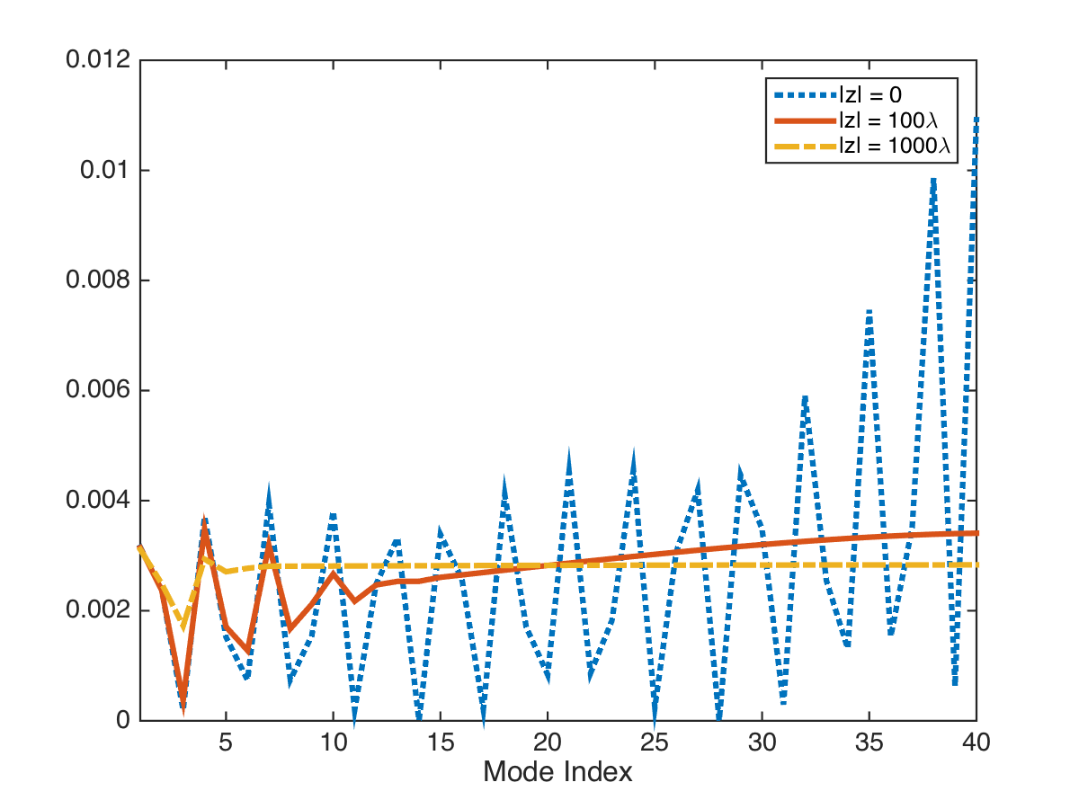
Fig. 4: Display of the absolute value of the mean mode amplitudes $|\big{<}b_{j}(\omega,z)\big{>}|$ (left) and the mean mode powers $\big{<}P_{j}(\omega,z)\big{>}$ v.s. the mode index $j$ at three different distances from the source: The blue dashed line corresponds to the initial values at $z=0$, due to a point source at location $(D(0)/7,0)$. The full red line is for $|z|=100\lambda$ and the yellow line is for $|z|=L=1000\lambda$. The abscissa is the mode index $j=1,\ldots,40$.

These expectations are confirmed by the results displayed in Figure 4, where we show the absolute values $|\big{<}b_{j}(\omega,z)\big{>}|$ of the mean mode amplitudes (left plot) and the mean mode powers $\big{<}P_{j}(\omega,z)\big{>}$ (right plot) at three distances from the point source. The dashed blue line is for $z=0$, so it corresponds to the initial values (119) of the mode amplitudes, which oscillate in $j$ due to the factor

$$y_{j}(\rho_{\star},0)=\sqrt{\frac{2}{D(0)}}\sin\Big{[}\Big{(}\frac{\rho_{\star}}{D(0)}+\frac{1}{2}\Big{)}\pi j\Big{]},\qquad j=1,\ldots,N^{(0)},~{}~{}\rho_{\star}=\frac{D(0)}{7}.$$

As we increase the distance $|z|$ from the source, the left plot in Figure 4 illustrates the decay of the mean mode amplitudes. We note that at $|z|=100\lambda$, the modes indexed by $j>15$ have negligible mean, and at the turning point $|z|=L=1000\lambda$, the modes indexed by $j>5$ have negligible mean. This is as expected from Figure 3, because because $L_{j,{\rm smf}}<100\lambda$ for $j>15$ and $L_{j,{\rm smf}}<1000\lambda$ for $j>5$. The right plot in Figure 4 illustrates the effect of exchange of power among the modes. The scattering mean free path and the transport mean free path are almost the same in this simulation, as shown in Figure 3, and we note that at the turning point $|z|=L=1000\lambda$ the modes indexed by $j>5$ have almost the same power.

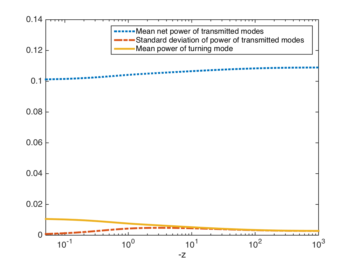
Fig. 5: Display of the mean net power of the transmitted modes in dashed blue line, of the standard deviation of this power in dashed red line, and the mean power of the turning mode, indexed by $j=40$. The abscissa is the arc length in units of $\lambda$ (in logarithmic scale).

In Figure 5 we display the mean and standard deviation of the net power $\sum_{j=1}^{39}P_{j}(\omega,z)$ of the modes that are transmitted through the turning point, and the mean power of the turning mode, as functions of $z$. At $|z|=L=1000\lambda$, these determine the transmitter power (134) beyond the turning point, and the reflected power (147). Note that in this case cumulative scattering at the random boundary is beneficial for power transmission through the waveguide. In the absence of the random fluctuations there would be no power exchange between the modes, and the transmitted power would equal $\sum_{j=1}^{39}P_{j}(\omega,0)$. As seen in Figure 4, the turning mode has the largest mode amplitude initially, and all its power would be reflected back. The cumulative scattering at the random boundary leads to rapid exchange of the power of the turning mode, as shown in the right plot of Figure 4, and much less power is reflected. The standard deviation of the net power of the first $39$ modes, shown with the red dashed line in Figure 5, is smaller than its mean. Thus, $\sum_{j=1}^{39}P_{j}(\omega,z)\approx\sum_{j=1}^{39}\big{<}P_{j}(\omega,z)\big{>},$ with less than $10\%$ relative error (i.e., random fluctuations).

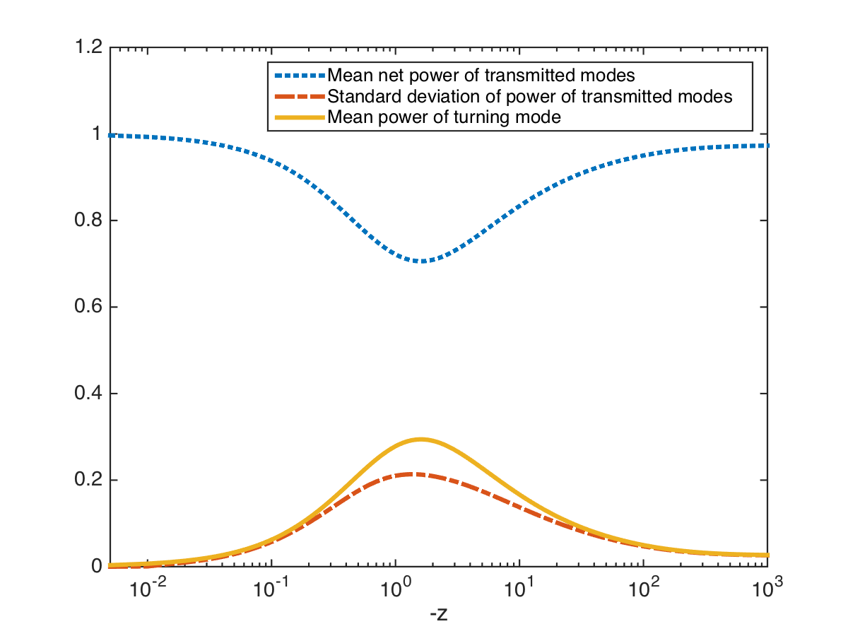
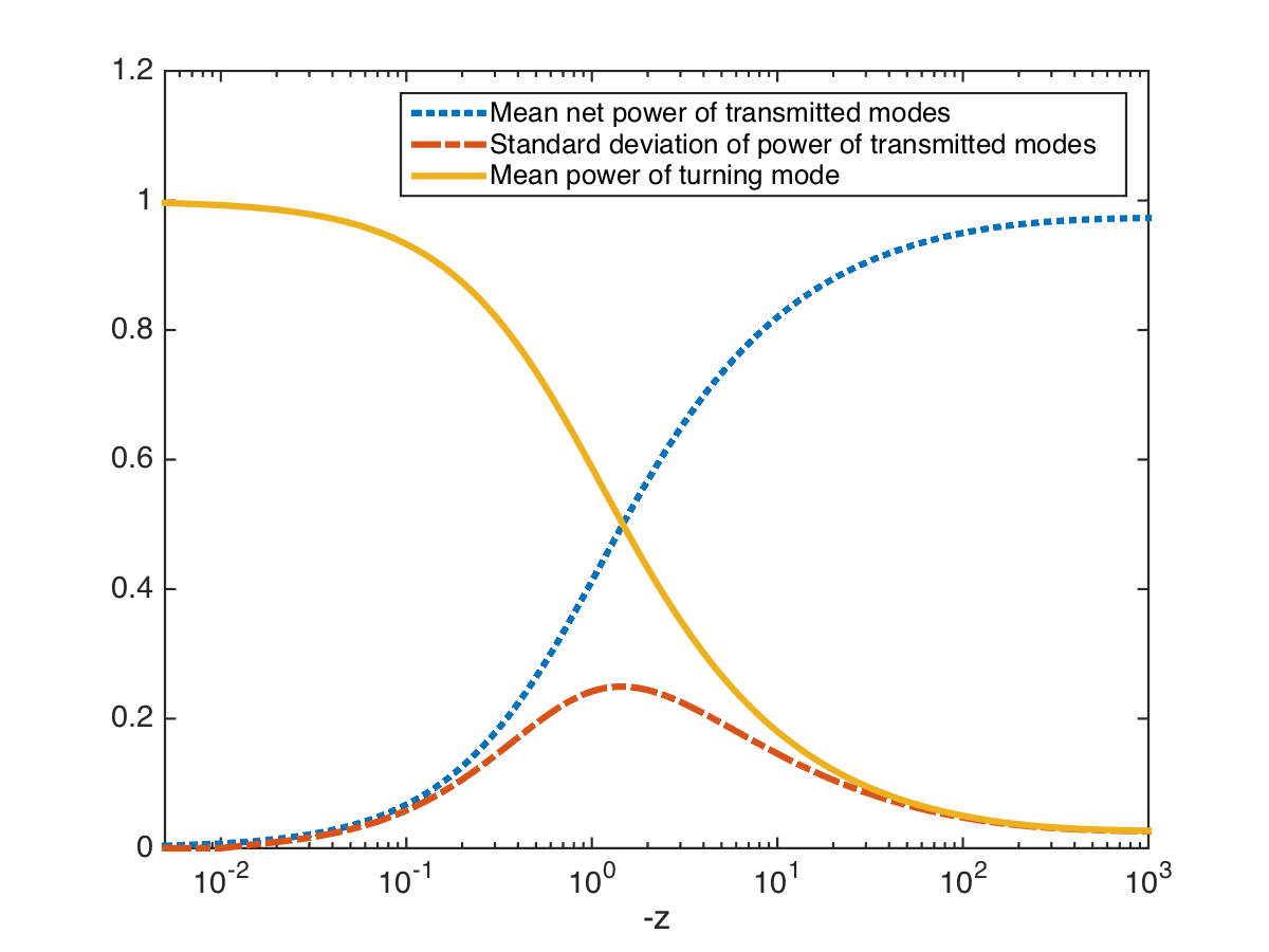
Fig. 6: Display of the mean net power of the transmitted modes in dashed blue line, of the standard deviation of this power in dashed red line, and the mean power of the turning mode, indexed by $j=40$. The abscissa is the arc length in units of $\lambda$ (in logarithmic scale). Only one mode was excited initially, the $39$-th one in the left plot and the $40$-th one in the right plot.

The last illustration, in Figure 6, shows the mean and standard deviation of $\sum_{j=1}^{39}P_{j}(\omega,z)$, and the mean power $\big{<}P_{40}(\omega,z)\big{>}$ of the turning mode, as functions of $z$, for initial excitations of a single mode. In the left plot the $39$-th mode is excited, and in the right plot the $40$-th mode is excited. In the absence of the random fluctuations, these initial conditions would determine the transmitted power at the turning point. Specifically, in the first case the power would stay in the $39$-th mode and would propagate through, whereas in the second case the power of the $40$-th mode would be totally reflected. The cumulative scattering in the random waveguide distributes the power among the modes, and we note in the left plot of Figure 6 that slightly less power is transmitted, due to the power transfer to the turning mode, whereas in the right plot, most of the power is transmitted, due to the transfer of power from the turning mode to the other modes.

5.8 Universal transmission properties for strong scattering

In case of strong scattering, the mean transmitted power through the left part of the waveguide becomes universal and equal to ${\cal P}_{0}N_{\rm min}/N^{(0)}$, where ${\cal P}_{0}=\sum_{j=1}^{N^{(0)}}|b_{j,o}(\omega)|^{2}$ is the power transmitted to the left by the source. More exactly, if scattering is so strong that equipartition is reached in each section between two turning points, in the sense that $z_{-}^{(t-1)}-z_{-}^{(t)}>L_{\rm eq}^{t}$ for all $t=1,\ldots,t_{M}^{-}$ (where $L_{\rm eq}^{t}$ is the equipartition distance in the section $(z_{-}^{(t)},z_{-}^{(t-1)})$), then the fraction of mean power transmitted through the $t$-th turning point $z_{-}^{(t)}$ is $1-1/N^{(t-1)}_{-}$, because the $N^{(t-1)}_{-}$-th mode carrying a fraction $1/N^{(t-1)}_{-}$ of the mean power is reflected. By denoting $\left<{\cal P}^{(t-1)}_{\rm trans}\right>$ the net transmitted power in the $t$-th section $(z_{-}^{(t)},z_{-}^{(t-1)})$, we get the recursive relation

$$\left<{\cal P}^{(t)}_{\rm trans}\right>=\left<{\cal P}^{(t-1)}_{\rm trans}\right>(N^{(t-1)}_{-}-1)/N^{(t-1)}_{-},\quad t=1,\ldots,t_{M}^{-},$$ (156)

which gives that the mean transmitted power at $-Z_{M}$ is ${\cal P}_{0}N_{\rm min}/N^{(0)}$.

6 Diffusion approximation theorem

In this section we state and prove the diffusion approximation theorem used to obtain the asymptotic limit of the mode amplitudes in section 4. We state the theorem for a general system of random differential equations

$$\frac{d{\bm{X}}^{\varepsilon}(z)}{dz}=\frac{1}{\sqrt{\varepsilon}}{\itbf F}\big{(}{\bm{X}}^{\varepsilon}(z),q^{\varepsilon}(z),{\bm{\theta}}^{\varepsilon}(z),z\big{)},\quad z>0,$$ (157)

with unknown vector ${\bm{X}}^{\varepsilon}\in\mathbb{R}^{d}$ satisfying the initial condition ${\bm{X}}^{\varepsilon}(0)={\itbf x}_{o}$, and right hand side defined by a function of the form

$${\itbf F}\big{(}{\bm{X}},q,{\bm{\theta}},z\big{)}=\sum_{j=1}^{p}{\itbf F}^{(j)}\big{(}{\bm{X}},q,\theta_{j},z\big{)},\quad\mbox{for}~{}~{}\bm{\theta}=\big{(}\theta_{j}\big{)}_{j=1}^{p}\in\mathbb{R}^{p}.$$ (158)

The second argument of ${\itbf F}$ is defined by $q^{\varepsilon}(z)=q(z/\varepsilon)$, where $q(z)$ is a stationary and ergodic Markov process taking values in a space $E$, with generator $Q$ and stationary distribution $\pi_{q}$. We assume that $Q$ satisfies the Fredholm alternative, which holds true for many different classes of Markov processes [18, section 6.3.3]. Note that the Markovian assumption on the driving process $q$ is convenient for the proof, but the statement of the diffusion approximation theorem 2 generalizes to a process $q$ that is not Markovian, but $\phi$-mixing with $\phi\in L^{1/2}$ [25, Sec. 4.6.2].

The third argument of ${\itbf F}$ is the vector valued function $\bm{\theta}^{\varepsilon}(z)$ taking values in $\mathbb{R}^{p}$, with components satisfying the equation

$$\frac{d\theta_{j}^{\varepsilon}}{dz}=\frac{1}{\varepsilon}\beta_{j}(z),\qquad j=1,\ldots,p,$$

where $\beta_{j}(z)$ is a $\mathbb{R}$-valued smooth function, bounded as $C\leq\beta_{j}(z)\leq 1/C$ for some constant $C>0$.

We assume that the components ${\itbf F}^{(j)}$ in (158) satisfy the following conditions, for all $j=1,\ldots,p$:

1. The mappings $({\itbf x},z)\in\mathbb{R}^{d}\times\mathbb{R}\to{\itbf F}^{(j)}({\itbf x},q,\theta_{j},z)\in\mathbb{R}^{d}$ are smooth for all $q\in E$ and $\theta_{j}\in\mathbb{R}$.

2. The mappings $q\in E\to{\itbf F}^{(j)}({\itbf x},q,\theta_{j},z)$ are centered with respect to the stationary distribution $\pi_{q}$,

   $$\mathbb{E}[{\itbf F}^{(j)}({\itbf x},q(0),\theta,z)]=\int_{E}{\itbf F}^{(j)}({\itbf x},q,\theta_{j},z)\pi_{q}(dq)=0,$$

   for any ${\itbf x}\in\mathbb{R}^{d}$, $\theta_{j}\in\mathbb{R}$ and $z\in\mathbb{R}$.

3. The mappings $\theta_{j}\in\mathbb{R}\to{\itbf F}^{(j)}({\itbf x},q,\theta_{j},z)$ are periodic with period $1$ for all ${\itbf x}\in\mathbb{R}^{d}$ and $q\in E$.

Theorem 2.

Let ${\bm{X}}^{\varepsilon}(z)$ be the solution of (157), with right hand side $\bm{F}$ defined in terms of the functions $\bm{F}^{(j)}$as in (158), and $\bm{F}^{(j)}$ satisfying the three properties above. In the limit $\varepsilon\to 0$, the continuous processes $({\bm{X}}^{\varepsilon}(z))_{z\geq 0}$ converge in distribution to the Markov diffusion process $({\bm{X}}(z))_{z\geq 0}$ with the inhomogeneous generator

$${\cal L}_{z}f({\itbf x}) =\sum_{m=1}^{d}{\textsl{h}}_{m}({\itbf x},z)\partial_{x_{m}}f({\itbf x})+\sum_{m,n=1}^{d}{\textsl{a}}_{m,n}({\itbf x},z)\partial_{x_{m}x_{n}}^{2}f({\itbf x}),$$ (159)

$${\textsl{h}}_{m}({\itbf x},z) =\sum_{n=1}^{d}\big{<}\int_{0}^{\infty}\mathbb{E}\left[{F}_{n}({\itbf x},q(0),\cdot,z)\partial_{x_{n}}{F}_{m}({\itbf x},q(\zeta),\cdot+{\bm{\beta}}(z)\zeta,z)\right]d\zeta\big{>}_{{\bm{\beta}}(z)},$$ (160)

$${\textsl{a}}_{m,n}({\itbf x},z) =\big{<}\int_{0}^{\infty}\mathbb{E}\left[{F}_{n}({\itbf x},q(0),\cdot,z){F}_{m}({\itbf x},q(\zeta),\cdot+{\bm{\beta}}(z)\zeta,z)\right]d\zeta\big{>}_{{\bm{\beta}}(z)},$$ (161)

where $\big{<}.\big{>}_{\bm{\beta}}$ is the mean value for almost periodic functions,

$$\big{<}{\itbf H}(\cdot)\big{>}_{\bm{\beta}}=\lim_{S\to\infty}\frac{1}{S}\int_{0}^{S}{\itbf H}({\bm{\theta}}+{\bm{\beta}}s)ds.$$

Note that the mean values for the terms involved in (160-161) exist and are independent of ${\bm{\theta}}$, since the functions

$$G_{n,m}(s) =\int_{0}^{\infty}\mathbb{E}\left[{F}_{n}({\itbf x},q(0),{\bm{\theta}}+{\bm{\beta}}s,z){F}_{m}({\itbf x},q(\zeta),{\bm{\theta}}+{\bm{\beta}}s+{\bm{\beta}}\zeta,z)\right]d\zeta,$$

$$\tilde{G}_{n,m}(s) =\int_{0}^{\infty}\mathbb{E}\left[{F}_{n}({\itbf x},q(0),{\bm{\theta}}+{\bm{\beta}}s,z)\partial_{x_{n}}{F}_{m}({\itbf x},q(\zeta),{\bm{\theta}}+{\bm{\beta}}s+{\bm{\beta}}\zeta,z)\right]d\zeta,$$

are periodic or almost periodic in $s$, for any fixed ${\itbf x}$ and $q$.

Proof. Let us define the projection on the torus $\mathbb{S}\simeq\mathbb{R}/\mathbb{Z}$:

$$\theta\in\mathbb{R}\to\dot{\theta}=\theta\mbox{ mod }1\in\mathbb{S},$$

and observe that if a function $f(\theta)$ is periodic with period $1$, then $f(\theta)=f(\dot{\theta})$. We also define $\dot{{\bm{\theta}}}^{\varepsilon}(z)={\bm{\theta}}^{\varepsilon}(z)$ mod $1$, and $Z(z)=z$. The process $({\bm{X}}^{\varepsilon}(z),q^{\varepsilon}(z),\dot{{\bm{\theta}}}^{\varepsilon}(z),Z(z))_{z\geq 0}$ is a Markov process with values in $\mathbb{R}^{d}\times E\times\mathbb{S}^{p}\times\mathbb{R}$ and infinitesimal generator

$${\cal L}^{\varepsilon}=\frac{1}{\varepsilon}\big{(}Q+{\bm{\beta}}(Z)\cdot\nabla_{\dot{{\bm{\theta}}}}\big{)}+\frac{1}{\sqrt{\varepsilon}}{\itbf F}({\bm{X}},q,\dot{{\bm{\theta}}},Z)\cdot\nabla_{\bm{X}}+{\partial_{Z}}\,.$$ (162)

One can show by the perturbed test function method [18, Section 6.3.2] and Lemma 4 that the continuous processes $({\bm{X}}^{\varepsilon}(z),Z(z))_{z\geq 0}$ converge in distribution to the Markov diffusion process $({\bm{X}}(z),Z(z))_{z\geq 0}$ with the homogeneous generator:

$${\cal L}f({\itbf x},Z)={\partial_{Z}}f({\itbf x},Z)$$ (163)

$$\hskip 3.61371pt+\big{<}\int_{0}^{\infty}\mathbb{E}\left[{\itbf F}({\itbf x},q(0),\cdot,Z)\cdot\nabla_{\itbf x}\left({\itbf F}({\itbf x},q(\zeta),\cdot+{\bm{\beta}}(Z)\zeta,Z)\cdot\nabla_{\itbf x}f({\itbf x},Z)\right)\right]d\zeta\big{>}_{{\bm{\beta}}(z)}.$$

Since $(Z(z))_{z\geq 0}$ is deterministic, we conclude that $({\bm{X}}(z))_{z\geq 0}$ is a Markov process and its inhomogeneous generator is

$${\cal L}_{z}f({\itbf x})=\big{<}\int_{0}^{\infty}\mathbb{E}\left[{\itbf F}({\itbf x},q(0),\cdot,z)\cdot\nabla_{\itbf x}\left({\itbf F}({\itbf x},q(\zeta),\cdot+{\bm{\beta}}(z)\zeta,z)\cdot\nabla_{\itbf x}f({\itbf x})\right)\right]d\zeta\big{>}_{{\bm{\beta}}(z)}$$ (164)

or equivalently (159). $\Box$

Lemma 3.

We have the following two statements:

1. Let $\beta\in\mathbb{R}\backslash\{0\}$. Let $g(q,\theta)$ be a bounded function, periodic in $\theta\in\mathbb{R}$ with period $1$, such that

$$\mathbb{E}[g(q(0),\theta)]=0\mbox{ for all }\theta\in\mathbb{R}\,.$$

The Poisson equation

$$\big{(}Q+\beta\partial_{\dot{\theta}}\big{)}f=g$$

has a unique solution $f$, periodic in $\theta$, up to an additive constant. The solution with mean zero is

$$f(q,\dot{\theta})=-\int_{0}^{\infty}\mathbb{E}[g(q(\zeta),\dot{\theta}+\beta\zeta)|q(0)=q]d\zeta\,.$$ (165)

2. Let ${\bm{\beta}}\in\mathbb{R}^{2}$ with non-zero entries. Let $g(q,{\bm{\theta}})$ be a bounded function, periodic in ${\bm{\theta}}\in\mathbb{R}^{2}$ with period $1$, such that

$$\mathbb{E}[g(q(0),{\bm{\theta}})]=0\mbox{ for all }{\bm{\theta}}\in\mathbb{R}^{2}\,.$$

The Poisson equation

$$\big{(}Q+{\bm{\beta}}\cdot\nabla_{\dot{{\bm{\theta}}}}\big{)}f=g$$

has a unique solution $f$, periodic in ${\bm{\theta}}$, up to an additive constant. The solution with mean zero is

$$f(q,\dot{{\bm{\theta}}})=-\int_{0}^{\infty}\mathbb{E}[g(q(\zeta),\dot{{\bm{\theta}}}+{\bm{\beta}}\zeta)|q(0)=q]d\zeta\,.$$ (166)

Note that in the second item of Lemma 3 it is important to assume that $\mathbb{E}[g(q(0),{\bm{\theta}})]=0\mbox{ for all }{\bm{\theta}}\in\mathbb{R}^{2}$, and not only that $\int_{\mathbb{S}^{2}}\mathbb{E}[g(q(0),\dot{{\bm{\theta}}})]d\dot{{\bm{\theta}}}=0$. The latter weaker hypothesis ensures the desired result only when $\beta_{1}/\beta_{2}$ is irrational.

Proof. To prove statement 1. let $\beta\in\mathbb{R}$ be fixed. We denote by $\theta_{\beta}(\zeta)$ the solution to $\frac{d\theta_{\beta}}{d\zeta}=\beta$ and by $\dot{\theta}_{\beta}(\zeta)=\theta_{\beta}(\zeta)\mbox{ mod }1$. The process $(q(\zeta),\dot{\theta}_{\beta}(\zeta))_{\zeta\geq 0}$ is a Markov process with values in $E\times\mathbb{S}$ and with generator $Q+\beta\partial_{\dot{\theta}}$. It is a stationary process with the stationary distribution $\pi_{q}\otimes\nu_{\mathbb{S}}$ where $\nu_{\mathbb{S}}$ is the uniform distribution over the torus $\mathbb{S}$. It is also an ergodic process with respect to the stationary distribution $\pi_{q}\otimes\nu_{\mathbb{S}}$. Since $g$ satisfies $\int g(q,\dot{\theta})\pi_{q}(dq)=0$ for all $\dot{\theta}$, it a fortiori satisfies $\iint g(q,\dot{\theta})\pi_{q}(dq)\nu_{\mathbb{S}}(d\dot{\theta})=0$, and the result then follows from standard arguments [18, section 6.5.2]:

$$f(q_{0},\dot{\theta}_{0})=-\int_{0}^{\infty}\mathbb{E}\big{[}g(q(\zeta),\dot{\theta}_{\beta}(\zeta))|q(0)=q_{0},\dot{\theta}_{\beta}(0)=\dot{\theta}_{0}\big{]}d\zeta\,,$$

which gives (165).

To prove statement 2. let ${\bm{\beta}}\in\mathbb{R}^{2}$ be fixed. We denote by ${\bm{\theta}}_{\bm{\beta}}(\zeta)$ the solution to $\frac{d{\bm{\theta}}_{\bm{\beta}}}{d\zeta}={\bm{\beta}}$ and by $\dot{{\bm{\theta}}}_{\bm{\beta}}(\zeta)={\bm{\theta}}_{\bm{\beta}}(\zeta)\mbox{ mod }1$. The process $(q(\zeta),\dot{{\bm{\theta}}}_{\bm{\beta}}(\zeta))_{\zeta\geq 0}$ is a Markov process with values in $E\times\mathbb{S}^{2}$ and with generator $Q+{\bm{\beta}}\cdot\nabla_{\dot{{\bm{\theta}}}}$.

If the ratio $\beta_{1}/\beta_{2}$ of the entries of $\beta_{2}$ of ${\bm{\beta}}$ is irrational, the process $(q(\zeta),\dot{{\bm{\theta}}}_{\bm{\beta}}(\zeta))_{\zeta\geq 0}$ is stationary and ergodic, with the stationary distribution $\pi_{q}\otimes\nu_{\mathbb{S}^{2}}$, where $\nu_{\mathbb{S}^{2}}$ is the uniform distribution over the torus $\mathbb{S}^{2}$. Since $g$ satisfies $\int g(q,\dot{{\bm{\theta}}})\pi_{q}(dq)=0$ for all $\dot{{\bm{\theta}}}$, it a fortiori satisfies $\iint g(q,\dot{{\bm{\theta}}})\pi_{q}(dq)\nu_{\mathbb{S}^{2}}(d\dot{{\bm{\theta}}})=0$, and the result then follows from standard arguments [18, section 6.5.2]:

$$f(q_{0},\dot{{\bm{\theta}}}_{0})=-\int_{0}^{\infty}\mathbb{E}[g(q(\zeta),\dot{{\bm{\theta}}}_{\bm{\beta}}(\zeta))|q(0)=q_{0},\dot{{\bm{\theta}}}_{\bm{\beta}}(0)=\dot{{\bm{\theta}}}_{0}]d\zeta\,,$$

which gives (166).

If the ratio $\beta_{1}/\beta_{2}$ of the entries of ${\bm{\beta}}$ is rational, that is to say, if there exist nonzero integers $n_{1},n_{2}$ such that $n_{1}\beta_{1}=n_{2}\beta_{2}$, then $(\dot{{\bm{\theta}}}_{\bm{\beta}}(\zeta))_{\zeta\geq 0}$ is not ergodic over the torus $\mathbb{S}^{2}$. However, for a given starting point $\dot{{\bm{\theta}}}_{0}$, it satisfies the ergodic theorem over the compact manifold $\mathbb{S}^{1}_{\dot{{\bm{\theta}}}_{0}}:=\{\dot{{\bm{\theta}}}_{0}+{\bm{\beta}}s\mbox{ mod }1,\ s\in\mathbb{R}\}$, with the uniform distribution over the manifold $\mathbb{S}^{1}_{\dot{{\bm{\theta}}}_{0}}$. Since $g$ satisfies $\int g(q,\dot{{\bm{\theta}}})\pi_{q}(dq)=0$ for all $\dot{{\bm{\theta}}}$, it a fortiori satisfies $\iint g(q,\dot{{\bm{\theta}}})\pi_{q}(dq)\nu_{\mathbb{S}^{1}_{\dot{{\bm{\theta}}}_{0}}}(d\dot{{\bm{\theta}}})=0$. We can then define

$$f(q_{0},\dot{{\bm{\theta}}}_{0})=-\int_{0}^{\infty}\mathbb{E}[g(q(\zeta),\dot{{\bm{\theta}}}_{\bm{\beta}}(\zeta))|q(0)=q_{0},\dot{{\bm{\theta}}}_{\bm{\beta}}(0)=\dot{{\bm{\theta}}}_{0}]d\zeta\,,$$

which gives (166). $\Box$

We can now state the lemma used in the proof of Theorem 1:

Lemma 4.

For all $f\in{\cal C}_{b}^{\infty}(\mathbb{R}^{d}\times\mathbb{R},\mathbb{R})$, and all compact sets $K$ of $\mathbb{R}^{d}\times\mathbb{R}$, there exists a family $f^{\varepsilon}$ such that:

$$\sup_{({\itbf x},Z)\in K,q\in E,\dot{{\bm{\theta}}}\in\mathbb{S}^{p}}|f^{\varepsilon}({\itbf x},q,\dot{{\bm{\theta}}},Z)-f({\itbf x},Z)|\stackrel{{\scriptstyle\varepsilon\rightarrow 0}}{{\longrightarrow}}0,$$ (168)

$$\sup_{({\itbf x},Z)\in K,q\in E,\dot{{\bm{\theta}}}\in\mathbb{S}^{p}}|{\cal L}^{\varepsilon}f^{\varepsilon}({\itbf x},q,\dot{{\bm{\theta}}},Z)-{\cal L}f({\itbf x},Z)|\stackrel{{\scriptstyle\varepsilon\rightarrow 0}}{{\longrightarrow}}0,$$

where ${\cal L}^{\varepsilon}$ is the generator (162) and ${\cal L}$ is the generator (163).

Proof. Let $f\in{\cal C}_{b}^{\infty}(\mathbb{R}^{d}\times\mathbb{R},\mathbb{R})$, and define

$$f^{\varepsilon}({\itbf x},q,\dot{{\bm{\theta}}},Z)=f({\itbf x},Z)+\sqrt{\varepsilon}f_{1}({\itbf x},q,\dot{{\bm{\theta}}},Z)+\varepsilon f_{2}({\itbf x},q,\dot{{\bm{\theta}}},Z)+\varepsilon f_{3}^{\varepsilon}({\itbf x},\dot{{\bm{\theta}}},Z),$$ (169)

where $f_{1}$, $f_{2}$, and $f_{3}^{\varepsilon}$ will be specified later on. Applying ${\mathcal{L}}^{\varepsilon}$ to $f^{\varepsilon}$, we get

$${\mathcal{L}}^{\varepsilon}f^{\varepsilon}({\itbf x},q,\dot{{\bm{\theta}}},Z) =\frac{1}{\sqrt{\varepsilon}}\left(\big{(}Q+{\bm{\beta}}(Z)\cdot\nabla_{\dot{{\bm{\theta}}}}\big{)}f_{1}+{\itbf F}({\itbf x},q,\dot{{\bm{\theta}}},Z)\cdot\nabla_{\itbf x}f({\itbf x},Z)\right)$$

$$+\left(\big{(}Q+{\bm{\beta}}(Z)\cdot\nabla_{\dot{{\bm{\theta}}}}\big{)}f_{2}+{\itbf F}({\itbf x},q,\dot{{\bm{\theta}}},Z)\cdot\nabla_{\itbf x}f_{1}({\itbf x},q,\dot{{\bm{\theta}}},Z)\right)$$

$$+{\bm{\beta}}(Z)\cdot\nabla_{\dot{{\bm{\theta}}}}f_{3}^{\varepsilon}({\itbf x},\dot{{\bm{\theta}}},Z)+{\partial_{Z}}f({\itbf x},Z)+O(\sqrt{\varepsilon}).$$ (170)

Now let us define the correction $f_{1}$ as

$$f_{1}({\itbf x},q,\dot{{\bm{\theta}}},Z)=\sum_{j=1}^{p}f_{1}^{(j)}({\itbf x},q,\dot{\theta}_{j},Z),$$ (171)

where

$$f_{1}^{(j)}({\itbf x},q,\dot{\theta}_{j},Z)=-\big{(}Q+\beta_{j}(Z)\partial_{\dot{\theta}_{j}}\big{)}^{-1}\left({\itbf F}^{(j)}({\itbf x},q,\dot{\theta}_{j},Z)\cdot\nabla_{\itbf x}f({\itbf x},Z)\right).$$

These functions are well-defined and admit the representation

$$f_{1}^{(j)}({\itbf x},q,\dot{\theta}_{j},Z)=\int_{0}^{\infty}\mathbb{E}\big{[}{\itbf F}^{(j)}({\itbf x},q(\zeta),\dot{\theta}_{j}+\beta_{j}(Z)\zeta,Z)\cdot\nabla_{\itbf x}f({\itbf x},Z)|q(0)=q\big{]}d\zeta,$$

by Lemma 3.

The second correction $f_{2}$ is defined by

$$f_{2}({\itbf x},q,\dot{{\bm{\theta}}},Z)=\sum_{j,l=1}^{p}f_{2}^{(jl)}({\itbf x},q,\dot{\theta}_{j},\dot{\theta}_{l},Z),$$ (172)

where

$$f_{2}^{(jl)}({\itbf x},q,\dot{\theta}_{j},\dot{\theta}_{l},Z)=-\big{(}Q+\beta_{j}(Z)\partial_{\dot{\theta}_{j}}+\beta_{l}(Z)\partial_{\dot{\theta}_{l}}\big{)}^{-1}$$

$$\times\Big{(}{\itbf F}^{(j)}({\itbf x},q,\dot{\theta}_{j},Z)\cdot\nabla_{\itbf x}f_{1}^{(l)}({\itbf x},q,\dot{\theta}_{l},Z)-\mathbb{E}\big{[}{\itbf F}^{(j)}({\itbf x},q(0),\dot{\theta}_{j},Z)\cdot\nabla_{\itbf x}f_{1}^{(l)}({\itbf x},q(0),\dot{\theta}_{l},Z)\big{]}\Big{)}.$$

These functions are well defined by Lemma 3 since the argument of the operator $\big{(}Q+\beta_{j}(Z)\partial_{\dot{\theta}_{j}}+\beta_{l}(Z)\partial_{\dot{\theta}_{l}}\big{)}^{-1}$ has mean zero for all ${\bm{\theta}}$.

Substituting (171) and (172) in (170) we obtain

$${\mathcal{L}}^{\varepsilon}f^{\varepsilon}({\itbf x},q,\dot{{\bm{\theta}}},Z)=\sum_{j,l=1}^{p}g_{3}^{(jl)}({\itbf x},\dot{\theta}_{j},\dot{\theta}_{l},Z)+{\bm{\beta}}(Z)\cdot\nabla_{\dot{{\bm{\theta}}}}f_{3}^{\varepsilon}({\itbf x},\dot{{\bm{\theta}}},Z)$$

$$+{\partial_{Z}}f({\itbf x},Z)+O(\sqrt{\varepsilon}),$$ (173)

with

$$g_{3}^{(jl)}({\itbf x},\dot{\theta}_{j},\dot{\theta}_{l},Z)=\mathbb{E}\big{[}{\itbf F}^{(j)}({\itbf x},q(0),\dot{\theta}_{j},Z)\cdot\nabla_{\itbf x}f_{1}^{(l)}({\itbf x},q(0),\dot{\theta}_{l},Z)\big{]}.$$ (174)

We now define the third correction function

$$f_{3}^{\varepsilon}({\itbf x},\dot{{\bm{\theta}}},Z)=\sum_{j,l=1}^{p}f_{3}^{(jl),\varepsilon}({\itbf x},\dot{\theta}_{j},\dot{\theta}_{l},Z),$$ (175)

with terms

$$f_{3}^{(jl),\varepsilon}({\itbf x},\dot{\theta}_{j},\dot{\theta}_{l},Z)=\int_{0}^{\infty}e^{-\sqrt{\varepsilon}s}\,\widetilde{g}_{3}^{(jl)}({\itbf x},\dot{\theta}_{j}+\beta_{j}(Z)s,\dot{\theta}_{l}+\beta_{l}(Z)s,Z)ds,$$

defined by

$$\widetilde{g}_{3}^{(jl)}({\itbf x},\dot{\theta}_{j},\dot{\theta}_{l},Z) =g_{3}^{(jl)}({\itbf x},\dot{\theta}_{j},\dot{\theta}_{l},Z)-\mathcal{G}_{3}^{(jl)}({\itbf x},Z),$$

where

$$\mathcal{G}_{3}^{(jl)}({\itbf x},Z) =\lim_{S\to\infty}\frac{1}{S}\int_{0}^{S}g_{3}^{(jl)}({\itbf x},\dot{\theta}_{j}+\beta_{j}(Z)s,\dot{\theta}_{l}+\beta_{l}(Z)s,Z)ds.$$ (176)

These are are well defined because $s\mapsto g_{3}^{(jl)}({\itbf x},\dot{\theta}_{j}+\beta_{j}(Z)s,\dot{\theta}_{l}+\beta_{l}(Z)s,Z)$ are almost periodic mappings.

Note that $\sqrt{\varepsilon}f_{3}^{(jl),\varepsilon}$ is uniformly bounded because $\widetilde{g}_{3}^{(jl)}$ is bounded. This and definitions (171), (172) of the corrections $f_{1}$ and $f_{2}$ used in equation (169) imply that $f^{\varepsilon}$ satisfies (168). Note also that $\sqrt{\varepsilon}f_{3}^{(jl),\varepsilon}$ goes to zero as $\varepsilon\to 0$, because the mapping $s\mapsto\widetilde{g}_{3}^{(jl)}({\itbf x},\dot{\theta}_{j}+\beta_{j}(Z)s,\dot{\theta}_{l}+\beta_{l}(Z)s,Z)$ is almost periodic and with mean zero. Moreover, using the chain rule and integration by parts, we obtain

$$\big{(}\beta_{j}(Z)\partial_{\dot{\theta}_{j}}+\beta_{l}(Z)\partial_{\dot{\theta}_{l}}\big{)} f_{3}^{(jl),\varepsilon}({\itbf x},\dot{\theta}_{j},\dot{\theta}_{l},Z)$$

$$=\int_{0}^{\infty}e^{-\sqrt{\varepsilon}s}\partial_{s}\big{[}\widetilde{g}_{3}^{(jl)}({\itbf x},\dot{\theta}_{j}+\beta_{j}(Z)s,\dot{\theta}_{l}+\beta_{l}(Z)s,Z)\big{]}ds$$

$$=-\widetilde{g}_{3}^{(jl)}({\itbf x},\dot{\theta}_{j},\dot{\theta}_{l},Z)+\sqrt{\varepsilon}f_{3}^{(jl),\varepsilon}({\itbf x},\dot{\theta}_{j},\dot{\theta}_{l},Z).$$

Gathering the results, equation (173) becomes

$${\mathcal{L}}^{\varepsilon}f^{\varepsilon} = \sum_{j,l=1}^{p}\mathcal{G}_{3}^{(jl)}({\itbf x},Z)+{\partial_{Z}}f({\itbf x},Z)+\sqrt{\varepsilon}f_{3}^{\varepsilon}({\itbf x},\dot{{\bm{\theta}}},Z)+O(\sqrt{\varepsilon}).$$

The result (168) follows from this equation and definitions (174), (176) and (171), because $\sqrt{\varepsilon}f_{3}^{\varepsilon}$ goes to zero as $\varepsilon\to 0$. $\Box$

7 Summary

We studied the transmission and reflection of time-harmonic sound waves emitted by a point source in a two-dimensional random waveguide with turning points. The waveguide has sound soft boundaries, a slowly bending axis and variable cross-section. The variation consists of a slow and monotone change of the opening $D$ of the waveguide, and small amplitude random fluctuations of the boundary. The slow variations are on a long scale with respect to the wavelength $\lambda$, whereas the random fluctuations are on a scale comparable to $\lambda$. The wavelength $\lambda$ is chosen smaller than $D$, so that the wave field is a superposition of multiple propagating modes, and infinitely many evanescent modes. The turning points are the locations along the axis of the waveguide where the number of propagating modes decreases by $1$ in the direction of decrease of $D$, or increases by $1$ in the direction of increase of $D$. The change in the number of propagating modes means that there are modes that transition from propagating to evanescent. Due to energy conservation, the incoming such waves are turned back i.e., they are reflected at the turning points.

We analyzed the transmitted and reflected propagating modes in the waveguide and quantified their interaction with the random boundary. This interaction is called cumulative scattering and it manifests as mode coupling which causes randomization of the wave field and exchange of power between the modes. We analyzed these effects from first principles, starting from the wave equation, using stochastic asymptotic analysis. We focused attention on the transport of power in the waveguide and showed that cumulative scattering may increase or decrease the transmitted power depending on the source.

Appendix A Transformation to curvilinear coordinates

The Frenet-Serret formulas give

$$\partial_{z}{{\itbf x}}_{\parallel}(z) ={\bm{\tau}}\Big{(}\frac{z}{L}\Big{)},\quad\partial_{z}{\bm{\tau}}\Big{(}\frac{z}{L}\Big{)} =\frac{1}{L}\kappa\Big{(}\frac{z}{L}\Big{)}{{\itbf n}}\Big{(}\frac{z}{L}\Big{)},\quad\partial_{z}{{\itbf n}}\Big{(}\frac{z}{L}\Big{)} =-\frac{1}{L}\kappa\Big{(}\frac{z}{L}\Big{)}{\bm{\tau}}\Big{(}\frac{z}{L}\Big{)},$$

and from (1) we obtain that the vectors $\partial_{r}{{\itbf x}}={{\itbf n}}\Big{(}\frac{z}{L}\Big{)}$ and $\partial_{z}{{\itbf x}}=\left[1-\frac{r}{L}\kappa\Big{(}\frac{z}{L}\Big{)}\right]{\bm{\tau}}\Big{(}\frac{z}{L}\Big{)}$ are orthogonal. Their norm defines the Lamé coefficients $h_{r}=|\partial_{r}{{\itbf x}}|=1$ and $h_{z}=|\partial_{z}{{\itbf x}}|=\Big{|}1-\frac{r}{L}\kappa\Big{(}\frac{z}{L}\Big{)}\Big{|},$ which in turn define the Laplacian operator in curvilinear coordinates [30] $\Delta=\frac{1}{h_{r}h_{z}}\left[\partial_{r}\Big{(}\frac{h_{z}}{h_{r}}\partial_{r}\Big{)}+\partial_{x}\Big{(}\frac{h_{r}}{h_{z}}\partial_{z}\Big{)}\right].$ This is written explicitly in the left hand-side of equation (10). For the right hand-side we used the formula $\delta({{\itbf x}}-{{\itbf x}}_{\star})=\frac{1}{h_{r}h_{z}}\delta(z)\delta(r-r_{\star}).$

Appendix B Derivation of the asymptotic model

We begin with the region $|z|<Z_{M}$. The change of variables (20) and the chain rule give

$$\partial_{r}p =\frac{\partial_{\rho}p^{\varepsilon}(\omega,\rho,z)}{1+\frac{\sqrt{\varepsilon}}{2}\sigma\nu\big{(}\frac{z}{\varepsilon}\big{)}},\quad\partial_{r}^{2}p=\frac{\partial_{\rho}^{2}p^{\varepsilon}(\omega,\rho,z)}{\big{[}1+\frac{\sqrt{\varepsilon}}{2}\sigma\nu\big{(}\frac{z}{\varepsilon}\big{)}\big{]}^{2}},$$

and

$$\partial_{z}p =\Big{\{}\partial_{z}-\frac{\big{[}[2\rho+D(z)]\frac{\sigma}{\sqrt{\varepsilon}}\nu^{\prime}\big{(}\frac{z}{\varepsilon}\big{)}+D^{\prime}(z)\sqrt{\varepsilon}\sigma\nu\big{(}\frac{z}{\varepsilon}\big{)}\big{]}}{2\big{[}2+\sqrt{\varepsilon}\sigma\nu\big{(}\frac{z}{\varepsilon}\big{)}\big{]}}\partial_{\rho}\Big{\}}p^{\varepsilon}(\omega,\rho,z),$$

$$\partial_{z}^{2}p =\Big{\{}\partial_{z}-\frac{\big{[}[2\rho+D(z)]\frac{\sigma}{\sqrt{\varepsilon}}\nu^{\prime}\big{(}\frac{z}{\varepsilon}\big{)}+D^{\prime}(z)\sqrt{\varepsilon}\sigma\nu\big{(}\frac{z}{\varepsilon}\big{)}\big{]}}{2\big{[}2+\sqrt{\varepsilon}\sigma\nu\big{(}\frac{z}{\varepsilon}\big{)}\big{]}}\partial_{\rho}\Big{\}}^{2}p^{\varepsilon}(\omega,\rho,z).$$

Substituting in (18) we get

$$\partial_{z}^{2}p^{\varepsilon}(\omega,\rho,z)+\frac{\big{[}[2\rho+D(z)]\frac{\sigma}{\sqrt{\varepsilon}}\nu^{\prime}\big{(}\frac{z}{\varepsilon}\big{)}+{D^{\prime}(z)}\sqrt{\varepsilon}\sigma\nu\big{(}\frac{z}{\varepsilon}\big{)}\big{]}^{2}}{4\big{[}2+\sqrt{\varepsilon}\sigma\nu\big{(}\frac{z}{\varepsilon}\big{)}\big{]}^{2}}\partial_{\rho}^{2}p^{\varepsilon}(\omega,z)$$

$$-\frac{\big{[}[2\rho+D(z)]\frac{\sigma}{\sqrt{\varepsilon}}\nu^{\prime}\big{(}\frac{z}{\varepsilon}\big{)}+{D^{\prime}(z)}\sqrt{\varepsilon}\sigma\nu\big{(}\frac{z}{\varepsilon}\big{)}\big{]}}{\big{[}2+\sqrt{\varepsilon}\sigma\nu\big{(}\frac{z}{\varepsilon}\big{)}\big{]}}\partial_{\rho z}^{2}p^{\varepsilon}(\omega,z)$$

$$+\frac{\Big{\{}[2\rho+D(z)]\frac{\sigma^{2}}{\varepsilon}{\nu^{\prime}}^{\,2}\big{(}\frac{z}{\varepsilon}\big{)}+{D^{\prime}(z)}\sigma^{2}\nu^{\prime}\big{(}\frac{z}{\varepsilon}\big{)}\nu\big{(}\frac{z}{\varepsilon}\big{)}\Big{\}}}{\big{[}2+\sqrt{\varepsilon}\sigma\nu\big{(}\frac{z}{\varepsilon}\big{)}\big{]}^{2}}\partial_{\rho}p^{\varepsilon}(\omega,\rho,z)$$

$$-\frac{[2\rho+D(z)]\frac{\sigma}{\varepsilon^{3/2}}\nu^{\prime\prime}\big{(}\frac{z}{\varepsilon}\big{)}+2D^{\prime}(z)\frac{\sigma}{\sqrt{\varepsilon}}\nu^{\prime}\big{(}\frac{z}{\varepsilon}\big{)}+D^{\prime\prime}(z)\sqrt{\varepsilon}\sigma\nu\big{(}\frac{z}{\varepsilon}\big{)}}{2\big{[}2+\sqrt{\varepsilon}\sigma\nu\big{(}\frac{z}{\varepsilon}\big{)}\big{]}}\partial_{\rho}p^{\varepsilon}(\omega,\rho,z)$$

$$+\frac{\Big{\{}1-\varepsilon\kappa(z)\big{[}\rho+\frac{[2\rho+D(z)]}{4}\sqrt{\varepsilon}\sigma\nu\big{(}\frac{z}{\varepsilon}\big{)}\big{]}\Big{\}}^{2}}{\varepsilon^{2}}\Big{\{}\frac{\partial_{\rho}^{2}p^{\varepsilon}(\omega,\rho,z)}{\big{[}1+\frac{\sqrt{\varepsilon}}{2}\sigma\nu\big{(}\frac{z}{\varepsilon}\big{)}\big{]}^{2}}+k^{2}p^{\varepsilon}(\omega,\rho,z)\Big{\}}$$

$$-\frac{\kappa(z)\Big{\{}1-\varepsilon\kappa(z)\big{[}\rho+\frac{[2\rho+D(z)]}{4}\sqrt{\varepsilon}\sigma\nu\big{(}\frac{z}{\varepsilon}\big{)}\big{]}\big{\}}}{\varepsilon[1+\frac{\sqrt{\varepsilon}}{2}\sigma\nu\big{(}\frac{z}{\varepsilon}\big{)}]}\partial_{\rho}p^{\varepsilon}(\omega,\rho,z)$$

$$+\frac{\varepsilon\kappa^{\prime}(z)\big{[}\rho+\frac{[2\rho+D(z)]}{4}\sqrt{\varepsilon}\sigma\nu\big{(}\frac{z}{\varepsilon}\big{)}\big{]}}{\big{\{}1-\varepsilon\kappa(z)\big{[}\rho+\frac{[2\rho+D(z)]}{4}\sqrt{\varepsilon}\sigma\nu\big{(}\frac{z}{\varepsilon}\big{)}\big{]}\big{\}}}\Big{\{}\partial_{z}p^{\varepsilon}(\omega,\rho,z)$$

$$\hskip 93.95122pt-\frac{\big{[}[2\rho+D(z)]\frac{\sigma}{\sqrt{\varepsilon}}\nu^{\prime}\big{(}\frac{z}{\varepsilon}\big{)}+D^{\prime}(z)\sqrt{\varepsilon}\sigma\nu\big{(}\frac{z}{\varepsilon}\big{)}\big{]}}{2\big{[}2+\sqrt{\varepsilon}\sigma\nu\big{(}\frac{z}{\varepsilon}\big{)}\big{]}}\partial_{\rho}p^{\varepsilon}(\omega,\rho,z)\Big{\}}$$

$$=\frac{f(\omega)\Big{\{}1-\varepsilon\Big{[}\rho_{\star}+\frac{[2\rho+D(0)]}{4}\sqrt{\varepsilon}\sigma\nu(0)\Big{]}\Big{\}}}{\varepsilon\Big{[}1+\frac{\sqrt{\varepsilon}}{2}\sigma\nu(0)\Big{]}}\delta(\rho-\rho_{\star})\delta(z).$$

By assumption $\nu$, $\nu^{\prime}$ and $\nu^{\prime\prime}$ are bounded almost surely. Moreover, $\kappa^{\prime}$ and $D^{\prime}$, $D^{\prime\prime}$ are bounded uniformly in $\mathbb{R}$. Thus, we can expand the coefficients of the differential operator in powers of $\varepsilon$ and obtain after multiplying through by $\varepsilon$,

$$\frac{1}{\varepsilon}\Big{[}(\varepsilon\partial_{z})^{2}+\partial_{\rho}^{2}+k^{2}\Big{]}p^{\varepsilon}(\omega,\rho,z)-2\rho\kappa(z)\big{[}1+O(\sqrt{\varepsilon})\big{]}\big{(}\partial_{\rho}^{2}+k^{2})$$

$$-\kappa(z)\big{[}1+O(\sqrt{\varepsilon})\big{]}\partial_{\rho}p^{\varepsilon}(\omega,\rho,z)-\varepsilon\kappa^{\prime}(z)\big{[}1+O(\sqrt{\varepsilon})\big{]}(\varepsilon\partial_{z})p^{\varepsilon}(\omega,\rho,z)$$

$$-\frac{[2\rho+D(z)]}{2}\Big{[}\frac{\sigma}{\sqrt{\varepsilon}}\nu^{\prime}\Big{(}\frac{z}{\varepsilon}\Big{)}-\frac{\sigma^{2}}{2}\nu^{\prime}\Big{(}\frac{z}{\varepsilon}\Big{)}\nu\Big{(}\frac{z}{\varepsilon}\Big{)}+O(\sqrt{\varepsilon})\Big{]}\varepsilon\partial_{\rho z}^{2}p^{\varepsilon}(\omega,\rho,z)$$

$$-\Big{\{}\frac{\sigma}{\sqrt{\varepsilon}}\nu\Big{(}\frac{z}{\varepsilon}\Big{)}-\frac{3\sigma^{2}}{4}\nu^{2}\Big{(}\frac{z}{\varepsilon}\Big{)}-\frac{[2\rho+D(z)]^{2}\sigma^{2}}{16}{\nu^{\prime}}^{\,2}\Big{(}\frac{z}{\varepsilon}\Big{)}+O(\sqrt{\varepsilon})\Big{\}}\partial_{\rho}^{2}p^{\varepsilon}(\omega,\rho,z)$$

$$-\frac{\big{[}2\rho+D(z)\big{]}}{4}\Big{\{}\frac{\sigma}{\sqrt{\varepsilon}}\nu^{\prime\prime}\Big{(}\frac{z}{\varepsilon}\Big{)}-\frac{\sigma^{2}}{2}\nu^{\prime\prime}\Big{(}\frac{z}{\varepsilon}\Big{)}\nu\Big{(}\frac{z}{\varepsilon}\Big{)}-\sigma^{2}{\nu^{\prime}}^{\,2}\Big{(}\frac{z}{\varepsilon}\Big{)}+O(\sqrt{\varepsilon})\Big{\}}\partial_{\rho}p^{\varepsilon}(\omega,\rho,z)$$

$$=f(\omega)\Big{[}1+O(\sqrt{\varepsilon})\Big{]}\delta(\rho-\rho_{\star})\delta(z),$$ (177)

for $|z|<Z_{M}$. This is the asymptotic series in (23).

The result simplifies at $|z|>Z_{M}$, where the waveguide has no variations, as stated at the end of section 2.3.

Appendix C Derivation of the mode coupling equations

Substituting (29) in (23), taking the inner product with $y_{j}(\rho,z)$ and using the identities (188)-(193) we obtain the following system of equations for the modes

$$\frac{1}{\varepsilon}\Big{[}\big{(}\varepsilon\partial_{z})^{2}+k^{2}-\mu_{j}^{2}(z)\Big{]}p_{j}^{\varepsilon}(\omega,z)+\frac{\sigma}{\sqrt{\varepsilon}}\Big{[}\mu_{j}^{2}(z)\nu\Big{(}\frac{z}{\varepsilon}\Big{)}+\frac{1}{4}\nu^{\prime\prime}\Big{(}\frac{z}{\varepsilon}\Big{)}+\frac{1}{2}\nu^{\prime}\Big{(}\frac{z}{\varepsilon}\Big{)}\varepsilon\partial_{z}\Big{]}p_{j}^{\varepsilon}(\omega,z)$$

$$\hskip 54.92479pt-\frac{\sigma^{2}}{4}\Big{\{}3\mu_{j}^{2}(z)\nu^{2}\Big{(}\frac{z}{\varepsilon}\Big{)}+\Big{[}\frac{(\pi j)^{2}}{3}+\frac{1}{2}\Big{]}{\nu^{\prime}}^{\,2}\Big{(}\frac{z}{\varepsilon}\Big{)}+\frac{1}{2}\nu\Big{(}\frac{z}{\varepsilon}\Big{)}\nu^{\prime\prime}\Big{(}\frac{z}{\varepsilon}\Big{)}\Big{]}p_{j}^{\varepsilon}(\omega,z)$$

$$\hskip 54.92479pt-\frac{\sigma^{2}}{4}\nu\Big{(}\frac{z}{\varepsilon}\Big{)}\nu^{\prime}\Big{(}\frac{z}{\varepsilon}\Big{)}\varepsilon\partial_{z}p_{j}^{\varepsilon}(\omega,z)\approx C_{j}^{\varepsilon}(\omega,z)+f(\omega)y_{j}(\rho_{\star},0)\delta(z),$$ (178)

at $|z|<Z_{M}$, where the approximation is because we neglect the $O(\sqrt{\varepsilon})$ terms that vanish in the limit $\varepsilon\to 0$. The coupling term is

$$C_{j}^{\varepsilon}(\omega,z)=\sum_{q=1,q\neq j}^{\infty} \Big{\{}\frac{2jq(-1)^{j+q}}{(q^{2}-j^{2})}\Big{[}\frac{\sigma}{\sqrt{\varepsilon}}\nu^{\prime}\Big{(}\frac{z}{\varepsilon}\Big{)}-\frac{\sigma^{2}}{2}\nu\Big{(}\frac{z}{\varepsilon}\Big{)}\nu^{\prime}\Big{(}\frac{z}{\varepsilon}\Big{)}\Big{]}\varepsilon\partial_{z}p_{q}^{\varepsilon}(\omega,z)$$

$$+\frac{D^{\prime}(z)}{D(z)}\,\frac{2jq[1+(-1)^{j+q}]}{(q^{2}-j^{2})}\varepsilon\partial_{z}p_{q}^{\varepsilon}(\omega,z)$$

$$+\frac{jq(-1)^{j+q}}{(q^{2}-j^{2})}\Big{[}\frac{\sigma}{\sqrt{\varepsilon}}\nu^{\prime\prime}\Big{(}\frac{z}{\varepsilon}\Big{)}-\frac{\sigma^{2}}{2}\nu\Big{(}\frac{z}{\varepsilon}\Big{)}\nu^{\prime\prime}\Big{(}\frac{z}{\varepsilon}\Big{)}\Big{]}p_{q}^{\varepsilon}(\omega,z)$$

$$+\frac{jq(j^{2}+q^{2})(-1)^{j+q}}{(q^{2}-j^{2})^{2}}\sigma^{2}{\nu^{\prime}}^{\,2}\Big{(}\frac{z}{\varepsilon}\Big{)}p_{q}^{\varepsilon}(\omega,z)$$

$$+\frac{\kappa(z)}{D(z)}\frac{2jq[1-(-1)^{j+q}]\big{[}j^{2}+3q^{2}-4\big{(}\frac{kD(z)}{\pi}\big{)}^{2}\big{]}}{(q^{2}-j^{2})^{2}}p_{q}^{\varepsilon}(\omega,z)\Big{\}},$$ (179)

where we obtained from (194)-(198) that

$$\left<\big{(}2\rho+D\big{)}y_{j},\partial_{\rho}y_{q}\right> =\frac{4jq(-1)^{j+q}}{q^{2}-j^{2}},$$

$$\left<y_{j},\partial_{z}y_{q}\right> =\frac{D^{\prime}(z)}{D(z)}\,\frac{jq[1+(-1)^{j+q}]}{j^{2}-q^{2}},$$

$$\frac{\mu_{q}^{2}(z)\left<(2\rho+D)^{2}y_{j},y_{q}\right>}{16}-\frac{\left<\big{(}2\rho+D\big{)}y_{j},\partial_{\rho}y_{q}\right>}{4} =\frac{jq(j^{2}+q^{2})(-1)^{j+q}}{(q^{2}-j^{2})^{2}},$$

$$\big{(}k^{2}-\mu_{q}^{2}(z)\big{)}\left<(2\rho+D)y_{j},y_{q}\right>+\left<y_{j},\partial_{\rho}y_{q}\right> =\frac{2jq[1-(-1)^{j+q}]\big{[}j^{2}+3q^{2}-4\big{(}\frac{kD(z)}{\pi}\big{)}^{2}\big{]}}{D(z)(q^{2}-j^{2})^{2}}.$$

We now use integrating factors to simplify equations (178). Specifically, we define

$$u_{j}^{\varepsilon}(\omega,z)=p_{j}^{\varepsilon}(\omega,z)\exp\Big{[}\frac{\sigma\sqrt{\varepsilon}}{4}\nu\Big{(}\frac{z}{\varepsilon}\Big{)}-\frac{\sigma^{2}\varepsilon}{16}\nu^{2}\Big{(}\frac{z}{\varepsilon}\Big{)}\Big{]}=p_{j}^{\varepsilon}(\omega,z)[1+O(\sqrt{\varepsilon})],$$ (180)

and obtain after substituting in (178) that

$$\frac{1}{\varepsilon}\Big{[}(\varepsilon\partial_{z})^{2}+k^{2}-\mu_{j}^{2}(z)\Big{]}u_{j}^{\varepsilon}(\omega,z)+\frac{\sigma}{\sqrt{\varepsilon}}\mu_{j}^{2}(z)\nu\Big{(}\frac{z}{\varepsilon}\Big{)}u_{j}^{\varepsilon}(\omega,z)$$

$$+\sigma^{2}\Big{\{}-\frac{3}{4}\mu_{j}^{2}(z)\nu^{2}\Big{(}\frac{z}{\varepsilon}\Big{)}-\Big{[}\frac{(\pi j)^{2}}{12}+\frac{1}{16}\Big{]}{\nu^{\prime}}^{\,2}\Big{(}\frac{z}{\varepsilon}\Big{)}\Big{\}}u_{j}^{\varepsilon}(\omega,z)$$

$$\approx\mathcal{C}_{j}^{\varepsilon}(\omega,z)+f(\omega)y_{j}(\rho_{\star},0)\delta(z),$$ (181)

with coupling term

$$\mathcal{C}_{j}^{\varepsilon}(\omega,z)=\sum_{q=1,q\neq j}^{\infty} \Big{\{}\frac{2jq(-1)^{j+q}}{(q^{2}-j^{2})}\Big{[}\frac{\sigma}{\sqrt{\varepsilon}}\nu^{\prime}\Big{(}\frac{z}{\varepsilon}\Big{)}-\frac{\sigma^{2}}{2}\nu\Big{(}\frac{z}{\varepsilon}\Big{)}\nu^{\prime}\Big{(}\frac{z}{\varepsilon}\Big{)}\Big{]}\varepsilon\partial_{z}u_{q}^{\varepsilon}(\omega,z)$$

$$+\frac{D^{\prime}(z)}{D(z)}\frac{2jq[1+(-1)^{j+q}]}{(q^{2}-j^{2})}\varepsilon\partial_{z}u_{q}^{\varepsilon}(\omega,z)$$

$$+\frac{jq(-1)^{j+q}}{(q^{2}-j^{2})}\Big{[}\frac{\sigma}{\sqrt{\varepsilon}}\nu^{\prime\prime}\Big{(}\frac{z}{\varepsilon}\Big{)}-\frac{\sigma^{2}}{2}\nu\Big{(}\frac{z}{\varepsilon}\Big{)}\nu^{\prime\prime}\Big{(}\frac{z}{\varepsilon}\Big{)}\Big{]}u_{q}^{\varepsilon}(\omega,z)$$

$$+\frac{jq(3j^{2}+q^{2})(-1)^{j+q}}{2(q^{2}-j^{2})^{2}}\sigma^{2}{\nu^{\prime}}^{\,2}\Big{(}\frac{z}{\varepsilon}\Big{)}u_{q}^{\varepsilon}(\omega,z)$$

$$+\frac{\kappa(z)}{D(z)}\frac{2jq[1-(-1)^{j+q}]\big{[}j^{2}+3q^{2}-4\big{(}\frac{kD(z)}{\pi}\big{)}^{2}\big{]}}{(q^{2}-j^{2})^{2}}u_{q}^{\varepsilon}(\omega,z)\Big{\}}.$$ (182)

This is the expression (33) and the leading coupling coefficients are

$$\Gamma_{jq}=\frac{jq(-1)^{j+q}}{(q^{2}-j^{2})},\quad\Theta_{jq}=\frac{2jq(-1)^{j+q}}{(q^{2}-j^{2})}.$$ (183)

The second order coefficients, due to the random fluctuations, are

$$\gamma_{jq}\Big{(}\frac{z}{\varepsilon}\Big{)} =\frac{jq(-1)^{j+q}}{2(q^{2}-j^{2})}\Big{[}\frac{(3j^{2}+q^{2})}{(q^{2}-j^{2})}{\nu^{\prime}}^{\,2}\Big{(}\frac{z}{\varepsilon}\Big{)}-\nu\Big{(}\frac{z}{\varepsilon}\Big{)}\nu^{\prime\prime}\Big{(}\frac{z}{\varepsilon}\Big{)}\Big{]},$$ (184)

$$\theta_{jq}\Big{(}\frac{z}{\varepsilon}\Big{)} =-\frac{jq(-1)^{j+q}}{(q^{2}-j^{2})}\nu\Big{(}\frac{z}{\varepsilon}\Big{)}\nu^{\prime}\Big{(}\frac{z}{\varepsilon}\Big{)},$$ (185)

and those due to the slow changes in the waveguide are

$$\gamma_{jq}^{o}(z) =\frac{\kappa(z)}{D(z)}\frac{2jq[1-(-1)^{j+q}]\big{[}j^{2}+3q^{2}-4\big{(}\frac{kD(z)}{\pi}\big{)}^{2}\big{]}}{(q^{2}-j^{2})^{2}},$$ (186)

$$\theta_{jq}^{o}(z) =\frac{D^{\prime}(z)}{D(z)}\frac{2jq[1+(-1)^{j+q}]}{(q^{2}-j^{2})}.$$ (187)

Appendix D Useful identities

Here we give a few identities satisfied by the eigenfunctions (28), for all $z\in\mathbb{R}$. The first identity is just the statement that the eigenfunctions are orthonormal

$$\int_{-D(z)/2}^{D(z)/2}d\rho\,y_{j}(\rho,z)y_{q}(\rho,z)=\delta_{jq},$$ (188)

where $\delta_{jq}$ is the Kronecker delta symbol. The second identity

$$\int_{-D(z)/2}^{D(z)/2}d\rho\,\rho y_{j}^{2}(\rho,z) =0,$$ (189)

is because the integrand is odd. The third identity follows from the fundamental theorem of calculus,

$$\int_{-D(z)/2}^{D(z)/2}d\rho\,y_{j}(\rho,z)\partial_{\rho}y_{j}(\rho,z) =\frac{1}{2}\int_{-D(z)/2}^{D(z)/2}d\rho\,\partial_{\rho}y_{j}^{2}(\rho,z)=0,$$ (190)

because the eigenfunctions vanish at $\rho=\pm D(z)/2$. The fourth identity is

$$\int_{-D(z)/2}^{D(z)/2}d\rho\,[2\rho+D(z)]y_{j}(\rho,z)\partial_{\rho}y_{j}(\rho,z)=\int_{-D(z)/2}^{D(z)/2}d\rho\,\rho\partial_{\rho}y_{j}^{2}(\rho,z)$$

$$=\int_{-D(z)/2}^{D(z)/2}d\rho\left\{\partial_{\rho}\left[\rho y_{j}^{2}(\rho,z)\right]-y_{j}^{2}(\rho,z)\right\}=-1,$$ (191)

where we used integration by parts. The fifth identity is

$$\int_{-D(z)/2}^{D(z)/2}d\rho\,y_{j}(\rho,z)\partial_{z}y_{j}(\rho,z)=0.$$ (192)

To derive it, we take the $z$ derivative in (188), for $q=j$, and obtain that

$$0= \partial_{z}\int_{-D(z)/2}^{D(z)/2}d\rho\,y_{j}^{2}(\rho,z)=2\int_{-D(z)/2}^{D(z)/2}d\rho\,y_{j}(\rho,z)\partial_{z}y_{j}(\rho,z)$$

$$+\frac{D^{\prime}(z)}{2}\left[y_{j}^{2}(D(z)/2,z)-y_{j}^{2}(-D(z)/2,z)\right]=2\int_{-D(z)/2}^{D(z)/2}d\rho\,y_{j}(\rho,z)\partial_{z}y_{j}(\rho,z).$$

We also have from (188), (189), and definition (28) that

$$\int_{-D(z)/2}^{D(z)/2}d\rho[2\rho+D(z)]^{2}y_{j}^{2}(\rho,z) =D^{2}(z)+\frac{8}{D(z)}\int_{-D(z)/2}^{D(z)/2}d\rho\,\rho^{2}\sin^{2}\left[\left(\frac{\rho}{D(z)}+\frac{1}{2}\right)\pi j\right]$$

$$=D^{2}(z)\left[\frac{4}{3}-\frac{2}{(\pi j)^{2}}\right].$$ (193)

For $j\neq q$ we have from definition (28) of the eigenfunctions that

$$\int_{-D(z)/2}^{D(z)/2}d\rho\,[2\rho+D(z)]y_{j}(\rho,z)\partial_{\rho}y_{q}(\rho,z)=2\pi q\int_{-D(z)/2}^{D(z)/2}\frac{d\rho}{D(z)}\Big{[}\frac{2\rho}{D(z)}+1\Big{]}$$

$$\times\sin\left[\left(\frac{\rho}{D(z)}+\frac{1}{2}\right)\pi j\right]\cos\left[\left(\frac{\rho}{D(z)}+\frac{1}{2}\right)\pi q\right]=-\frac{4jq(-1)^{j+q}}{j^{2}-q^{2}}.$$ (194)

Similarly, we obtain after taking the derivative with respect to $z$ of $y_{q}(\rho,z)$ and substituting in the integral below that

$$\int_{-D(z)/2}^{D(z)/2}d\rho\,y_{j}(\rho,z)\partial_{z}y_{q}(\rho,z)=\frac{D^{\prime}(z)}{D(z)}\,\frac{jq\Big{[}(-1)^{j+q}+1\Big{]}}{j^{2}-q^{2}}.$$ (195)

We also calculate using the expression (28) that

$$\int_{-D(z)/2}^{D(z)/2}d\rho\,[2\rho+D(z)]^{2}y_{j}(\rho,z)y_{q}(\rho,z)=\frac{32D^{2}(z)}{\pi^{2}}\,\frac{jq(-1)^{j+q}}{(j^{2}-q^{2})},$$ (196)

and

$$\int_{-D(z)/2}^{D(z)/2}d\rho\,y_{j}(\rho,z)\partial_{\rho}y_{q}(\rho,z)=\frac{2jq[1-(-1)^{j+q}]}{D(z)(j^{2}-q^{2})},$$ (197)

and

$$\int_{-D(z)/2}^{D(z)/2}d\rho\,(2\rho+D(z))y_{j}(\rho,z)y_{q}(\rho,z)=-\frac{8D(z)jq[1-(-1)^{j+q}]}{\pi^{2}(j^{2}-q^{2})^{2}}.$$ (198)

Appendix E The evanescent waves

Let us begin by rewriting equation (31) in first order system form, for the unknown vector with components $u_{j}^{\varepsilon}(\omega,z)$ and

$$v_{j}^{\varepsilon}(\omega,z)=\frac{\varepsilon}{\beta_{j}(\omega,z)}\partial_{z}u_{j}^{\varepsilon}(\omega,z),$$ (199)

where $j>\mathcal{N}$ and $z\in\big{(}z_{-}^{(t)},z_{-}^{(t-1)}\big{)}$. The mode wave number $\beta_{j}$ is defined in (66), and the system is

$$\left\{\partial_{z}-\frac{\beta_{j}(\omega,z)}{\varepsilon}\begin{pmatrix}0&1\\ 1&0\end{pmatrix}+\Big{[}\frac{\sigma\mu_{j}^{2}(z)}{\sqrt{\varepsilon}\beta_{j}(\omega,z)}\nu\big{(}\frac{z}{\varepsilon}\big{)}+\frac{\sigma^{2}g_{j}^{\varepsilon}(\omega,z)}{\beta_{j}(\omega,z)}\Big{]}\begin{pmatrix}0&0\\ 1&0\end{pmatrix}\right\}\begin{pmatrix}u_{j}^{\varepsilon}(\omega,z)\\ v_{j}^{\varepsilon}(\omega,z)\end{pmatrix}$$

$$\hskip 180.67499pt=\frac{\mathcal{C}_{j}^{\varepsilon}(\omega,z)}{\beta_{j}(\omega,z)}\begin{pmatrix}0\\ 1\end{pmatrix}.$$ (200)

The matrix $\begin{pmatrix}0&1\\ 1&0\end{pmatrix}$ in the leading term has the eigenvalues $\pm 1$, and the orthonormal eigenfunctions $\frac{1}{\sqrt{2}}\begin{pmatrix}1\\ \pm 1\end{pmatrix}$. Expanding the solution in the basis of these eigenfunctions

$$\begin{pmatrix}u_{j}^{\varepsilon}(\omega,z)\\ v_{j}^{\varepsilon}(\omega,z)\end{pmatrix}=\frac{\alpha_{j}^{+}(\omega,z)}{\sqrt{2}}\begin{pmatrix}1\\ 1\end{pmatrix}+\frac{\alpha_{j}^{-}(\omega,z)}{\sqrt{2}}\begin{pmatrix}1\\ -1\end{pmatrix},$$ (201)

and substituting in (200) gives the following equations for the coefficients

$$\left[\partial_{z}\mp\frac{\beta_{j}(\omega,z)}{\varepsilon}\right]\alpha_{j}^{\pm}(\omega,z) =\pm\frac{\mathcal{C}_{j}^{\varepsilon}(\omega,z)}{\sqrt{2}\beta_{j}(\omega,z)}\mp\frac{\big{[}\alpha_{j}^{+}(\omega,z)+\alpha_{j}^{-}(\omega,z)\big{]}}{2\beta_{j}(\omega,z)}$$

$$\times\Big{[}\frac{\sigma}{\sqrt{\varepsilon}}\mu_{j}^{2}(z)\nu\Big{(}\frac{z}{\varepsilon}\Big{)}+\sigma^{2}g_{j}^{\varepsilon}(\omega,z)\Big{]}.$$ (202)

These are complemented with the boundary conditions

$$\alpha_{j}^{+}\big{(}\omega,z_{-}^{(t-1)}\big{)}=\sqrt{2}c_{j}^{(t)+},\quad\alpha_{j}^{-}\big{(}\omega,z_{-}^{(t)}\big{)}=0,$$ (203)

with constant $c_{j}^{(t)}$ to be determined later, indexed by $t$ to remind us that we work in the sector $z\in\big{(}z_{-}^{(t)},z_{-}^{(t-1)}\big{)}$. In (203) we set to zero the component $\alpha_{j}^{-}$ at the farther end $z_{-}^{(t)}$ from the source, to suppress the growing part of the solution.

We obtain after integration of (202) that

$$\alpha_{j}^{+}(\omega,z) =\sqrt{2}c_{j}^{(t)}\exp\Big{[}-\frac{1}{\varepsilon}\int_{z}^{z_{-}^{(t-1)}}d\zeta\,\beta_{j}(\omega,\zeta)\Big{]}-\int_{z}^{z_{-}^{(t-1)}}d\zeta\frac{\exp\Big{[}-\frac{1}{\varepsilon}\int_{z}^{\zeta}ds\,\beta_{j}(\omega,s)\Big{]}}{\sqrt{2}\beta_{j}(\omega,\zeta)}$$

$$\times\left\{\mathcal{C}_{j}^{\varepsilon}(\omega,\zeta)-\frac{\big{[}\alpha_{j}^{+}(\omega,\zeta)+\alpha_{j}^{-}(\omega,\zeta)\big{]}}{\sqrt{2}}\Big{[}\frac{\sigma}{\sqrt{\varepsilon}}\mu_{j}^{2}(\zeta)\nu\Big{(}\frac{\zeta}{\varepsilon}\Big{)}+\sigma^{2}g_{j}^{\varepsilon}(\omega,\zeta)\Big{]}\right\},$$ (204)

and

$$\alpha_{j}^{-}(\omega,z)=-\int_{z_{-}^{(t)}}^{z} d\zeta\frac{\exp\Big{[}-\frac{1}{\varepsilon}\int_{\zeta}^{z}ds\,\beta_{j}(\omega,s)\Big{]}}{\sqrt{2}\beta_{j}(\omega,\zeta)}\left\{\mathcal{C}_{j}^{\varepsilon}(\omega,\zeta)-\frac{\big{[}\alpha_{j}^{+}(\omega,\zeta)+\alpha_{j}^{-}(\omega,\zeta)\big{]}}{\sqrt{2}}\right.$$

$$\left.\times\Big{[}\frac{\sigma}{\sqrt{\varepsilon}}\mu_{j}^{2}(\zeta)\nu\Big{(}\frac{\zeta}{\varepsilon}\Big{)}+\sigma^{2}g_{j}^{\varepsilon}(\omega,\zeta)\Big{]}\right\}.$$ (205)

All the exponential terms in these equations are decaying in $z$, so we can change the variable of integration as $\zeta=z+\varepsilon\xi,$ and note that only $\xi=O(1)$ contributes to the result. Equation (204) becomes

$$\alpha_{j}^{+}(\omega,z)\approx\sqrt{2}c_{j}^{(t)}\exp\Big{[}-\frac{1}{\varepsilon}\int_{z}^{z_{-}^{(t-1)}}d\zeta\,\beta_{j}(\omega,\zeta)\Big{]}-\frac{\varepsilon}{\sqrt{2}\beta_{j}(\omega,z)}\int_{0}^{\infty}d\xi\,e^{-\xi\beta_{j}(\omega,z)}$$

$$\hskip 14.45377pt\times\left\{\mathcal{C}_{j}^{\varepsilon}(\omega,z+\varepsilon\xi)-u_{j}^{\varepsilon}(\omega,z+\varepsilon\xi)\Big{[}\frac{\sigma}{\sqrt{\varepsilon}}\mu_{j}^{2}(z)\nu\Big{(}\frac{z}{\varepsilon}+\xi\Big{)}+\sigma^{2}g_{j}^{\varepsilon}(\omega,z+\varepsilon\xi)\Big{]}\right\},$$ (206)

where we used (201) in the integrand, and the approximation means that we neglect terms that vanish in the limit $\varepsilon\to 0$. Similarly, equation (205) becomes

$$\alpha_{j}^{-}(\omega,z)\approx-\frac{\varepsilon}{\sqrt{2}\beta_{j}(\omega,z)}\int_{-\infty}^{0}d\xi\, e^{\xi\beta_{j}(\omega,z)}\left\{\mathcal{C}_{j}^{\varepsilon}(\omega,z+\varepsilon\xi)-u_{j}^{\varepsilon}(\omega,z+\varepsilon\xi)\right.$$

$$\times\left.\Big{[}\frac{\sigma}{\sqrt{\varepsilon}}\mu_{j}^{2}(z)\nu\Big{(}\frac{z}{\varepsilon}+\xi\Big{)}+\sigma^{2}g_{j}^{\varepsilon}(\omega,z+\varepsilon\xi)\Big{]}\right\}.$$ (207)

The expression of $u_{j}^{\varepsilon}$ follows from these equations and (201),

$$u_{j}^{\varepsilon}(\omega,z)\approx c_{j}^{(t)}(\omega)\exp\Big{[}-\frac{1}{\varepsilon}\int_{z}^{z_{-}^{(t-1)}}d\zeta\,\beta_{j}(\omega,\zeta)\Big{]}-\frac{\varepsilon}{2\beta_{j}(\omega,z)}\int_{-\infty}^{\infty}d\xi\,e^{-|\xi|\beta_{j}(\omega,z)}$$

$$\hskip 7.22743pt\times\left\{\mathcal{C}_{j}^{\varepsilon}(\omega,z+\varepsilon\xi)-u_{j}^{\varepsilon}(\omega,z+\varepsilon\xi)\Big{[}\frac{\sigma}{\sqrt{\varepsilon}}\mu_{j}^{2}(z)\nu\Big{(}\frac{z}{\varepsilon}+\xi\Big{)}+\sigma^{2}g_{j}^{\varepsilon}(\omega,z+\varepsilon\xi)\Big{]}\right\}.$$ (208)

The derivative $\varepsilon\partial_{z}u_{j}^{\varepsilon}$ is obtained from (199), (201), (206)-(207) and integration by parts

$$\varepsilon\partial_{z}u_{j}^{\varepsilon}(\omega,z)\approx\beta_{j}(\omega,z)c_{j}^{(t)}(\omega)\exp\Big{[}\frac{1}{\varepsilon}\int_{z_{-}^{(t-1)}}^{z}d\zeta\,\beta_{j}(\omega,\zeta)\Big{]}-\frac{\varepsilon}{2\beta_{j}(\omega,z)}\int_{-\infty}^{\infty}d\xi\,e^{-|\xi|\beta_{j}(\omega,z)}$$

$$\times\varepsilon\partial_{z}\left\{\mathcal{C}_{j}^{\varepsilon}(\omega,z+\varepsilon\xi)-u_{j}^{\varepsilon}(\omega,z+\varepsilon\xi)\Big{[}\frac{\sigma}{\sqrt{\varepsilon}}\mu_{j}^{2}(z)\nu\Big{(}\frac{z}{\varepsilon}+\xi\Big{)}+\sigma^{2}g_{j}^{\varepsilon}(\omega,z+\varepsilon\xi)\Big{]}\right\}.$$ (209)

Now let us recall the expression (33) of $\mathcal{C}_{j}^{\varepsilon}(\omega,z)$, which models the coupling with the other modes, and write it as the sum of two terms:

$$\mathcal{C}_{j}^{\varepsilon}(\omega,z)=\mathcal{C}_{j}^{\varepsilon(p)}(\omega,z)+\mathcal{C}_{j}^{\varepsilon(e)}(\omega,z).$$ (210)

The first term is the coupling with the propagating modes, and is given by restricting the sum in (33) to $q\leq\mathcal{N}$. The second term is the remaining series, with terms indexed by $q>\mathcal{N}$, and $q\neq j$. Each term in this series involves $u_{q}^{\varepsilon}(\omega,z)$ and $\varepsilon\partial_{z}u_{q}^{\varepsilon}(\omega,z)$ that have expressions like (208)-(209). Stringing all the unknowns in the infinite-dimensional vector $\bm{U}=\big{(}\bm{U}_{\mathcal{N}+1},\bm{U}_{\mathcal{N}+2},\ldots,\big{)}$ where $\bm{U}_{j}=(u_{j}^{\varepsilon},\varepsilon\partial_{z}u_{j}^{\varepsilon})$, for $j>\mathcal{N}$, we can write equations (208)-(209) in compact form as

$$\Big{(}{\bf I}-\varepsilon{\bf K}\Big{)}\bm{U}(\omega,z)=\bm{F}(\omega,z),$$ (211)

with right hand side given by the concatenation of

$$\bm{F}_{j}(\omega,z)= \begin{pmatrix}1\\ \beta_{j}(\omega,z)\end{pmatrix}c_{j}^{(t)}(\omega)\exp\Big{[}-\frac{1}{\varepsilon}\int_{z}^{z_{-}^{(t-1)}}d\zeta\,\beta_{j}(\omega,\zeta)\Big{]}$$

$$-\frac{\varepsilon}{2\beta_{j}(\omega,z)}\int_{-\infty}^{\infty}d\xi e^{-|\xi|\beta_{j}(\omega,z)}\begin{pmatrix}1\\ \varepsilon\partial_{z}\end{pmatrix}\mathcal{C}_{j}^{\varepsilon(p)}(\omega,z+\varepsilon\xi),$$ (212)

for $j\geq\mathcal{N}$. In the left hand side of (211) we have the perturbation of the identity ${\bf I}$ by the integral operator ${\bf K}$, whose kernel follows easily from the $(u_{q}^{\varepsilon})_{q>\mathcal{N}}$ dependent terms in the integrand in (208)-(209), including those in $\mathcal{C}_{j}^{\varepsilon(e)}$. This integral operator is basically the same as that analyzed in [5, Lemma 3.1], and it is bounded with respect to an appropriate norm. This means that we can solve (211) using Neumann series and obtain

$$\bm{U}(\omega,z)=\bm{F}(\omega,z)+O(\varepsilon).$$ (213)

The first term in (212) matters only in the $O(\varepsilon)$ vicinity of $z_{-}^{(t-1)}$, over which the mode coupling is negligible. The constant $c_{j}^{(t)}$ is determined by continuity conditions at $z_{-}^{(t-1)}$ as follows: If $t=1$, so that $z_{-}^{(t-1)}=0$, $c_{j}^{(1)}$ is determined by the source excitation, and it equals the coefficient of the $j$-th evanescent mode in the perfect waveguide with width $D(0)$. If $t>1$, then $c_{j}^{(t)}$ is determined by continuity of the wave field at the turning point $z_{-}^{(t-1)}$.

Assuming that $z_{-}^{(t-1)}-z\gg\varepsilon$, so we can neglect the first term in (212), we have

$$\begin{pmatrix}u_{j}^{\varepsilon}(\omega,z)\\ \varepsilon\partial_{z}u_{j}^{\varepsilon}(\omega,z)\end{pmatrix}\approx-\frac{\varepsilon}{2\beta_{j}(\omega,z)}\int_{-\infty}^{\infty}d\xi e^{-|\xi|\beta_{j}(\omega,z)}\begin{pmatrix}1\\ \varepsilon\partial_{z}\end{pmatrix}\mathcal{C}_{j}^{\varepsilon(p)}(\omega,z+\varepsilon\xi),$$ (214)

with

$$\varepsilon\mathcal{C}_{j}^{\varepsilon(p)}(\omega,z+\varepsilon\xi)\approx {\sigma}\sqrt{\varepsilon}\sum_{q=1}^{\mathcal{N}}\Big{[}\Gamma_{jq}\nu^{\prime\prime}\Big{(}\frac{z}{\varepsilon}+\xi\Big{)}+\Theta_{jq}\nu^{\prime}\Big{(}\frac{z}{\varepsilon}+\xi\Big{)}\varepsilon\partial_{z}\Big{]}u_{q}^{\varepsilon}(\omega,z+\varepsilon\xi),$$ (215)

obtained from (33). Here the modes $u_{q}^{\varepsilon}$ and their derivative $\varepsilon\partial_{z}u_{q}^{\varepsilon}(\omega,z)$ are given in (49)-(50), and the constant coefficients $\Gamma_{jq}$ and $\Theta_{jq}$ are defined in (183). Substituting in (215) and then (214), and using that the derivatives of the mode amplitudes given in (51) are at most $O(\varepsilon^{-1/2})$, we obtain equation (67). The derivative in the integrand in (214) is

$$\varepsilon\partial_{z}\Big{[}\varepsilon\mathcal{C}_{j}^{\varepsilon(p)}(\omega,z+\varepsilon\xi)\Big{]} =\sigma\sqrt{\varepsilon}\sum_{q=1}^{\mathcal{N}}\Big{[}\Gamma_{jq}\nu^{\prime\prime\prime}\Big{(}\frac{z}{\varepsilon}+\xi\Big{)}+\big{(}\Gamma_{jq}+\Theta_{jq}\big{)}\nu^{\prime\prime}\Big{(}\frac{z}{\varepsilon}+\xi\Big{)}\varepsilon\partial_{z}$$

$$-\beta_{q}^{2}(\omega,z)\Theta_{jq}\nu^{\prime}\Big{(}\frac{z}{\varepsilon}+\xi\Big{)}\Big{]}u_{q}^{\varepsilon}(\omega,z+\varepsilon\xi),$$ (216)

where we used equation (31) for $(\varepsilon\partial_{z})^{2}u_{q}^{\varepsilon}$. Substituting (49)-(50) in (216) and then in (214), we obtain (69).

References

• [1] M. Abramowitz and I. A. Stegun, Handbook of Mathematical Functions, Dover, New York, 1965.
• [2] S. Acosta, R. Alonso, and L. Borcea, Source estimation with incoherent waves in random waveguides, Inverse Problems, 31 (2015), p. 035013.
• [3] D. Ahluwalia, J. Keller, and B. Matkowsky, Asymptotic theory of propagation in curved and nonuniform waveguides, The Journal of the Acoustical Society of America, 55 (1974), pp. 7–12.
• [4] R. Alonso and L. Borcea, Electromagnetic wave propagation in random waveguides, SIAM Multiscale Modeling & Simulation, 13 (2015), pp. 847–889.
• [5] R. Alonso, L. Borcea, and J. Garnier, Wave propagation in waveguides with random boundaries, Commun. Math. Sci., 11 (2011), pp. 233–267.
• [6] D. U. Anyanwu and J. B. Keller, Asymptotic solution of higher-order differential equations with several turning points, and application to wave propagation in slowly varying waveguides, Communications on Pure and Applied Mathematics, 31 (1978), pp. 107–121.
• [7] L. Borcea and J. Garnier, Paraxial coupling of propagating modes in three-dimensional waveguides with random boundaries, SIAM Multiscale Modeling & Simulation, 12 (2014), pp. 832–878.
• [8]  , Pulse reflection in a random waveguide with a turning point, Submitted. preprint arXiv:1609.04435, (2016).
• [9] L. Borcea, J. Garnier, and C. Tsogka, A quantitative study of source imaging in random waveguides, Commun. Math. Sci., 13 (2015), pp. 749–776.
• [10] L. Borcea, H. Kang, H. Liu, and G. Uhlmann, Inverse Problems and Imaging. Ammari H. and Garnier J. editors., vol. 44 of Panoramas et Synthéses, Societé mathématique de France, 2015, ch. Wave propagation and imaging in random waveguides, pp. 1–60.
• [11] O. P. Bruno and F. Reitich, Numerical solution of diffraction problems: a method of variation of boundaries, J. Opt. Soc. Am. A, 10 (1993), pp. 1168–1175.
• [12] G. Ciraolo, A method of variation of boundaries for waveguide grating couplers, Applicable Analysis, 87 (2008), pp. 1019–1040.
• [13] R. E. Collin, Field theory of guided waves, McGraw-Hill, 1960.
• [14] A.-S. B.-B. Dhia and A. Tillequin, A generalized mode matching method for the junction of open waveguides, in Proceedings of the Fifth International Conference on Mathematical and Numerical Aspects of Wave Propagation, A. Bermúdez, D. Gómez, C. Hazard, P. Joly, and JE Roberts, eds., SIAM, Philadelphia, 2000, pp. 399–403.
• [15] P. G. Dinesen and J. S. Hesthaven, Fast and accurate modeling of waveguide grating couplers. ii. three-dimensional vectorial case, J. Opt. Soc. Am. A, 18 (2001), pp. 2876–2885.
• [16] L. Dozier and F. Tappert, Statistics of normal mode amplitudes in a random ocean. i. theory, The journal of the Acoustical Society of America, 63 (1978), pp. 353–365.
• [17] P. Exner and H. Kovařík, Quantum waveguides, Springer, Heidelberg, 2015.
• [18] J.-P. Fouque, J. Garnier, G. Papanicolaou, and K. Sølna, Wave Propagation and Time Reversal in Randomly Layered Media, Springer, New York, 2007.
• [19] J. Garnier and G. Papanicolaou, Pulse propagation and time reversal in random waveguides, SIAM J. Appl. Math., 67 (2007), pp. 1718–1739.
• [20] J. Garnier and K. Sølna, Effective transport equations and enhanced backscattering in random waveguides, SIAM Journal on Applied Mathematics, 68 (2008), pp. 1574–1599.
• [21] C. Gomez, Wave propagation in shallow-water acoustic random waveguides, Commun. Math. Sci., 9 (2011), pp. 81–125.
• [22] C. Gomez, Wave propagation in underwater acoustic waveguides with rough boundaries, Commun. Math. Sci., 13 (2015), pp. 2005–2052.
• [23] C. Hazard and E. Lunéville, An improved multimodal approach for non-uniform acoustic waveguides, IMA journal of applied mathematics, 73 (2008), pp. 668–690.
• [24] J. B. Keller and J. S. Papadakis, eds., Wave propagation in a randomly inhomogeneous ocean, vol. 70, Springer Verlag, Berlin, 1977.
• [25] H. J. Kushner, Approximation and Weak Convergence Methods for Random Processes, MIT Press, Cambridge, 1984.
• [26] R. Y. S. Lynn and J. B. Keller, Uniform asymptotic solutions of second order linear ordinary differential equations with turning points, Communications on Pure and Applied Mathematics, 23 (1970), pp. 379–408.
• [27] D. Marcuse, Theory of dielectric optical waveguides, Academic Press, Boston, 1991.
• [28] G. Papanicolaou and W. Kohler, Asymptotic theory of mixing stochastic ordinary differential equations, Communications on Pure and Applied Mathematics, 27 (1974), pp. 641–668.
• [29] A. W. Snyder and J. Love, Optical waveguide theory, Chapman & Hall, London, 1983.
• [30] M. R. Spiegel, Schaum’s outline of theory and problems of vector analysis and an introduction to tensor analysis, McGraw-Hill, 1959.
• [31] L. Ting and M. J. Miksis, Wave propagation through a slender curved tube, The Journal of the Acoustical Society of America, 74 (1983), pp. 631–639.
• [32] I. Tolstoy and C. S. Clay, Ocean acoustics, vol. 293, McGraw-Hill, New York, 1966.