Approximating the Held-Karp Bound
for Metric TSP in Nearly Linear Time

Abstract

We give a nearly linear time randomized approximation scheme for the Held-Karp bound (Held and Karp, 1970) for Metric-TSP. Formally, given an undirected edge-weighted graph $\mathcal{G}=\left(\mathcal{V},\mathcal{E}\right)$ on $m$ edges and $\epsilon>0$, the algorithm outputs in $O(m\log^{4}n/\epsilon^{2})$ time, with high probability, a $(1+\epsilon)$-approximation to the Held-Karp bound on the Metric-TSP instance induced by the shortest path metric on $\mathcal{G}$. The algorithm can also be used to output a corresponding solution to the Subtour Elimination LP. We substantially improve upon the $O(m^{2}\log^{2}(m)/\epsilon^{2})$ running time achieved previously by Garg and Khandekar. The LP solution can be used to obtain a fast randomized $\left(\frac{3}{2}+\epsilon\right)$-approximation for Metric-TSP which improves upon the running time of previous implementations of Christofides’ algorithm.

1 Introduction

The Traveling Salesman Problem (TSP) is a central problem in discrete and combinatorial optimization, and has inspired fundamental advances in optimization, mathematical programming and theoretical computer science. Cook’s recent book Cook (2014) gives an introduction to the problem, its history, and general appeal. See also Gutin and Punnen (2006), Applegate et al. (2011), and Lawler et al. (1985) for book-length treatments of TSP and its variants.

Formally, the input to TSP is a graph $\mathcal{G}=\left(\mathcal{V},\mathcal{E}\right)$ equipped with positive edge costs $c:\mathcal{E}\to\mathbb{R}_{>0}$. The goal is to find a minimum cost Hamiltonian cycle in $\mathcal{G}$. In this paper we focus on TSP in undirected graphs. Checking whether a given graph has a Hamiltonian cycle is a classical NP-Complete decision problem, and hence TSP is not only NP-Hard but also inapproximable. For this theoretical reason, as well as many practical applications, a special case of TSP called Metric-TSP is extensively studied. In Metric-TSP, $\mathcal{G}$ is a complete graph $K_{n}$ and $c$ obeys the triangle inequality $c_{uv}\leq c_{uw}+c_{wv}$ for all $u,v,w\in\mathcal{V}$. An alternative interpretation of Metric-TSP is to find a minimum-cost tour of an edge-weighted graph $\mathcal{G}$; where a tour is a closed walk that visits all the vertices. In other words, Metric-TSP is a relaxation of TSP in which a vertex can be visited more than once. The graph-based view of Metric-TSP allows one to specify the metric on $\mathcal{V}$ implicitly and sparsely.

Unlike TSP, which is inapproximable, Metric-TSP admits a constant factor approximation. The classical algorithm of Christofides (1976) yields a $3/2$-approximation. On the other hand it is known that Metric-TSP is APX-Hard and hence does not admit a PTAS (Lampis (2012) showed that there is no $\frac{185}{184}$-approximation unless $P=NP$). An outstanding open problem is to improve the bound of $3/2$. A well-known conjecture states that the worst-case integrality gap of the Subtour-Elimination LP formulated by Dantzig, Fulkerson, and Johnson (1954) is $4/3$ (see (Goemans, 1995)). There has been exciting recent progress on this conjecture and several related problems; we refer the reader to an excellent survey by Vygen (2012). The Subtour Elimination LP for TSP is described below and models the choice to take an edge $e\in\mathcal{E}$ with a variable $y_{e}\in[0,1]$. In the following, let $\mathscr{C}\left(U\right)$ (resp. $\mathscr{C}\left(v\right)$) denotes the set of edges crossing the set of vertices $U\subseteq\mathcal{V}$ (resp. the vertex $v\in\mathcal{V}$).

$$\begin{array}[]{r l l}\operatorname{SE}(\mathcal{G},c)=\min&\left\langle c,y\right\rangle&\\ \text{s.t.}&\sum_{e\in\mathscr{C}\left(v\right)}y_{e}=2&\text{for all }v\in\mathcal{V},\\ &\sum_{e\in\mathscr{C}\left(U\right)}y_{e}\geq 2&\text{for all }\emptyset\subsetneq U\subsetneq\mathcal{V},\\ \text{and}&y_{e}\in[0,1]&\text{for all }e\in\mathcal{E}.\end{array}$$

The first set of constraints require each vertex to be incident to exactly two edges (in the integral setting); these are referred to as degree constraints. The second set of constraints force connectivity, hence the name “subtour elimination”. The LP provides a lower bound for TSP, and in order to apply it to an instance of Metric-TSP defined by $\mathcal{G}$, one needs to apply it to the metric completion of $\mathcal{G}$.

A problem closely related to Metric-TSP is the $2$-edge-connected spanning subgraph problem (2ECSS). In 2ECSS the input is an edge-weighted graph $(\mathcal{G}=\left(\mathcal{V},\mathcal{E}\right),c)$, and the goal is to find a minimum cost subgraph of $\mathcal{G}$ that is 2-edge-connected. We focus on the simpler version where an edge is allowed to be used more than once. A natural LP relaxation for 2ECSS is described below on the left. We have a variable $y_{e}$ for each edge $e\in\mathcal{E}$, and constraints which ensure that each cut has at least two edges crossing it. We also describe the dual LP on the right which corresponds to a maximum packing of cuts into the edge costs. In the following, let $\mathcal{C}\subseteq 2^{\mathcal{E}}$ denote the family of all cuts in $\mathcal{G}$. (For technical reasons, we prefer to treat cuts as sets of edges.)

$${\sf 2ECSS}(\mathcal{G},c)=\min\left\langle c,y\right\rangle$$

$$\operatorname{s.t.\ } \sum_{e\in C}y_{e}\geq 2 \forall C\in\mathcal{C}$$

and $$y_{e}\geq 0 \forall e\in\mathcal{E}$$

$${\sf 2ECSSD}(\mathcal{G},c)=\text{max }2\left\langle\mathbb{1},x\right\rangle$$

$$\operatorname{s.t.\ } \sum_{C\ni e}x_{C}\leq c_{e} \forall e\in\mathcal{E}$$

and $$x_{C}\geq 0 \forall C\in\mathcal{C}$$

Cunningham (see (Monma et al., 1990)) and Goemans and Bertsimas (1993) observed that for any edge-weighted graph $(\mathcal{G},c)$, the optimum value of the Subtour Elimination LP for the metric completion of $(\mathcal{G},c)$ coincides with the optimum value of the ${\sf 2ECSS}$ LP for $(\mathcal{G},c)$. The advantage of this connection is twofold. First, the 2ECSS relaxation is a pure covering LP, and its dual is a pure packing LP. Second, the 2ECSS formulation works directly with the underlying graph $(\mathcal{G},c)$ instead of the metric completion.

On the importance of solving the Subtour-LP: The subtour elimination LP is extensively studied in mathematical programming both for its application to TSP as well as the many techniques its study has spawned. It is a canonical example in many books and courses on linear and integer programming. The seminal paper of Dantzig, Fulkerson and Johnson proposed the cutting plane method based on this LP as a way to solve TSP exactly. Applegate et al. (2003) demonstrated the power of this methodology by solving TSP on extremely large real world instances; the resulting code named Concorde is well-known (Applegate et al., 2011). The importance of solving the subtour elimination LP to optimality has been recognized since the early days of computing. The Ellipsoid method can be used to solve the LP in polynomial time since the separation oracle required is the global mincut problem. However, it is not practical. One can also write polynomial-sized extended formulations using flow variables, but the number of variables and constraints is cubic in $n$ and this too leads to an impractical algorithm. Held and Karp (1970) provided an alternative lower bound for TSP via the notion of one-trees. They showed, via Lagrangian duality, that their lower bound coincides with the one given by $\operatorname{SE}\left(\mathcal{G},c\right)$. The advantage of the Held-Karp bound is that it can be computed via a simple iterative procedure relying on minimum spanning tree computations. In practice, this iterative procedure provides good estimates for the lower bound. However, there is no known polynomial-time implementation with guarantees on the convergence rate to the optimal value.

In the rest of the paper we focus on Metric-TSP. For the sake of brevity, we refer to the Held-Karp bound for the metric completion of $(\mathcal{G},c)$ as simply the Held-Karp bound for $(\mathcal{G},c)$. How fast can one compute the Held-Karp bound for a given instance? Is there a strongly polynomial-time or a combinatorial algorithm for this problem? These questions have been raised implicitly and are also explicitly pointed out, for instance, in (Boyd and Pulleyblank, 1990) and (Goemans and Bertsimas, 1993). A fast algorithm has several applications ranging from approximation algorithms to exact algorithms for TSP.

Plotkin, Shmoys, and Tardos (1995), in their influential paper on fast approximation schemes for packing and covering LPs via Lagrangian relaxation methods, showed that a $(1+\epsilon)$-approximation for the Held-Karp bound for Metric-TSP can be computed in $O\left(n^{4}\log^{6}n/\epsilon^{2}\right)$ randomized time. They relied on an algorithm for computing the global minimum cut. Subsequently, Garg and Khandekar obtained a $(1+\epsilon)$-approximation in $O(m^{2}\log^{2}m/\epsilon^{2})$ time and they relied on algorithms for minimum-cost branchings (see (Khandekar, 2004)).

The main result. In this paper we obtain a near-linear running time for a $(1+\epsilon)$-approximation, substantially improving the best previously known running time bound.

Theorem 1.1.

Let $\mathcal{G}=\left(\mathcal{V},\mathcal{E}\right)$ be an undirected graph with $\left|\mathcal{E}\right|=m$ edges and $\left|\mathcal{V}\right|=n$ vertices, and positive edge weights $c:\mathcal{E}\to\mathbb{R}_{>0}$. For any fixed $\epsilon>0$, there exists a randomized algorithm that computes a $(1+\epsilon)$-approximation to the Held-Karp lower bound for the Metric-TSP instance on $(\mathcal{G},c)$ in $O(m\log^{4}n/\epsilon^{2})$ time. The algorithm succeeds with high probability.

The algorithm in the preceding theorem can be modified to return a $(1+\epsilon)$-approximate solution to the 2ECSS LP within the same asymptotic time bound. For fixed $\epsilon$, the running time we achieve is asymptotically faster than the time to compute or even write down the metric completion of $(\mathcal{G},c)$. Our algorithm can be applied low-dimensional geometric point sets to obtain a running-time that is near-linearly in the number of points.

In typical approximation algorithms that rely on mathematical programming relaxations, the bottleneck for the running time is solving the relaxation. Surprisingly, for algorithms solving Metric-TSP via the Held-Karp bound, the bottleneck is no longer solving the relaxation (albeit we only find a $(1+\epsilon)$-approximation and do not guarantee a basic feasible solution). We mention that the recent approaches towards the $4/3$ conjecture for Metric-TSP are based on variations of the classical Christofides heuristic (see (Vygen, 2012)). The starting point is a near-optimal feasible solution $x$ to the 2ECSS LP on $(\mathcal{G},c)$. Using a well-known fact that a scaled version of $x$ lies in the spanning tree polytope of $\mathcal{G}$, one generates one or more (random) spanning trees $T$ of $\mathcal{G}$. The tree $T$ is then augmented to a tour via a min-cost matching $M$ on its odd degree nodes. Genova and Williamson (2017) recently evaluated some of these Best-of-Many Christofides’ algorithms and demonstrated their effectiveness. A key step in this scheme, apart from solving the LP, is to decompose a given point $y$ in the spanning tree polytope of $\mathcal{G}$ into a convex combination of spanning trees. Our recent work (Chekuri and Quanrud, 2017b) shows how to achieve a $(1-\epsilon)$-approximation for this task in near-linear time; the algorithm implicitly stores the decomposition in near-linear space. One remaining bottleneck to achieve an overall near-linear running time is to compute an approximate min-cost perfect matching on the odd-degree nodes of a given spanning tree $T$. In recent work (Chekuri and Quanrud, 2017a), we have been able to overcome this bottleneck in one way. We obtain a randomized algorithm which uses a feasible solution $x$ to 2ECSS LP as input, and outputs a perfect matching $M$ on the odd-degree nodes of $T$ whose expected cost is at most $(\frac{1}{2}+\epsilon)$ times the cost of $x$. Combined with our algorithm in Theorem 1.1, this leads to a $\left(\frac{3}{2}+\epsilon\right)$-approximation for Metric-TSP in $\tilde{O}(m/\epsilon^{2}+n^{1.5}/\epsilon^{3})$ time. If the metric space is given explicitly, then the overall run time is $\tilde{O}(n^{2}/\epsilon^{2})$ and near-linear in the input size. Previous implementations of Christofides’ algorithm required $\Omega(n^{2.5}\log\frac{1}{\epsilon})$ time to obtain a $(\frac{3}{2}+\epsilon)$-approximation even when the metric space is given explicitly.

1.1 Integrated design of the algorithm

Our algorithm is based on the multiplicative weight update framework (MWU), and like Plotkin, Shmoys, and Tardos (1995), we approximate the pure packing LP 2ECSSD. Each iteration requires an oracle for computing the global minimum cut in an undirected graph. A single minimum cut computation takes randomized near-linear-time via the algorithm of (Karger, 2000), and the MWU framework requires $\tilde{\Omega}(m/\epsilon^{2})$ iterations. Suprisingly, the whole algorithm can be implemented to run in roughly the same time as that required to compute one global mincut.

While the full algorithm is fairly involved, the high-level design is directed by some ideas developed in recent work by the authors (Chekuri and Quanrud, 2017b) that is inspired by earlier work of Mądry (2010) and Young (2014). We accelerate MWU-based algorithms for some implicit packing problems with the careful interplay of two data structures. The first data structure maintains a minimum cost object of interest (here the global minimum cut) by (partially) dynamic techniques, rather than recompute the object from scratch in every iteration. The second data structure applies the multiplicative weight update in a lazy fashion that can be amortized efficiently against the weights of the constraints. The two data structures need to be appropriately meshed to obtain faster running times, and this meshing depends very much on the problem specifics as well as the details of the dynamic data structures.

While we do inherit some basic ideas and techniques from this framework, the problem here is more sophisticated than those considered in (Chekuri and Quanrud, 2017b). The first component in this paper is a fast dynamic data structure for maintaining a $(1+\epsilon)$-approximate global minimum cut of a weighted graph whose edge weights are only increasing. We achieve an amortized poly-logarithmic update time by a careful adaptation of the randomized near-linear-time minimum cut algorithm of Karger (2000) that relies on approximate tree packings. This data structure is developed with careful consideration of the MWU framework; for example, we only need to compute an approximate tree packing $\tilde{O}\left(1/\epsilon^{2}\right)$ times (rather than in every iteration) because of the monotonicity of the weight updates and standard upper bounds on the total growth of the edge weights.

The second technical ingredient is a data structure for applying a multiplicative weight update to each edge in the approximately minimum cuts selected in each iteration. The basic difficulty here is that we cannot afford to touch each edge in the cut. While this task suggests a lazy weight update similar to (Chekuri and Quanrud, 2017b), these techniques require a compact representation of the minimum cuts. It appears difficult to develop in isolation a data structure that can apply multiplicative weight updates along any (approximately) minimum cut. However, additional nice properties of the cuts generated by the first dynamic data structure enable a clean interaction with lazy weight updates. We develop an efficient data structure for weight updates that is fundamentally inextricable from the data structure generating the approximately minimum cuts.

Remark 1.2.

If we extract the data structure for minimum cuts from the MWU framework, then we obtain the following.

Given an edge-weighted $G$ graph on $m$ edges there is a dynamic data structure for the weighted incremental maintenance of a $(1+\epsilon)$-approximate global minimum cut that updates and queries in constant time plus $O(m\operatorname{polylog}\left(n\right)\log\left(W_{1}/W_{0}\right)/\epsilon)$ total amortized time, where $W_{0}$ is the weight of the minimum cut of the initial graph and $W_{1}$ is the weight of the minimum cut of the final graph (after all updates). Here, updates in the weighted incremental setting consist of an edge $e$ and a positive increment $\alpha$ to its weight. The edges of the approximate minimum cut can be reported in constant time per edge reported.

However, a data structure for dynamic maintenance of minimum cuts is not sufficient on its own, as there are several subtleties to be handled both appropriately and efficiently. For instance, Thorup (2007) developed a randomized fully-dynamic data structure for global mincut with a worst-case update time of $\tilde{O}(\sqrt{n})$. Besides the slower update time, this data structure assumes a model and use case that clashes with the MWU framework at two basic points. First, the data structure does not provide access to the edges of the mincut in an implicit fashion that allows the edge weights to be updated efficiently, and updating each of the edges of the minimum cut individually leads to quadratic running times. Second, the randomization in the data structure assumes an oblivious adversary, which is not suitable for our purposes where the queries of the MWU algorithm to the data structure are adaptive.

There are many technical details that the above overview necessarily skips. We develop the overall algorithm in a methodical and modular fashion in the rest of the paper.

1.2 Related Work

Our main result has connections to several important and recent directions in algorithms research. We point out the high-level aspects and leave a more detailed discussion to a later version of the paper. A reader more interested in the algorithm should feel free to skip this subsection and directly go to the next section.

In one direction there has been a surge of interest in faster (approximate) algorithms for classical problems in combinatorial optimization including flows, cuts, matchings and linear programming to name a few. These are motivated by not only theoretical considerations and techniques but also practical applications with very large data sizes. Many of these are based on the interplay between discrete and continuous techniques and there have been several breakthroughs, too many to list here. One prominent recent example of a problem that admits a near-linear-time approximation scheme is maximum flow in undirected graphs (Peng, 2016) building on many previous tools and techniques. Our work adds to the list of basic problems that admit a near-linear-time approximation scheme.

In another direction there has been exciting work on approximation algorithms for TSP and its variants including Metric-TSP, Graphic-TSP, Asymmetric-TSP, TSP-Path to name a few. Several new algorithms, techniques, connections and problems have arisen out of this work. Instead of recapping the many results we refer the reader to the survey (Vygen, 2012). Our result adds to this literature and suggests that one can obtain not only improved approximation but also much faster approximations than what was believed possible. As we already mentioned, some other ingredients in the rounding of a solution such as decomposing a fractional point in a spanning tree polytope into convex combination of spanning trees can also be sped up using some of the ideas in our prior work.

In terms of techniques, our work falls within the broad framework of improved implementations of iterative algorithms. Our recent work showed that MWU based algorithms, especially for implicit packing and covering problems, have the potential to be substantially improved by taking advantage of data structures. The key, as we described already, is to combine multiple data structures together while exploiting the flexibility of the MWU framework. Although not a particularly novel idea (see the work of Mądry (2010) for applications to multicommodity flow and the work of Agarwal and Pan (2014) for geometric covering problems), our work demonstrates concrete and interesting problems to highlight the sufficient conditions under which this is possible. Lagrangian-relaxation based approximation schemes for solving special classes of linear programs have been studied for several decades with a systematic investigation started in Plotkin, Shmoys, and Tardos (1995) and Grigoriadis and Khachiyan (1994) following earlier work on multicommodity flows. Since then there have been many ideas, refinements and applications. We refer the reader to (Koufogiannakis and Young, 2014; Young, 2014; Chekuri et al., 2015) for some recent papers on MWU-based algorithms which supply further pointers, and to the survey (Arora et al., 2012) for the broader applicability of MWU in theoretical computer science. Accelerated gradient descent methods have recently resulted in fast randomized near-linear-time algorithms for explicit fractional packing and covering LPs; these algorithms improved the dependence of the running time on $\epsilon$ to $1/\epsilon$ from $1/\epsilon^{2}$. See (Allen-Zhu and Orecchia, 2015) and (Wang et al., 2015).

Our work here builds extensively on Karger’s randomized nearly linear time mincut algorithm Karger (2000). As mentioned already, we adapt his algorithm to a partially dynamic setting informed by the MWU framework. (Thorup, 2007) also builds on Karger’s tree packing ideas to develop a fully dynamic mincut algorithm. Thorup’s algorithm is rather involved and is slower than what we are able to achieve for the partial dynamic setting; he achieves an update time of $\widetilde{O}(\sqrt{n})$ while we achieve polylogarithmic time. There are other obstacles to integrating his ideas and data structure to the needs of the MWU framework as we already remarked. For unweighted incremental mincut, Goranci et al. (2016) recently developed a deterministic data structure with a poly-logarithmic amortized update time.

Some of the data structures in this paper rely on Euler tour representations of spanning trees. The Euler tour representation imposes a particular linear order on the vertices by which the edges of the underlying graph can be interpreted as intervals. The Euler tour representation was introduced by Tarjan and Vishkin (1985) and has seen applications in other dynamic data structures, such as the work by Henzinger and King (1999) among others.

Organization.

Our main result is a combination of some high-level ideas and several data structures. The implementation details take up considerable space. Instead of compressing the details we organized the paper in a modular fashion with the understanding that the reader may skip some details here and there. Section 2 gives a high-level overview of a first MWU-based algorithm, highlighting some important properties of the MWU framework that arise in more sophisticated arguments later. Section 3 summarizes the key properties of tree packings that underlie Karger’s mincut algorithm, and explains their use in our MWU algorithm via the notion of epochs. Section 4 describes an efficient subroutine, via appropriate data structures, to find all approximate mincuts (in the partial dynamic setting) induced by the spanning trees of a tree packing. Section 5 describes the data structure that implement the weights of the edges in a lazy fashion, building on Euler tours of spanning trees, range trees, and some of our prior work. In Section 6, we outline a formal proof of Theorem 1.1.

2 MWU based Algorithm and Overview

held-karp-1($\displaystyle\mathcal{G}=\left(\mathcal{V},\mathcal{E}\right)$,$\displaystyle c$,$\displaystyle\epsilon$)
$\displaystyle x\leftarrow\mathbb{0}^{\mathcal{C}}$, $\displaystyle w\leftarrow 1/c$, $\displaystyle t\leftarrow 0$, $\displaystyle\eta\leftarrow\epsilon/\ln m$
while $\displaystyle t<1$
	$C\leftarrow\operatorname*{arg\,min}_{C\in\mathcal{C}}\overline{w}\left(C\right)$ // compute the minimum cut
	$y\leftarrow\frac{\left\langle w,c\right\rangle}{\overline{w}\left(C\right)}\cdot 1_{C}$ // $y=\operatorname*{arg\,max}\left\{\left\langle\mathbb{1},z\right\rangle:z\in\mathbb{R}_{\geq 0}^{\mathcal{C}}\text{ and }\sum_{e\in E}w_{e}\sum_{C\ni e}z_{C}\leq\left\langle w,c\right\rangle\right\}$
	$\gamma\leftarrow\min_{e\in C}c_{e}$
	$\delta\leftarrow\frac{\epsilon\gamma}{\eta}$ // such that $\delta\sum_{C\ni e}y_{C}\leq\frac{\epsilon}{\eta}c_{e}$ for all $\displaystyle e\in\mathcal{E}$
	$\displaystyle x\leftarrow x+\delta y$ // $\displaystyle x$ is maintained implicitly
	for all $\displaystyle e\in C$
		$w_{e}\leftarrow w_{e}\exp\left(\delta\eta/c_{e}\right)=w_{e}\exp\left(\epsilon\gamma/c_{e}\right)$ // increase the weight of edge $\displaystyle e$
	$\displaystyle t\leftarrow t+\delta$
end while
return $\displaystyle x$

Figure 1: An exact (and slow) implementation of the MWU framework applied to packing cuts.

Given an edge-weighted graph $(\mathcal{G}=\left(\mathcal{V},\mathcal{E}\right),c)$ our goal is to find a $(1-\epsilon)$-approximation to the optimal value of the LP 2ECSSD. We later describe how to obtain an approximate solution to the primal LP 2ECSS. Note that the LP is a packing LP of the form $\max\left\langle\mathbb{1},x\right\rangle:Ax\leq c$ with an exponential number of variables corresponding to the cuts, but only $m$ non-trivial constraints corresponding to the edges. The MWU framework can be used to obtain a $(1-\epsilon)$-approximation for fractional packing. Here we pack cuts into the edge capacities $c$. The MWU framework reduces packing cuts to finding global minimum cuts as follows. The framework starts with an empty solution $x=\mathbb{0}^{\mathcal{C}}$ and maintains edge weights $w:\mathcal{E}\to\mathbb{R}_{\geq 0}$, initialized to $1/c$ and non-decreasing over the course of the algorithm. Each iteration, the framework finds the minimum cut $C=\operatorname*{arg\,min}_{C^{\prime}\in\mathcal{C}}\overline{w}\left(C^{\prime}\right)$ w/r/t $w$, where $\overline{w}\left(C^{\prime}\right)\overset{\operatorname{def}}{=}\sum_{e\in C^{\prime}}w_{e}$ denotes the total weight of a cut. The framework adds a fraction of $C$ to the solution $x$, and updates the weight of every edge in the cut in a multiplicative fashion such that the weight of an edge is exponential in its load $x(e)/c(e)$. The weight updates steer the algorithm away from reusing highly loaded edges. The MWU framework guarantees that the output $x$ will have objective value $\left\langle\mathbb{1},x\right\rangle\geq\operatorname{OPT}$ while satisfying $\sum_{C\ni e}x_{C}\leq(1+O(\epsilon))c_{e}$ for every edge $e$. Scaling down $x$ by a $(1+O(\epsilon))$-factor gives a $(1-O(\epsilon))$-approximation satisfying all packing constraints.

An actual implementation of the above high-level idea needs to specify the step size in each iteration and the precise weight-update. The non-uniform increments idea of Garg and Könemann (2007) gives rise to a width-independent bound on the number of iterations, namely $O(m\log m/\epsilon^{2})$ in our setting. Our algorithms follow the specific notation and scheme of Chekuri et al. (2015), which tracks the algorithm’s progress by a “time” variable $t$ from $0$ to $1$ increasing in non-uniform steps. A step of size $\delta$ in an iteration corresponds to adding $\delta\beta 1_{C}$ to the current solution $x$ where $1_{C}$ is the characteristic vector of the mincut $C$ found in the iteration, and $\beta=\left\langle w,c\right\rangle/\overline{w}\left(C\right)$ greedily takes as much of the cut as can fit in the budget $\left\langle w,c\right\rangle$. The process is controlled by a parameter $\eta$, which when set to $O(\ln m/\epsilon)$ guarantees both the width-independent running time bound as well as the $(1-\epsilon)$-approximation.

Both the correctness and the number of iterations are derived by a careful analysis of the edge weights $w$. We review the argument that bounds the number of iterations. At the beginning of the algorithm, when every edge $e$ has weight $w_{e}=1/c_{e}$, we have $\left\langle w,c\right\rangle=m$. The weights monotonically increase, and standard proofs show that this inner product is bounded above by $\left\langle w,c\right\rangle\leq\tilde{O}\left(m^{O(1/\epsilon)}\right).$ The edge weight increases are carefully calibrated so that at least one edge increases by a $(1+\epsilon)$-multiplicative factor in each iteration. As the upper bound on $\left\langle w,c\right\rangle$ is an upper bound on $w_{e}c_{e}$ for any edge $e$, and the initial weight of an edge $e$ is $1/c_{e}$, an edge weight $w_{e}$ can increase by a $(1+\epsilon)$-factor at most $\log_{(1+\epsilon)}\left(m^{O(1/\epsilon)}\right)=O\left(\log\left(m\right)/\epsilon^{2}\right)$ times. Charging each iteration to an edge weight increased by a $(1+\epsilon)$-factor, the algorithm terminates in $\tilde{O}\left(m/\epsilon^{2}\right)$ iterations.

A direct implementation of the MWU framework, held-karp-1, is given in Figure 1. In addition to the input $(\mathcal{G},c,\epsilon)$, there is an additional parameter $\eta>0$ that dampens the step size at each iteration. Standard analysis shows that the appropriate choice of $\eta$ is about $\ln\left(m\right)/\epsilon$. Each iteration requires the minimum global cut w/r/t the edge weights $w$, which can be found in $\tilde{O}\left(m\right)$ time (with high probability) by the randomized algorithm of Karger (2000). Calling Karger’s algorithm in each iteration gives a quadratic running time of $\tilde{O}\left(m^{2}/\epsilon^{2}\right)$.

Approximation in the framework.

The MWU framework is robust to approximation in several ways, especially in the setting of packing and covering where non-negativity is quite helpful. For example, it suffices to find a $(1+O(\epsilon))$-multiplicative approximation of the minimum cut, maintain the edge weights to a $(1+O(\epsilon))$-multiplicative approximation of their true edge weights, and so forth, while retaining a $(1+O(\epsilon))$-multiplicative approximation overall. We exploit this slack in two concrete ways that we describe at a high-level below.

	held-karp-2($\displaystyle\mathcal{G}=\left(\mathcal{V},\mathcal{E}\right)$,$\displaystyle c$,$\displaystyle\epsilon$)
$\displaystyle x\leftarrow\mathbb{0}^{\mathcal{C}}$, $\displaystyle w\leftarrow 1/c$, $\displaystyle t\leftarrow 0$, $\displaystyle\eta\leftarrow\epsilon/\ln m$
$\displaystyle\lambda\leftarrow$ size of minimum cut w/r/t edge weights $\displaystyle w$
while $\displaystyle t<1$
	while	(a) $\displaystyle t<1$ and
		(b) there is a cut $\displaystyle C\in\mathcal{C}$ s.t. $\displaystyle\overline{w}\left(c\right)\leq(1+\epsilon)\lambda$
				$y\leftarrow\frac{\left\langle w,c\right\rangle}{\overline{w}\left(C\right)}\cdot 1_{C}$ // $\left\langle\mathbb{1},y\right\rangle\leq(1+\epsilon)max(\left\langle\mathbb{1},z\right\rangle:z\in\mathbb{R}_{\geq 0}^{\mathcal{C}}\text{ and }\sum_{e\in E}w_{e}\sum_{C\ni e}z_{C}\leq\left\langle w,c\right\rangle,{math}$
		$\gamma\leftarrow\min_{e\in C}c_{e}$
		$\delta\leftarrow\frac{\epsilon\gamma}{\eta}$ // such that $\delta\sum_{C\ni e}y_{C}\leq\frac{\epsilon}{\eta}c_{e}$ for all $\displaystyle e\in\mathcal{E}$
		$\displaystyle x\leftarrow x+\delta y$
		for all $\displaystyle e\in C$
			$w_{e}\leftarrow\exp\left(\delta\eta/c_{e}\right)\cdot w_{e}=\exp\left(\epsilon\gamma/c_{e}\right)\cdot w_{e}$
		$\displaystyle t\leftarrow t+\delta$
	end while
	$\displaystyle\lambda\leftarrow(1+\epsilon)\lambda$ // start new epoch
end while
return $\displaystyle x$

Figure 2: A second implementation of the MWU framework applied to packing cuts that divides the iterations into epochs and seeks only approximately minimum cuts at each iteration.

Approximate mincuts.

First, we only look for cuts that are within a $\displaystyle(1+O(\epsilon))$-approximate factor of the true minimum cut. To this end, we maintain a target cut value $\displaystyle\lambda>0$, and maintain the invariant that there are no cuts of value strictly less than $\displaystyle\lambda$. We then look for cuts of value $\displaystyle\leq(1+O(\epsilon))\lambda$ until we are sure that there are no more cuts of value $\displaystyle\leq(1+\epsilon)\lambda$. When we have certified that there are no cuts of value $\displaystyle\leq(1+\epsilon)\lambda$, we increase $\displaystyle\lambda$ to $\displaystyle(1+\epsilon)\lambda$, and repeat. Each stretch of iterations with the same target value $\displaystyle\lambda$ is called an epoch. Epochs were used by (Fleischer, 2000) for approximating fractional multicommodity flow. We show that all the approximately minimum cuts in a single epoch can be processed in $\displaystyle\tilde{O}\left(m\right)$ total time (plus some amortized work bounded by other techniques). If $\displaystyle\kappa$ is the weight of the initial minimum cut (when $\displaystyle w=1/c$), then the minimum cut size increases monotonically from $\displaystyle\kappa$ to $\displaystyle\tilde{O}\left(m^{1/\epsilon}\kappa\right)$. If the first target cut value is $\displaystyle\lambda=\kappa$, then there are only $\displaystyle O(\ln m/\epsilon^{2})$ epochs over the course of the entire algorithm.

Lazy weight updates.

Even if we can concisely identify the approximate minimum cuts quickly, there is still the matter of updating the weights of all the edges in the cut quickly. A cut can have $\displaystyle\Omega(m)$ edges, and updating $\displaystyle m$ edge weights in each of $\displaystyle\tilde{O}\left(m/\epsilon^{2}\right)$ iterations leads to a $\displaystyle\tilde{O}\left(m^{2}/\epsilon^{2}\right)$ running time. Instead of visiting each edge of the cut, we have a subroutine that simulates the weight increase to all the edges in the cut, but only does work for each edge whose (true) weight increases by a full $\displaystyle(1+\epsilon)$-multiplicative power. That is, for each edge $\displaystyle e$, we do work proportional (up to log factors) to the number of times $\displaystyle w_{e}$ increases to the next integer power of $\displaystyle(1+\epsilon)$. By the previous discussion on weights, the number of such large updates is at most $\displaystyle O(\log m/\epsilon^{2})$ per edge. This amortized efficiency comes at the expense of approximating the (true) weight of each edge to a $\displaystyle(1+O(\epsilon))$-multiplicative factor. Happily, an approximate minimum cut on approximate edge weights is still an approximate minimum cut to the true weights, so these approximations are tolerable. In (Chekuri and Quanrud, 2017b) we isolated a specific lazy-weight scheme from Young (2014) into a data structure with a clean interface that we build upon here.

Obtaining a primal solution.

Our MWU algorithm computes a $\displaystyle(1-\epsilon)$-approximate solution to 2ECSSD. Recall that the algorithm maintains a weight $\displaystyle w(e)$ for each edge $\displaystyle e$. Standard arguments show that one can recover from the evolving weights a $\displaystyle(1+\epsilon)$-approximate solution to the LP 2ECSS (which is the dual of 2ECCSD). A sketch is provided in the appendix.

3 Tree packings and epochs

Karger (2000) gave a randomized algorithm that finds the global minimum cut in a weighted and undirected graph with high probability in $\displaystyle\tilde{O}\left(m\right)$ time. Treating Karger’s algorithm as a black box in every iteration leads to a quadratic running time of $\displaystyle\tilde{O}\left(m^{2}/\epsilon^{2}\right)$, so we open it up and adjust the techniques to our setting.

Tree packings.

Karger (2000) departs from previous algorithms for minimum cut with an approach based on packing spanning trees. Let $\displaystyle\mathcal{G}=\left(\mathcal{V},\mathcal{E}\right)$ be an undirected graph with positive edge weights $\displaystyle w:\mathcal{E}\to\mathbb{R}_{>0}$, and let $\displaystyle\mathcal{T}\subseteq 2^{\mathcal{E}}$ denote the family of spanning trees in $\displaystyle\mathcal{G}$. A tree packing is a nonnegatively weighted collection of spanning trees, $\displaystyle p:\mathcal{T}\to\mathbb{R}_{\geq 0}$, such that for any edge $\displaystyle e$, the total weight of trees containing $\displaystyle e$ is at most $\displaystyle c_{e}$ (i.e., $\displaystyle\sum_{T\ni e}p(T)\leq c_{e}$). Classical work of Tutte (1961) and Nash-Williams (1961) gives an exact characterization for the value of a maximum tree packing in a graph, which as an easy corollary implies it is at least half of the value of a mincut. If $\displaystyle C\in\mathcal{C}$ is a minimum cut and $\displaystyle p$ is a maximum packing, then a tree $\displaystyle T\in\mathcal{T}$ selected randomly in proportion to its weight in the packing will share $\displaystyle\leq 2$ edges with $\displaystyle C$ in expectation. By Markov’s inequality, $\displaystyle T$ has strictly less than $\displaystyle 3$ edges in $\displaystyle C$ with constant probability.

For a fixed spanning tree $\displaystyle T$, a one-cut in $\displaystyle G$ induced by an edge $\displaystyle e\in T$ is the cut $\displaystyle\mathscr{C}\left(X\right)$ where $\displaystyle X$ is the vertex set of one of the components of $\displaystyle T-e$. A two-cut induced by two edges $\displaystyle e_{1},e_{2}\in T$ is the following. Let $\displaystyle X,Y,Z$ be the vertex sets of the three components of $\displaystyle T-\{e_{1},e_{2}\}$ where $\displaystyle X$ is only incident to $\displaystyle e_{1}$ and $\displaystyle Z$ is only incident to $\displaystyle e_{2}$ and $\displaystyle Y$ is incident to both $\displaystyle e_{1},e_{2}$. Then the two-cut induced by $\displaystyle e_{1},e_{2}$ is $\displaystyle\mathscr{C}\left(Y\right)=\mathscr{C}\left(X\cup Z\right)$. Thus, if $\displaystyle T$ is a spanning tree sampled from a maximum tree packing, and $\displaystyle C$ is a minimum cut, then $\displaystyle C$ is either a one-cut or a two-cut with constant probability.

The probabilistic argument extends immediately to approximations. Let $\displaystyle\zeta\in(0,1)$ be sufficiently small. If $\displaystyle C$ is an approximately minimum cut with $\displaystyle\overline{w}\left(C\right)\leq(1+\zeta)\kappa$, and $\displaystyle p$ is a tree packing of total weight $\displaystyle\geq(1-\zeta)\kappa/2$, then a random tree $\displaystyle T$ sampled from $\displaystyle p$ has $\displaystyle 2+O(\zeta)$ edges from $\displaystyle C$ in expectation, and strictly less than three edges in $\displaystyle T$ with constant probability. Sampling $\displaystyle O(\log(1/\delta))$ trees from a tree packing amplifies the probability of a tree containing $\displaystyle\leq 2$ edges of $\displaystyle C$ from a constant to $\displaystyle\geq 1-\delta$. For constant $\displaystyle\zeta>0$, a $\displaystyle(1-\zeta)$-approximate tree-packing can be computed in $\displaystyle\tilde{O}\left(m\right)$ time, either by applying $\displaystyle\tilde{O}\left(\kappa m\right)$-time tree packing algorithms (Gabow, 1995; Plotkin et al., 1995) to a randomly sparsified graph (Karger, 1998), or directly and deterministically in $\displaystyle\tilde{O}\left(m\right)$ time by a recent algorithm of Chekuri and Quanrud (2017b).

Another consequence of Karger (2000) is that for $\displaystyle\zeta<1/2$, the number of $\displaystyle(1+\zeta)$-approximate minimum cuts is at most $\displaystyle n^{2}$. By the union bound, if we select $\displaystyle O(\log n)$ trees at random from an approximately maximum tree packing, then with high probability every $\displaystyle(1+\zeta)$-approximate minimum cut is induced by one or two edges in one of the selected trees. In summary, we have the following.

Theorem 3.1 (Karger, 2000).

Let $\displaystyle\mathcal{G}=\left(\mathcal{V},\mathcal{E}\right)$ be an undirected graph with edge capacities $\displaystyle c:\mathcal{E}\to\mathbb{R}_{>0}$, let $\displaystyle\delta\in(0,1)$, and let $\displaystyle\epsilon\in(0,1/2)$. One can generate, in $\displaystyle O\left(m+n\log^{3}n\right)$ time, $\displaystyle h=O(\log\left(n/\delta\right))$ spanning trees $\displaystyle T_{1},T_{2},\dots,T_{h}$ such that with probability $\displaystyle\geq 1-\delta$, every $\displaystyle(1+\epsilon)$-approximate minimum cut $\displaystyle C$ has $\displaystyle\left|C\cap T_{i}\right|\leq 2$ for some tree $\displaystyle T_{i}$.

Karger (2000) finds the minimum cut by checking, for each tree $\displaystyle T_{i}$, the minimum cut in $\displaystyle G$ obtained by removing one or two edges from $\displaystyle T_{i}$ in $\displaystyle\tilde{O}\left(m\right)$ time. (The details of this subroutine are reviewed in the following section.) Since there are $\displaystyle O(\log n)$ trees, this amounts to a near-linear-time algorithm. Whereas Karger’s algorithm finds one minimum cut, we need to find many minimum cuts. Moreover, each time we find one minimum cut, the edge weights on that cut increase and so the underlying graph changes. We are faced with the challenge of outputting $\displaystyle\tilde{O}\left(m/\epsilon^{2}\right)$ cuts from a dynamically changing graph that in particular adapts to each cut output, all in roughly the same amount of time as a single execution of Karger’s algorithm.

Epochs.

We divide the problem into $\displaystyle O(\log m/\epsilon^{2})$ epochs. Recall that at the start of an epoch we have a target value $\displaystyle\lambda>0$ and are guaranteed that there are no cuts with value strictly less than $\displaystyle\lambda$. Our goal is to repeatedly output cuts with value $\displaystyle\leq(1+O(\epsilon))\lambda$ or certify that there are no cuts of value strictly less than $\displaystyle(1+\epsilon)\lambda$, in $\displaystyle\tilde{O}\left(m\right)$ time. (The reason we output a cut with value $\displaystyle\leq(1+O(\epsilon))\lambda$ is because the edge weights are maintained only approximately.) Each epoch is (conceptually) structured as follows.

• At the start of the epoch we invoke Theorem 3.1 to find $\displaystyle h=O(\log\left(n/\epsilon\right))$ trees $\displaystyle T_{1},\ldots,T_{h}$ such that with probability $\displaystyle 1-\operatorname{poly}\left(\epsilon/n\right)$, every $\displaystyle(1+\epsilon)$-approximate mincut of $\displaystyle G$ with respect to the weights at the start of the epoch is a one-cut or two-cut of some tree $\displaystyle T_{i}$.

• Let $\displaystyle C_{1},C_{2},\ldots,C_{r}$ be an arbitrary enumeration of one and two-cuts induced by the trees.

• For each such cut $\displaystyle C_{j}$ in the order, if the current weight of $\displaystyle C_{j}$ is $\displaystyle\leq(1+O(\epsilon))\lambda$ output it to the MWU algorithm and update weights per the MWU framework (weights only increase). Reuse $\displaystyle C_{j}$ as long as its current weight is $\displaystyle\leq(1+O(\epsilon))\lambda$.

Since weights of cuts only increase, and we consider every one and two-cut of the trees we obtain the following lemma.

Lemma 3.2.

Let $\displaystyle w:\mathcal{E}\to\mathbb{R}_{>0}$ be the weights at the start of the epoch and suppose mincut of $\displaystyle G$ with respect to $\displaystyle w$ is $\displaystyle\geq\lambda$; and suppose the trees $\displaystyle T_{1},\ldots,T_{h}$ have the property that every $\displaystyle(1+\epsilon)$-approximate mincut is induced by a one or two-edge cut of one of the trees. Let $\displaystyle w^{\prime}:\mathcal{E}\to\mathbb{R}_{>0}$ be the weights at the end of an epoch. Then, the mincut with respect to weights $\displaystyle w^{\prime}$ is $\displaystyle\geq(1+\epsilon)\lambda$.

		held-karp-3($\displaystyle\mathcal{G}=\left(\mathcal{V},\mathcal{E}\right)$,$\displaystyle c$,$\displaystyle\epsilon$)
$\displaystyle x\leftarrow\mathbb{0}^{\mathcal{C}}$, $\displaystyle w\leftarrow 1/c$, $\displaystyle t\leftarrow 0$, $\displaystyle\eta\leftarrow\epsilon/\ln m$
$\displaystyle\lambda\leftarrow$ size of minimum cut w/r/t edge weights $\displaystyle w$
while $\displaystyle t<1$
	$\displaystyle p\leftarrow$ $\displaystyle O(\log\left(n/\epsilon\right))$	spanning trees capturing every $\displaystyle(1+\epsilon)$-apx min cut
		w/ high probability // by Theorem 3.1
				for each tree $\displaystyle T\in p$
		let $\displaystyle\mathcal{C}_{T}\subseteq\mathcal{C}$ be the cuts induced by removing $\displaystyle\leq 2$ edges from $\displaystyle T$
		while	(a) $\displaystyle t<1$ and
			(b) there is a cut $\displaystyle C\in\mathcal{C}_{T}$ s.t. $\displaystyle\overline{w}\left(C\right)<(1+\epsilon)\lambda$
					$y\leftarrow\frac{\left\langle w,c\right\rangle}{\overline{w}\left(C\right)}\cdot C$
			$\gamma\leftarrow\min_{e\in C}c_{e}$
			$\delta\leftarrow\frac{\epsilon\gamma}{\eta}$
			$\displaystyle x\leftarrow x+\delta y$
			for all $\displaystyle e\in C$
				$w_{e}\leftarrow\exp\left(\epsilon\gamma/c_{e}\right)\cdot w_{e}$
			$\displaystyle t\leftarrow t+\delta$
		end while
	end for
	$\displaystyle\lambda\leftarrow(1+\epsilon)\lambda$ // start new epoch
end while
return $\displaystyle x$

Figure 3: A third implementation of the MWU framework applied to packing cuts that samples a tree packing once at the beginning of each epoch and searches for approximately minimum cuts induced by one or two edges in the sampled trees.

Within an epoch, we must consider all cuts induced by 1 or 2 edges in $\displaystyle\tilde{O}\left(1\right)$ spanning trees. We have complete flexibility in the order we consider them. For an efficient implementation we process the trees one at a time. For each tree $\displaystyle T$, we need to repeatedly output cuts with value $\displaystyle\leq(1+O(\epsilon))\lambda$ or certify that there are no cuts of value strictly less than $\displaystyle(1+\epsilon)\lambda$ induced by one or two edges of $\displaystyle T$. Although the underlying graph changes, we do not have to reconsider the same tree again because the cut values are non-decreasing. If each tree can be processed in $\displaystyle\tilde{O}\left(m\right)$ time, then an entire epoch can be processed in $\displaystyle\tilde{O}\left(m\right)$ time and the entire algorithm will run in $\displaystyle\tilde{O}\left(m/\epsilon^{2}\right)$ time. In Figure 3, we revise the algorithm to invoke Theorem 3.1 once per epoch and use the trees to look for approximately minimum cuts, while abstracting out the search for approximately minimum cuts in each tree.

4 Cuts induced by a tree

Let $\displaystyle T\in\mathcal{T}$ be a rooted spanning tree of $\displaystyle\mathcal{G}$, and let $\displaystyle\lambda>0$ be a fixed value such that the minimum cut value w/r/t $\displaystyle w$ is $\displaystyle\geq\lambda$. We want to list cuts $\displaystyle C\in\mathcal{C}$ induced by 1 or 2 edges in $\displaystyle T$ with weight $\displaystyle\overline{w}\left(C\right)\leq(1+\epsilon)\lambda$, in any order, but with a twist: each time we select one cut $\displaystyle C$, we increment the weight of every edge in $\displaystyle C$, and these increments must be reflected in all subsequent cuts. We are allowed to output cuts of value $\displaystyle\leq(1+O(\epsilon))\lambda$. When we finish processing $\displaystyle T$, we must be confident that there are no 1-cuts or 2-cuts $\displaystyle C\in\mathcal{C}_{T}$ induced by $\displaystyle T$ with weight $\displaystyle\overline{w}\left(C\right)\leq(1+\epsilon)\lambda$.

The algorithmic challenge here is twofold. First, we need to find a good 1-cut or 2-cut in $\displaystyle T$ quickly. Second, once a good cut is found, we have to increment the weights of all edges in the cut. Either operation, if implemented in time proportional to the number of edges in the cut, can take $\displaystyle O\left(m\right)$ time in the worst case. To achieve a nearly linear running time, both operations must be implemented in polylogarithmic amortized time.

Lazy Incremental Cuts: Interface

Operations	Description
lazy-inc-cuts	Given an undirected graph $\displaystyle\mathcal{G}=\left(\mathcal{V},\mathcal{E}\right)$ with capacities $\displaystyle c:\mathcal{E}\to\mathbb{R}_{>0}$ and edge weights $\displaystyle w:\mathcal{E}\to\mathbb{R}_{>0}$, and a rooted spanning tree $\displaystyle T$, initializes the lazy-inc-cuts data structure.
inc-cut	Given a 1-cut or 2-cut $\displaystyle C\in\mathcal{C}_{T}$ induced by $\displaystyle T$, simulates a weight increment along the cut per the MWU framework. Returns a list of tuples $\displaystyle\Delta=\left\{(e_{1},\delta_{1}),(e_{2},\delta_{2}),\dots\right\}$, where each $\displaystyle e_{i}\in\mathcal{E}$ is an edge and each $\displaystyle\delta_{i}>0$ is a positive real value that signals that the weight of the edge $\displaystyle e_{i}$ has increased by an additive factor of $\displaystyle\delta_{i}$. Each increment $\displaystyle(e_{i},\delta_{i})$ satisfies $\displaystyle\delta_{i}\geq\Omega\left(\epsilon w_{e}/\log^{2}n\right)$.
flush()	Returns a list of tuples $\displaystyle\Delta=\left\{(e_{1},\delta_{1}),\dots,(e_{k},\delta_{k})\right\}$ of all residual weight increments not accounted for in previous calls to inc-cut and flush.

Figure 4: The interface for the data structure lazy-inc-cuts, which efficiently simulates weight increments along cuts induced by 1 or 2 edges in a fixed and rooted spanning tree. Implementation details are provided later in Section 5.

In this section we focus on finding the cuts, and assume that we can update the edge weights along any 1 or 2-cut efficiently via the lazy-inc-cuts data structure. Since the weights are dynamically changing, we need to describe how the algorithm finding small 1-cuts and 2-cut in $\displaystyle T$ interacts with the lazy-inc-cuts data structure.

Interacting with the lazy weight update data structure:

The interface for lazy-inc-cuts is given in Figure 4. The primary function of the lazy-inc-cuts data structure is inc-cut, which takes as input one or two edges in $\displaystyle T$, and simulates a weight update along the corresponding 1-cut or 2-cut. inc-cut returns a list of weight increments $\displaystyle\left(e_{i},\delta_{i}\right)$, where each $\displaystyle e_{i}$ is an edge and $\displaystyle\delta_{i}>0$ is a positive increment that we actually apply to the underlying graph. The cumulative edge weight increments returned by the subroutine will always underestimate the true increase, but by at most a $\displaystyle(1+O(\epsilon))$-multiplicative factor for every edge. That is, if we let $\displaystyle w_{e}$ denote the ‘‘true weight’’ of an edge $\displaystyle e$ implied by a sequence of weight increments along cuts, and $\displaystyle\widetilde{w}_{e}$ the sum of $\displaystyle\delta$ increments for $\displaystyle e$ returned by inc-cut, then the lazy-inc-cuts data structure maintains the invariant that $\widetilde{w}_{e}\leq w_{e}\leq(1+\rho\epsilon)\widetilde{w}_{e},$ where $\displaystyle\rho$ is a fixed constant that we can adjust. In particular, a cut of weight $\displaystyle\leq(1+\epsilon)\lambda$ w/r/t the approximated edge weights retains weight $\displaystyle\leq(1+O(\epsilon))\lambda$ in the true underlying graph. Each increment $\displaystyle(e,\delta)$ returned by inc-cut reflects a $\displaystyle(1+\Omega(\epsilon/\log^{2}n))$-multiplicative increase to $\displaystyle w_{e}$. As the weight of an edge is bounded above by $\displaystyle\tilde{O}\left(m^{1/\epsilon}\right)$, the subroutine returns an increment for a fixed edge $\displaystyle e$ at most $\displaystyle O\left(\log^{3}n/\epsilon^{2}\right)$ times total over the entire algorithm.

A second routine, flush(

$$)$$

, returns a list of increments that captures all residual weight increments not accounted for in previous calls to inc-cut and flush. The increments returned by flush(

$$)$$

may not be very large, but restores $\displaystyle\widetilde{w}_{e}=w_{e}$ for all $\displaystyle e$. Formally, we will refer to the following.

Lemma 4.1.

Let $\displaystyle\mathcal{G}=\left(\mathcal{V},\mathcal{E}\right)$ be an undirected graph with positive edge capacities $\displaystyle c:\mathcal{E}\to\mathbb{R}_{>0}$ and positive edge weights $\displaystyle w:\mathcal{E}\to\mathbb{R}_{>0}$, and $\displaystyle T$ a rooted spanning tree in $\displaystyle\mathcal{G}$. Consider an instance of lazy-inc-cuts($\displaystyle\mathcal{G}$,$\displaystyle c$,$\displaystyle w$,$\displaystyle T$) over a sequence of calls to inc-cut and flush. For each edge $\displaystyle e$, let $\displaystyle w_{e}$ be the “true” weight of edge $\displaystyle e$ if the MWU framework were followed exactly, and let $\displaystyle\widetilde{w}_{e}$ be the approximate weight implied by the weight increments returned by calls to inc-cut and flush.

1. After each call to inc-cut, we have $\displaystyle\widetilde{w}_{e}\leq w_{e}\leq(1+O(\epsilon))\widetilde{w}_{e}$ for all edges $\displaystyle e\in\mathcal{E}$.

2. After each call to flush, we have $\displaystyle\widetilde{w}_{e}=w_{e}$.

3. Each call to inc-cut takes $\displaystyle O(\log^{2}n+I)$, where $\displaystyle I$ is the total number of weight increments returned by inc-cut.

4. Each call to flush takes $\displaystyle O(m\log^{2}n)$ time and returns at most $\displaystyle m$ weight increments.

5. Each increment $\displaystyle(e,\delta)$ returned by inc-cut satisfies $\displaystyle\delta\geq\Omega\left((\epsilon/\log^{2}n)w_{e}\right)$.

			held-karp-4($\displaystyle\mathcal{G}=\left(\mathcal{V},\mathcal{E}\right)$,$\displaystyle c$,$\displaystyle\epsilon$)
$\displaystyle x\leftarrow\mathbb{0}^{\mathcal{C}}$, $\displaystyle w\leftarrow\mathbb{1}^{\mathcal{E}}$, $\displaystyle t\leftarrow 0$, $\displaystyle\eta\leftarrow\epsilon/\ln m$
$\displaystyle\lambda\leftarrow$ size of minimum cut w/r/t edge weights $\displaystyle w$
while $\displaystyle t<1$
	$\displaystyle p\leftarrow O(\log\left(n/\epsilon\right))$ spanning trees capturing all $\displaystyle(1+\epsilon)$-apx min cuts
		w/r/t weights $\displaystyle w$ w/ high probability // by Theorem 3.1
					for each tree $\displaystyle T\in p$
		$\displaystyle{\texttt{lic}}\leftarrow{\texttt{lazy-{\allowbreak}inc-{\allowbreak}cuts.init($\displaystyle\mathcal{G}$,$\displaystyle c$,$\displaystyle T$)}}$
		let $\displaystyle\mathcal{C}_{T}\subseteq\mathcal{C}$ be the cuts induced by removing $\displaystyle\leq 2$ edges from $\displaystyle T$
		while	(a) $\displaystyle t<1$ and until
			(b)	we have certified there are no cuts $\displaystyle C\in\mathcal{C}_{T}$
				s.t. $\overline{w}\left(C\right)<(1+\epsilon)\lambda$
						find $\displaystyle C\in\mathcal{C}_{T}$ w/ $\overline{w}\left(e\right)<(1+O(\epsilon))\lambda$
			$y\leftarrow\left(\frac{\left\langle w,c\right\rangle}{\overline{w}\left(C\right)}\right)\cdot C$
			$\gamma\leftarrow\min_{e\in C}c_{e}$
			$\delta\leftarrow\frac{\epsilon\gamma}{\eta}$
			$x\leftarrow x+\delta y$
			$t\leftarrow t+\delta$
			$\Delta\leftarrow{\texttt{lic.inc-{\allowbreak}cut($\displaystyle C$)}}$
			for $\displaystyle(e,\delta)\in\Delta$
				$\displaystyle w_{e}\leftarrow w_{e}+\delta$
			end for
		end while
		$\displaystyle\Delta\leftarrow$
		for(e,δ)∈Δ
			we←we+δ
		endfor
	endfor
endwhile
returnx

Figure 5: A fourth implementation of the MWU framework applied to the Held-Karp relaxation, that integrates the lazy-inc-cuts data structure into the subroutine that processes each tree.

The implementation details and analysis of lazy-inc-cuts are given afterwards in Section 5. An enhanced sketch of the algorithm so far, integrating the lazy-inc-cuts data structure but abstracting out the search for small 1- and 2-cuts, is given in Figure 4. In this section, we assume Lemma 4.1 and prove the following.

Lemma 4.2.

Let $\displaystyle T$ be a rooted spanning tree and $\displaystyle\lambda>0$ a target cut value. One can repeatedly output 1-cuts and 2-cuts $\displaystyle C\in\mathcal{C}_{T}$ induced by $\displaystyle T$ of weight $\displaystyle\overline{w}\left(C\right)\leq(1+O(\epsilon))\lambda$ and increment the corresponding edge weights (per the MWU framework) until certifying that there are no 1-cuts or 2-cuts $\displaystyle C\in\mathcal{C}_{T}$ of value $\displaystyle\overline{w}\left(C\right)\leq(1+\epsilon)\lambda$ in $\displaystyle O\left(m\log^{2}n+K\log^{2}n+I\log n\right)$ time, where $\displaystyle K$ is the number of 1-cuts and 2-cuts of value $\displaystyle\leq(1+O(\epsilon))\lambda$ output and $\displaystyle I$ is the total number of weight increments returned by the lazy-inc-cuts data structure.

The rest of the section is devoted to the proof of the preceding lemma. We first set up some notation. Fixing a rooted spanning tree $\displaystyle T$ induces a partial order on the vertices $\displaystyle\mathcal{V}$. For two vertices $\displaystyle u$ and $\displaystyle v$, we write $\displaystyle u\leq v$ if $\displaystyle u$ is a descendant of $\displaystyle v$. Two vertices $\displaystyle u$ and $\displaystyle v$ are incomparable, written $\displaystyle u\parallel v$, if neither descends from the other. For each vertex $\displaystyle v\in\mathcal{V}$, let $\displaystyle T_{v}$ be the subtree of $\displaystyle T$ rooted at $\displaystyle v$. Let $D(v)\overset{\operatorname{def}}{=}\mathcal{V}(T_{v})=\left\{u:u\leq v\right\}$ be the down set of all descendants of $\displaystyle v$ in $\displaystyle T$ (including $\displaystyle v$). We work on a graph with edge weights given by a vector $\displaystyle w:\mathcal{E}\to\mathbb{R}_{>0}$. For a set of vertices $\displaystyle S\subset\mathcal{V}$, we let $\mathscr{C}\left(S\right)\overset{\operatorname{def}}{=}\left\{e\in\mathcal{E}:\left|e\cap S\right|=1\right\}$ be the set of edges cut by $\displaystyle S$, and let $\overline{\mathscr{C}}\left(S\right)\overset{\operatorname{def}}{=}\overline{w}\left(\mathscr{C}\left(S\right)\right)=\sum_{e\in\mathscr{C}\left(S\right)}w_{e}$ denote the weight of the cut induced by $\displaystyle S$. For two disjoint sets of vertices $\displaystyle S,T\subseteq\mathcal{V}$, we let $\mathscr{C}\left(S,T\right)=\left\{e=(a,b)\in\mathcal{E}:a\in S,b\in T\right\}$ be the edges crossing from $\displaystyle S$ to $\displaystyle T$, and let $\displaystyle\overline{\mathscr{C}}\left(S,T\right)=\overline{w}\left(\mathscr{C}\left(S,T\right)\right)$ be their sum weight.

Per Karger (2000), we divide the 1-cuts and 2-cuts into three distinct types, drawn in Figure 6. First there are the 1-cuts of $\displaystyle T$ of the form $\displaystyle\mathscr{C}\left(D(s)\right)$. Then we have 2-cuts $\displaystyle\mathscr{C}\left(D(s)\cup D(t)\right)$ where $\displaystyle s$ and $\displaystyle t$ are incomparable (i.e., $\displaystyle s\parallel t$). We call these incomparable 2-cuts. Lastly, we have 2-cuts $\mathscr{C}\left(D(t)\setminus D(s)\right)$ where $\displaystyle s$ is a descendant of $\displaystyle t$ (i.e., $\displaystyle s<t$). We call these nested 2-cuts. For a fixed tree, we process all 1-cuts, incomparable 2-cuts, and then nested 2-cuts, in this order. For each of these three cases we prove a lemma similar to Lemma 4.2 but restricted to the particular type of cut. Throwing in $\displaystyle\tilde{O}\left(m\right)$ time to initialize the lazy-inc-cuts data structure at the beginning and $\displaystyle\tilde{O}\left(m\right)$ to call flush at the end then gives Lemma 4.2.

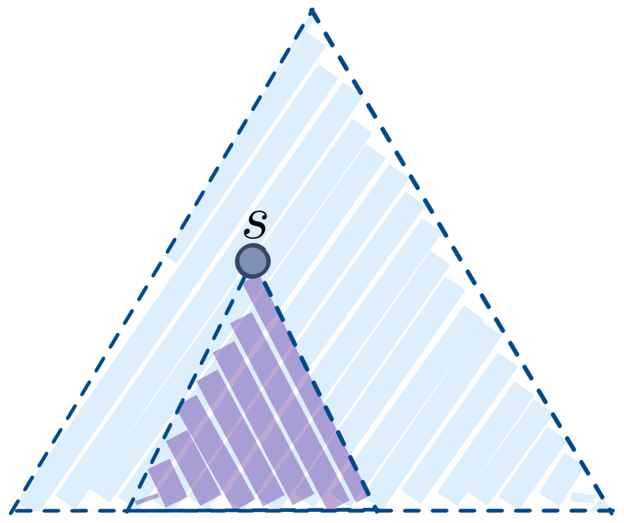
1-cut

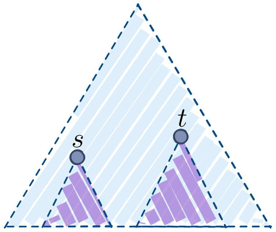
Incomparable 2-cut

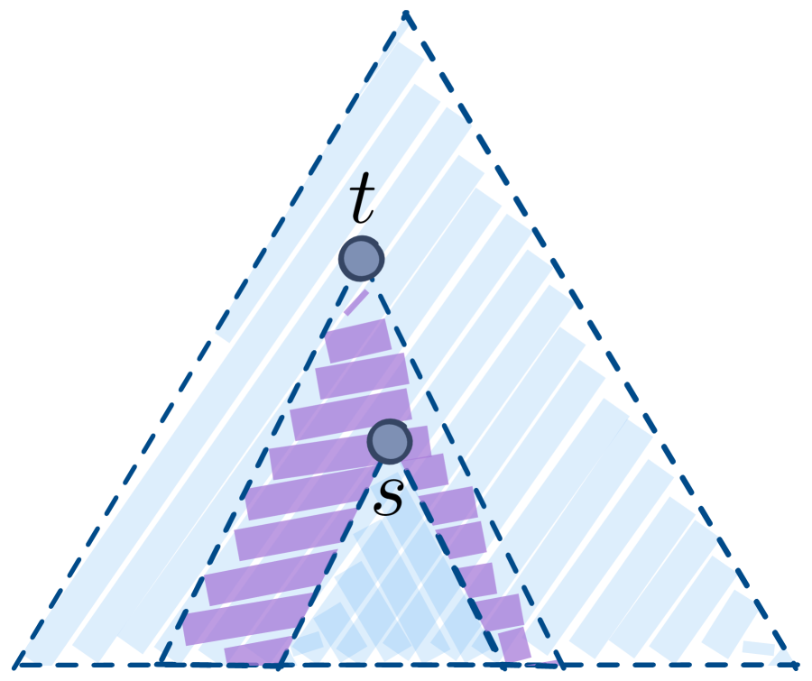
Nested 2-cut

Figure 6: 3 types of tree-cuts

Standard data structures.

Following Karger (2000), we rely on the dynamic tree data structure, link-cut trees, of Sleator and Tarjan (1983). Link-cut trees store real values at the nodes of a rooted tree $\displaystyle T$ and support aggregate operations along node-to-root paths in logarithmic time. We employ two operations in particular. First, given a node $\displaystyle v$ and a value $\displaystyle\alpha\in\mathbb{R}$, we can add $\displaystyle\alpha$ to the value of every node on the $\displaystyle v$-to-root path (i.e., every node $\displaystyle u$ such that $\displaystyle u\geq v$) in $\displaystyle O\left(\log n\right)$ amortized time. Second, given a node $\displaystyle v$, we can find the minimum value of any node on the $\displaystyle v$-to-root path in $\displaystyle O\left(\log n\right)$ amortized time.

We also need to compute least common ancestors ($\displaystyle\operatorname{{\texttt{lca}}}$) in $\displaystyle T$ for pairs of nodes. Harel and Tarjan (1984) showed how to preprocess $\displaystyle T$ in linear time and answer $\displaystyle\operatorname{{\texttt{lca}}}$ queries in constant time.

4.1 1-cuts

Let $\displaystyle e=(t,s)\in T$ be a tree edge with $\displaystyle t$ a parent of $\displaystyle s$. Then $\displaystyle T-e$ consists of two components: the subtree $\displaystyle T_{s}$ rooted at $\displaystyle s$, and the remaining tree $\displaystyle T\setminus T_{s}$. The cut $\displaystyle\mathscr{C}\left(D(s)\right)$ in the underlying graph $\displaystyle\mathcal{G}$ induced by the subtree $\displaystyle T_{s}$ is a ‘‘1-cut’’ of $\displaystyle T$. In this section, we want to output a sequence of 1-cuts $\displaystyle C\in\mathcal{C}_{T}$ in $\displaystyle T$ with $\displaystyle\overline{w}\left(C\right)\leq(1+O(\epsilon))\lambda$, repeating if necessary, while incrementing weights of each listed cut on the fly, until we’ve determined that there are no 1-cuts $\displaystyle C$ with weight $\displaystyle\overline{w}\left(C\right)\leq(1+\epsilon)\lambda$.

Computing and maintaining the 1-cut values.

To find the minimum 1-cut induced by a down set $\displaystyle D(v)$, Karger observes that the weight $\displaystyle\overline{\mathscr{C}}\left(D\left(v\right)\right)$ can be rewritten as

$$\displaystyle\overline{\mathscr{C}}\left(D\left(v\right)\right)=\sum_{x\in D(v)}\overline{\mathscr{C}}\left(x\right)-2\sum_{e\in\mathcal{E}[D(v)]}w_{e},$$

where $\displaystyle\overline{\mathscr{C}}\left(x\right)$ is the weighted degree of the vertex $\displaystyle x$, and $\displaystyle\mathcal{E}[D(v)]$ is the set of edges with both endpoints in $\displaystyle D(v)$.

The quantities $\sum_{x\in D(v)}\overline{\mathscr{C}}\left(x\right)$ over $\displaystyle v\in\mathcal{V}$ are just tree sums over the weighted degrees, and Karger (2000) computes them once for all $\displaystyle v$ in $\displaystyle O(m)$ total time by a depth-first traversal. In the dynamic setting, we can compute and maintain the tree sums in $\displaystyle O\left(\log n\right)$ time per edge update in a link-cut tree. Each time we increment the value of an edge $\displaystyle e=(u,v)\in\mathcal{E}$ by some $\displaystyle\delta>0$, we add $\displaystyle\delta$ to the value of every node on the paths to the root from $\displaystyle u$ and $\displaystyle v$.

The sum $\overline{w}\left(\mathcal{E}[D(v)]\right)\overset{\operatorname{def}}{=}\sum_{e\in\mathcal{E}[D(v)]}w_{e}$ over edges with both endpoints in $\displaystyle D(v)$ is just the sum of weights of all edges $\displaystyle e=(x,y)$ for which the least common ancestor $\displaystyle\operatorname{{\texttt{lca}}}\left(x,y\right)$ of $\displaystyle x$ and $\displaystyle y$ is in $\displaystyle D(v)$; i.e., $\overline{w}\left(\mathcal{E}[D(v)]\right)=\sum_{e:\operatorname{{\texttt{lca}}}\left(e\right)\in D(v)}w_{e}$ By Harel and Tarjan (1984), we can compute $\displaystyle\operatorname{{\texttt{lca}}}\left(e\right)$ for every edge $\displaystyle e\in\mathcal{E}$ in linear time. We then compute for each vertex $\displaystyle v$ the sum $\displaystyle\sum_{\operatorname{{\texttt{lca}}}\left(e\right)=v}w_{e}$ of all weights of edges whose least common ancestor is $\displaystyle v$. The quantities $\displaystyle\overline{w}\left(\mathcal{E}[(D(v))]\right)$ can then be computed as tree-sums by depth-first search, and updated dynamically with link-cut trees, similar to before.

The preceding discussion shows that the sums $\displaystyle\overline{\mathscr{C}}\left(D\left(v\right)\right)$ for each $\displaystyle v$ can be maintained dynamically in logarithmic time using link-cut trees. This is summarized in the lemma below.

Lemma 4.3.

Given edge-weighted graph $\displaystyle\mathcal{G}=\left(\mathcal{V},\mathcal{E}\right)$ and a rooted spanning tree $\displaystyle T$, there is a data structure to maintain $\displaystyle\overline{\mathscr{C}}\left(D(v)\right)$ for all $\displaystyle v\in\mathcal{V}$ as edge-weights are changed. The initialization cost is $\displaystyle O(m)$, updates and queries take $\displaystyle O\left(\log n\right)$ amortized time.

Processing all 1-cuts.

The weight of all 1-cuts can be computed in $\displaystyle O\left(m\right)$ time statically and $\displaystyle O\left(\log n\right)$-time per edge update. To process all 1-cuts of the tree, we consider all downsets $\displaystyle D(v)$ in any order. For each vertex $\displaystyle v$, we check if $\displaystyle\overline{\mathscr{C}}\left(D(v)\right)\leq(1+\epsilon)\lambda$ in $\displaystyle O\left(\log n\right)$ amortized time. If not, then we move on to the next vertex. Since the edge weights are monotonically increasing, $\displaystyle\overline{\mathscr{C}}\left(D(v)\right)$ will never be $\displaystyle\leq(1+\epsilon)\lambda$ again, so we do not revisit $\displaystyle v$. Otherwise, if $\displaystyle\mathscr{C}\left(D(v)\right)$ is good, we take the cut in our solution and pass $\displaystyle v$ to inc-cut to signal a weight increment along $\displaystyle\mathscr{C}\left(D(v)\right)$. In turn, inc-cut returns a list of ‘‘official’’ edge increments $\displaystyle\left\{(e_{i},\delta_{i})\right\}$. Each update can be incorporated into the link-cut tree in logarithmic time by Lemma 4.3. After processing the edge increments returned by inc-cut, we continue to process $\displaystyle D(v)$ until $\displaystyle\mathscr{C}\left(D(v)\right)$ is no longer a good cut. The total running time to process all 1-cuts is $\displaystyle O\left(m\right)$ plus $\displaystyle O\left(\log^{2}n\right)$ per cut output and $\displaystyle O\left(\log n\right)$ per edge weight increment returned by inc-cut.

Lemma 4.4.

Let $\displaystyle T$ be a fixed and rooted spanning tree and $\displaystyle\lambda>0$ a fixed target cut value. Employing the inc-cut routine of the lazy-inc-cuts data structure to approximately increment edge weights, one can repeatedly find 1-cuts $\displaystyle C$ induced by $\displaystyle T$ of value $\displaystyle\overline{\mathscr{C}}\left(C\right)\leq(1+O(\epsilon))\lambda$ and increment the corresponding edge weights (per the MWU framework) until certifying that there are no 1-cuts $\displaystyle C$ of value $\displaystyle\overline{\mathscr{C}}\left(C\right)\leq(1+\epsilon)\lambda$ in $\displaystyle O\left(m+K\log^{2}n+I\log n\right)$ total running time, where $\displaystyle K$ is the number of 1-cuts of value $\displaystyle\leq(1+O(\epsilon))$ output and $\displaystyle I$ is the total number of weight increments returned by inc-cut.

4.2 2-cuts on incomparable vertices

In this section, we consider incomparable 2-cuts of the form $\displaystyle\mathscr{C}\left(D(s)\cup D(t)\right)$, where $\displaystyle s\parallel t$. We first consider the case where $\displaystyle s$ is a fixed leaf, and $\displaystyle t$ ranges over all vertices incomparable to $\displaystyle s$. We then extend the leaf case to consider the case where $\displaystyle s$ ranges over a path in the tree down to a leaf, and $\displaystyle t$ ranges over all incomparable vertices to the path. We then apply an induction step that reduces processing the whole tree to a logarithmic number of rounds where in each round we process all the paths to leaves. See Figure 7.

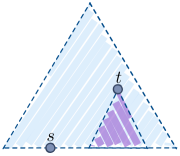
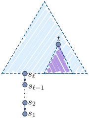
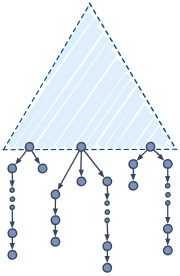
Fixed leaf

Fixed path to a leaf

Induction step

Figure 7: 3 cases for incomparable 2-cuts

Incomparable 2-cuts with a leaf.

We first fix $\displaystyle s$ to be a leaf in $\displaystyle T$, and consider all incomparable 2-cuts with one side fixed to be $\displaystyle\left\{s\right\}$. Karger observes that the weight of the cut induced by $\displaystyle D(t)+s$, for $\displaystyle t\parallel s$, can be written as

$$\displaystyle\overline{\mathscr{C}}\left(D(t)+s\right)=\overline{\mathscr{C}}\left(s\right)+\overline{\mathscr{C}}\left(D(t)\right)-2\overline{\mathscr{C}}\left(D(t),s\right)$$

where $\displaystyle\overline{\mathscr{C}}(D(t),s)$ is the weight of edges with one endpoint $\displaystyle s$ and the other in $\displaystyle D(t)$. We only need to consider down sets $\displaystyle D(t)$ for which $\displaystyle s$ and $\displaystyle D(t)$ are connected by some edge, since otherwise either $\displaystyle\left\{s\right\}$ or $\displaystyle D(t)$ induce a smaller cut, and after processing all 1-cuts, neither $\displaystyle\left\{s\right\}$ or $\displaystyle D(t)$ induce small enough cuts.

For fixed $\displaystyle s$ and ranging $\displaystyle t$ over all $\displaystyle t\parallel s$, Karger finds the weight of the best incomparable $\displaystyle D(t)+s$ cut statically as follows. As $\displaystyle\overline{\mathscr{C}}\left(s\right)$ is fixed, the $\displaystyle t$’s are differentiated only by the values $\overline{\mathscr{C}}\left(D(t)\right)-2\overline{\mathscr{C}}\left(D(t),s\right).$ Karger’s algorithm creates a dynamic tree over $\displaystyle T$ with each vertex $\displaystyle t$ initialized with the value $\displaystyle\overline{\mathscr{C}}\left(D(t)\right)$. (This initial tree only needs to be constructed once, and immutably reused for other $\displaystyle s$’s). Karger’s algorithm immediately adds $\displaystyle+\infty$ to the value of every vertex on the $\displaystyle s$-to-root path to eliminate all comparable vertices from consideration. For each edge $\displaystyle e=(s,v)$ with endpoint $\displaystyle s$, Karger’s algorithm subtracts $\displaystyle 2w_{e}$ from every vertex on the $\displaystyle v$-to-root path, to incorporate the second term $\displaystyle-2\overline{\mathscr{C}}\left(D(t),s\right)$. Then, for each edge $\displaystyle e=(s,v)$ adjacent to $\displaystyle s$, Karger’s algorithm finds the minimum value vertex on the $\displaystyle v$ to root path. The minimum value vertex $\displaystyle z$ over all such queries gives the best $\displaystyle s+D(z)$ cut subject to $\displaystyle s\parallel z$, as desired. The running time to process the leaf $\displaystyle s$, excluding the construction of the initial tree, is bounded by the time spent subtracting edge weights and taking minimums over the $\displaystyle v$-to-root path for each edge $\displaystyle(s,v)$ incident to $\displaystyle s$. With dynamic trees, subtracting and finding the minimum along a vertex-to-root path each take $\displaystyle O\left(\log n\right)$ amortized time. Thus, up to a logarithmic factor, the time spent processing all incomparable 2-cuts with one side a fixed leaf $\displaystyle s$ is proportional to the number of edges incident to $\displaystyle s$.

In the dynamic setting, we do the following. We first compute the sum $\displaystyle\overline{\mathscr{C}}\left(D(t)\right)-2\overline{\mathscr{C}}\left(D(t),s\right)$ for all incomparable $\displaystyle t:t\parallel s$, as above. We then run through the edges $\displaystyle(s,v)$ incident to $\displaystyle s$ in any fixed order, checking for $\displaystyle s+D(t)$ cuts with $\displaystyle t\geq v$ that have value $\displaystyle\leq(1+\epsilon)\lambda$ and updating edge weights along good cuts on the fly, as follows.

Fix an edge $\displaystyle e=(s,v)$ incident to $\displaystyle s$. We process $\displaystyle e$ until we know that there is no good $\displaystyle(D(t)+s)$-cut for any ancestor $\displaystyle t$ of $\displaystyle v$. We first find the minimum value vertex on the $\displaystyle v$-to-root path in $\displaystyle O\left(\log n\right)$ amortized time. If the minimum value is $\displaystyle>(1+\epsilon)\lambda-\overline{\mathscr{C}}\left(D(s)\right)$, then we move onto the next edge incident to $\displaystyle s$. Otherwise, let $\displaystyle t$ be an ancestor of $\displaystyle v$ such that $\displaystyle s+D(t)$ induces a good cut. We pass the cut $\displaystyle\mathscr{C}\left(s+D(t)\right)$ (in terms of the roots of $\displaystyle s$ and $\displaystyle t$) to inc-cut, which simulates a weight update along $\displaystyle\mathscr{C}\left(s+D(t)\right)$ and returns a list of weight increments $\displaystyle\left\{(e_{i},\delta_{i})\right\}$. For each such edge $\displaystyle e=(x,y)$ whose weight is increased by some $\displaystyle\delta>0$, we add $\displaystyle\delta$ to every vertex on the $\displaystyle x$-to-root and $\displaystyle y$-to-root paths. We then subtract $\displaystyle 2\delta$ from the $\displaystyle\operatorname{{\texttt{lca}}}\left(x,y\right)$-to-root path. These additions and subtraction account for the first term, $\displaystyle\overline{\mathscr{C}}\left(D(t)\right)$. If $\displaystyle x=s$, then we also subtract $\displaystyle 2\delta$ from the $\displaystyle y$-to-root path for the sake of the second term, $\displaystyle-2\overline{\mathscr{C}}\left(D(t),s\right)$. After all official weight increments returned by inc-cut have been incoporated into the dynamic tree, we continue to process the same edge $\displaystyle e=(s,v)$. Once all edges $\displaystyle e=(s,v)$ incident to $\displaystyle s$ have been processed, we have certified that all 2-cuts with one side fixed to the leaf $\displaystyle s$ have weight $\displaystyle\geq(1+\epsilon)\lambda$. The total time is $\displaystyle O\left(\log n\right)$ times the number of edges incident to $\displaystyle s$, plus $\displaystyle O\left(\log^{2}n\right)$ time for every cut output and $\displaystyle O\left(\log n\right)$ for every increment returned by inc-cut.

Leaf-paths.

The approach outlined above for processing leaves extends to processing paths. Let a leaf-path be a maximal subtree that is a path. Let $\displaystyle p=s_{1},s_{2},\dots,s_{\ell}$ be a leaf path, where $\displaystyle s_{1}$ is a leaf, $\displaystyle s_{2}$ is its parent, and so forth. We want to process all 1-cuts of the form $\displaystyle D(s_{i})\cup D(t)$, where $\displaystyle t$ is incomparable to any and all of the $\displaystyle s_{i}$’s on the path.

For each $\displaystyle i$, we have

$$\displaystyle\overline{\mathscr{C}}\left(D(s_{i})\cup D(t)\right)=\overline{\mathscr{C}}\left(D(s_{i})\right)+\overline{\mathscr{C}}\left(D(t)\right)-2\overline{\mathscr{C}}\left(D(s_{i}),D(t)\right),$$

where $\displaystyle\overline{\mathscr{C}}\left(D(s_{i}),D(t)\right)$ is the weight of all edges between $\displaystyle D(s_{i})$ and $\displaystyle D(t)$. The values $\displaystyle\overline{\mathscr{C}}\left(D(t)\right)$ for $\displaystyle t\parallel s_{1},\dots,s_{\ell}$ and $\displaystyle\overline{\mathscr{C}}\left(D(s_{i})\right)$ for each $\displaystyle i$ are easy to compute initially and maintain dynamically, per the earlier discussion about 1-cuts in Section 4.1. For fixed $\displaystyle i$, the incomparable $\displaystyle t$ are differentiated by the value $\displaystyle\overline{\mathscr{C}}\left(D(t)\right)-2\overline{\mathscr{C}}\left(D(s_{i}),D(t)\right)$. The basic idea here is that $\displaystyle\overline{\mathscr{C}}\left(D(s_{i+1}),D(t)\right)$ can be written in terms of the preceding cut in the form $\overline{\mathscr{C}}\left(D(s_{i+1}),D(t)\right)=\overline{\mathscr{C}}\left(D(s_{i}),D(t)\right)+\overline{\mathscr{C}}\left(s_{i+1},D(t)\right).$ That is, after computing $\displaystyle\overline{\mathscr{C}}\left(D(s_{i}),D(t)\right)$ for all incomparable $\displaystyle t$, we can keep these values and just incorporate the weights of edges incident to $\displaystyle s_{i+1}$ to get the values $\displaystyle\overline{\mathscr{C}}\left(D(s_{i}),D(t)\right)$ for all incomparable $\displaystyle t$.

We first review the static case, where we want to find the minimum such cut. Karger’s algorithm first processes the leaf $\displaystyle s_{1}$ as a leaf, as outlined above, and takes note of the minimum $\displaystyle s_{1}+D(t)$ cut. It then processes $\displaystyle s_{2}$ in the same fashion, except it continues the aggregate data built when processing $\displaystyle s_{1}$ rather than starting fresh. By subtracting the weights of all edges incident $\displaystyle s_{2}$ from the values of the various incomparable downsets, and having already subtracted the weights of edges incident to $\displaystyle s_{1}$, we will have subtracted the weight of all edges incident to $\displaystyle D(s_{2})=\left\{s_{1},s_{2}\right\}$, and so we have computed $\displaystyle\overline{\mathscr{C}}\left(D(t)\right)-2\overline{\mathscr{C}}\left(D(s_{2}),D(t)\right)$ for all $\displaystyle t\parallel s_{2}$. In this fashion, Karger’s algorithm marches up the path doing essentially the same work for each vertex as for a fixed leaf, except continuing the same link-cut tree from one $\displaystyle s_{i}$ to the next. The total work processing the entire leaf-path is, up to a logarithmic factor, proportional to the total number of edges incident to any node $\displaystyle s_{i}$ on the path.

The analogous adjustments are made in the dynamic setting. That is, we process $\displaystyle s_{1}$ as a leaf, passing good cuts to inc-cut and incorporating the returned edge increments on the fly. After processing $\displaystyle s_{1}$, we keep the accumulated aggregate values, and start processing $\displaystyle s_{2}$ likewise. Marching up the leaf-path one vertex at a time. In this manner, we are able to process 2-cuts of the form $\displaystyle D(s_{i})+D(t)$ over each $\displaystyle s_{i}$ along the leaf-path $\displaystyle s_{1},\dots,s_{\ell}$ (subject to $\displaystyle t\parallel s_{1},\dots,s_{\ell}$) and at the end certify there are no such cuts of weight $\displaystyle<(1+\epsilon)\lambda$. The total work in processing the leaf path is $\displaystyle O\left(\log n\right)$ for each edge incident to $\displaystyle s_{1},\dots,s_{\ell}$, $\displaystyle O\left(\log^{2}n\right)$ for each good cut output, and $\displaystyle O\left(\log n\right)$ for each weight increment returned from the subroutine inc-cut.

All incomparable 2-cuts.

Karger (2000) showed that an efficient subroutine for processing all incomparable 2-cuts on a single leaf-path leads to an efficient algorithm for processing all incomparable 2-cuts in the entire tree as follows. The overall algorithm processes the 2-cuts of a tree in phases. Each phase processes all the leaf-paths of the current tree, and then contracts the leaf-paths into their parents and recurses on the new tree in a new phase. Each leaf in the contracted graph had at least two children in the previous phase, so the number of nodes has halved. After at most $\displaystyle O(\log n)$ phases, we have processed all the incomparable 2-cuts in the tree. Excluding the work for selecting a cut and incrementing edge weights returned by the lazy-inc-cuts data structure, processing a leaf-path takes time proportional to the number of edges incident to the leaf-path. Each edge is incident to at most 2 leaf-paths. Thus, a single phase takes $\displaystyle O\left(m\log n\right)$ time, in addition to $\displaystyle O\left(\log^{2}n\right)$ time for every cut output and $\displaystyle O\left(\log n\right)$ amortized time for every edge weight increment returned by the lazy-inc-cuts data structure. In conclusion, we have shown the following.

Lemma 4.5.

Let $\displaystyle T$ be a fixed and rooted spanning tree and $\displaystyle\lambda>0$ a fixed target cut value. Employing the inc-cut routine of the lazy-inc-cuts data structure to approximately increment edge weights, one can repeatedly find incomparable 2-cuts $\displaystyle C$ induced by $\displaystyle T$ of value $\displaystyle\overline{\mathscr{C}}\left(C\right)\leq(1+O(\epsilon))\lambda$ and increment the corresponding edge weights (per the MWU framework) until certifying that there are no incomparable 2-cuts $\displaystyle C$ of value $\displaystyle\overline{\mathscr{C}}\left(C\right)\leq(1+\epsilon)\lambda$ in $\displaystyle O\left(m\log^{2}n+K\log^{2}n+I\log n\right)$ total amortized time, where $\displaystyle K$ is the number of incomparable 2-cuts of value $\displaystyle\leq(1+O(\epsilon))\lambda$ output and $\displaystyle I$ is the total number of weight increments returned by inc-cut.

4.3 Nested 2-cuts

The other type of 2-cuts is of the form $\displaystyle D(t)\setminus D(s)$, where $\displaystyle t$ is an ancestor of $\displaystyle s$. We call these cuts nested 2-cuts. As in the case of incomparable 2-cuts, we first consider the case where $\displaystyle s$ is fixed to be a leaf, then the case where $\displaystyle s$ is on a leaf-path, and then finally an induction step that processes all leaf-paths in each pass.

Nested 2-cuts with a leaf.

We take the same approach as with incomparable 2-cuts, and start with the case where $\displaystyle s$ is a fixed leaf. Karger observed that the weight of the cut induced by $\displaystyle D(t)-s$ can be written as

(1) $$\displaystyle\overline{\mathscr{C}}\left(D(t)-s\right)=\overline{\mathscr{C}}\left(D(t)\right)+2\overline{\mathscr{C}}\left(s,D(t)\right)-\overline{\mathscr{C}}\left(s\right),$$

where $\displaystyle\overline{\mathscr{C}}\left(s,D(t)\right)$ is the sum weight of the edges between $\displaystyle s$ and $\displaystyle D(t)$. We start with a link-cut tree over $\displaystyle T$ where each node $\displaystyle v$ is initialized with $\displaystyle\overline{\mathscr{C}}\left(D(v)\right)$. For each edge $\displaystyle e=(s,u)$ incident to $\displaystyle s$, we find the least common ancestor $\displaystyle t=\operatorname{{\texttt{lca}}}\left(s,u\right)$, and add $\displaystyle 2w_{e}$ to every node on the $\displaystyle u$-to-root path in $\displaystyle O\left(\log n\right)$ time. We also subtract $\displaystyle w_{e}$ from the value of every node on the $\displaystyle s$-to-root path. The first set of updates along the $\displaystyle t$-to-root path is for the second term of (1), and the second set along the $\displaystyle s$-to-root path is for the third term.

Karger’s algorithm finds the minimum value on the $\displaystyle s$-to-root path to get the value of the minimum $\displaystyle(D(t)-s)$-cut over all $\displaystyle t>s$. In the dynamic setting, we repeatedly find the minimum value on the $\displaystyle s$-to-root path as long as this value is below the threshold $\displaystyle(1+\epsilon)\lambda$. Each time we find a good cut $\displaystyle\mathscr{C}\left(D(t)-s\right)$, we send the cut to the routine inc-cut (compactly represented by $\displaystyle s$ and $\displaystyle t$). For each edge weight increment $\displaystyle(e=(x,y),\delta)$ returned by inc-cut we do the following. Let $\displaystyle t=\operatorname{{\texttt{lca}}}\left(x\right){y}$ be the least common ancestor. First, we add $\displaystyle\delta$ to every the value of every vertex on the $\displaystyle x$-to-root and $\displaystyle y$-to-root paths and subtract $\displaystyle 2\delta$ from every value of every vertex on the $\displaystyle t$-to-root-path in $\displaystyle O(\log n)$ time, to account for the first term $\displaystyle\overline{\mathscr{C}}\left(D(t)\right)$ (see Section 4.1). If $\displaystyle e$ is also incident to $\displaystyle s$, then we add $\displaystyle 2\delta$ to the value of every vertex on the $\displaystyle t$-to-root path (for the second term of (1)), and subtract $\displaystyle\delta$ from the value of every vertex on the $\displaystyle s$-to-root path (for the third term). Thus, incorporating an edge increment $\displaystyle(e,\delta)$ consists of a constant number of updates along node-to-root paths and takes $\displaystyle O\left(\log n\right)$ amortized time.

The total amortized running time for processing all nested 2-cuts of the form $\displaystyle D(t)-s$ with a fixed leaf $\displaystyle s$ is $\displaystyle O\left(\log n\right)$ times the number of edges incident to $\displaystyle s$, plus $\displaystyle O\left(\log^{2}n\right)$ for every cut output and $\displaystyle O\left(\log n\right)$ for every edge weight increment returned by the inc-cut subroutine.

Nested 2-cuts along a leaf-path.

We extend the leaf case to a leaf path $\displaystyle s_{1},\dots,s_{\ell}$, where $\displaystyle s_{1}$ is a leaf and each $\displaystyle s_{i}$ with $\displaystyle i>1$ has exactly one child, and consider all cuts of the form $\displaystyle D(t)\setminus D(s_{i})$ over all $\displaystyle s_{i}$ in the leaf path and all ancestors $\displaystyle t$ of $\displaystyle s_{i}$. For each $\displaystyle i$, we have

(2) $$\displaystyle\overline{\mathscr{C}}\left(D(t)\setminus D(s_{i})\right) \displaystyle=\overline{\mathscr{C}}\left(D(t)\right)+2\overline{\mathscr{C}}\left(D(s_{i}),D(t)\right)-\overline{\mathscr{C}}\left(D(s_{i})\right).$$

When $\displaystyle i=1$, this is the same as equation (1) obtained for the leaf case. For $\displaystyle i=1,\dots,\ell-1$, the difference in (2) between consecutive vertices $\displaystyle s_{i}$ and $\displaystyle s_{i+1}$ is

$$\displaystyle\overline{\mathscr{C}}\left(D(t)\setminus D(s_{i+1})\right)-\overline{\mathscr{C}}\left(D(t)\setminus D(s_{i})\right)$$

$$\displaystyle=2\left[\overline{\mathscr{C}}\left(D(s_{i+1}),D(t)\right)-\overline{\mathscr{C}}\left(D(s_{i}),D(t)\right)\right]-\left[\overline{\mathscr{C}}\left(D(s_{i+1})-\overline{\mathscr{C}}\left(D(s_{i})\right)\right)\right]$$

(3) $$\displaystyle=2\overline{\mathscr{C}}\left(s_{i+1},D(t)\right)+\overline{\mathscr{C}}\left(s_{i+1}\right)-2\overline{\mathscr{C}}\left(s_{i+1},D(s_{i})\right).$$

These observations lead to the following bottom-up approach. We first process $\displaystyle s_{1}$ as though it were a leaf, as described above. For $\displaystyle i=1,\dots,\ell-1$, once we have certified that are no nested $\displaystyle D(t)-s_{i}$ cuts of value $\displaystyle<(1+\epsilon)\lambda$, we begin to process $\displaystyle s_{i+1}$, continuing the aggregate values computed when processing $\displaystyle s_{i}$ instead of starting over. For each edge $\displaystyle e=(s_{i+1},x)$ incident to $\displaystyle s_{i+1}$, we update the values along paths up the tree per (3) as follows. For the first term, $\displaystyle 2\overline{\mathscr{C}}\left(s_{i+1},D(t)\right)$, we find the least common ancestor $\displaystyle t=\operatorname{{\texttt{lca}}}\left(s_{i+1},x\right)$, and add $\displaystyle 2w_{e}$ to every vertex on the $\displaystyle t$-to-root path. For the second term, $\displaystyle\overline{\mathscr{C}}\left(s_{i+1}\right)$, we add $\displaystyle w_{e}$ to every vertex on the $\displaystyle s_{i+1}$-to-root path. For the third term, $\displaystyle 2\overline{\mathscr{C}}\left(s_{i+1},D(S_{i})\right)$, if $\displaystyle x=s_{j}$ for some $\displaystyle j<i$, then we subtract $\displaystyle 2w_{e}$ from every vertex on the $\displaystyle s_{i+1}$-to-root path. After processing the edges incident to $\displaystyle s_{i+1}$, we repeatedly find the minimum value in the $\displaystyle s_{i+1}$-to-root path so long as the minimum value is less than the threshold $\displaystyle\left(1+\epsilon\right)\lambda$. Each time the minimum value is below the threshold, we update weights along the edges of the corresponding cut via inc-cut, and propagate any increments returned by inc-cut (as before) to restore (2) before querying for the next minimum value.

To process all the nested 2-cuts along the leaf-path, as with incomparable 2-cuts along leaf-paths, the total amortized running time is $\displaystyle O(\log n)$ times the number of edges incident to $\displaystyle s_{1},\dots,s_{\ell}$, plus $\displaystyle O\left(\log^{2}n\right)$ work for each cut output and $\displaystyle O\left(\log n\right)$ work for each edge increment returned by inc-cut.

All nested 2-cuts.

By the same induction step as for incomparable 2-cuts, efficiently processing leaf-paths leads to a procedure for efficiently processing the whole tree. The processing is broken into phases. Each phase processes all the leaf-paths of the current tree, and then contracts the leaf-paths into their parents. Each leaf in the contracted tree had at least two children previously, so the number of nodes has at least halved. After $\displaystyle O(\log n)$ phases, we have processed the entire tree. Modulo $\displaystyle O\left(\log^{2}n\right)$ work for each cut output and $\displaystyle O\left(\log n\right)$ work for each edge increment returned by inc-cut, processing a leaf path takes $\displaystyle O\left(\log n\right)$ time for each edge incident to any node on the path, and conversely each edge is incident to at most 2 leaf paths. Thus, excluding the time spent outputting cuts and incrementing edge weights along the cuts, each phase takes $\displaystyle O\left(m\log n\right)$ to complete.

Lemma 4.6.

Let $\displaystyle T$ be a fixed and rooted spanning tree and $\displaystyle\lambda>0$ a fixed target cut value. Employing the inc-cut routing of the lazy-inc-cuts data structure to manage edge weight increments, one can repeatedly find nested 2-cuts $\displaystyle C$ induced by $\displaystyle T$ of value $\displaystyle\overline{\mathscr{C}}\left(C\right)\leq(1+O(\epsilon))\lambda$ and increment the corresponding edge weights (per the MWU framework) until certifying that there are no incomparable 2-cuts $\displaystyle C$ of value $\displaystyle\overline{\mathscr{C}}\left(C\right)\leq(1+\epsilon)\lambda$, in $\displaystyle O\left(m\log^{2}n+K\log^{2}n+I\log n\right)$ total running time, where $\displaystyle K$ is the number of nested 2-cuts of value $\displaystyle\leq(1+O(\epsilon))\lambda$ output and $\displaystyle I$ is the total number of weight increments returned by inc-cut.

5 Applying multiplicative weight updates along cuts

We address the remaining issue of implementing the lazy-inc-cuts data structure for a fixed and rooted spanning tree $\displaystyle T$. An interface for lazy-inc-cuts was given previously in Figure 4 and we target the bounds claimed by Lemma 4.1. Recall that the MWU framework takes a cut $\displaystyle C\in\mathcal{C}$, computes the smallest capacity $\displaystyle\gamma=\operatorname*{arg\,min}_{e\in C}c_{e}$ in the cut, and increases the weight of each cut-edge $\displaystyle e\in C$ by a multiplicative factor of $\displaystyle\exp\left(\epsilon\gamma/c_{e}\right)$ (see Figure 1). A subtle point is that the techniques of Section 4 identify approximate min-cuts without explicitly listing the edges in the cut. A 1-cut $\displaystyle\mathscr{C}\left(D(s)\right)$ is simply identified by the root $\displaystyle s$ of the down-set $\displaystyle D(s)$, and likewise 2-cuts of the form $\displaystyle\mathscr{C}\left(D(s)\cup D(t)\right)$ (when $\displaystyle s\parallel t$) and $\displaystyle\mathscr{C}\left(D(t)\setminus D(s)\right)$ (when $\displaystyle s<t$) can be described by the two nodes $\displaystyle s$ and $\displaystyle t$. In particular, an approximately minimum cut $\displaystyle C$ is identified without paying for the number of edges $\displaystyle O\left(\left|C\right|\right)$ in $\displaystyle C$ in the running time. When it comes to updating the edge weights, the natural approach of visiting each edge $\displaystyle e\in C$ would be too slow, to say nothing of even identifying all the edges in $\displaystyle C$ in time proportional to $\displaystyle\left|C\right|$.

While the general task of incrementing weights along a cut appears difficult to execute both quickly and exactly, we have already massaged the setting to be substantially easier. First, we can afford to approximate the edge weights $\displaystyle w_{e}$ by a small multiplicative error. This means, for example, that a cut edge $\displaystyle e\in C$ with very large capacity $\displaystyle c_{e}\gg\gamma$ can to some extent be ignored. Second, we are not incrementing weights along any cut, but just the 1-cuts and 2-cuts of a fixed rooted spanning tree $\displaystyle T$. We have already seen in Section 4 that restricting ourselves to 1-cuts and 2-cuts allows us to (basically) apply dynamic programming to find small cuts, and also allows us to use dynamic trees to efficiently update and scan various values in the aggregate. Here too we will see that 1-cuts and 2-cuts are simple enough to be represented efficiently in standard data structures. In the following, we use the term ‘‘cuts’’ liberally as the set of edges with endpoints in each of two sets of vertices; in particular, the two sets of vertices may not be disjoint.

Lemma 5.1.

Let $\displaystyle T$ be a fixed rooted spanning tree of an undirected graph $\displaystyle\mathcal{G}=\left(\mathcal{V},\mathcal{E}\right)$ with $\displaystyle\left|\mathcal{E}\right|=m$ edges and $\displaystyle\left|\mathcal{V}\right|=n$ vertices. In $\displaystyle O\left(m\log^{2}n\right)$ time, one can construct a collection of nonempty cuts $\displaystyle\mathcal{D}_{T}\subseteq 2^{\mathcal{E}}$ such that

1. every edge $\displaystyle e\in\mathcal{E}$ appears in at most $\displaystyle O(\log^{2}n)$ cuts $\displaystyle D\in\mathcal{D}_{T}$, and

2. every 1-cut or 2-cut $\displaystyle C\in\mathcal{C}_{T}$ (described succinctly by at most 2 roots of subtrees) can be decomposed into the disjoint union $C=D_{1}\sqcup\cdots\sqcup D_{\ell}$ of $\displaystyle\ell=O(\log^{2}n)$ cuts $\displaystyle D_{1},\dots,D_{\ell}\in\mathcal{D}_{T}$ in $\displaystyle O(\log^{2}n)$ time.

By building the collection $\displaystyle D\in\mathcal{D}_{T}$ once for a tree $\displaystyle T$, Lemma 5.1 reduces the problem of incrementing along any 1-cut or 2-cut $\displaystyle C\in\mathcal{C}_{T}$ to incrementing along a ‘‘canonical’’ cut $\displaystyle D\in\mathcal{D}_{T}$ known a priori. This is important because multiplicative weight updates can be applied to a static set relatively efficiently by known techniques (Young, 2014; Chekuri and Quanrud, 2017b). It is also important that cuts in $\displaystyle\mathcal{D}_{T}$ are sparse, in the sense that $\displaystyle\sum_{D\in\mathcal{D}_{T}}\left|D\right|=O\left(m\log^{2}n\right)$, as this sum factors directly into the running time guarantees. We first prove Lemma 5.1 in Section 5.1, and then in Section 5.2 we show how to combine amortized data structures for each $\displaystyle D\in\mathcal{D}_{T}$ to increment along any 1-cut or 2-cut $\displaystyle C\in\mathcal{C}_{T}$.

5.1 Canonical cuts

An Euler tour inducing the ordering $r^{-}<a^{-}<a^{+}<b^{-}<c^{-}<c^{+}<d^{-}<d^{+}<b^{+}<r^{+}.$

Euler tours and orderings. Let $\displaystyle T$ be a fixed and rooted tree on $\displaystyle n$ vertices $\displaystyle\mathcal{V}$, and fix an Euler tour on a bidirected copy of $\displaystyle T$ that replaces each edge of $\displaystyle T$ with arcs in both directions, starting from the root. For each vertex $\displaystyle v$, we create two symbols: $\displaystyle v^{-}$ means we enter the subtree $\displaystyle T_{v}$ rooted at $\displaystyle v$, and $\displaystyle v^{+}$ means we leave the subtree $\displaystyle v$. Let $\mathcal{V}^{\pm}=\left\{v^{-},v^{+}:v\in\mathcal{V}\left(T\right)\right\}$ denote the whole collection of these $\displaystyle 2n$ symbols. The Euler tour enters and leaves each subtree exactly once in a fixed order. Tracing the Euler tree induces a unique total ordering on $\displaystyle\mathcal{V}^{\pm}$ (see the picture on the right).

This ordering has a couple of interesting properties. For every vertex $\displaystyle v\in\mathcal{V}(T)$, we have $\displaystyle v^{-}<v^{+}$. Letting $\displaystyle r$ denote the root of $\displaystyle T$, $\displaystyle r^{-}$ is the first element in the ordering and $\displaystyle r^{+}$ is the last element in the ordering. More generally, for a vertex $\displaystyle v$ and a vertex $\displaystyle w\in D(v)$ in the subtree rooted at $\displaystyle v$, we have $\displaystyle v^{-}\leq w^{-}<w^{+}\leq v^{+}$, with all inequalities strict if $\displaystyle v\neq w$. That is, the ranges $\displaystyle\left\{[v^{-},v^{+}]:v\in\mathcal{V}(T)\right\}$ between entering and leaving a subtree form a laminar set.

The Euler order on the vertices endows a sort of geometry to the edges. Each edge $\displaystyle e=(u,v)$ (with $\displaystyle u^{-}<v^{-}$) can be thought of as an interval $\displaystyle[u^{-},v^{-}]$. A downset $\displaystyle D(s)$ cuts $\displaystyle e$ iff $u^{-}\leq s^{-}\leq v^{-}\leq s^{+}$ or $s^{-}\leq u^{-}\leq s^{+}\leq v^{-}$ (see Figure 8); that is, iff $\left|\left\{u^{-},v^{-}\right\}\cap[s^{-},s^{+}]\right|=1.$ Alternatively, $\displaystyle D(s)$ cuts $\displaystyle e$ iff $\left|[u^{-},v^{-}]\cap\left\{s^{-},s^{+}\right\}\right|=1.$ These observations suggest that this is not a problem about graphs, but about intervals, and perhaps a problem suited for range trees.

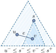
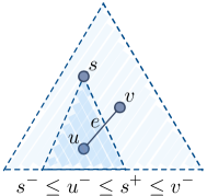
Figure 8: An edge cut $\displaystyle e$ by a subtree $\displaystyle T_{s}$, and two possible inequalities in the Euler order.

Range trees on the Euler order.

Let $\displaystyle R$ be a balanced range tree with $\displaystyle\mathcal{V}^{\pm}$ at its leaves. As a balanced tree with $\displaystyle 2n$ leaves, $\displaystyle R$ has $\displaystyle O\left(n\right)$ nodes and height $\displaystyle O(\log n)$. Each range-node $\displaystyle a\in\mathcal{V}\left(R\right)$ induces an interval $\displaystyle I_{a}$ on $\displaystyle\mathcal{V}^{\pm}$, consisting of all the elements of $\displaystyle\mathcal{V}^{\pm}$ at the leaves of the subtree $\displaystyle R_{a}$ rooted at $\displaystyle a$. We call $\displaystyle I_{a}$ a canonical interval of $\displaystyle\mathcal{V}^{\pm}$ (induced by $\displaystyle a$), and let $\displaystyle\mathcal{I}=\left\{I_{a}:a\in\mathcal{V}(R)\right\}$ denote the collection of all $\displaystyle O(n)$ canonical intervals.

Each element in $\displaystyle\mathcal{V}^{\pm}$ appears in $\displaystyle O(\log n)$ canonical intervals because the height of $\displaystyle R$ is $\displaystyle O(\log n)$. Moreover, every interval $\displaystyle J$ on $\displaystyle\mathcal{V}^{\pm}$ decomposes into the disjoint union of $\displaystyle O(\log n)$ canonical intervals. The decomposition can be obtained in $\displaystyle O(\log n)$ time by tracing the two paths from the root of $\displaystyle R$ to the endpoints of $\displaystyle J$ and taking the canonical intervals corresponding to the $\displaystyle O(\log n)$ maximal subtrees between the paths (see the picture on the right). Similarly, the union of a constant number of intervals or the complement of the union of a constant number of intervals decomposes to $\displaystyle O(\log n)$ canonical intervals in $\displaystyle O(\log n)$ time.

The canonical intervals $\displaystyle\mathcal{I}$ relate to the 1-cuts and 2-cuts $\displaystyle\mathcal{C}_{T}$ induced by $\displaystyle T$ as follows. For any pair of disjoint canonical intervals $\displaystyle I_{1},I_{2}\in\mathcal{I}$, let $\mathscr{C}\left(I_{1},I_{2}\right)=\left\{(u,v)\in\mathcal{E}:u\in I_{1},v\in I_{2}\right\}$ be the set of edges with one endpoint in $\displaystyle I_{1}$ and the other in $\displaystyle I_{2}$. We call $\displaystyle\mathscr{C}\left(I_{1},I_{2}\right)$ a canonical cut induced by $\displaystyle I_{1}$ and $\displaystyle I_{2}$. We claim that any 1-cut or 2-cut $\displaystyle C\in\mathcal{C}_{T}$ decomposes into the disjoint union of $\displaystyle O(\log^{2}n)$ canonical cuts.

For starters, let $\displaystyle C=\mathscr{C}\left(D(s)\right)$ be the 1-cut induced by the downset of a vertex $\displaystyle s$. The 1-cut $\displaystyle\mathscr{C}\left(D(s)\right)$ consists of all edges $\displaystyle(u,v)$ with one (tagged) endpoint $\displaystyle u^{-}$ in the interval $\displaystyle[s^{-},s^{+}]$ and the other endpoint $\displaystyle v^{-}$ outside $\displaystyle[s^{-},s^{+}]$. The interval $\displaystyle[s^{-},s^{+}]$ decomposes to the disjoint union $[s^{-},s^{+}]=\bigsqcup_{I_{1}\in\mathcal{I}_{1}}I_{1}$ of $\displaystyle O(\log n)$ canonical intervals $\displaystyle\mathcal{I}_{1}\subseteq\mathcal{I}$, and the complement $\displaystyle[r^{-},s^{-})\cup(s^{+},r^{+}]$ also decomposes to the disjoint union $[r^{-},s^{-})\cup(s^{+},r^{+}]=\bigsqcup_{I_{2}\in\mathcal{I}_{2}}I_{2}$ of $\displaystyle O(\log n)$ canonical intervals $\displaystyle\mathcal{I}_{2}\subseteq\mathcal{I}$ (see the picture on the right). Together, the disjoint union $\mathscr{C}\left(D(s)\right)=\bigsqcup_{I_{1}\in\mathcal{I}_{1},I_{2}\in\mathcal{I}_{2}}\mathscr{C}\left(I_{1},I_{2}\right)$ of canonical cuts over the cross product $\displaystyle(I_{1},I_{2})\in\mathcal{I}_{1}\times\mathcal{I}_{2}$ decomposes the 1-cut $\displaystyle\mathscr{C}\left(D(s)\right)$ into $\displaystyle\left|\mathcal{I}_{1}\right|\times\left|\mathcal{I}_{2}\right|=O(\log^{2}n)$ canonical cuts. Moreover, both decompositions $\displaystyle\mathcal{I}_{1}$ and $\displaystyle\mathcal{I}_{2}$ can be obtained in $\displaystyle O(\log n)$ time.

Any 2-cut decomposes similarly. If $\displaystyle s\parallel t$ are incomparable, with (say) $\displaystyle s^{-}<s^{+}<t^{-}<t^{+}$, then the incomparable 2-cut $\displaystyle C=\mathscr{C}\left(D(s)\cup D(t)\right)$ is the set of edges with one endpoint in $\displaystyle[s^{-},s^{+}]\cup[t^{-},t^{+}]$ and other endpoint in the complement, $\displaystyle[r^{-},s^{-})\cup(s^{+},t^{-})\cup(t^{+},r^{+}]$. Both of these sets are the disjoint union of two or three intervals, and they each decompose into $\displaystyle O(\log n)$ canonical intervals. The cross-product of the two decompositions decomposes $\displaystyle\mathscr{C}\left(D(s)\cup D(t)\right)$ into $\displaystyle O\left(\log^{2}n\right)$ canonical cuts.

If $\displaystyle s<t$ are two comparable vertices, then $\displaystyle t^{-}<s^{-}<s^{+}<t^{+}$ and the nested 2-cut $\displaystyle\mathscr{C}\left(D(t)\setminus D(s)\right)$ is the set of edges with one endpoint in $\displaystyle[t^{-},s^{-})\cup(s^{+},t^{+}]$ and the other endpoint in the complement $\displaystyle[r^{-},t^{-})\cup[s^{-},s^{+}]\cup[t^{+},r^{+}]$ and the cross-product breaks $\displaystyle\mathscr{C}\left(D(t)\setminus D(s)\right)$ down into $\displaystyle O\left(\log^{2}n\right)$ disjoint canonical cuts.

Thus, any 1-cut or 2-cut $\displaystyle C\in\mathcal{C}_{T}$ breaks down into to the disjoint union of $\displaystyle O(\log^{2}n)$ canonical cuts. An edge $\displaystyle e=(u,v)$ appears in a canonical cut $\displaystyle\mathscr{C}\left(I_{1},I_{2}\right)$ iff $\displaystyle u\in I_{1}$ and $\displaystyle v\in I_{2}$. As either end point $\displaystyle u$ or $\displaystyle v$ appears in $\displaystyle O(\log n)$ canonical intervals, $\displaystyle e$ appears in at most $\displaystyle O(\log^{2}n)$ canonical cuts. In turn, there are at most $\displaystyle O(m\log^{2}n)$ nonempty canonical cuts. The nonempty canonical cuts are easily constructed in $\displaystyle O(m\log^{2}n)$ time by adding each edge to the $\displaystyle O\left(\log^{2}n\right)$ canonical cuts containing it. Taking $\displaystyle\mathcal{D}_{T}$ to be this set of nonempty canonical cuts gives Lemma 5.1.

5.2 Lazy weight increments

Lemma 5.1 identifies a relatively small set of canonical cuts $\displaystyle\mathcal{D}_{T}$ such that any 1-cut or 2-cut $\displaystyle C\in\mathcal{C}_{T}$ is the disjoint union of $\displaystyle O\left(\log^{2}n\right)$ canonical cuts $\displaystyle D_{1},\dots,D_{O\left(\log^{2}n\right)}\in\mathcal{D}_{T}$. While we can now at least gather an implicit list of all the edges of $\displaystyle C$ in $\displaystyle O\left(\log^{2}n\right)$ time, it still appears necessary to visit every edge $\displaystyle e\in C$ to increment its weight. The challenge is particularly tricky because the multiplicative weight updates are not uniform. However, for a fixed and static set, recent techniques by Young (2014) and Chekuri and Quanrud (2017b) show how to approximately apply a multiplicative weight update to the entire set in polylogarithmic amortized time. In this section, we apply these techniques to each canonical cut $\displaystyle D\in\mathcal{D}_{T}$ and show how to combine their outputs carefully to meet the claimed bounds of Lemma 4.1.

For every canonical cut $\displaystyle D\in\mathcal{D}_{T}$, we employ the lazy-inc data structure of Chekuri and Quanrud (2017b). The lazy-incs data structure gives a clean interface to similar ideas in Young (2014), and we briefly describe a restricted version of the data structure in (Chekuri and Quanrud, 2017b) per the needs of this paper. The lazy-incs data structure is an amortized data structure that approximates a set of counters increasing concurrently at different rates. For a fixed instance of lazy-incs for a particular canonical cut $\displaystyle D\in\mathcal{D}_{T}$, we will have one counter for each edge tracking the ‘‘additive part’’ $\displaystyle v_{e}=\ln\left(w_{e}\right)/\epsilon$ for each edge $\displaystyle e\in D$. The rate of each counter $\displaystyle e$ is stored as $\displaystyle{\texttt{rate}}\left(e\right)$, and in this setting is proportional to the inverse of the capacity $\displaystyle c_{e}$. The primary routine is inc($\displaystyle\rho$), which simulates a fractional increase on each counter proportional to a single increment at the rate $\displaystyle\rho$. That is, each counter $\displaystyle v_{e}$ increases by $\displaystyle{\texttt{rate}}\left(e\right)/\rho$. The argument $\displaystyle\rho$ will always be taken to be proportional to the inverse of the minimum capacity of any edge in the cut, $\displaystyle\gamma=\min_{e\in C}c_{e}$.

The output of inc($\displaystyle\rho$) is a list of increments $\displaystyle\left\{(e,\delta_{e})\right\}$ over some of the edges in $\displaystyle D$. The routine does not return an increment $\displaystyle(e,\delta_{e})$ unless $\displaystyle\delta_{e}$ is substantially large. This allows us to charge off the work required to propagate the increment $\displaystyle(e,\delta_{e})$ to the rest of the algorithm to the maximum weight of $\displaystyle e$. In exchange for reducing the number of increments, the sum of returned increments for a fixed edge $\displaystyle e$ underestimates $\displaystyle v_{e}$ by a small additive factor. An underestimate for $\displaystyle v_{e}=\ln\left(w_{e}\right)/\epsilon$ within an additive factor of $\displaystyle O(1)$ translates to an underestimate for $\displaystyle w_{e}=\exp\left(\epsilon v_{e}\right)$ within a $\displaystyle(1+O(\epsilon))$-multiplicative factor, as desired.

At a high level, lazy-incs buckets the counters by rounding up each rate to the nearest power of 2. For each power of 2, an auxiliary counter is maintained with rate set to this power (more or less) exactly and efficiently. Counters with rates that are powers of 2 can be maintained in constant amortized time for the same reason that a binary number can be incremented in constant amortized time. When an auxiliary counter increases to the next whole integer, the tracked counters in the corresponding bucket are increased proportionately. Up to accounting details, this lazy scheme tracks the increments of each counter to within a constant additive factor at all times. A more general implementation of lazy-incs and a detailed proof of the following theorem are given in (Chekuri and Quanrud, 2017b).

Lemma 5.2 (Chekuri and Quanrud, 2017b).

Let $\displaystyle e_{1},\dots,e_{k}$ be $\displaystyle k$ counters with rates $\displaystyle{\texttt{rate}}\left(e_{1}\right)\geq{\texttt{rate}}\left(e_{2}\right)\geq\cdots\geq{\texttt{rate}}\left(e_{k}\right)$ in sorted order.

1. An instance of lazy-incs can be initialized in $\displaystyle O(k)$ time.

2. Each inc runs in $\displaystyle O\left(1\right)$ amortized time plus $\displaystyle O(1)$ for each increment returned.

3. flush runs in $\displaystyle O(k)$ time.

4. For each counter $\displaystyle e_{i}$, let $\displaystyle v_{i}$ be the true value of the counter and let $\displaystyle\tilde{v}_{i}$ be the sum of increments for counter $\displaystyle i$ in the return values of inc and flush.

   1. After each call to inc, we have $\displaystyle\tilde{v}_{i}\leq v_{i}\leq\tilde{v}_{i}+O(1)$ for each counter $\displaystyle e_{i}$.

   2. After each call to flush, we have $\displaystyle\tilde{v}_{i}=v_{i}$ for each counter $\displaystyle e_{i}$.

We note that flush is not implemented in (Chekuri and Quanrud, 2017b), but is easy enough to execute by just reading off all the residual increments in the data structure and resetting these values to 0.

The application of lazy-incs to our problem bears some resemblance to its application to packing intervals in (Chekuri and Quanrud, 2017b), where the weights are also structured by range trees. We first invoke Lemma 5.1 to generate the family of canonical cuts $\displaystyle\mathcal{D}_{T}$. For each canonical cut $\displaystyle D\in\mathcal{D}_{T}$, by Lemma 5.2, we instantiate an instance of lazy-incs where each edge $\displaystyle e\in D$ has rate ${\texttt{rate}}\left(e\right)=\log^{2}n/c_{e}.$ (Lemma 5.2 takes as an input a collection of counters sorted by rate. Rather than sort each canonical cut individually, we can save a $\displaystyle\log\left(n\right)$-factor by a slight modification to Lemma 5.1. If the edges are sorted before applying Lemma 5.1, then each canonical cut $\displaystyle D\in\mathcal{D}_{T}$ will naturally be in sorted order.) We also compute, for each canonical cut $\displaystyle D\in\mathcal{D}_{T}$, the minimum capacity $\displaystyle\gamma_{D}=\min_{e\in D}c_{e}$ in the cut. These preprocessing steps take $\displaystyle O\left(m\log^{2}n\right)$ time total.

When incrementing weights along a cut $\displaystyle C\in\mathcal{C}_{T}$, we update the weights as follows. Lemma 5.1 divides $\displaystyle C$ into the union of $\displaystyle O(\log^{2}n)$ disjoint canonical cuts $\displaystyle\mathcal{D}_{T}^{\prime}\subseteq\mathcal{D}_{T}$. We find the minimum capacity $\displaystyle\gamma=\min_{e\in C}c_{e}$ by taking the minimum of the precomputed minimum capacities of each canonical cut $\displaystyle D\in\mathcal{D}_{T}^{\prime}$, i.e., $\displaystyle\gamma=\min_{D\in\mathcal{D}_{T}^{\prime}}\gamma_{D}$. For each canonical set $\displaystyle D\in\mathcal{D}_{T}^{\prime}$, we call inc($\displaystyle\log^{2}n/\gamma$) on the corresponding lazy-incs instance. For every increment $\displaystyle(e,\delta)$ returned in lazy-incs, where $\displaystyle e\in C$ and $\displaystyle\delta>0$ represents a increment to $\displaystyle v_{e}=\ln\left(w_{e}\right)/\epsilon$, we increase $\displaystyle v_{e}$ by an additive factor of $\displaystyle\delta/\log^{2}n$, and multiply $\displaystyle w_{e}$ by $\displaystyle\exp\left(\epsilon\delta/\log^{2}n\right)$ accordingly.

Fix an edge $\displaystyle e\in\mathcal{E}$. The edge $\displaystyle e$ is a member of $\displaystyle O\left(\log^{2}n\right)$ canonical cuts in $\displaystyle\mathcal{D}_{T}$, and receives its weight increments from $\displaystyle O(\log^{2}n)$ instances of lazy-incs. The slight errors from each instance of lazy-incs accumulate additively (w/r/t $\displaystyle v_{e}=\ln\left(w_{e}\right)/\epsilon$). Although each instance of lazy-incs promises only a constant additive error in Lemma 5.2, we scaled up the rate of $\displaystyle e$ from $\displaystyle 1/c_{e}$ to $\displaystyle\log^{2}n/c_{e}$ and divide the returned weight increments by a factor of $\displaystyle\log^{2}n$. The scaling reduces the error from each instance of lazy-incs from an additive factor of $\displaystyle O(1)$ to $\displaystyle O(1/\log^{2}n)$. Consequently, the sum of all $\displaystyle O(\log^{2}n)$ instances of lazy-incs underestimates $\displaystyle v_{e}$ to an $\displaystyle O(1)$ additive error w/r/t $\displaystyle v_{e}$, and underestimates $\displaystyle w_{e}$ by at most a $\displaystyle(1+O(\epsilon))$-multiplicative factor, as desired.

Increasing the sensitivity of each lazy-incs data structure by a factor of $\displaystyle\log^{2}n$ means every increment $\displaystyle(e,\delta)$ returned by inc may increase $\displaystyle v_{e}$ by as little as $\displaystyle 1/\log^{2}n$. An additive increase in $\displaystyle 1/\log^{2}n$ corresponds to a multiplicative increase of $\displaystyle\exp\left(\epsilon/\log^{2}n\right)$ in $\displaystyle w_{e}$, hence property (e) in Lemma 4.1.

Together, the construction of the canonical cuts $\displaystyle\mathcal{D}_{T}$ and the $\displaystyle O(m\log^{2}n)$ carefully calibrated instances of lazy-inc, one for each canonical cut $\displaystyle D\in\mathcal{D}_{T}$, give Lemma 4.1.

6 Putting it all together: Proof of Theorem 1.1

In this section we combine the ingredients discussed so far and outline the proof of Theorem 1.1. Let $\displaystyle(\mathcal{G},c)$ be an Metric-TSP instance and $\displaystyle\epsilon^{\prime}>0$ be the error parameter. We assume without loss of generality that that $\displaystyle\epsilon^{\prime}$ is sufficiently small, and in particular that $\displaystyle\epsilon^{\prime}<1/2$. We will also assume that $\displaystyle\epsilon^{\prime}>1/n^{2}$ for otherwise one could use an exact algorithm and achieve the desired time bound. This implies that $\displaystyle\log\frac{1}{\epsilon^{\prime}}=O(\log n)$.

Consider the algorithm in Figure 4 which takes $\displaystyle\epsilon$ as a parameter. We will choose $\displaystyle\epsilon=\rho\epsilon^{\prime}$ for some sufficiently small $\displaystyle\rho$. It thus suffices to argue that the algorithm outputs a $\displaystyle(1+O(\epsilon))$-approximation with high probability.

High-level MWU analysis:

At a high-level, our algorithm is a standard width-independent MWU algorithm for pure packing problems with an $\displaystyle\alpha$-approximate oracle, for $\displaystyle\alpha=(1+O(\epsilon))$. Our implementation follows the ‘‘time’’-based algorithm of Chekuri et al. (2015). An exact oracle in this setting repeatedly solves the global minimum cut problem w/r/t the edge weights $\displaystyle w$. To implement an $\displaystyle\alpha$-approximate oracle, every cut output needs to be an $\displaystyle\alpha$-approximate minimum cut.

To argue that we are indeed implementing an $\displaystyle\alpha$-approximate minimum cut oracle, let us identify the two points at which we deviate from Karger’s minimum cut algorithm Karger (2000), which would otherwise be an exact oracle that succeeds with high probability. In both Karger’s algorithm and our partially dynamic extension, we sample enough spanning trees from an approximately maximum tree packing to contain all $\displaystyle(1+O\left(\epsilon\right))$-approximate minimum cuts as a 1-cut or 2-cut with probability $\displaystyle 1-\operatorname{poly}\left(1/n\right)=1-\operatorname{poly}\left(\epsilon/n\right)$ (see Theorem 3.1). The sampled tree packings are the only randomized component of the algorithm, and we will argue that all the sampled tree packings succeed with high probability later after establishing a basic correctness in the event that all the sampled packings succeed.

Karger’s algorithm searches all the spanning trees for the minimum 1-cut or 2-cut. We retrace the same search, except we output any approximate minimum 1-cut or 2-cut found in the search. More precisely, we maintain a target value $\displaystyle\lambda$ with the invariant that there are no cuts of value $\displaystyle<\lambda$, and output any 1-cut or 2-cut with weight $\displaystyle\leq(1+O\left(\epsilon\right))\lambda$ at that moment (see Lemma 4.2). Since $\displaystyle\lambda$ is no more than the true minimum cut w/r/t $\displaystyle w$ at any point, any cut with weight $\displaystyle\leq(1+O\left(\epsilon\right))\lambda$ is a $\displaystyle(1+O\left(\epsilon\right))$-approximation to the current minimum cut.

The second point of departure is that we do not work with the ‘‘true’’ weights implied by the framework, but a close approximation. By Lemma 4.1, the approximated weights underestimate the true weights by at most a $\displaystyle(1+O\left(\epsilon\right))$-multiplicative factor. In turn, we may underestimate the value of a cut by at most a $\displaystyle(1+O\left(\epsilon\right))$-multiplicative factor, but crucially any 1-cut or 2-cut will still have value $\displaystyle\leq(1+O\left(\epsilon\right))\lambda$, for a slightly larger constant hidden in the $\displaystyle O\left(\epsilon\right)$.

This firmly establishes that the proposed algorithm in fact implements an $\displaystyle\alpha$-approximate oracle for $\displaystyle\alpha=1+O\left(\epsilon\right)$ (with high probability). The MWU framework then guarantees that the final packing of cuts output by the algorithm approximately satisfies all the constraints with approximately optimal value, as desired.

Probability of failure.

We now consider the probability of the algorithm failing. Randomization enters the algorithm for two reasons. Initially, we invoke Karger’s randomized minimum cut algorithm Karger (2000) to compute the value of the minimum cut w/r/t the initial weights $\displaystyle w=1/c$, in order to set the first value of $\displaystyle\lambda$. Second, at the beginning of each epoch, we randomly sample a subset of an approximately maximum tree packing hoping that the sampled trees contain every $\displaystyle(1+O(\epsilon))$-approximate minimum cut as a 1-cut or 2-cut in one of the sampled trees.

Karger (2000) showed that the minimum cut algorithm fails with probability at most $\displaystyle\operatorname{poly}\left(1/n\right)$. He also showed (see Theorem 3.1) that each random sample of $\displaystyle O\left(\log\left(n/\epsilon\right)\right)=O\left(\log n\right)$ spanning trees of an approximately maximum tree packing (conducted at the beginning of an epoch) fails to capture all $\displaystyle(1+\epsilon)$-approximate minimum cuts with probability at most $\displaystyle\operatorname{poly}\left(1/n\right)=\operatorname{poly}\left(\epsilon/n\right)$. As discussed in Section 3, there are a total of $\displaystyle O\left(\log n/\epsilon^{2}\right)$ epochs over the course of the algorithm. By the union bound, the probability of any random sample of spanning trees failing is $O\left(\log n/\epsilon^{2}\right)\cdot\operatorname{poly}\left(\epsilon/n\right)=\operatorname{poly}\left(\epsilon/n\right).$ Taking a union bound again with the chance of the initial call to Karger’s minimum cut algorithm failing, the probability of any randomized component of the algorithm failing is at most $\displaystyle\operatorname{poly}\left(1/n\right)$, as desired.

Running time.

It remains to bound the running time of the algorithm. The analysis is not entirely straightforward, as some operations can be bounded directly, while others are charged against various upper bounds given by the MWU framework.

The algorithm initializes the edge weights in $\displaystyle O\left(m\right)$ time, and invokes Karger’s minimum cut algorithm Karger (2000) once which runs in $\displaystyle O\left(m\log^{3}n\right)$ time. As established in Section 3, the remaining algorithm is divided into $\displaystyle O\left(\log\left(n\right)/\epsilon^{2}\right)$ epochs. Each epoch invokes Theorem 3.1 once to sample $\displaystyle O\left(\log\left(n/\epsilon\right)\right)=O\left(\log n\right)$ spanning trees from an approximate tree packing in $\displaystyle O\left(m\log^{3}n\right)$ time. We then invoke Lemma 4.2 for each spanning tree in the sample. Over the course of $\displaystyle O\left(\log\left(n\right)/\epsilon^{2}\right)$ epochs, each with $\displaystyle O\left(\log\left(n\right)\right)$ spanning trees, we invoke Lemma 4.2 at total of $\displaystyle O\left(\log^{2}(n)/\epsilon^{2}\right)$ times.

Suppose we process a tree $\displaystyle T$, outputting $\displaystyle K$ approximately minimum cuts and making $\displaystyle I$ full edge weight increments. By Lemma 4.2, the total time to process $\displaystyle T$ is $\displaystyle O\left(m\log^{2}n+K\log^{2}n+I\log n\right)$. The first term, $\displaystyle O\left(m\log^{2}n\right)$, comes from following the tree-processing subroutine of Karger (2000). Over a total $\displaystyle O\left(\log^{2}(n)/\epsilon^{2}\right)$ trees, the total time spent mimicking Karger’s subroutine is $\displaystyle O\left(m\log^{4}(n)/\epsilon^{2}\right)$.

The remaining terms of Lemma 4.2, depending on $\displaystyle K$ and $\displaystyle I$, are introduced by the MWU framework and can be amortized against standard properties of the MWU framework. The quantity $\displaystyle K$ represents the number of approximate minimum cuts output while processing a single tree $\displaystyle T$, and the sum of all $\displaystyle K$ across all trees is the total number of approximate minimum cuts output. Each such cut corresponds to a single iteration, and the total number of iterations in the MWU framework is $\displaystyle O\left(m\log\left(n\right)/\epsilon^{2}\right)$. Thus, the sum of the second term $\displaystyle O\left(K\log^{2}n\right)$ over all invocations of Lemma 4.2 is $\displaystyle O\left(m\log^{3}(n)/\epsilon^{2}\right)$.

The third term of Lemma 4.2, $\displaystyle O\left(I\log n\right)$ depends on the number of increments $\displaystyle I$ returned by the inc-cut subroutine of the lazy-inc-cuts data structure. Each increment $\displaystyle(e,\delta)$ returned by inc-cut increases $\displaystyle w_{e}$ by at least a $\displaystyle(1+\Omega(\epsilon/\log^{2}n))$-multiplicative factor (i.e., $\displaystyle\delta\geq\Omega(\epsilon w_{e}/\log^{2}n)$). The MWU framework shows that a single edge can increase by a $\displaystyle(1+\Omega(\epsilon/\log n))$ factor at most $\displaystyle O\left(\log^{3}(n)/\epsilon^{2}\right)$ times (see Section 2). It follows that the total number of edge increments, over all edges, returned by lazy-inc-cuts is $\displaystyle O\left(m\log^{3}(n)/\epsilon^{2}\right)$. Thus, the sum of the quantities $\displaystyle O\left(I\log n\right)$ over all invocations of Lemma 4.2 is $\displaystyle O\left(m\log^{4}(n)/\epsilon^{2}\right)$.

All told, the algorithm runs in $O\left(m\log^{4}(n)/\epsilon^{2}\right)=\tilde{O}\left(m/\epsilon^{2}\right)$ time total.

Acknowledgements.

We thank Neal Young for suggesting that Metric-TSP may be amenable to the techniques from (Chekuri and Quanrud, 2017b).

Appendix A Computing the primal solution

Our MWU algorithm computes a $\displaystyle(1-\epsilon)$-approximate solution to 2ECSSD. Recall that the algorithm maintains a weight $\displaystyle w(e)$ for each edge $\displaystyle e$. These weights evolve with time. Using a standard argument we show how we can recover a $\displaystyle(1+\epsilon)$-approximation to the LP 2ECSS.

Let $\displaystyle\operatorname{OPT}$ be the optimum solution value of $\displaystyle{\sf 2ECSSD}$ and $\displaystyle{\sf 2ECSS}$. Our algorithm computes an implicit packing in the LP $\displaystyle{\sf 2ECSSD}$ of value $\displaystyle(1-\epsilon)\operatorname{OPT}$ in near-linear time. It does this via the MWU method which works in several iterations. In each iteration $\displaystyle i$ the algorithm computes a global mincut $\displaystyle C_{i}$ with respects to the edge weights $\displaystyle w_{i}(e)$ where $\displaystyle w_{i}(e)$ is the weight of edge $\displaystyle e$ in iteration $\displaystyle i$. Each iteration corresponds to solving a relaxation of the original LP by collapsing the constraints into a single constraint via the weights in iteration $\displaystyle i$. The value of the solution to this relaxation in iteration $\displaystyle i$ is $\displaystyle(\sum_{e}w_{i}(e)c(e))/w_{i}(C_{i})$. Since this is a relaxation to the original LP, the value of this solution is at least $\displaystyle\operatorname{OPT}$. Over the entire algorithm we have a time of one unit, and the integral of all solutions we compute is at least $\displaystyle\operatorname{OPT}$. Let $\displaystyle z$ be the averaged solution at the end of the algorithm. Via the MWU analysis $\displaystyle z$ violates each constraint by at most a $\displaystyle(1+\epsilon)$-factor. Thus by scaling down $\displaystyle z$ by $\displaystyle(1+\epsilon)$, we ensure feasibility of constraints and obtain a feasible solution to 2ECSSD of value at least $\displaystyle\frac{1}{1+\epsilon}\operatorname{OPT}$.

We claim (and this is standard) that there is an iteration $\displaystyle i$ such that the value of the solution $\displaystyle\sum_{e}w_{i}(e)c(e)/w_{i}(C_{i})\leq(1+\epsilon)\operatorname{OPT}$. If not, the value of $\displaystyle z$ would be larger than $\displaystyle(1+\epsilon)\operatorname{OPT}$ and we would, after scaling down by a factor of $\displaystyle(1+\epsilon)$, obtain a feasible solution to 2ECSSD of value more than $\displaystyle\operatorname{OPT}$, a contradiction. Given an iteration $\displaystyle i$ where $\displaystyle\sum_{e}w_{i}(e)c(e)/w_{i}(C_{i})\leq(1+\epsilon)\operatorname{OPT}$ we can obtain a feasible solution to 2ECSS as follows. Simply set $\displaystyle y(e)=w_{i}(e)/w_{i}(C_{i})$ for each $\displaystyle e$; we claim that this is a feasible solution whose cost is at most $\displaystyle(1+\epsilon)\operatorname{OPT}$. To see that $\displaystyle y$ is feasible, consider any cut $\displaystyle C_{j}$. The capacity of the cut is $\displaystyle\sum_{e\in C_{j}}y_{e}=w_{i}(C_{j})/w_{i}(C_{i})\geq 1$ since $\displaystyle C_{i}$ is the cheapest cut with respect to the weights $\displaystyle w_{i}(e)$. The cost of the solution $\displaystyle y$ is $\displaystyle\sum_{e}y(e)c(e)=\sum_{e}w_{i}(e)c(e)/w_{i}(C_{i})\leq(1+\epsilon)\operatorname{OPT}$ by choice of $\displaystyle i$.

The solution $\displaystyle y$ can be output in nearly linear time. Our algorithm maintains the weights $\displaystyle w_{i}(e)$ implicitly via data structures. However, during iteration $\displaystyle i$ we know the value of the mincut $\displaystyle w_{i}(C_{i})$ to within a $\displaystyle(1+O(\epsilon))$ factor as well as the sum $\displaystyle\sum_{e}w_{i}(e)c(e)$. In particular, we can keep track of the iteration $\displaystyle i^{*}$ that minimizes this ratio; this iteration $\displaystyle i^{*}$ will satisfy the desired condition, $\displaystyle\sum_{e}w_{i^{*}}(e)c(e)/w_{i^{*}}(C_{i^{*}})\leq(1+O(\epsilon))\operatorname{OPT}$. The actual set of weights $\displaystyle w_{i^{*}}(e)$ needed to create the solution $\displaystyle y(e)$ can be recovered by either replaying the algorithm (by storing the necessary randomization from the first run) or simply maintaining the weights by persistent data structures and keeping a pointer to the persistent copy of the weights from iteration $\displaystyle i^{*}$.

References

- Agarwal and Pan [2014] P. K. Agarwal and J. Pan. Near-linear algorithms for geometric hitting sets and set covers. In Proc. 30th Annu. Sympos. Comput. Geom. (SoCG), page 271, 2014.
- Allen-Zhu and Orecchia [2015] Z. Allen-Zhu and L. Orecchia. Nearly-linear time positive LP solver with faster convergence rate. In Proc. 47th Annu. ACM Sympos. Theory Comput. (STOC), pages 229--236, 2015.
- Applegate et al. [2003] D. Applegate, R. Bixby, V. Chvatal, and W. Cook. Implementing the dantzig-fulkerson-johnson algorithm for large traveling salesman problems. Mathematical programming, 97(1):91--153, 2003.
- Applegate et al. [2011] D. L. Applegate, R. E. Bixby, V. Chvatal, and W. J. Cook. The traveling salesman problem: a computational study. Princeton University Press, 2011.
- Arora et al. [2012] S. Arora, E. Hazan, and S. Kale. The multiplicative weights update method: a meta-algorithm and applications. Theory of Computing, 8(1):121--164, 2012.
- Boyd and Pulleyblank [1990] S. C. Boyd and W. R. Pulleyblank. Optimizing over the subtour polytope of the travelling salesman problem. Mathematical programming, 49(1-3):163--187, 1990.
- Chekuri and Quanrud [2017a] C. Chekuri and K. Quanrud. Faster approximation for Metric-TSP via linear programming. Manuscript, October 2017a.
- Chekuri and Quanrud [2017b] C. Chekuri and K. Quanrud. Near-linear time approximation schemes for some implicit fractional packing problems. To appear in Proc. 28th ACM-SIAM Sympos. Discrete Algs. (SODA), 2017, 2017b.
- Chekuri et al. [2015] C. Chekuri, T. Jayram, and J. Vondrák. On multiplicative weight updates for concave and submodular function maximization. In Proc. 6th Conf. Innov. Theoret. Comp. Sci. (ITCS), pages 201--210, 2015.
- Christofides [1976] N. Christofides. Worst-case analysis of a new heuristic for the traveling salesman problem. Technical Report 388, Graduate School of Industrial Administration, Carnegie Mellon University, 1976.
- Cook [2014] W. J. Cook. In pursuit of the traveling salesman: mathematics at the limits of computation. Princeton University Press, 2014.
- Dantzig et al. [1954] G. B. Dantzig, D. R. Fulkerson, and S. M. Johnson. Solution of a large-scale traveling-salesman problem. Operations Research, 2(4):393--410, 1954.
- Fleischer [2000] L. K. Fleischer. Approximating fractional multicommodity flow independent of the number of commodities. SIAM J. Discrete Math., 13(4):505--520, 2000. Preliminary version in Proc. 40th Annu. IEEE Sympos. Found. Comput. Sci. (FOCS), 1999.
- Gabow [1995] H. N. Gabow. A matroid approach to finding edge connectivity and packing arborescences. J. Comput. Sys. Sci., 50(2):259--273, 1995. Preliminary version in Proc. 23rd Annu. ACM Sympos. Theory Comput. (STOC), 1991.
- Garg and Könemann [2007] N. Garg and J. Könemann. Faster and simpler algorithms for multicommodity flow and other fractional packing problems. SIAM J. Comput., 37(2):630--652, 2007. Preliminary version in Proc. 39th Annu. IEEE Sympos. Found. Comput. Sci. (FOCS), 1998.
- Genova and Williamson [2017] K. Genova and D. P. Williamson. An experimental evaluation of the Best-of-Many Christofides’ Algorithm for the Traveling Salesman Problem. Algorithmica, pages 1--22, 2017. Preliminary version appeared in Proceedings of ESA 2015.
- Goemans [1995] M. X. Goemans. Worst-case comparison of valid inequalities for the TSP. Math. Prog., 69(1-3):335--349, 1995.
- Goemans and Bertsimas [1993] M. X. Goemans and D. Bertsimas. Survivable networks, linear programming relaxations and the parsimonious property. Math. Prog., 60(1):145--166, June 1993.
- Goranci et al. [2016] G. Goranci, M. Henzinger, and M. Thorup. Incremental exact min-cut in poly-logarithmic amortized update time. CoRR, abs/1611.06500, 2016. URL http://arxiv.org/abs/1611.06500. Preliminary version in Proceedings of ESA 2016.
- Grigoriadis and Khachiyan [1994] M. D. Grigoriadis and L. G. Khachiyan. Fast approximation schemes for convex programs with many blocks and coupling constraints. SIAM J. Optim., 4(1):86--107, 1994.
- Gutin and Punnen [2006] G. Gutin and A. P. Punnen. The traveling salesman problem and its variations, volume 12. Springer Science & Business Media, 2006.
- Harel and Tarjan [1984] D. Harel and R. E. Tarjan. Fast algorithms for finding nearest common ancestors. SIAM J. Comput., 13(2):338--355, 1984.
- Held and Karp [1970] M. Held and R. M. Karp. The traveling-salesman problem and minimum spanning trees. Operations Research, 18(6):1138--1162, 1970.
- Henzinger and King [1999] M. R. Henzinger and V. King. Randomized fully dynamic graph algorithms with polylogarithmic time per operation. J. Assoc. Comput. Mach., 46(4):502--516, 1999. Preliminary version in Proc. 27th Annu. ACM Sympos. Theory Comput. (STOC), 1995.
- Karger [1998] D. R. Karger. Random sampling and greedy sparsification for matroid optimization problems. Math. Program., 82:41--81, 1998. Preliminary version in Proc. 34th Annu. IEEE Sympos. Found. Comput. Sci. (FOCS), 1993.
- Karger [2000] D. R. Karger. Minimum cuts in near-linear time. J. Assoc. Comput. Mach., 47(1):46--76, 2000. Preliminary version in Proc. 28rd Annu. ACM Sympos. Theory Comput. (STOC), 1996.
- Khandekar [2004] R. Khandekar. Lagrangian relaxation based algorithms for convex programming problems. PhD thesis, Indian Institute of Technology Delhi, Mar. 2004.
- Koufogiannakis and Young [2014] C. Koufogiannakis and N. E. Young. A nearly linear-time PTAS for explicit fractional packing and covering linear programs. Algorithmica, 70(4):648--674, 2014. Preliminary version in Proc. 48th Annu. IEEE Sympos. Found. Comput. Sci. (FOCS), 2007.
- Lampis [2012] M. Lampis. Improved inapproximability for TSP. In Approximation, Randomization, and Combinatorial Optimization. Algorithms and Techniques, pages 243--253. Springer, 2012.
- Lawler et al. [1985] E. L. Lawler, J. K. Lenstra, A.-G. Rinnooy-Kan, and D. B. Shmoys. The traveling salesman problem. John Wiley & Sons, Ltd., 1985.
- Monma et al. [1990] C. L. Monma, B. S. Munson, and W. R. Pulleyblank. Minimum-weight two-connected spanning networks. Math. Prog., 46(1):153--171, Jan. 1990.
- Mądry [2010] A. Mądry. Faster approximation schemes for fractional multicommodity flow problems via dynamic graph algorithms. In Proc. 42nd Annu. ACM Sympos. Theory Comput. (STOC), pages 121--130, 2010.
- Nash-Williams [1961] C. S. J. A. Nash-Williams. Edge-disjoint spanning trees of finite graphs. J. London Math. Soc., 36:445--450, 1961.
- Peng [2016] R. Peng. Approximate undirected maximum flows in time. In Proc. 27th ACM-SIAM Sympos. Discrete Algs. (SODA), pages 1862--1867, 2016.
- Plotkin et al. [1995] S. A. Plotkin, D. B. Shmoys, and E. Tardos. Fast approximation algorithms for fractional packing and covering problems. Math. of Oper. Res., 20(2):257--301, 1995.
- Sleator and Tarjan [1983] D. Sleator and R. E. Tarjan. A data structure for dynamic trees. J. Comput. Syst. Sci., 26:362--391, 1983.
- Tarjan and Vishkin [1985] R. E. Tarjan and U. Vishkin. An efficient parallel biconnectivity algorithm. SIAM J. Comput., 14(4):862--874, 1985.
- Thorup [2007] M. Thorup. Fully-dynamic min-cut. Combinatorica, 27(1):91--127, 2007. Preliminary version in Proc. 33rd Annu. ACM Sympos. Theory Comput. (STOC), 2001.
- Tutte [1961] W. T. Tutte. On the problem of decomposing a graph into connected components. J. London Math. Soc., 36:221--230, 1961.
- Vygen [2012] J. Vygen. New approximation algorithms for the TSP. OPTIMA, 90:1--12, 2012.
- Wang et al. [2015] D. Wang, S. Rao, and M. Mahoney. Unified acceleration method for packing and covering problems via diameter reduction. CoRR, abs/1508.02439, August 2015. To appear in Proc. 43rd Internat. Colloq. Automata Lang. Prog. (ICALP), 2016.
- Young [2014] N. E. Young. Nearly linear-time approximation schemes for mixed packing/covering and facility-location linear programs. CoRR, abs/1407.3015, 2014. URL http://arxiv.org/abs/1407.3015.