Generalized pp waves in Poincaré gauge theory

Abstract

Starting from the generalized pp waves that are exact vacuum solutions of general relativity with a cosmological constant, we construct a new family of exact vacuum solutions of Poincaré gauge theory, the generalized pp waves with torsion. The ansatz for torsion is chosen in accordance with the wave nature of the solutions. For a subfamily of these solutions, the metric is dynamically determined by the torsion.

1 Introduction

The principle of gauge symmetry was born in the work of Weyl [1], where he obtained the electromagnetic field by assuming local $U(1)$ invariance of the Dirac Lagrangian. Three decades later, the Poincaré gauge theory (PGT) was formulated by Kibble and Sciama [2]; it is nowadays a well-established gauge approach to gravity, representing a natural extension of general relativity (GR) to the gauge theory of the Poincaré group [3, 4]. Basic dynamical variables in PGT are the tetrad field $b^{i}$ and the Lorentz connection $\omega^{ij}=-\omega^{ji}$ (1-forms), and the associated field strengths are the torsion $T^{i}=db^{i}+\omega^{i}{{}_{k}}\wedge b^{k}$ and the curvature $R^{ij}=d\omega^{ij}+\omega^{i}{{}_{k}}\wedge\omega^{kj}$ (2-forms). By construction, PGT is characterized by a Riemann-Cartan geometry of spacetime, and its physical content is directly related to the existence of mass and spin as basic characteristics of matter at the microscopic level. An up-to-date status of PGT can be found in a recent reader with reprints and comments [5].

General PGT Lagrangian $L_{G}$ is at most quadratic in the field strengths. The number of independent (parity invariant) terms in $L_{G}$ is nine, which makes the corresponding dynamical structure rather complicated. As is well known from the studies of GR, exact solutions have an essential role in revealing and understanding basic features of the gravitational dynamics [6, 7, 8, 9]. This is also true for PGT, where exact solutions allow us, among other things, to study the interplay between dynamical and geometric aspects of torsion [5].

In the context of GR, one of the best known families of exact solutions is the family of pp waves: it describes plane fronted waves with parallel rays propagating on the Minkowski background $M_{4}$, see, for instance, Ehlers and Kundt [6]. There is an important generalization of this family, consisting of the exact vacuum solutions of GR with a cosmological constant (GR_Λ) such that for ${\mit\Lambda}\to 0$, they reduce to the pp waves in $M_{4}$. We will refer to this family as the generalized pp waves, or just pp_Λ waves for short. The family of pp_Λ waves belongs to a more general family, known as the Kundt class of type N, labeled KN$({\mit\Lambda})$; details on the KN$({\mit\Lambda})$ spacetimes can be found in the monograph by Griffiths and Podolský [9], see also Refs. [10, 11, 12]. In this paper, we start from the Riemannian pp_Λ waves in GR_Λ and construct a new family of the pp_Λ waves with torsion, representing a new class of exact vacuum solutions of PGT. The torsion is introduced relying on the approach used in our previous paper [13]. The present work is motivated by earlier studies of the exact wave solutions in PGT [14], and is regarded as a complement to them.

The paper is organized as follows. In section 2, we give a short account of the Riemannian pp_Λ waves, including the relevant geometric and dynamical aspects, as a basis for their extension to pp_Λ waves with torsion. In section 3, we first introduce an ansatz for the new, Riemann–Cartan (RC) connection, the structure of which complies with the wave nature of a RC spacetime. The ansatz is parametrized by a specific 1-form $K$ living on the wave surface, and the related torsion has only one, tensorial irreducible component. Then, we use the PGT field equations to show that the dynamical content of K is described by two torsion modes with the spin-parity values $J^{P}=2^{+}$ and $2^{-}$. In section 4, we find solutions for both the metric function $H$ and the torsion function $K$, in the spin-$2^{+}$ sector and for $\lambda>0,<0$ and $=0$. It is shown that $K$ has a decisive influence on the solution for $H$, and consequently, on the resulting metric. In section 5, we shortly discuss solutions in the spin-$2^{-}$ sector, which are found to be much less interesting. Section 6 concludes the exposition with a few remarks on some issues not covered in the main text, and Appendices are devoted to certain technical details.

Our conventions are as follows. The Latin indices $(i,j,...)$ refer to the local Lorentz (co)frame and run over $(0,1,2,3)$, $b^{i}$ is the tetrad (1-form), $h_{i}$ is the dual basis (frame), such that $h_{i}\hbox{\vrule height=0.0pt,width=4.0pt,depth=0.3pt\vrule height=7.0pt,width=0.3pt,depth=0.3pt\vrule height=0.0pt,width=2.0pt,depth=0.0pt}\hskip 0.8ptb^{k}=\delta^{i}_{k}$; the volume 4-form is ${\hat{\epsilon}}=b^{0}\wedge b^{1}\wedge b^{2}\wedge b^{3}$, the Hodge dual of a form $\alpha$ is ${{}^{\star}}\alpha$, with ${{}^{\star}}1={\hat{\epsilon}}$, totally antisymmetric tensor is defined by ${{}^{\star}}(b_{i}\wedge b_{j}\wedge b_{k}\wedge b_{m})=\varepsilon_{ijkm}$ and normalized to $\varepsilon_{0123}=+1$; the exterior product of forms is implicit, except in Appendix B.

2 Riemannian pp_Λ waves

In this section, we give an overview of Riemannian pp_Λ waves using the tetrad formalism [15], necessary for the transition to PGT.

2.1 Geometry

The family of pp_Λ waves is a specific subclass of the Kundt spacetimes KN$({\mit\Lambda})$, labeled by KN$(\lambda)[\alpha=1,\beta=0]$; for the full classification of the KN$({\mit\Lambda})$ spacetimes, see Refs. [9, 10]. In suitable local coordinates $x^{\mu}=(u,v,y,z)$, see Appendix A, the metric of the pp_Λ waves can be written as

$$ds^{2}=2\left(\frac{q}{p}\right)^{2}du(Sdu+dv)-\frac{1}{p^{2}}(dy^{2}+dz^{2})\,,$$ (2.1a)

where

$$p=1+\frac{\lambda}{4}(y^{2}+z^{2})\,,\qquad q=1-\frac{\lambda}{4}(y^{2}+z^{2})\,,\qquad S=-\frac{\lambda}{2}v^{2}+\frac{p}{2q}H(u,y,z)\,,$$ (2.1b)

with $\lambda$ being a suitably normalized cosmological constant, and the unknown metric function $H$ is to be determined by the field equations. The coordinate $v$ is an affine parameter along the null geodesics $x^{\mu}=x^{\mu}(v)$, and $u$ is retarded time such that $u=$ const. are the spacelike surfaces parametrized by $x^{\alpha}=(y,z)$. Since the null vector $\xi=\xi(u)\partial_{v}$ is orthogonal to these surfaces, they are regarded as wave surfaces, and $\xi$ is the null direction (ray) of the wave propagation. The vector $\xi$ is not covariantly constant, and consequently, the wave rays are not parallel and the wave surfaces are not flat. For $\lambda\to 0$, the metric (2.1) reduces to the metric of pp waves on the $M_{4}$ background, which explains the term generalized pp waves, or pp_Λ waves.

Next, we choose the tetrad field (coframe) in the form

$$b^{0}:=du\,,\qquad b^{1}:=\left(\frac{q}{p}\right)^{2}(Sdu+dv)\,,\qquad b^{2}:=\frac{1}{p}dy\,,\qquad b^{3}:=\frac{1}{p}dz\,,$$ (2.2a)

so that $$ds^{2}=\eta_{ij}b^{i}\otimes b^{j} \eta_{ij}$$, where is the half-null Minkowski metric:

$$\eta_{ij}=\left(\begin{array}[]{cccc}0&1&0&0\\ 1&0&0&0\\ 0&0&-1&0\\ 0&0&0&-1\end{array}\right)\,.$$

The corresponding dual frame $$h_{i}$$ is given by

$$h_{0}=\partial_{u}-S\partial_{v}\,,\qquad h_{1}=\left(\frac{p}{q}\right)^{2}\partial_{v}\,,\qquad h_{2}=p\partial_{y}\,,\qquad h_{3}=p\partial_{z}\,.$$ (2.2b)

For the coordinates $x^{\alpha}=(y,z)$ on the wave surface, we have:

$$x^{c}=b^{c}{{}_{\alpha}}x^{\alpha}=\frac{1}{p}(y,z)\,,\qquad\partial_{c}=h_{c}{{}^{\alpha}}\partial_{\alpha}=p(\partial_{y},\partial_{z})\,,$$

where $c=2,3$.

Starting from the general formula for the Riemannian connection 1-form,

$$\omega^{ij}:=-\frac{1}{2}\Bigl{[}h^{i}\hbox{\vrule height=0.0pt,width=4.0pt,depth=0.3pt\vrule height=7.0pt,width=0.3pt,depth=0.3pt\vrule height=0.0pt,width=2.0pt,depth=0.0pt}\hskip 0.8ptdb^{j}-h^{j}\hbox{\vrule height=0.0pt,width=4.0pt,depth=0.3pt\vrule height=7.0pt,width=0.3pt,depth=0.3pt\vrule height=0.0pt,width=2.0pt,depth=0.0pt}\hskip 0.8ptdb^{i}-(h^{i}\hbox{\vrule height=0.0pt,width=4.0pt,depth=0.3pt\vrule height=7.0pt,width=0.3pt,depth=0.3pt\vrule height=0.0pt,width=2.0pt,depth=0.0pt}\hskip 0.8pth^{j}\hbox{\vrule height=0.0pt,width=4.0pt,depth=0.3pt\vrule height=7.0pt,width=0.3pt,depth=0.3pt\vrule height=0.0pt,width=2.0pt,depth=0.0pt}\hskip 0.8ptdb^{k})b_{k}\Bigr{]}\,,$$

one can find its explicit form; for $i<j$, it reads:

$$\omega^{01}=\lambda vb^{0}-\frac{1}{q}(\lambda yb^{2}+\lambda zb^{3})\,,\qquad\omega^{02}=\frac{\lambda y}{q}b^{0}\,,\qquad\omega^{03}=\frac{\lambda z}{q}b^{0}\,,$$

$$\omega^{12}=\frac{\lambda y}{q}b^{1}-\frac{q^{2}}{p}\partial_{y}S\,b^{0}\,,\qquad\omega^{13}=\frac{\lambda z}{q}b^{1}-\frac{q^{2}}{p}\partial_{z}S\,b^{0}\,,$$

$$\omega^{23}=\frac{1}{2}(\lambda zb^{2}-\lambda yb^{3})\,,$$ (2.3a)

Introducing the notation $$i=(A,a) A=0,1 a=(2,3) \omega^{ij}$$, where and , one can rewrite in a more compact form:

$$\omega^{01}=\lambda vb^{1}-\frac{2}{qp}(b^{c}\partial_{c}p)\,,$$

$$\omega^{Ac}=-\frac{2}{qp}b^{A}\partial^{c}p+k^{A}\frac{q^{2}}{p^{2}}b^{0}\partial^{c}S\,,$$

$$\omega^{23}=-\frac{1}{p}(b^{2}\partial^{3}p-b^{3}\partial^{2}p)\,,$$ (2.3b)

where $k^{i}=(0,1,0,0)$ is a null propagation vector, $k^{2}=0$.

The above connection defines the Riemannian curvature $R^{ij}=d\omega^{ij}+\omega^{i}{{}_{m}}\omega^{mj}$; for $i<j$, it is given by

$$R^{ij}=\left\{\begin{array}[]{rl}-\lambda b^{1}b^{c}+k^{1}b^{0}Q^{c},&\text{ for }(i,j)=(1,c)\\[3.0pt] -\lambda b^{i}b^{j},&\text{ otherwise},\end{array}\right.$$ (2.4a)

where $$Q^{c}$$ is a 1-form introduced by Obukhov [15],

$$Q_{c}=-\underline{\nabla}\left[\left(\frac{q}{p}\right)^{2}h_{c}\hbox{\vrule height=0.0pt,width=4.0pt,depth=0.3pt\vrule height=7.0pt,width=0.3pt,depth=0.3pt\vrule height=0.0pt,width=2.0pt,depth=0.0pt}\hskip 0.8pt\underline{d}S\right]+\left(\frac{q}{p}\right)^{3}h_{c}\hbox{\vrule height=0.0pt,width=4.0pt,depth=0.3pt\vrule height=7.0pt,width=0.3pt,depth=0.3pt\vrule height=0.0pt,width=2.0pt,depth=0.0pt}\hskip 0.8pt\left[\underline{d}\left(\frac{p}{q}\right)\wedge\underline{d}S\right]\,,$$

and $$\underline{d}=dx^{\alpha}\partial_{\alpha}$$ is the exterior derivative on the wave surface. In more details:

$$Q^{2}=\frac{q}{2p}\left[2p^{2}\partial_{y}\left(\frac{q}{p}\partial_{y}S\right)+q\lambda y\partial_{y}S-q\lambda z\partial_{z}S\right]b^{2}+\frac{q}{2}\left[2q\partial_{yz}S-\lambda z\partial_{y}S-\lambda y\partial_{z}S\right]b^{3},$$

$$Q^{3}=\frac{q}{2p}\Bigl{[}2p^{2}\partial_{z}\left(\frac{q}{p}\partial_{z}S\right)+q\lambda z\partial_{z}S-q\lambda y\partial_{y}S\Bigr{]}b^{3}+\frac{q}{2}\Bigl{[}2q\partial_{yz}S-\lambda z\partial_{y}S-\lambda y\partial_{z}S\Bigr{]}b^{2}.$$

As a consequence, $$R^{ij}$$ can be represented more compactly as

$$R^{ij}=-\lambda b^{i}b^{j}+2b^{0}k^{[i}Q^{j]}\,.$$ (2.4b)

The Ricci 1-form ${Ric}^{i}:=h_{m}\hbox{\vrule height=0.0pt,width=4.0pt,depth=0.3pt\vrule height=7.0pt,width=0.3pt,depth=0.3pt\vrule height=0.0pt,width=2.0pt,depth=0.0pt}\hskip 0.8pt{Ric}^{mi}$ is expressed in terms of $Q=h_{c}\hbox{\vrule height=0.0pt,width=4.0pt,depth=0.3pt\vrule height=7.0pt,width=0.3pt,depth=0.3pt\vrule height=0.0pt,width=2.0pt,depth=0.0pt}\hskip 0.8ptQ^{c}$,

$${Ric}^{i}=-3\lambda b^{i}+b^{0}k^{i}Q\,,$$

$$Q=qp\left[\partial_{y}\left(\frac{q}{p}\partial_{y}S\right)+\partial_{z}\left(\frac{q}{p}\partial_{z}S\right)\right]=\frac{qp}{2}\left[\partial_{yy}H+\partial_{zz}H+\frac{2\lambda}{p^{2}}H\right],\quad$$ (2.5)

and the scalar curvature $R:=h_{i}\hbox{\vrule height=0.0pt,width=4.0pt,depth=0.3pt\vrule height=7.0pt,width=0.3pt,depth=0.3pt\vrule height=0.0pt,width=2.0pt,depth=0.0pt}\hskip 0.8pt{Ric}^{i}$ reads:

$$R=-12\lambda\,.$$ (2.6)

2.2 Dynamics

pp_Λ waves in GR_Λ

Starting with the action $I_{0}=-\int d^{4}x(a_{0}R+2{\mit\Lambda}_{0})$, one can derive the GR_Λ field equations in vacuum:

$$2a_{0}G^{n}{{}_{i}}-2{\mit\Lambda}_{0}\delta^{n}_{i}=0\,,$$ (2.7a)

where $$G^{n}{{}_{i}}$$ is the Einstein tensor. The trace and the traceless piece of these equations read:

$${\mit\Lambda}_{0}=3a_{0}\lambda\,,\qquad{Ric}^{i}-\frac{1}{4}Rb^{i}\equiv b^{0}k^{i}Q=0\,.$$ (2.7b)

As a consequence, the metric function $H$ must obey

$$\partial_{yy}H+\partial_{zz}H+\frac{2\lambda}{p^{2}}H=0\,.$$ (2.8)

There is a simple solution of these equations,

$$H_{c}=\frac{1}{p}\bigl{(}A(u)q+B_{\alpha}x^{\alpha}\bigr{)}f(u)\,,$$ (2.9)

for which $Q^{a}$ vanishes. This solution is trivial (or pure gauge), since the associated curvature takes the background form, $R^{ij}=-\lambda b^{i}b^{j}$; moreover, it is conformally flat, since its Weyl curvature vanishes. The nontrivial vacuum solutions are characterized by $Q=0$, but $Q^{c}\neq 0$; their general form can be found in [10].

pp_Λ waves in PGT

To better understand the relation between GR_Λ and PGT, it is interesting to examine whether pp_Λ waves satisfying the GR_Λ field equations in vacuum are also vacuum solution of PGT. It turns out that a more general version of the problem has been already solved by Obukhov [4]. Studying the PGT field equations for torsion-free configurations, he proved the following important theorem:

• In the absence of matter, any solution of GR_Λ is a torsion-free solution of PGT.

It is interesting to note that the inverse statement, that any torsion-free vacuum solution of PGT is also a vacuum solution of GR_Λ, is also true, except for three specific choices of the PGT coupling constants.

3 pp_Λ waves with torsion

In this section, we extend the pp_Λ waves that are vacuum solutions of GR_Λ to a new family of the exact vacuum solutions of PGT, characterized by the existence of torsion.

3.1 Ansatz

The main step in constructing the pp_Λ waves with torsion is to find an ansatz for torsion that is compatible with the wave nature of the solutions. This is achieved by introducing torsion at the level of connection.

Looking at the Riemannian connection (2.3), one can notice that its radiation piece appears only in the $\omega^{1c}$ components:

$$(\omega^{1c})^{R}=\frac{q^{2}}{p^{2}}(h^{c\alpha}\partial_{\alpha}S)b^{0}\,.$$

This motivates us to construct new connection by applying the rule

$$\partial_{\alpha}S\to\partial_{\alpha}S+K_{\alpha}\,,\qquad K_{\alpha}=K_{\alpha}(u,y,z)\,,$$ (3.1a)

where $$K_{\alpha} K=K_{\alpha}dx^{\alpha} (\omega^{ij})^{R}$$ is the component of the 1-form on the wave surface. Thus, the new form of reads

$$(\omega^{ic})^{R}:=k^{i}\frac{q^{2}}{p^{2}}h^{c\alpha}(\partial_{\alpha}S+K_{\alpha})\,b^{0}\,,$$ (3.1b)

whereas all the other non-radiation pieces retain their Riemannian form (2.3).

The geometric content of the new connection is found by calculating the torsion:

$$T^{i}=\nabla b^{i}+\omega^{i}{{}_{m}}b^{m}=k^{i}\frac{q^{2}}{p}b^{0}(b^{2}K_{y}+b^{3}K_{z})=k^{i}\frac{q^{2}}{p^{2}}b^{0}b^{c}K_{c}\,.$$ (3.2)

The only nonvanishing irreducible piece of $T^{i}$ is ${}^{(1)}T^{i}$.

The new connection modifies also the curvature, so that its radiation piece becomes

$$(R^{1c})^{R}=k^{1}b^{0}(Q^{c}+\Theta^{c})\,,$$ (3.3a)

where

$$\Theta^{2}=\frac{q}{2p}\Bigl{[}\bigl{(}2qp\partial_{y}K_{y}-pK_{y}\lambda y-qK_{z}\lambda z\bigr{)}b^{2}+\bigl{(}-2qp\partial_{z}K_{y}+pK_{y}\lambda z-qK_{z}\lambda y\bigr{)}b^{3}\Bigr{]}\,,$$

$$\Theta^{3}=\frac{q}{2p}\Bigl{[}\bigl{(}2qp\partial_{z}K_{z}-pK_{z}\lambda z-qK_{y}\lambda y\bigr{)}b^{3}+\bigl{(}-2qp\partial_{y}K_{z}+pK_{z}\lambda y-qK_{y}\lambda z\bigr{)}b^{2}\Bigr{]}.$$

The covariant form of the curvature reads

$$R^{ij}=-\lambda b^{i}b^{j}+2b^{0}k^{[i}(Q^{j]}+\Theta^{j]})\,,$$ (3.3b)

and the Ricci curvature takes the form

$${Ric}^{i}=-3\lambda b^{i}+b^{0}k^{i}(Q+\Theta)\,,$$ (3.3c)

where $$\Theta:=h_{c}\hbox{\vrule height=0.0pt,width=4.0pt,depth=0.3pt\vrule height=7.0pt,width=0.3pt,depth=0.3pt\vrule height=0.0pt,width=2.0pt,depth=0.0pt}\hskip 0.8pt\Theta^{c}$$. The torsion has no influence on the scalar curvature:

$$R=-12\lambda\,.$$ (3.3d)

Thus, our ansatz defines a RC geometry of spacetime.

3.2 PGT field equations

Having adopted the ansatz for torsion defined in Eq. (3.1), we now wish to find explicit form of the PGT field equations and use them to determine dynamical content of our ansatz.

As shown in Appendices B and C, the field equations depend on the structure of the irreducible components of the field strengths. For torsion, we already know that the only nonvanishing irreducible component is ${}^{(1)}T_{i}=T_{i}$, defined in Eq. (3.2). As for the curvature, we note that our ansatz yields $X=0$ and $b^{m}{Ric}_{m}=0$, where $X$ is defined in (B.2b). Then, the irreducible decomposition of the curvature given in (B.2a) implies

$${}^{(3)}R_{ij}=0\,,\qquad{}^{(5)}R_{ij}=0\,,$$ (3.4)

whereas the remaining pieces ${}^{(n)}R_{ij}$ are given in terms of the 1-forms

$$\Phi^{i}=k^{i}b^{0}(Q+\Theta)\,,\qquad\Theta=qp\left[\partial_{y}\left(\frac{q}{p}K_{y}\right)+\partial_{z}\left(\frac{q}{p}K_{z}\right)\right]\,,$$

$$\Psi^{i}=X^{i}=-k^{i}b^{0}\Sigma\,,\qquad\Sigma=qp\left[\partial_{z}\left(\frac{q}{p}K_{y}\right)-\partial_{y}\left(\frac{q}{p}K_{z}\right)\right]\,.$$ (3.5)

After calculating ${}^{(1)}T_{i}$ and ${}^{(n)}R_{ij}$, the procedure described in Appendix C leads to the following form of the two PGT field equations (C.3):

(1ST) $${\mit\Lambda}_{0}=3a_{0}\lambda\,,\qquad a_{1}\Theta-A_{0}(Q+\Theta)=0\,,$$ (3.6a)

(2ND) $$-(b_{2}+b_{1})(\nabla\Psi^{1})b^{2}-(b_{4}+b_{1})(\nabla\Phi^{1})b^{3}-2\bigl{(}a_{0}-A_{1}\bigr{)}T^{1}b^{3}=0\,,\quad$$ (3.6b)

$$-(b_{2}+b_{1})(\nabla\Psi^{1})b^{3}+(b_{4}+b_{1})(\nabla\Phi^{1})b^{2}+2\bigl{(}a_{0}-A_{1}\bigr{)}T^{1}b^{2}=0\,,\quad$$

where $A_{0}=a_{0}+(b_{4}+b_{6})\lambda$ and $A_{1}=a_{1}-(b_{6}-b_{1})\lambda$  [16].

Leaving (1ST) as is, (2ND) can be given a more clear structure as follows:

• use (1ST) to express $\Phi^{1}=b^{0}(Q+\Theta)$ in the form $\Phi^{1}=(a_{1}/A_{0})b^{0}\Theta$;

• multiply (2ND) by $A_{0}/q$.

As a result, the previous two components of (2ND) transform into:

$$A_{0}(b_{2}+b_{1})\partial_{z}(p\Sigma/q)+a_{1}(b_{4}+b_{1})\partial_{y}(p\Theta/q)+2A_{0}(a_{1}-A_{0})(q/p)K_{y}=0\,,\qquad$$ (3.7a)

$$-A_{0}(b_{2}+b_{1})\partial_{y}(p\Sigma/q)+a_{1}(b_{4}+b_{1})\partial_{z}(p\Theta/q)+2A_{0}(a_{1}-A_{0})(q/p)K_{z}=0\,.\qquad$$ (3.7b)

Then, calculating $\partial_{y}$(3.7a)$+\partial_{z}$(3.7b) and $\partial_{z}$(3.7a)$-\partial_{y}$(3.7b) yields the final form of (2ND):

$$(\partial_{yy}+\partial_{zz})(p\Theta/q)-m_{2^{+}}^{2}\displaystyle\frac{1}{p^{2}}(p\Theta/q)=0\,,\quad\displaystyle m_{2^{+}}^{2}:=\frac{2A_{0}(a_{0}-A_{1})}{a_{1}(b_{1}+b_{4})},$$ (3.8a)

$$(\partial_{yy}+\partial_{zz})(p\Sigma/q)-m_{2^{-}}^{2}\displaystyle\frac{1}{p^{2}}(p\Sigma/q)=0\,,\quad\displaystyle m_{2^{-}}^{2}:=\frac{2(a_{0}-A_{1})}{b_{1}+b_{2}}.$$ (3.8b)

The parameters $m^{2}_{2^{\pm}}$ have a simple physical interpretation. In the limit $\lambda\to 0$, they represent masses of the spin-$2^{\pm}$ torsion modes with respect to the $M_{4}$ background [17],

$$\bar{m}^{2}_{2^{+}}=\frac{2a_{0}(a_{0}-a_{1})}{a_{1}(b_{1}+b_{4})}\,,\qquad\bar{m}_{2^{-}}^{2}=\frac{2(a_{0}-a_{1})}{b_{1}+b_{2}}\,,$$

whereas for finite $\lambda$, $m^{2}_{2^{\pm}}$ are associated to the torsion modes with respect to the (A)dS background.

In $M_{4}$, the physical torsion modes are required to satisfy the conditions of no ghosts (positive energy) and no tachyons (positive $m^{2}$) [17, 18]. However, for spin-$2^{+}$ and spin-$2^{-}$ modes, the requirements for the absence of ghosts, given by the conditions $b_{1}+b_{2}<0$ and $b_{1}+b_{4}>0$, do not allow for both $m^{2}$ to be positive. Hence, only one of the two modes can exist as a propagating mode (with finite mass), whereas the other one must be “frozen” (infinite mass). Although these conditions refer to the $M_{4}$ background, we assume their validity also for the (A)dS background, in order to have a smooth limit when $\lambda\to 0$.

One should note that the two spin-$2$ sectors have quite different dynamical structures.

• In the spin-$2^{-}$ sector, the infinite mass of the spin-$2^{+}$ mode implies $\Theta=0$, whereupon (1ST) yields $Q=0$, which is exactly the GR_Λ field equation for metric. Thus, the existence of torsion has no influence on the metric.

• In the spin-$2^{+}$ sector, the infinite mass of the spin-$2^{-}$ mode implies $\Sigma=0$, whereas (1ST) yields that $Q$ is proportional to $\Theta$, with $\Theta\neq 0$. Thus, the torsion function $\Theta$ has a decisive dynamical influence on the form of metric.

In the next section, we focus our attention on the spin-$2^{+}$ sector, where the metric appears to be a genuine dynamical effect of PGT.

4 Solutions in the spin-$2^{+}$ sector

In this section, we first find solutions of Eq. (3.8a) for the spin-$2^{+}$ mode $V=(p/q)\Theta$, and then use that $V$ to find the metric function $H$ and the torsion functions $K_{\alpha}$, the quantities that completely define geometry of the pp_Λ waves with torsion.

4.1 Solutions for $V=(p/q)\Theta$

The field equation for the spin-$2^{+}$ sector can be written in a slightly simpler form as

$$(\partial_{yy}+\partial_{zz})V-\frac{m^{2}}{p^{2}}V=0\,,$$ (4.1)

where $V=(p/q)\Theta$ and $m^{2}=m^{2}_{2^{+}}$. We have seen in Appendix A that local coordinates $(y,z)$ are well-defined in the region where $p$ and $q$ do not vanish, which is an open disk of finite radius, $y^{2}+z^{2}<4|\lambda|^{-1}$. Since (4.1) is a differential equation with circular symmetry, it is convenient to introduce polar coordinates, $y=\rho\cos\varphi,z=\rho\sin\varphi$, in which Eq. (4.1) takes the form

$$\left(\frac{\partial^{2}}{\partial\rho^{2}}+\frac{1}{\rho}\frac{\partial}{\partial\rho}+\frac{1}{\rho^{2}}\frac{\partial^{2}}{\partial\varphi^{2}}\right)V-\frac{m^{2}}{p^{2}}V=0\,.$$ (4.2a)

Looking for a solution of $$V$$ in the form of a Fourier expansion,

$$V=\sum_{n=0}^{\infty}V_{n}(\rho)(c_{n}e^{in\varphi}+\bar{c}_{n}e^{-in\varphi})\,,$$

we obtain:

$$V_{n}^{\prime\prime}+\frac{1}{\rho}V_{n}^{\prime}-\left(\frac{n^{2}}{\rho^{2}}+\frac{m^{2}}{p^{2}}\right)V_{n}=0\,,$$ (4.2b)

where prime denotes $d/d\rho$.

$\lambda/4\equiv\ell^{-2}>0$

Let us first consider solutions of the dS type, using a convenient notation:

$$x=\frac{\rho}{\ell},\quad\mu=m\ell,\qquad\xi=\frac{1}{2}\left(1+\sqrt{1-\mu^{2}}\right)\,.\quad$$

The general solutions of (4.2b) for $n=0$ and $n>0$ are given by:

$$V_{0} = c_{1}(1+x^{2})^{1-\xi}\,{}_{2}F_{1}\bigl{(}1-\xi,1-\xi;2(1-\xi);-|1+x^{2}|\bigr{)}$$ (4.3a)

$$+c_{2}(1+x^{2})^{\xi}\,{}_{2}F_{1}\bigl{(}\xi,\xi;2\xi;-|1+x^{2}|\bigr{)},$$

$$V_{n} = c_{1}(x^{2})^{n/2}(1+x^{2})^{\xi}\,{}_{2}F_{1}\bigl{(}\xi,\xi+n;1+n,-x^{2}\bigr{)}$$ (4.3b)

$$+c_{2}(x^{2})^{-n/2}(1+x^{2})^{\xi}\,{}_{2}F_{1}\bigl{(}\xi,\xi-n;1-n,-x^{2}\bigr{)}\,,$$

where $c_{n}=c_{n}(u)~{}(n=1,2)$ and ${}_{2}F_{1}(a,b,c,z)$ is the hypergeometric function [19].

$\lambda/4\equiv-\ell^{-2}<0$

In the AdS sector, using

$$\bar{\xi}=\frac{1}{2}\left(1+\sqrt{1+\mu^{2}}\right)\,,$$

the solutions for $n=0$ and $n>0$ take the forms:

$$V_{0} = c_{1}(1-x^{2})^{1-\bar{\xi}}\,{}_{2}F_{1}\bigl{(}1-\bar{\xi},1-\bar{\xi};2(1-\bar{\xi});|1-x^{2}|\bigr{)}$$ (4.4a)

$$+c_{2}(1-x^{2})^{\bar{\xi}}\,{}_{2}F_{1}\bigl{(}\bar{\xi},\bar{\xi};2\bar{\xi};|1-x^{2}|\bigr{)}\,,$$

$$V_{n} = c_{1}(x^{2})^{n/2}(x^{2}-1)^{\bar{\xi}}\,{}_{2}F_{1}(\bar{\xi},\bar{\xi}+n;1+n,x^{2})$$ (4.4b)

$$c_{2}(x^{2})^{-n/2}(x^{2}-1)^{\bar{\xi}}\,{}_{2}F_{1}(\bar{\xi},\bar{\xi}-n;1-n,x^{2})\,.$$

These solutions are essentially an analytic continuation by $\ell\to i\ell$ of those in Eq. (4.3).

$\lambda=0$

The general solution of Eq. (4.2b) has the form

$$V_{n}=c_{1}J_{n}(-im\rho)+c_{2}Y_{n}(-im\rho)\,,\qquad n=0,1,2,\dots$$ (4.5)

where $J_{n}$ and $Y_{n}$ are Bessel functions of the 1st and 2nd kind, respectively.

4.2 Solutions for the metric function $H$

Fora a given $\Theta$, the first PGT field equation $A_{0}Q=(a_{1}-A_{0})\Theta$, with $Q$ defined in (2.5), represents a differential equation for the metric function $H$:

$$(\partial_{yy}+\partial_{zz})H+\frac{2\lambda}{p^{2}}H=\frac{2(a_{1}-A_{0})}{A_{0}}\frac{1}{p^{2}}V\,.$$ (4.6)

This is a second order, linear nonhomogeneous differential equation, and its general solution can be written as

$$H=H^{h}+H^{p}\,,$$

where $H^{h}$ is the general solution of the homogeneous equation, and $H^{p}$ a particular solution of (4.6). By comparing Eq. (4.6) to Eq. (4.1), one finds a simple particular solution for $H$:

$$H^{p}=\sigma V\,,\qquad\sigma=\frac{2(a_{1}-A_{0})}{(2\lambda+m^{2})A_{0}}\,.$$ (4.7a)

On the other hand, $$H^{h} H^{h}=0 H^{p} H$$ coincides with the general vacuum solution of GR_Λ, see (2.8). Since our idea is to focus on the genuine torsion effect on the metric, we choose and adopt as the most interesting PGT solution for the metric function . Thus, we have

$$H_{n}=\sigma V_{n}\,.$$ (4.7b)

4.3 Solutions for the torsion functions $K_{\alpha}$

In the spin-$2^{+}$ sector, the torsion functions $K_{\alpha}$ can be determined from Eqs. (3.7), combined with the condition $\Sigma=0$:

$$\partial_{y}V+m^{2}\frac{q}{p}K_{y}=0\,,\qquad\partial_{z}V+m^{2}\frac{q}{p}K_{z}=0\,.$$ (4.8)

Going over to polar coordinates,

$$K_{y}=K_{\rho}\cos\varphi-\frac{K_{\varphi}}{\rho}\sin\varphi\,,\qquad K_{z}=K_{\rho}\sin\varphi+\frac{K_{\varphi}}{\rho}\cos\varphi\,,$$

the previous equations are transformed into

$$K_{\rho}=-\frac{1}{m^{2}}\frac{p}{q}\partial_{\rho}V\,,\qquad K_{\varphi}=-\frac{1}{m^{2}}\frac{p}{q}\partial_{\varphi}V\,,$$ (4.9a)

or equivalently, in terms of the Fourier modes,

$$K_{\rho n}=-\frac{1}{m^{2}}\frac{p}{q}\partial_{\rho}V_{n}\,,\qquad K_{\varphi n}=-\frac{1}{m^{2}}\frac{p}{q}nV_{n}\,,$$ (4.9b)

where $K_{\varphi}=\sum_{n=1}^{\infty}(d_{n}e^{in\varphi}+\bar{d}_{n}e^{-in\varphi})$ with $d_{n}=-ic_{n}$, and similarly for $K_{\rho}$.

4.4 Graphical illustrations

Here, we illustrate graphical forms of two specific solutions by giving plots of their metric functions $H$ and the typical torsion component $T^{1}{}_{02}$,

$$H=\sigma V\,,$$

$$T^{1}{}_{02}=\frac{q^{2}}{p^{2}}K_{2}=\frac{q^{2}}{p}K_{y}=-\frac{1}{m^{2}}q\bigl{(}\partial_{\rho}V\cos\varphi-\rho^{-1}K_{\varphi}\sin\varphi\bigr{)}.$$ (4.10)

For $\lambda\neq 0$, it is convenient to use the units in which $\ell=1$.

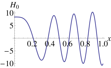
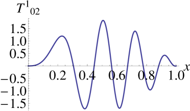
Figure 1: The plots of a solution in the sector $\lambda>0$, in units $\ell=1$,

for $n=0,\mu=100,c_{1}=1,c_{2}=0,\sigma=1$;   left is  $H_{0}$,  right is  $T^{1}{}_{02}(\varphi=0)$.

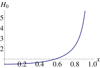
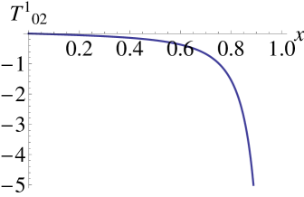
Figure 2: The plots of a solution in the sector $\lambda<0$, in units $\ell=1$,

for $n=0,\mu=\sqrt{8},c_{1}=0.1,c_{2}=0$;   left is  $H_{0}$,  right is  $T^{1}{}_{02}(\varphi=0)$.

In the dS sector (Figure 1), the zero modes of both $H$ and $T^{1}{}_{02}(\varphi=0)$ are regular functions with a clear-cut wave-like behavior in the region $0<x<1$. The plots correspond to the pp_Λ geometry for fixed $u$, and as $u$ increases, the pictures change. In the AdS sector (Figure 2), the solution is singular at $x=1$, or equivalently at $p=0$, and it does not have a typical wave-like shape. For a discussion of the singularity at $p=0$, see Ref. [11]. We also examined a zero mode solution ($n=0$) in the $M_{4}$ sector ($\lambda=0$); its shape is similar to what we have in Figure 2, but it remains finite at $x=1$.

5 Solutions in the spin-$2^{-}$ sector

As we noted at the end of section 3, the spin-$2^{-}$ sector is characterized by $\Theta=0$ and, as a consequence of (1ST), by $Q=0$. Equation (3.8b) for $\Sigma$ reads

$$(\partial_{yy}+\partial_{zz})U-\frac{m^{2}}{p^{2}}U=0\,,$$ (5.1)

where $U=(p/q)\Sigma$ and $m^{2}=m_{2^{-}}^{2}$. Clearly, the solutions for $U$ coincide with the solutions for $V=(p/q)\Theta$ in subsection 4.1. Furthermore, the metric function $H$, defined by $Q=0$, has the GR_Λ form, and the solutions for the torsion functions $K_{\alpha}$ follow from the two equations

$$\partial_{y}U+m^{2}\frac{q}{p}K_{y}=0\,,\qquad\partial_{z}U+m^{2}\frac{q}{p}K_{z}=0\,,$$ (5.2)

the counterparts of those in (4.8).

The fact that the metric of the spin-$2^{-}$ sector is independent of torsion makes this sector, in general, much less interesting. There is, however, one solution in this sector that should be mentioned: it is the solution with $H=0$ for which the metric takes the (A)dS/$M_{4}$ form, and the complete dynamics is carried solely by the torsion. We skip discussing details of this case, as they can be easily reconstructed from the results given in the previous section, following the procedure outlined above.

6 Concluding remarks

In this paper, we found a new family of the exact vacuum solutions of PGT, the family of the pp_Λ waves with torsion. Here, we wish to clarify a few issues that have not been properly covered in the main text.

The essential step in our construction is the ansatz for the RC connection (3.1), which modifies only the radiation piece of the corresponding Riemannian connection (2.3). A characteristic feature of the resulting solution is the presence of the null vector $k^{i}=(0,1,0,0)$ in the spacetime geometry. The vector field $k^{i}\partial_{i}=(p/q)^{2}\partial_{v}$ is orthogonal to the spatial surfaces $u$ = const., and is interpreted as the propagation vector of the pp_Λ wave with torsion. Is such an interpretation justifiable?

Although gravitational waves belong to one of the best known families of exact solutions in GR_Λ, a unique covariant criterion for their precise identification is still missing. One of the early criteria of this type was formulated by Lichnerowicz, based on an analogy with methods used to determine electromagnetic radiation, see Zakharov [7]. This criterion can be formulated as a requirement that the radiation piece of the curvature, $S^{ij}=R^{ij}+\lambda b^{i}b^{j}$, satisfies the radiation conditions:

$$k^{i}S_{ij}=0\,,\qquad\varepsilon^{ijkn}k_{j}S_{kn}=0\,.$$ (6.1a)

However, when applied to a RC geometry, the Lichnerowicz criterion can be naturally extended to include the torsion 2-form:

$$k^{i}T_{i}=0\,,\qquad\varepsilon^{ijmn}k_{m}T_{n}=0\,.$$ (6.1b)

A direct comparison to the expressions (2.4) and (3.2) shows that both sets of the radiation conditions are satisfied. This result gives a strong support to interpreting the pp_Λ waves with torsion as proper wave solutions of PGT.

Looking at the explicit solutions for the pp_Λ waves with torsion, one should note that, in general, the hypergeometric function ${}_{2}F_{1}(a,b,c,x)$ is singular at $x=1$ $(\rho=\ell)$ [19]; moreover, local coordinates we are using are singular at both $x=1$ and $x=0$ (Appendix A). To test the nature of these singularities, we calculated the following torsion and curvature invariants:

$$T^{i}\wedge{{}^{\star}}T_{i}=0\,,$$

$$R=-12\lambda\,,\qquad R^{ij}\wedge{{}^{\star}}R_{i,j}=12\lambda^{2}{\hat{\epsilon}}\,,\qquad R^{ij}{}_{kl}R^{kl}{}_{mn}R^{mn}{}_{ij}=-48\lambda^{3}\,,$$ (6.2)

the fourth order invariant is $96\lambda^{4}$, and so on. All these invariants are well-behaved at $x=1,0$, which might be a signal that the singularities in question are just the coordinate singularities. However, according to Wald [20], the geometric singularities are not always visible in the field strength invariants. Hence, this issue deserves further clarification.

If the curvature $R^{ij}$ is replaced by its radiation piece $S^{ij}$, all the invariants in (6.2) are found to vanish. According to Bell’s second criterion [7], we have here another result that supports the wave interpretation of our pp_Λ solutions.

In conclusion, the family of solutions that we found reveals an unexpected dynamical aspect of torsion. Namely, although torsion is introduced by a minor modification of the Riemannian connection, see (3.1), the metric function $H$ in (4.7) is determined solely by the torsion, and consequently, the form of the metric is a genuine dynamical effect of PGT. A more detailed information could be obtained by analyzing the motion of test particles/fields in the RC spacetimes associated to the pp_Λ waves with torsion.

Appendix A On hyperbolic geometries

(A)dS space can be simply represented as a 4D hyperboloid $H_{4}$ embedded in a 5D Minkowski space $M_{5}$ with metric $\eta_{MN}=(+,-,-,-,\sigma)$,

$$H_{4}:\quad X_{0}^{2}-X_{1}^{2}-X_{2}^{2}-X_{3}^{2}-\sigma X_{5}^{2}=-\sigma\ell^{2}\,,$$ (A.1a)

where $$\sigma=+1 \sigma=-1 H_{4}$$ for a dS space and for an AdS space [9, 21]. The metric on reads

$$ds^{2}=dX_{0}^{2}-dX_{1}^{2}-dX_{2}^{2}-dX_{3}^{2}-\sigma dX_{5}^{2}\,,$$ (A.1b)

and its scalar curvature is $R=-12\sigma/\ell^{2}$. The group of isometries of the dS/AdS spaces is $SO(1,4)/SO(2,3)$, and the corresponding topologies are $R\times S^{3}$ for the dS space, and $S^{1}\times R^{3}$ for the AdS space (or $R^{4}$ for its universal covering).

Going now back to the generalized pp wave metric (2.1), we note that in the limit $H=0$, it describes the background (A)dS geometry:

$$ds^{2}=2\left(\frac{q}{p}\right)^{2}du\left(-2{\mit\Lambda}v^{2}du+dv\right)-\frac{1}{p^{2}}(dy^{2}+dz^{2})\,,$$ (A.2)

$$p=1+{\mit\Lambda}(y^{2}+z^{2}),\qquad q=1-{\mit\Lambda}(y^{2}+z^{2})\,.$$

As we shall see below, ${\mit\Lambda}$ is related to $\ell$ by $4\sigma{\mit\Lambda}=1/\ell^{2}$; moreover, ${\mit\Lambda}>0$ for dS and ${\mit\Lambda}<0$ for AdS. The two forms of the metric associated to the hyperboloid $H_{4}$ are related to each other by a coordinate transformation [11],

$$X_{0}=\frac{q}{2p}(u+v+{\mit\Lambda}u^{2}v)\,,\qquad~{}~{}u=2\sigma\ell\frac{X_{5}-\sqrt{-\sigma(X_{0}^{2}-X_{1}^{2}-\sigma X_{5}^{2})}}{X_{0}-X_{1}}\,,$$

$$X_{1}=\frac{q}{2p}(u-v+{\mit\Lambda}u^{2}v)\,,\qquad~{}~{}v=\frac{X_{0}-X_{1}}{4\ell\sqrt{-\sigma(X_{0}^{2}-X_{1}^{2}-\sigma X_{5}^{2})}}\,,$$

$$X_{2}=\frac{y}{p}\,,\quad X_{3}=\frac{z}{p}\,,\hskip 56.9055pty=\frac{2\ell X_{2}}{\ell+\sqrt{\ell^{2}-\sigma(X_{2}^{2}+X_{3}^{2})}}\,,$$

$$X_{5}=\frac{1}{2\sqrt{\sigma{\mit\Lambda}}}\frac{q}{p}(1+2{\mit\Lambda}uv),\hskip 25.6073ptz=\frac{2\ell X_{3}}{\ell+\sqrt{\ell^{2}-\sigma(X_{2}^{2}+X_{3}^{2})}}\,.$$ (A.3)

Indeed, the coordinates $X_{M}$ in $M_{4}$ describe the hyperboloid $H_{4}$,

$$(X_{0}^{2}-X_{1}^{2}-\sigma X_{5}^{2})-X_{2}^{2}-X_{3}^{2}=-\frac{1}{4{\mit\Lambda}}\frac{q^{2}}{p^{2}}-\frac{1}{p^{2}}(y^{2}+z^{2})=-\frac{1}{4{\mit\Lambda}}=-\sigma\ell^{2}\,,$$

and the corresponding metric (A.1b), followed by the rescaling $v\to 2v$, coincides with (A.2).

Since local coordinates $x^{\mu}=(u,v,x,y)$ are introduced by the parametrization (A.3), they are well defined for

$$X_{0}^{2}-X_{1}^{2}-\sigma X_{5}^{2}=-\frac{1}{4{\mit\Lambda}}\frac{q^{2}}{p^{2}}>0.$$

The limiting value $q=0$ is not allowed, as it represents the singularity of the local coordinate system $(u,v,y,z)$; this singularity is visible only for ${\mit\Lambda}>0$. The same conclusion follows from the fact that the determinant of the metric (A.2) vanishes for $q=0$. Furthermore, an inspection of equations (A.3) reveals the existence of another singularity, located at $p=0$; it is visible only for ${\mit\Lambda}<0$. Thus, local coordinates $(u,v,y,z)$ are restricted to the region where $q$ and/or $p$ do not vanish: $y^{2}+z^{2}\leq|{\mit\Lambda}|^{-1}$. More on the geometric interpretation of these singularities can be found in Ref. [11].

Appendix B Irreducible decomposition of the field strengths

We present here formulas for the irreducible decomposition of the PGT field strengths in a 4D Riemann–Cartan spacetime [4, 22].

The torsion 2-form has three irreducible pieces:

$${}^{(2)}T^{i}=\frac{1}{3}b^{i}\wedge(h_{m}\hbox{\vrule height=0.0pt,width=4.0pt,depth=0.3pt\vrule height=7.0pt,width=0.3pt,depth=0.3pt\vrule height=0.0pt,width=2.0pt,depth=0.0pt}\hskip 0.8ptT^{m})\,,$$

$${}^{(3)}T^{i}=\frac{1}{3}h^{i}\hbox{\vrule height=0.0pt,width=4.0pt,depth=0.3pt\vrule height=7.0pt,width=0.3pt,depth=0.3pt\vrule height=0.0pt,width=2.0pt,depth=0.0pt}\hskip 0.8pt(T^{m}\wedge b_{m})\,,$$

$${}^{(1)}T^{i}=T^{i}-{}^{(2)}T^{i}-{}^{(3)}T^{i}\,.$$ (B.1)

The RC curvature 2-form can be decomposed into six irreducible pieces:

$$\begin{array}[]{ll}{}^{(2)}R^{ij}={}^{*}(b^{[i}\wedge\Psi^{j]})\,,&{}^{(4)}R^{ij}=b^{[i}\wedge\Phi^{j]}\,,\\[3.0pt] {}^{(3)}R^{ij}=\displaystyle\frac{1}{12}X\,{}^{*}(b^{i}\wedge b^{j})\,,&{}^{(6)}R^{ij}=\displaystyle\frac{1}{12}F\,b^{i}\wedge b^{j}\,,\\[9.0pt] {}^{(5)}R^{ij}=\displaystyle\frac{1}{2}b^{[i}\wedge h^{j]}\hbox{\vrule height=0.0pt,width=4.0pt,depth=0.3pt\vrule height=7.0pt,width=0.3pt,depth=0.3pt\vrule height=0.0pt,width=2.0pt,depth=0.0pt}\hskip 0.8pt(b^{m}\wedge F_{m})\,,&{}^{(1)}R^{ij}=R^{ij}-\sum_{a=2}^{6}{}^{(a)}R^{ij}\,.\end{array}$$ (B.2a)

where

$$F^{i}:=h_{m}\hbox{\vrule height=0.0pt,width=4.0pt,depth=0.3pt\vrule height=7.0pt,width=0.3pt,depth=0.3pt\vrule height=0.0pt,width=2.0pt,depth=0.0pt}\hskip 0.8ptR^{mi}={Ric}^{i}\,,\qquad F:=h_{i}\hbox{\vrule height=0.0pt,width=4.0pt,depth=0.3pt\vrule height=7.0pt,width=0.3pt,depth=0.3pt\vrule height=0.0pt,width=2.0pt,depth=0.0pt}\hskip 0.8ptF^{i}=R\,,$$

$$X^{i}:={}^{*}(R^{ik}\wedge b_{k})\,,\qquad X:=h_{i}\hbox{\vrule height=0.0pt,width=4.0pt,depth=0.3pt\vrule height=7.0pt,width=0.3pt,depth=0.3pt\vrule height=0.0pt,width=2.0pt,depth=0.0pt}\hskip 0.8ptX^{i}\,.$$ (B.2b)

and

$$\Phi_{i}:=F_{i}-\frac{1}{4}b_{i}F-\frac{1}{2}h_{i}\hbox{\vrule height=0.0pt,width=4.0pt,depth=0.3pt\vrule height=7.0pt,width=0.3pt,depth=0.3pt\vrule height=0.0pt,width=2.0pt,depth=0.0pt}\hskip 0.8pt(b^{m}\wedge F_{m})\,,$$

$$\Psi_{i}:=X_{i}-\frac{1}{4}b_{i}X-\frac{1}{2}h_{i}\hbox{\vrule height=0.0pt,width=4.0pt,depth=0.3pt\vrule height=7.0pt,width=0.3pt,depth=0.3pt\vrule height=0.0pt,width=2.0pt,depth=0.0pt}\hskip 0.8pt(b^{m}\wedge X_{m})\,.$$ (B.2c)

The above formulas differ from those in Refs. [4, 22] in two minor details: the definitions of $F^{i}$ and $X^{i}$ are taken with an additional minus sign, but at the same time, the overall signs of all the irreducible curvature parts are also changed, leaving their final content unchanged.

Appendix C Calculating the PGT field equations

The gravitational dynamics of PGT is determined by a Lagrangian $L_{G}=L_{G}(b^{i},T^{i},R^{ij})$ (4-form), which is assumed to be at most quadratic in the field strengths (quadratic PGT) and parity invariant [23]. The form of $L_{G}$ can be conveniently represented as

$$L_{G}=-{{}^{\star}}(a_{0}R+2{\mit\Lambda})+\frac{1}{2}T^{i}H_{i}+\frac{1}{4}R^{ij}H^{\prime}_{ij}\,,$$ (C.1)

where $H_{i}:=\partial L_{G}/\partial T^{i}$ (the covariant momentum) and $H^{\prime}_{ij}$ define the quadratic terms in $L_{G}$:

$$H_{i}=2\sum_{n=1}^{3}{{}^{\star}}(a_{n}{}^{(n)}T_{i})\,,\qquad H^{\prime}_{ij}:=2\sum_{n=1}^{6}{{}^{\star}}(b_{n}{}^{(n)}R_{ij})\,.$$ (C.2a)

Varying $$L_{G} b^{i} \omega^{ij} H_{ij}:=\partial L_{G}/\partial R^{ij}$$ with respect to and yields the PGT field equations in vacuum. After introducing the complete covariant momentum by

$$H_{ij}=-2a_{0}{{}^{\star}}(b^{i}b^{j})+H^{\prime}_{ij}\,,$$ (C.2b)

these equations can be written in a compact form as [4, 22]

$$(1ST) \nabla H_{i}+E_{i}=0\,,$$

$$(2ND) \nabla H_{ij}+E_{ij}=0\,,$$ (C.3)

where $E_{i}$ and $E_{ij}$ are the gravitational energy-momentum and spin currents:

$$E_{i}:=h_{i}\hbox{\vrule height=0.0pt,width=4.0pt,depth=0.3pt\vrule height=7.0pt,width=0.3pt,depth=0.3pt\vrule height=0.0pt,width=2.0pt,depth=0.0pt}\hskip 0.8ptL_{G}-(h_{i}\hbox{\vrule height=0.0pt,width=4.0pt,depth=0.3pt\vrule height=7.0pt,width=0.3pt,depth=0.3pt\vrule height=0.0pt,width=2.0pt,depth=0.0pt}\hskip 0.8ptT^{m})H_{m}-\frac{1}{2}(h_{i}\hbox{\vrule height=0.0pt,width=4.0pt,depth=0.3pt\vrule height=7.0pt,width=0.3pt,depth=0.3pt\vrule height=0.0pt,width=2.0pt,depth=0.0pt}\hskip 0.8ptR^{mn})H_{mn}\,,$$

$$E_{ij}:=-(b_{i}H_{j}-b_{j}H_{i})\,.$$ (C.4)

The above procedure is used in subsection 3.2 to find explicit form of the PGT field equations for the pp_Λ waves with torsion, with the result displayed in Eqs. (3.6), (3.7) and (3.8). To simplify calculation of the term $\nabla{{}^{\star}}{}^{(1)}R_{ij}$ in $\nabla H_{ij}$, we used the identity

$$\frac{1}{2}\nabla{{}^{\star}}R_{ij}=\nabla{{}^{\star}}{}^{(2)}R_{ij}+\nabla{{}^{\star}}{}^{(4)}R_{ij}\,,$$ (C.5)

that follows from the Bianchi identity $\nabla R^{ij}=0$ and the double duality properties of the irreducible parts of the curvature.

References

- [1] H. Weyl, Electron and gravitation, I. (in German), Zeitschrift für Physik, 56 (1929) 330–352, translated in: L. O Raifeartaigh, The Dawning of Gauge Theory (Princeton University Press, Princeton, 1997), pp. 121–144.
- [2] T. W. B. Kibble, Lorentz invariance and the gravitational field, J. Math. Phys. 2, 212–221 (1961); D. W. Sciama, On the analogy between charge and spin in general relativity, in: Recent Developments in General Relativity, Festschrift for Infeld (Pergamon Press, Oxford; PWN, Warsaw, 1962) pp. 415–439.
- [3] M. Blagojević, Gravitation and Gauge Symmetries (IoP Publishing, Bristol, 2002); T. Ortýn, Gravity and Strings (Cambridge University Press, Cambridge, 2004).
- [4] Yu. N. Obukhov, Poincaré gauge gravity: Selected topics, Int. J. Geom. Meth. Mod. Phys. 3, 95–138 (2006).
- [5] M. Blagojević and F. W. Hehl (eds.), Gauge Theories of Gravitation, A Reader with Commentaries (Imperial College Press, London, 2013).
- [6] J. Ehlers and W. Kundt, Exact solutions of the gravitational field equations, in: Gravitation: an Introduction to Current Research, ed. L. Witten (Willey, New York, 1962) pp. 49–101.
- [7] V. Zakharov, Gravitational Waves in Einstein’s Theory (Halsted Press, New York, 1973).
- [8] H. Stephani, D. Kramer, M. MacCallum, C. Hoenselaers, and E. Herlt, Exact Solutions to Einstein s Field Equations, 2nd ed. (Cambridge University Press, Cambridge, 2003).
- [9] J. B. Griffiths and J. Podolský, Exact Space-Times in Einstein’s General Relativity, (Cambridge University Press, Cambridge, 2009).
- [10] J. Bičák and J. Podolský, Gravitational waves in vacuum spacetimes with cosmological constant: I. Classification and geometrical properties of nontwisting type N solutions, J. Math. Phys. 40, 4495–4505 (1999).
- [11] J. B. Griffiths, P. Docherty and J. Podolský, Generalized Kundt waves and their physical interpretation, Class. Quant. Grav. 21, 207–222 (2004).
- [12] I. Osváth, I. Robinson and K. Rózga, Plane-fronted gravitational and electromagnetic waves in spaces with cosmological constant, J. Math. Phys. 26, 1755-1761 (1985).
- [13] M. Blagojević and B. Cvetković, Siklos waves in Poincaré gauge theory, Phys. Rev. D 93 (2016) 044018 (9 pages); see also: Siklos waves with torsion in 3D, JHEP 11, 141 (2014) [16 pages].
- [14] W. Adamowicz, Plane waves in gauge theories of gravitation, Gen. Rel. Grav. 12, 677–691 (1980); M.-K. Chen, D.-C. Chern, R.-R. Hsu, and W. B. Yeung, Plane-fronted torsion waves in a gravitational gauge theory with a quadratic Lagrangian, Phys. Rev. D 28, 2094–2095 (1983); R. Sippel and H. Goenner, Symmetry classes of pp-waves, Gen. Rel. Grav. 18, 1229–1243 (1986); P. Singh, On null tratorial torsion in vacuum quadratic Poincaré gauge theory, Class. Quant. Grav. 7, 2125–2130 (1990); P. Singh and J. B. Griffiths, A new class of exact solutions of the vacuum quadratic Poincare gauge field theory, Gen. Rel. Grav. 22, 947–956 (1990); V. V. Zhytnikov, Wavelike exact solutions of gravity, J. Math. Phys. 35, 6001–6017 (1994); O. V. Babourova, B. N. Frolov and E. A. Klimova, Plane torsion waves in quadratic gravitational theories, Class. Quant. Grav. 16, 1149–1162 (1999); A. D. King and D. Vassiliev, Torsion waves in metric-affine field theory, Class. Quantum Grav. 18, 2317–2329 (2001); V. Pasic and D. Vassiliev, PP-waves with torsion and metric-affine gravity, Class. Quant. Grav. 22, 3961–3976 (2005). V. Pasic and E. Barakovic, PP-waves with torsion: a metric-affine model for the massless neutrino, Gen. Rel. Grav. 46, 1787 (2014) [27 pages].
- [15] Yu. N. Obukhov, Generalized plane-fronted gravitational waves in any dimension, Phys. Rev. D 69, 024013 (2004).
- [16] The field equations (3.6) for the ppΛ waves with torsion are checked using the Excalc package of the computer algebra system Reduce; after being transformed to the form (3.8), they are solved with the help of Wolfram Mathematica.
- [17] K. Hayashi and T. Shirafuji, Gravity from Poincaré gauge theory of fundamental interactions. I, General formulation, Prog. Theor. Phys. 64, 866–882 (1980); IV, Mass and energy of particle spectrum, Prog. Theor. Phys. 64, 2222–2241 (1980).
- [18] E. Sezgin and P. van Nieuwenhuizen, New ghost-free gravity Lagrangians with propagating torsion, Phys. Rev. 21, 3269–3280 (1980); E. Sezgin, Class of ghost-free gravity Lagrangians with massive or massless propagating modes, Phys. Rev. 24, 1677–1680 (1981).
- [19] G. E. Andrews, R. Askey, and R. Roy, Special functions (Cambridge University Press, Cambridge, 1999); Z. X. Wang and D. R. Guo, Special Functions (World Scientific, Singapore, 1989).
- [20] R. M. Wald, General Relativity (The University of Chicago Press, Chicago, 1984).
- [21] S. W. Hawking and G. F. R. Ellis, The large Scale Structure of Spacetime (Cambridge University Press, 1973).
- [22] F. W. Hehl, J. D. McCrea, E. W. Mielke, and Y. Neeman, Metric-affine gauge theory of gravity: Field equations, Noether identities, world spinors, and breaking of dilation invariance, Phys. Rept. 258, 1–171 (1995).
- [23] Y. N. Obukhov, Gravitational waves in Poincar]é gauge gravity theory, unpublished work (February 2017). The author studies the plane-fronted gravitational waves using the most general quadratic PGT Lagrangian with both parity even and parity odd terms, but assuming .