Large deformations of the Tracy-Widom distribution I. Non-oscillatory asymptotics

Abstract.

We analyze the left-tail asymptotics of deformed Tracy-Widom distribution functions describing the fluctuations of the largest eigenvalue in invariant random matrix ensembles after removing each soft edge eigenvalue independently with probability $1-\gamma\in[0,1]$. As $\gamma$ varies, a transition from Tracy-Widom statistics ($\gamma=1$) to classical Weibull statistics ($\gamma=0$) was observed in the physics literature by Bohigas, de Carvalho, and Pato [12]. We provide a description of this transition by rigorously computing the leading-order left-tail asymptotics of the thinned GOE, GUE and GSE Tracy-Widom distributions. In this paper, we obtain the asymptotic behavior in the non-oscillatory region with $\gamma\in[0,1)$ fixed (for the GOE, GUE, and GSE distributions) and $\gamma\uparrow 1$ at a controlled rate (for the GUE distribution). This is the first step in an ongoing program to completely describe the transition between Tracy-Widom and Weibull statistics. As a corollary to our results, we obtain a new total-integral formula involving the Ablowitz-Segur solution to the second Painlevé equation.

1. Introduction

The Tracy-Widom distribution functions $F_{\beta}$ are universal probability distributions describing extremal behavior of, among a host of other applications, eigenvalues in the Gaussian invariant ensembles [46, 47], the increasing subsequences of a random permutation [5], last-passage percolation, randomly growing Young diagrams, and vicious random walkers [41, 7], the KPZ growth model [44], and growing interfaces in liquid crystals [45]. Specifically, consider the three classical random matrix ensembles GOE ($\beta=1$), GUE ($\beta=2$) and GSE ($\beta=4$), i.e. we choose a Hermitian matrix X with real ($\beta=1$), complex ($\beta=2$), or real quaternion ($\beta=4$) entries and underlying eigenvalue probability density function of the form

$$\frac{1}{Z_{N,\beta}}\prod_{1\leq j<k\leq N}|\lambda_{k}-\lambda_{j}|^{\beta}\exp\left(-\frac{\beta}{2}\sum_{j=1}^{N}\lambda_{j}^{2}\right)$$

with a normalization constant $Z_{N,\beta}$. The Tracy-Widom functions $F_{\beta}(s)$ are the distribution functions of the (properly centered and scaled) largest eigenvalue $\lambda_{\max}({\bf X})$ as the matrix size $N$ tends to infinity:

$$\lim_{N\rightarrow\infty}\mathbb{P}\left(\frac{\lambda_{\max}({\bf X})-\sqrt{2N}}{2^{-\frac{1}{2}}N^{-\frac{1}{6}}}\leq s\right)=F_{\beta}(s),\ \ s\in\mathbb{R},\ \ \ \ \beta=1,2,4.$$ (1.1)

Quite remarkably, the three distribution functions admit the representations [46, 47]

$$F_{2}(s)=\exp\left(-\int_{s}^{\infty}(t-s)u_{{}_{\textnormal{HM}}}^{2}(t)\,{\mathrm{d}}t\right),\ \ \ \big{(}F_{1}(s)\big{)}^{2}=F_{2}(s)\mathrm{e}^{-\mu(s)},\ \ \ \big{(}F_{4}(s)\big{)}^{2}=F_{2}(s)\cosh^{2}\left(\frac{1}{2}\mu(s)\right)$$

in terms of the Hastings-McLeod [37] solution $u_{{}_{\textnormal{HM}}}=u_{{}_{\textnormal{HM}}}(x)$ to the Painlevé-II equation

$$u^{\prime\prime}_{{}_{\textnormal{HM}}}=xu_{{}_{\textnormal{HM}}}+2u^{3}_{{}_{\textnormal{HM}}},\ \ \ \ \ (^{\prime})=\frac{{\mathrm{d}}}{{\mathrm{d}}x};\ \ \ \ \ \ \ u_{{}_{\textnormal{HM}}}(x)=\frac{x^{-\frac{1}{4}}}{2\sqrt{\pi}}\mathrm{e}^{-\frac{2}{3}x^{\frac{3}{2}}}\big{(}1+o(1)\big{)},\ \ x\rightarrow+\infty$$

and its antiderivative

$$\mu(s):=\int_{s}^{\infty}u_{{}_{\textnormal{HM}}}(t)\,{\mathrm{d}}t.$$

The distribution functions $F_{\beta}(s)$ are central to modern integrable probability but they are very different from the classical normal distribution; in particular we note that

$$F_{\beta}(s)=1-c_{\beta}s^{-\frac{3\beta}{4}}\mathrm{e}^{-\frac{2\beta}{3}s^{\frac{3}{2}}}\big{(}1+o(1)\big{)},\ \ \ s\rightarrow+\infty;\ \ \ \ c_{1}=\frac{1}{4\sqrt{\pi}},\ c_{2}=\frac{1}{16\pi},\ c_{4}=\frac{1}{512\pi},$$

and [46, 26, 3, 4, 16], as $s\rightarrow-\infty$,

$$F_{1}(s)= \,\,\tau_{1}(-s)^{-\frac{1}{16}}\mathrm{e}^{\frac{1}{24}s^{3}-\frac{1}{3\sqrt{2}}(-s)^{\frac{3}{2}}}\big{(}1+o(1)\big{)},\ \ \ \ \ \ F_{2}(s)=\tau_{2}(-s)^{-\frac{1}{8}}\mathrm{e}^{\frac{1}{12}s^{3}}\big{(}1+o(1)\big{)},$$ (1.2)

$$F_{4}(s)= \,\,\tau_{4}(-s)^{-\frac{1}{16}}\mathrm{e}^{\frac{1}{24}s^{3}+\frac{1}{3\sqrt{2}}(-s)^{\frac{3}{2}}}\big{(}1+o(1)\big{)};\ \ \ \ \tau_{1}=2^{-\frac{11}{48}}\mathrm{e}^{\frac{1}{2}\zeta^{\prime}(-1)},\tau_{2}=2^{\frac{1}{24}}\mathrm{e}^{\zeta^{\prime}(-1)},\ \tau_{4}=2^{-\frac{35}{48}}\mathrm{e}^{\frac{1}{2}\zeta^{\prime}(-1)}$$

in terms of the Riemann-zeta function $\zeta(z)$. Our focus lies on the distribution of the largest eigenvalue $\lambda_{\max}({\bf X},\gamma)$ in the following thinned process: let $\lambda_{1}({\bf X})<\ldots<\lambda_{\max}({\bf X})$ denote the eigenvalues of a GOE, GUE, or GSE matrix ${\bf X}$ and fix a number $\gamma\in[0,1]$. Now, discard each eigenvalue independently with probability $1-\gamma$ and define $\lambda_{\max}({\bf X},\gamma)$ as the largest observed eigenvalue after thinning. In the large-$N$ limit its distribution function leads to a one-parameter generalization of (1.1):

$$F_{\beta}(s,\gamma):=\lim_{N\rightarrow\infty}\mathbb{P}\left(\frac{\lambda_{\max}({\bf X},\gamma)-\sqrt{2N}}{2^{-\frac{1}{2}}N^{-\frac{1}{6}}}\leq s\right),\ \ \ \ \ s\in\mathbb{R},\ \ \ \beta=1,2,4.$$ (1.3)

This again admits a Painlevé representation, as proven in Subsection 1.2 below.

Proposition 1.1.

Let $u_{{}_{\textnormal{AS}}}=u_{{}_{\textnormal{AS}}}(x,\gamma)$ denote the Ablowitz-Segur [1] solution to the Painlevé-II equation

$$u^{\prime\prime}_{{}_{\textnormal{AS}}}=xu_{{}_{\textnormal{AS}}}+2u^{3}_{{}_{\textnormal{AS}}},\ \ \ \ \ (^{\prime})=\frac{{\mathrm{d}}}{{\mathrm{d}}x};\ \ \ \ \ \ \ u_{{}_{\textnormal{AS}}}(x,\gamma)=\sqrt{\gamma}\,\frac{x^{-\frac{1}{4}}}{2\sqrt{\pi}}\mathrm{e}^{-\frac{2}{3}x^{\frac{3}{2}}}\big{(}1+o(1)\big{)},\ \ x\rightarrow+\infty.$$ (1.4)

For any $s\in\mathbb{R}$ and $\gamma\in[0,1]$, the deformed Tracy-Widom distribution functions (1.3) equal

$$F_{2}(s,\gamma)=\exp\left(-\int_{s}^{\infty}(t-s)u_{{}_{\textnormal{AS}}}^{2}(t,\gamma)\,{\mathrm{d}}t\right),\ \ \ \ \big{(}F_{4}(s,\gamma)\big{)}^{2}=F_{2}(s,\gamma)\cosh^{2}\left(\frac{1}{2}\mu(s,\gamma)\right),$$ (1.5)

and

$$\big{(}F_{1}(s,\gamma)\big{)}^{2}=F_{2}(s,\overline{\gamma})\frac{\gamma-1-\cosh\mu(s,\overline{\gamma})+\sqrt{\overline{\gamma}}\sinh\mu(s,\overline{\gamma})}{\gamma-2},\ \ \ \overline{\gamma}:=2\gamma-\gamma^{2}\in[0,1],$$ (1.6)

where

$$\mu(s,\gamma):=\int_{s}^{\infty}u_{{}_{\textnormal{AS}}}(t,\gamma)\,{\mathrm{d}}t.$$ (1.7)

The thinning operation is well known in the theory of point processes, see e.g. [40], but was studied in a random matrix theory context only recently by Bohigas and Pato [13, 14] and later by Bohigas, de Carvalho, and Pato [12]. Their motivation was a fundamental question in nuclear physics: how can one recover a missing energy level (i.e. eigenvalue) from an otherwise complete set of measurements? As observed by Dyson, if the energy levels are completely correlated (such as evenly spaced levels, also referred to as picket fence statistics), then missing levels can be easily identified, while if there is no correlation (Poisson statistics), there is no possibility of finding the missing level. The scattering resonances of neutrons scattered off a heavy nucleus are known to obey random matrix eigenvalue statistics, which lie in an intermediate correlation regime. The thinning process reduces the amount of level repulsion (a correlating effect), so the thinned Gaussian ensembles interpolate between moderate correlations when $\gamma=1$ (random matrix statistics) and no correlations when $\gamma=0$ (classical extreme value statistics). The extreme value theorem states that the limiting distribution of the maximum of a sequence of independent identically distributed random variables must be a Gumbel (type I), Fréchet (type II), or Weibull (type III) distribution, provided the limit exists. Since GOE, GUE, and GSE eigenvalues obey the semicircle law [34], i.e. we have the following weak convergence for the empirical measure:

$$\frac{1}{N}\sum_{j=1}^{N}\delta_{\lambda_{j}({\bf X})}(y)\rightharpoonup\frac{1}{\pi}\sqrt{2N-y^{2}}\,\chi_{(-\sqrt{2N},\sqrt{2N})}(y),\ \ \ \chi_{A}(y)=\begin{cases}1,&y\in A\\ 0,&y\notin A,\end{cases}$$

it is reasonable to expect type III behavior in the $\gamma=0$ limit. Indeed, following the approach of Bohigas, de Carvalho, and Pato [12], we first note that (1.1) is equivalent to a gap probability for the rescaled eigenvalues $\mu_{j}({\bf X}):=2^{\frac{1}{2}}N^{\frac{1}{6}}(\lambda_{j}({\bf X})-\sqrt{2N})$, i.e.

$$F_{\beta}(s)=\lim_{N\rightarrow\infty}\mathbb{P}\big{(}\#\{j:\ \mu_{j}({\bf X})\in(s,\infty)\}=0\big{)}.$$

But once we thin out the soft-edge scaled eigenvalues $\mu_{j}({\bf X})$ the average number of eigenvalues in the interval $(s,\infty)$ is reduced, so we want to scale $s$ with $\gamma$ accordingly in order to keep the level density of the remaining fraction $\gamma$ constant. In order to find the correct scale we note that, as $N\rightarrow\infty$, to leading order

$$N=\frac{1}{\pi}\int_{-\sqrt{2N}}^{\sqrt{2N}}\sqrt{2N-y^{2}}\,{\mathrm{d}}y\sim\frac{1}{\pi}\int_{-4N^{\frac{2}{3}}}^{0}\sqrt{-\mu}\,{\mathrm{d}}\mu,\ \$$

so the average number of eigenvalues in $(s,\infty)$ equals

$$\frac{1}{\pi}\int_{s}^{\infty}\sqrt{-\mu}\,\chi_{(-\infty,0)}(\mu)\,{\mathrm{d}}\mu=\frac{2}{3\pi}(-s)^{\frac{3}{2}},\ s<0,$$

i.e. we should replace $s$ in (1.3) by $\gamma^{-\frac{2}{3}}s$ in order to keep it invariant. Now, return to (1.3) and use (1.4) and (1.5) to see

$$F_{\beta}(s,\gamma)=1-c_{\beta}\gamma^{\frac{\beta}{2}}s^{-\frac{3\beta}{4}}\mathrm{e}^{-\frac{2\beta}{3}s^{\frac{3}{2}}}\big{(}1+o(1)\big{)},\ \ \ s\rightarrow+\infty,$$

which holds uniformly for $\gamma\in[0,1]$. Thus,

$$\lim_{\gamma\downarrow 0}F_{\beta}\big{(}\gamma^{-\frac{2}{3}}s,\gamma\big{)}=1,\ \ s>0.$$ (1.8)

The left ($s\rightarrow-\infty$) tail behavior of $F_{\beta}(s,\gamma)$ is more subtle, and it is here where the derivation in [12] becomes non-rigorous: combine

$$\frac{\partial}{\partial s}\ln F_{2}(s,\gamma)=\int_{s}^{\infty}u^{2}_{{}_{\textnormal{AS}}}(x,\gamma)\,{\mathrm{d}}x=\big{(}u_{{}_{\textnormal{AS}}}^{\prime}(s,\gamma)\big{)}^{2}-su_{{}_{\textnormal{AS}}}^{2}(s,\gamma)-u_{{}_{\textnormal{AS}}}^{4}(s,\gamma)$$

with the known asymptotic expansion [1, 2]

$$u_{{}_{\textnormal{AS}}}(x,\gamma)=(-x)^{-\frac{1}{4}}\sqrt{\frac{v}{\pi}}\cos\left(\frac{2}{3}(-x)^{\frac{3}{2}}-\frac{v}{2\pi}\ln\big{(}8(-x)^{\frac{3}{2}}\big{)}+\phi\right)+\mathcal{O}\left((-x)^{-1}\right),\ \ x\rightarrow-\infty,$$

valid for fixed $v=-\ln(1-\gamma)\in[0,\infty)$ where $\phi=\frac{\pi}{4}-\textnormal{arg}\,\Gamma(\frac{v}{2\pi\mathrm{i}})$. Thus, back in (1.5) and (1.6) we have

$$F_{\beta}(s,\gamma)=\tau_{\beta}(\gamma)(-s)^{\frac{3v^{2}}{4\beta\pi^{2}}}\exp\left(-vg_{\beta}(-s)^{\frac{3}{2}}\right)\big{(}1+o(1)\big{)},\ \ s\rightarrow-\infty;\ \ \ \ g_{1}=g_{2}=\frac{2}{3\pi},\ \ g_{4}=\frac{1}{3\pi}$$ (1.9)

with undetermined integration constants $\tau_{\beta}(\gamma)$. Ignoring these constant factors and all error terms we then find from (1.9), together with (1.8),

$$\lim_{\gamma\downarrow 0}F_{\beta}\big{(}\gamma^{-\frac{2}{3}}s,\gamma\big{)}=\begin{cases}\exp\left(-g_{\beta}(-s)^{\frac{3}{2}}\right),&s\leq 0\\ 1,&s>0,\end{cases}$$ (1.10)

which is a simple transformation of the Weibull distribution function with scale parameter $g_{\beta}$ and Weibull slope $\frac{3}{2}$, see Figure 1 below.

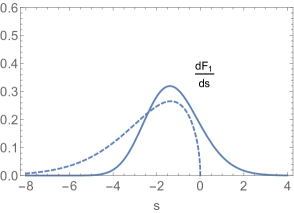
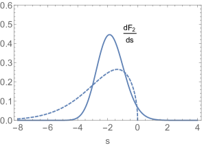
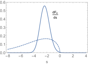
Figure 1. The three Tracy-Widom densities $\frac{{\mathrm{d}}F_{\beta}}{{\mathrm{d}}s}$ as solid lines for $\beta=1,2,4$ from left to right. The dashed lines are the corresponding limiting Weibull densities from (1.10).

We can confirm (1.10) rigorously using Theorems 1.2 and 1.3 below which are the main results of the paper.

1.1. Statement of results and discussion

Theorem 1.2.

For any fixed $0<\epsilon<\frac{1}{2}$, there exist constants $s_{0}=s_{0}(\epsilon)>0$ and $c_{j}=c_{j}(\epsilon)>0$, $j=1,2$, so that

$$\ln F_{2}(s,\gamma)=-\frac{2v}{3\pi}(-s)^{\frac{3}{2}}+\frac{v^{2}}{4\pi^{2}}\ln\big{(}8(-s)^{\frac{3}{2}}\big{)}+\ln\left(G\Big{(}1+\frac{\mathrm{i}v}{2\pi}\Big{)}G\Big{(}1-\frac{\mathrm{i}v}{2\pi}\Big{)}\right)+r_{2}(s,v)$$ (1.11)

for $-s\geq s_{0}$ and $0\leq v=-\ln(1-\gamma)<(-s)^{\frac{1}{2}-\epsilon}$. Here $G(z)$ is the Barnes $G$-function (see [43]), the error term $r_{2}(s,v)$ is differentiable with respect to $s$, and we have

$$\big{|}r_{2}(s,v)\big{|}\leq c_{1}\frac{v^{3}}{|s|^{\frac{3}{2}}}+c_{2}\frac{v}{|s|}\ \ \ \ \ \forall\,(-s)\geq s_{0},\ \ 0\leq v<(-s)^{\frac{1}{2}-\epsilon}.$$

Theorem 1.3.

For any fixed $\gamma\in[0,1)$, there exist positive constants $s_{0}=s_{0}(v)$ and $c_{j}=c_{j}(v)$ such that

$$\ln F_{1}(s,\gamma)=-\frac{2v}{3\pi}(-s)^{\frac{3}{2}}+\frac{v^{2}}{2\pi^{2}}\ln\big{(}8(-s)^{\frac{3}{2}}\big{)}+\frac{1}{2}\ln\left(G\left(1+\frac{\mathrm{i}v}{\pi}\right)G\left(1-\frac{\mathrm{i}v}{\pi}\right)\right)+\frac{1}{2}\ln\left(\frac{2}{1+\mathrm{e}^{v}}\right)+r_{1}(s,v)$$

and

$$\ln F_{4}(s,\gamma)= \,-\frac{v}{3\pi}(-s)^{\frac{3}{2}}+\frac{v^{2}}{8\pi^{2}}\ln\big{(}8(-s)^{\frac{3}{2}}\big{)}+\frac{1}{2}\ln\left(G\left(1+\frac{\mathrm{i}v}{2\pi}\right)G\left(1-\frac{\mathrm{i}v}{2\pi}\right)\right)$$

$$+\ln\left(\frac{1}{2}\left(\frac{1+\sqrt{1-\mathrm{e}^{-v}}}{1-\sqrt{1-\mathrm{e}^{-v}}}\right)^{\frac{1}{4}}+\frac{1}{2}\left(\frac{1-\sqrt{1-\mathrm{e}^{-v}}}{1+\sqrt{1-\mathrm{e}^{-v}}}\right)^{\frac{1}{4}}\right)+r_{4}(s,v)$$

for $-s\geq s_{0}$ and $0\leq v=-\ln(1-\gamma)<+\infty$. The function $G(z)$ is again the Barnes G-function, the error terms $r_{1}(s,v)$ and $r_{4}(s,v)$ are differentiable with respect to $s$, and

$$\big{|}r_{j}(s,v)\big{|}\leq\frac{c_{j}(v)}{|s|^{\frac{3}{4}}}\ \ \ \ \ \forall\,(-s)\geq s_{0},\ \ \ j=1,4.$$

While the results of Theorem 1.2 and 1.3 settle the deformation from Tracy-Widom $F_{1}$, $F_{2}$, and $F_{4}$ statistics ($\gamma=1$) to classical Weibull statistics (1.10) ($\gamma=0$) rigorously, they do not capture the full transition regime! In fact, comparing (1.10) to (1.2) we might ask the important question:

How is the exponential decay $\exp(-vg_{\beta}(-s)^{\frac{3}{2}})$ in (1.9) changed to the super-exponential decay $\exp(s^{3}/24)$ or $\exp(s^{3}/12)$ in (1.2) as $\gamma\uparrow 1$, or equivalently as $v=-\ln(1-\gamma)\rightarrow+\infty$?

This question is the central reason behind the growth condition placed on $v$ in (1.11). As long as $v$ does not grow faster as $(-s)^{\frac{1}{2}-\epsilon}$, all leading terms in the left-tail GUE expansion are unchanged from $v\in[0,+\infty)$ fixed, i.e. we are dealing with quasi-Weibull tails. On the other hand, we have

Theorem 1.4 ([18], Theorem $1.4$).

Given $\chi\in\mathbb{R}$, let $p=p(\chi)\in\mathbb{Z}_{\geq 0}$ be such that $p=0$ for $\chi<-\frac{1}{2}$ and $\chi+\frac{1}{2}<p\leq\chi+\frac{3}{2}$ for $\chi\geq-\frac{1}{2}$. Then, as $s\rightarrow-\infty$,

$$\ln F_{2}(s,\gamma)=\frac{s^{3}}{12}-\frac{1}{4}\ln(-s)+\ln\tau_{2}+\sum_{j=0}^{p-1}\ln\left(1+\frac{j!}{\sqrt{\pi}}2^{-\frac{7}{2}j-\frac{9}{4}}(-s)^{-\frac{3}{2}j-\frac{3}{4}}\mathrm{e}^{\frac{2}{3}\sqrt{2}(-s)^{\frac{3}{2}}-v}\right)+o(1),$$ (1.12)

which holds uniformly for $v\geq\frac{2}{3}\sqrt{2}\,(-s)^{\frac{3}{2}}-\chi\ln\big{(}(-s)^{\frac{3}{2}}\big{)}$.

So, once $v$ grows at least as fast as $\frac{2}{3}\sqrt{2}(-s)^{\frac{3}{2}}$, we observe already Tracy-Widom tails. Combining (1.11) and (1.12), we, thus far, only have an answer to our question for the GUE in the disjoint regions

$$(t,v)\in\mathbb{R}^{2}:\ \ \ t=(-s)^{\frac{3}{2}}\geq t_{0},\ \ \ \ \ \ \varkappa:=\frac{v}{t}\in\left[0,t^{-\frac{1}{3}-\frac{2}{3}\epsilon}\right)\bigsqcup\left[\frac{2}{3}\sqrt{2}-\chi\frac{\ln t}{t},+\infty\right].$$

See Figure 2 below. These regions form the non-oscillatory part of the transition asymptotics of $F_{2}(s,\gamma)$ as $s\rightarrow-\infty$. Our next step is the analysis in the outstanding parameter domain which is ongoing work [19] for the thinned GOE/GUE and GSE Tracy-Widom distributions. There, for faster growing $\gamma$, the Riemann-Hilbert analysis carried out below changes significantly and requires the use of elliptic functions. These elliptic functions degenerate at both ends ($\varkappa\downarrow 0$ and $\varkappa\uparrow\frac{2}{3}\sqrt{2}$) and oscillations vanish: at one end ($\varkappa\downarrow 0$) oscillations die out via decreasing amplitudes and fixed periods, at the other end ($\varkappa\uparrow\frac{2}{3}\sqrt{2}$) via fixed amplitudes and increasing periods.

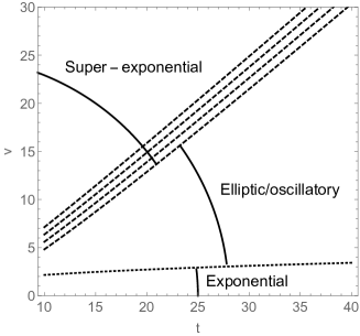
Figure 2. Left-tail behavior of $F_{2}(s,\gamma)$ as $s\to-\infty$, $\gamma\to 1$ in terms of $v=-\ln(1-\gamma)$ and $t=(-s)^{\frac{3}{2}}$. This work determines the asymptotics in the exponential region (see Theorem 1.2). For the super-exponential region see Equation (1.2). Dotted line: $v=t^{\frac{1}{3}}$. Dashed lines: $v=\frac{2}{3}\sqrt{2}t-\chi\ln t$ for various values of $\chi$.

Remark 1.5.

We emphasize that the appearance of an oscillatory intermediate regime in the left tail expansion of $F_{\beta}(s,\gamma)$ was first observed numerically in the paper by Bohigas, de Carvalho and Pato [12]. The similarity between $F_{2}(s)$ and $F_{2}(s,\gamma)$ with $\gamma\neq 1$ in (1.5) suggests an (alternate) approach to understanding these oscillations by analyzing the transition between $u_{{}_{\textnormal{AS}}}(x,\gamma)$ and $u_{{}_{\textnormal{HM}}}(x)$ as $\gamma\uparrow 1$. See [17] for recent progress on this front.

At this point we reformulate the result of Theorem 1.2 in terms of the underlying Painlevé transcendent (1.4), which leads us to the following total integral formula.

Corollary 1.6.

Let $u_{{}_{\textnormal{AS}}}(x,\gamma)$ denote the Ablowitz-Segur Painlevé-II solution as defined in (1.4). Then, for any fixed $\gamma\in[0,1)$,

$$\lim_{s\rightarrow-\infty}\left(-\int_{s}^{\infty}(t-s)u_{{}_{\textnormal{AS}}}^{2}(t,\gamma)\,{\mathrm{d}}t+\frac{2v}{3\pi}(-s)^{\frac{3}{2}}-\frac{3v^{2}}{8\pi^{2}}\ln(-s)\right)=\frac{3v^{2}}{4\pi^{2}}\ln 2+\ln\left(G\Big{(}1+\frac{\mathrm{i}v}{2\pi}\Big{)}G\Big{(}1-\frac{\mathrm{i}v}{2\pi}\Big{)}\right).$$

Remark 1.7.

In recent work computing asymptotics of orthogonal polynomials with a discontinuous Gaussian weight, Bogatskiy, Claeys, and Its [11] in fact conjectured the above total integral, or equivalently the thinned GUE constant factor

$$\ln\tau_{2}(\gamma)=\frac{3v^{2}}{4\pi^{2}}\ln 2+\ln\left(G\left(1+\frac{iv}{2\pi}\right)G\left(1-\frac{iv}{2\pi}\right)\right)$$

in (1.9) for any fixed $\gamma\in\mathbb{C}\backslash[1,+\infty)$.

Remark 1.8.

The total integral formula in Corollary 1.6 is analogous to another total integral formula for the aforementioned Hastings-McLeod solution to the Painlevé-II equation (see [3]). For any $c<0$,

$$\int_{c}^{\infty}(t-s)u_{{}_{\textnormal{HM}}}^{2}(t)\,{\mathrm{d}}t+\int_{-\infty}^{c}\left((t-s)u_{{}_{\textnormal{HM}}}^{2}(t)-\frac{1}{4}t^{2}+\frac{1}{8t}\right){\mathrm{d}}t=-\frac{1}{24}\ln 2-\zeta^{\prime}(-1)-\frac{c^{3}}{12}+\frac{1}{8}\ln(-c).$$

Computation of the asymptotics for the GOE and GSE Tracy-Widom laws also leads to a complete integral for the function $u_{{}_{\textnormal{HM}}}(x)$ itself [3, 4].

The computation of undetermined constants of integration, e.g. $\tau_{2}$ in (1.2) and $\tau_{2}(\gamma)$ in (1.9), in the asymptotic expansion of tails of distribution functions and gap probabilities is a standard but notoriously difficult problem in integrable probability. In the interior of the eigenvalue bulk, Dyson [30] conjectured that

$$P(s):=\mathbb{P}\left[\textnormal{No bulk GUE eigenvalues in}\left(-\frac{s}{\pi},\frac{s}{\pi}\right)\right]=c_{0}s^{-\frac{1}{4}}\mathrm{e}^{-\frac{1}{2}s^{2}}\left(1+\mathcal{O}\left(s^{-1}\right)\right)\ \ \textnormal{as}\ s\to\infty$$ (1.13)

with

$$\ln c_{0}=\frac{1}{12}\ln 2+3\zeta^{\prime}(-1).$$

This expansion was proven up to determining the constant $c_{0}$ by Widom [48]. The constant was finally proven ten years later by Krasovsky [42], with subsequent alternate proofs given by Ehrhardt [32] and Deift, Its, Krasovsky, and Zhou [27]. The corresponding bulk constants for the GOE and GSE were first proven by Ehrhardt [33], with a subsequent alternate proof given by Baik, Buckingham, DiFranco, and Its [4]. Interestingly, in the bulk the analogous result for the thinned GUE process is simpler than the result for the non-thinned GUE process and follows immediately from work of Basor and Widom [8], Budylin and Buslaev [23], and Bothner, Deift, Its, and Krasovsky [21]:

$$P(s,\gamma) := \mathbb{P}\left[\textnormal{No bulk GUE eigenvalues in}\left(-\frac{s}{\pi},\frac{s}{\pi}\right)\ \textnormal{after thinning}\right]$$ (1.14)

$$= c_{0}(\gamma)\left(4s\right)^{\frac{v^{2}}{2\pi^{2}}}\mathrm{e}^{-\frac{2v}{\pi}s}\left(1+o(1)\right)\ \ \textnormal{as}\ \ s\rightarrow\infty\ \ \textnormal{with}\ \ 0<v<s^{\frac{1}{3}},\$$

where

$$c_{0}(\gamma)=\left\{G\left(1+\frac{iv}{2\pi}\right)G\left(1-\frac{iv}{2\pi}\right)\right\}^{2}.$$

Remark 1.9.

As an immediate consequence of (1.14) we emphasize that the thinning operation, when applied to bulk scaled GUE eigenvalues, interpolates between random matrix theory statistics, see (1.13), and a particle system obeying classical Poisson statistics. Indeed,

$$\lim_{\gamma\downarrow 0}P(s\gamma^{-1},s)=\begin{cases}\mathrm{e}^{-\frac{2s}{\pi}},&s\geq 0\\ 0,&s<0,\end{cases}$$

which is the gap probability of a Poisson particle system after removing a fraction $1-\gamma$ of particles. The full transition between (1.13) and (1.14) was described rigorously in the recent works [20, 21]. Previously, Dyson [31] had already established an oscillatory transition regime for $P(s,\gamma)$ as $s\rightarrow+\infty$ and $\gamma\uparrow 1$ based on a non-rigorous log-gas interpretation of $P(s,\gamma)$.

Towards the end of our discussion we would like to mention a few other recent works on thinned random matrix ensembles, here in the context of Haar-distributed random matrices, i.e. circular ensembles. For instance, gap and conditional probabilities for the thinned CUE have been computed via Toeplitz determinants and orthogonal polynomials on the unit circle in [25]. For all three classical circular ensembles, [15] deals with the computation of the spacing distributions in the large-N limit through the use of Fredholm determinants. As an intriguing application of the thinned CUE, the Odlyzko data set of Riemann zeros is analyzed in the paper [36], and two-point correlation functions as well as nearest neighbor spacings are computed for the thinned data set. Finally, [9] is devoted to the analysis of mesoscopic fluctuations in the thinned CUE.

1.2. Determinantal formulæ for $F_{\beta}(s,\gamma)$

We now prove Proposition 1.1.

Proof.

It is well known (see [34]) that the GUE Tracy-Widom distribution can be written as the Fredholm determinant

$$F_{2}(s)=\det(1-K_{\textnormal{Ai}}\upharpoonright_{L^{2}(s,\infty)}),\ \ s\in\mathbb{R},$$ (1.15)

where $K_{\textnormal{Ai}}:L^{2}\big{(}(s,\infty);{\mathrm{d}}\lambda\big{)}\circlearrowleft$ denotes the trace-class integral operator

$$\big{(}K_{\textnormal{Ai}}f\big{)}(\lambda):=\int_{s}^{\infty}K_{\textnormal{Ai}}(\lambda,\mu)f(\mu){\mathrm{d}}\mu;\ \ \ \ K_{\textnormal{Ai}}(\lambda,\mu):=\frac{\textnormal{Ai}(\lambda)\textnormal{Ai}^{\prime}(\mu)-\textnormal{Ai}^{\prime}(\lambda)\textnormal{Ai}(\mu)}{\lambda-\mu},\ \ \ \lambda,\mu\in(s,\infty)$$ (1.16)

constructed in terms of the classical Airy function $\textnormal{Ai}(z)$. Moreover, the probability that there are exactly $m\in\mathbb{Z}_{\geq 0}$ edge-scaled eigenvalues $\mu_{j}({\bf X})$ in the interval $(s,\infty)$ in the large-N limit equals [46, 29, 35]

$$E_{\beta}(m,(s,\infty))=\frac{(-1)^{m}}{m!}\frac{\partial^{m}}{\partial\xi^{m}}E_{\beta}((s,\infty),\xi)\Big{|}_{\xi=1},$$ (1.17)

using the generating functions

$$E_{2}((s,\infty),\xi)=\det(1-\xi K_{\textnormal{Ai}}\upharpoonright_{L^{2}(s,\infty)})=\exp\left(-\int_{s}^{\infty}(t-s)u_{{}_{\textnormal{AS}}}^{2}(t,\xi)\,{\mathrm{d}}t\right),$$

and

$$\big{(}E_{4}((s,\infty),\xi)\big{)}^{2}=E_{2}((s,\infty),\xi)\cosh^{2}\left(\frac{1}{2}\mu(s,\xi)\right),$$

as well as

$$\big{(}E_{1}((s,\infty),\xi)\big{)}^{2}=E_{2}((s,\infty),\overline{\xi})\frac{\xi-1-\cosh\mu(s,\overline{\xi})+\sqrt{\overline{\xi}}\sinh\mu(s,\overline{\xi})}{\xi-2},\ \ \ \ \ \overline{\xi}:=2\xi-\xi^{2}$$

in terms of the Ablowitz-Segur transcendent $u_{{}_{\textnormal{AS}}}(x,\gamma)$ from (1.4) and its antiderivative $\mu(s,\xi)$ (see (1.7)). Hence,

$$F_{\beta}(s,\gamma)=\lim_{N\rightarrow\infty}\mathbb{P}(\#\{j:\ \mu_{j}({\bf X},\gamma)\in(s,\infty)=0)=\sum_{m=0}^{\infty}E_{\beta}(m,(s,\infty))(1-\gamma)^{m},$$ (1.18)

since each edge-scaled eigenvalue $\mu_{j}({\bf X})$ is removed independently with probability $1-\gamma$. Substituting (1.17) into (1.18), we then find

$$F_{\beta}(s,\gamma)=\sum_{m=0}^{\infty}\frac{1}{m!}\frac{\partial^{m}}{\partial\xi^{m}}E_{\beta}((s,\infty),\xi)\Big{|}_{\xi=1}(\gamma-1)^{m}=E_{\beta}((s,\infty),\gamma)$$

by Taylor’s theorem. ∎

Remark 1.10.

The $\gamma$-deformed distribution functions $F_{\beta}(s,\gamma)$ are of interest in their own right aside from the thinned processes. They appear, for instance, in the formula for the distribution $F_{\beta}(s|m)$ of the $m^{\text{th}}$ largest eigenvalue [46, 29]:

$$F_{2}(s|m+1)-F_{2}(s|m)=\frac{(-1)^{m}}{m!}\frac{\partial^{m}}{\partial\xi^{m}}F_{2}(s,\xi)\Big{|}_{\xi=1},\ F_{\beta}(s|m+1)-F_{\beta}(s|m)=\frac{(-1)^{m}}{m!}\frac{\partial^{m}}{\partial\xi^{m}}\big{(}F_{\beta}(s,\xi)\big{)}^{\frac{1}{2}}\Big{|}_{\xi=1}$$

with $\beta=1,4$ in the last case and in general $F_{\beta}(s|0)=0$. Similarly, the function $F_{2}(s,\gamma)$ appears in determinantal form in the law for the length of the second row of a random Young diagram [6].

As mentioned earlier, the Tracy-Widom distributions are universal in the sense that they describe the limiting behavior of a wide variety of seemingly unrelated processes, much like the normal, Gumbel, Fréchet, and Weibull distributions of classical probability. The thinning process makes sense for most processes with extremal statistics given by Tracy-Widom laws, and our results also apply. For one example, let $Y_{n}$ denote the set of all Young diagrams of size $n$. For $\mu\in Y_{n}$, define Plancherel measure to be

$$\mathbb{P}(\mu)=\frac{d_{\mu}^{2}}{n!},$$ (1.19)

where $d_{\mu}$ is the number of standard Young tableaux (filled Young diagrams) with shape $\mu$. Also define $\ell_{n}^{(1)}(\mu)$ as the number of boxes in the first row of $\mu$. Baik, Deift, and Johansson [5] showed that

$$\lim_{n\to\infty}\mathbb{P}\left(\frac{\ell_{n}^{(1)}-2\sqrt{n}}{n^{\frac{1}{6}}}\leq s\right)=F_{2}(s).$$ (1.20)

Now remove each row of $\mu$ independently with probability $1-\gamma$, thus obtaining a possibly different diagram. Let $\ell_{n}^{(1,\gamma)}$ be the length of the longest observed row. Then

$$\lim_{n\to\infty}\mathbb{P}\left(\frac{\ell_{n}^{(1,\gamma)}-2\sqrt{n}}{n^{\frac{1}{6}}}\leq s\right)=F_{2}(s,\gamma),$$ (1.21)

and so our asymptotic results apply to this problem as well.

1.3. Overview and outline

The overall strategy is straightforward. The Airy kernel (1.16) displays a well-known integrable structure [38] which allows us to analyze the tail asymptotics with a nonlinear steepest-descent Riemann-Hilbert approach [28]. In more detail, we compute an asymptotic expansion of $\partial_{\gamma}\ln F_{2}(s,\gamma)$ (see equation (5.6) below) and integrate this expansion definitely with respect to $\gamma$ (see (5.8)). This way, knowing that $F_{2}(s,0)=1$ for $s\in\mathbb{R}$, we are able to determine the integration constant $\tau_{2}(\gamma)$ explicitly. Central to this chosen approach is a local identity for $\partial_{\gamma}\ln F_{2}(s,\gamma)$ in terms of the solution of the Riemann-Hilbert Problem 2.1 which we derive in Proposition 3.2. We also use a simpler identity for $\partial_{s}\ln F_{2}(s,\gamma)$ to double check our previous computations.

All necessary steps in the nonlinear steepest descent analysis for fixed $\gamma\in[0,1)$ are carried out in Section 2. We introduce the basic Riemann-Hilbert problem in Subsection 2.1 and first carry out a series of changes of variables in Subsection 2.2 to arrive at a Riemann-Hilbert problem with constant jumps on four rays emanating from the origin. The $g$-function, a standard technique for regularizing Riemann-Hilbert problems, is introduced afterwards in Subsection 2.3, and lenses are opened in Subsection 2.4 to ensure the jump matrices decay to the identity except on a single band. In Subsection 2.5 we solve the outer model problem that results from discarding all decaying jumps. The solution to this problem is expected to be a good approximation of the true solution to the Riemann-Hilbert problem, except near the two band endpoints at which the jump matrices decay sub-exponentially. This necessitates the construction of two local parametrices near these two endpoints. The Riemann-Hilbert analysis concludes in Subsection 2.6 by controlling the error of our approximate solution.

In Section 3 we show how $\partial_{\gamma}\ln F_{2}(s,\gamma)$ and $\partial_{s}\ln F_{2}(s,\gamma)$ can be constructed from the solution of the Riemann-Hilbert problem. The explicit asymptotic expansion for $\partial_{s}\ln F_{2}(s,\gamma)$ is computed in Section 4, along with its indefinite integral with respect to $s$. The explicit formula for $\partial_{\gamma}\ln F_{2}(s,\gamma)$ is found in Section 5, which establishes Theorem 1.2 for fixed $\gamma\in[0,1)$. Section 6 is dedicated to extending the result so $\gamma$ can approach $1$ at a controlled rate. The major technical difference in this case is we must work in shrinking neighborhoods of the band endpoints when we build the local parametrices. Finally, in Section 7 we prove Theorem 1.3 for the GOE and GSE distributions by revisiting and extending the computations in [4] on the total integral formula for the Ablowitz-Segur transcendent (1.4).

2. The Riemann-Hilbert problem (RHP) and nonlinear steepest descent analysis

2.1. The basic RHP

We begin with the following RHP which is central to the integrable structure of the Airy kernel (see [38]). We will show in Propositions 3.1 and 3.2 how $\frac{\partial}{\partial s}\ln F_{2}(s,\gamma)$ and $\frac{\partial}{\partial\gamma}\ln F_{2}(s,\gamma)$ can be written in terms of the solution ${\bf Y}(z)$ and a function ${\bf X}(z)$ satisfying the equivalent RHP 2.6.

Riemann-Hilbert Problem 2.1.

Determine ${\bf Y}(z)={\bf Y}(z;s,\gamma)\in\mathbb{C}^{2\times 2}$, a matrix-valued piecewise analytic function uniquely characterized by the following four properties.

1. ${\bf Y}(z)$ is analytic for $z\in\mathbb{C}\backslash[s,\infty)$ with $s\in\mathbb{R}$. We orient $[s,\infty)\subset\mathbb{R}$ from left to right.

2. The limiting values ${\bf Y}_{\pm}(z)=\lim_{\varepsilon\downarrow 0}{\bf Y}(z\pm\mathrm{i}\varepsilon)$ from either side of the cut $[s,\infty)$ are square integrable and related via the jump condition

   $${\bf Y}_{+}(z)={\bf Y}_{-}(z)\begin{pmatrix}1-2\pi\mathrm{i}\gamma\textnormal{Ai}(z)\textnormal{Ai}^{\prime}(z)&2\pi\mathrm{i}\gamma\textnormal{Ai}^{2}(z)\\ -2\pi\mathrm{i}\gamma\big{(}\textnormal{Ai}^{\prime}(z)\big{)}^{2}&1+2\pi\mathrm{i}\gamma\textnormal{Ai}(z)\textnormal{Ai}^{\prime}(z)\end{pmatrix},\ \ \ z\in(s,\infty).$$

3. Near the endpoint $z=s$,

   $${\bf Y}(z)=\mathcal{O}\big{(}\ln|z-s|\big{)},\ \ \ z\rightarrow s.$$

4. As $z\rightarrow\infty$, in a full vicinity of infinity,

   $${\bf Y}(z)={\bf I}+{\bf Y}_{1}z^{-1}+{\bf Y}_{2}z^{-2}+\mathcal{O}\left(z^{-3}\right),\ \ \ \ \ {\bf Y}_{\ell}=\big{(}Y_{\ell}^{jk}\big{)}_{j,k=1}^{2}\in\mathbb{C}^{2\times 2}.$$ (2.1)

In order to solve this problem asymptotically, we follow the Deift-Zhou nonlinear steepest descent roadmap [28] and carry out several explicit and invertible transformations.

2.2. Preliminary steps

Our first simplification of RHP 2.1 is the following “undressing transformation” also used in [24, 18]. Consider the entire, unimodular function

$$\Phi_{0}(\zeta):=\sqrt{2\pi}\,\mathrm{e}^{-\mathrm{i}\frac{\pi}{4}}\begin{pmatrix}\textnormal{Ai}(\zeta)&\mathrm{e}^{\mathrm{i}\frac{\pi}{3}}\textnormal{Ai}\left(\mathrm{e}^{-\mathrm{i}\frac{2\pi}{3}}\zeta\right)\\ \textnormal{Ai}^{\prime}(\zeta)&\mathrm{e}^{-\mathrm{i}\frac{\pi}{3}}\textnormal{Ai}^{\prime}\left(\mathrm{e}^{-\mathrm{i}\frac{2\pi}{3}}\zeta\right)\end{pmatrix},\ \ \ \ \ \zeta\in\mathbb{C}$$ (2.2)

and define an Airy parametrix,

Figure 3. The oriented jump contours for the Airy parametrix $\Phi(\zeta)$ in the complex $\zeta$-plane.

$$\Phi(\zeta):=\Phi_{0}(\zeta)\begin{cases}{\bf I},&\textnormal{arg}\,\zeta\in(0,\frac{2\pi}{3})\\ \bigl{(}\begin{smallmatrix}1&0\\ -1&1\end{smallmatrix}\bigr{)},&\textnormal{arg}\,\zeta\in(\frac{2\pi}{3},\pi)\vskip 3.0pt plus 1.0pt minus 1.0pt\\ \bigl{(}\begin{smallmatrix}1&-1\\ 0&1\end{smallmatrix}\bigr{)},&\textnormal{arg}\,\zeta\in(-\frac{2\pi}{3},0)\vskip 3.0pt plus 1.0pt minus 1.0pt\\ \bigl{(}\begin{smallmatrix}1&-1\\ 0&1\end{smallmatrix}\bigr{)}\bigl{(}\begin{smallmatrix}1&0\\ 1&1\end{smallmatrix}\bigr{)},&\textnormal{arg}\,\zeta\in(-\pi,-\frac{2\pi}{3}).\end{cases}$$ (2.3)

This matrix-valued function solves a well-known model problem:

Riemann-Hilbert Problem 2.2.

The Airy parametrix $\Phi(\zeta)$ has the following properties.

1. $\Phi(\zeta)$ is analytic for $\zeta\in\mathbb{C}\backslash\bigcup_{j=1}^{4}\Gamma_{j}$ with

   $$\Gamma_{1}:=[0,\infty),\ \ \ \Gamma_{2}:=\mathrm{e}^{-\mathrm{i}\frac{\pi}{3}}(-\infty,0],\ \ \ \Gamma_{3}:=(-\infty,0],\ \ \ \Gamma_{4}:=\mathrm{e}^{\mathrm{i}\frac{\pi}{3}}(-\infty,0]$$

   and we orient all four rays “from left to right” as shown in Figure 3.

2. On the jump contours the limiting values obey the jump conditions

   $$\begin{split}\Phi_{+}(\zeta)&=\Phi_{-}(\zeta)\bigl{(}\begin{smallmatrix}1&1\\ 0&1\end{smallmatrix}\bigr{)},\ \ \ \ \zeta\in\Gamma_{1};\\ \Phi_{+}(\zeta)&=\Phi_{-}(\zeta)\bigl{(}\begin{smallmatrix}1&0\\ 1&1\end{smallmatrix}\bigr{)},\ \ \ \ \zeta\in\Gamma_{2}\cup\Gamma_{4};\\ \Phi_{+}(\zeta)&=\Phi_{-}(\zeta)\bigl{(}\begin{smallmatrix}0&1\\ -1&0\end{smallmatrix}\bigr{)},\ \ \zeta\in\Gamma_{3}.\end{split}$$

3. $\Phi(\zeta)$ is bounded at $\zeta=0$.

4. As $\zeta\rightarrow\infty,\zeta\notin\bigcup_{j=1}^{4}\Gamma_{j}$,

   $$\Phi(\zeta)=\zeta^{-\frac{1}{4}\sigma_{3}}\frac{1}{\sqrt{2}}\begin{pmatrix}1&1\\ -1&1\end{pmatrix}\mathrm{e}^{-\mathrm{i}\frac{\pi}{4}\sigma_{3}}\left\{{\bf I}+\frac{1}{48\zeta^{\frac{3}{2}}}\begin{pmatrix}1&6\mathrm{i}\\ 6\mathrm{i}&-1\end{pmatrix}+\mathcal{O}\left(\zeta^{-3}\right)\right\}\mathrm{e}^{-\frac{2}{3}\zeta^{\frac{3}{2}}\sigma_{3}},$$

   with $\zeta^{\alpha}$ defined and analytic for $\zeta\in\mathbb{C}\backslash(-\infty,0]$ such that $\zeta^{\alpha}>0$ for $\zeta>0$.

Remark 2.3.

Conditions (1)–(4) in RHP 2.2 characterize $\Phi(\zeta)$ uniquely up to left multiplication with a lower triangular $\zeta$-independent matrix,

$$\eta\in\mathbb{C}:\ \ \ \begin{pmatrix}1&0\\ \eta&1\end{pmatrix}\Phi(\zeta)=\zeta^{-\frac{1}{4}\sigma_{3}}\frac{1}{\sqrt{2}}\begin{pmatrix}1&1\\ -1&1\end{pmatrix}\mathrm{e}^{-\mathrm{i}\frac{\pi}{4}\sigma_{3}}\left\{{\bf I}+\mathcal{O}\left(\zeta^{-\frac{1}{2}}\right)\right\}\mathrm{e}^{-\frac{2}{3}\zeta^{\frac{3}{2}}\sigma_{3}},\ \ \zeta\rightarrow\infty.$$

Remark 2.4.

The jump matrices in RHP 2.2 satisfy the cyclic relation

$$\bigl{(}\begin{smallmatrix}1&-1\\ 0&1\end{smallmatrix}\bigr{)}\bigl{(}\begin{smallmatrix}1&0\\ 1&1\end{smallmatrix}\bigr{)}\bigl{(}\begin{smallmatrix}0&1\\ -1&0\end{smallmatrix}\bigr{)}\bigl{(}\begin{smallmatrix}1&0\\ 1&1\end{smallmatrix}\bigr{)}={\bf I},$$

which paraphrases in particular that the matrix entries $\Phi^{11}(\zeta)$ and $\Phi^{21}(\zeta)$ are entire functions, i.e. they admit analytic extensions from the sector $\textnormal{arg}\,\zeta\in(0,\frac{2\pi}{3})$ to the full complex plane. This observation allows us to write the Airy kernel solely in terms of RHP 2.2,

$$K_{\textnormal{Ai}}(\lambda,\mu)=\frac{\mathrm{i}}{2\pi}\frac{\Phi^{11}(\lambda)\Phi^{21}(\mu)-\Phi^{11}(\mu)\Phi^{21}(\lambda)}{\lambda-\mu},$$

a definition that is independent of the gauge transformation outlined in Remark 2.3.

Remark 2.5.

We record the following factorization property of the jump matrix in RHP 2.1 using (2.2). This factorization is at the heart of the upcoming transformation leading to RHP 2.6 below.

$$z\in\mathbb{C}:\ \ \ \ \ \Phi_{0}^{-1}(z)\begin{pmatrix}1-2\pi\mathrm{i}\gamma\textnormal{Ai}(z)\textnormal{Ai}^{\prime}(z)&2\pi\mathrm{i}\gamma\textnormal{Ai}^{2}(z)\\ -2\pi\mathrm{i}\gamma\big{(}\textnormal{Ai}^{\prime}(z)\big{)}^{2}&1+2\pi\mathrm{i}\gamma\textnormal{Ai}(z)\textnormal{Ai}^{\prime}(z)\end{pmatrix}\Phi_{0}(z)=\begin{pmatrix}1&-\gamma\\ 0&1\end{pmatrix}.$$

We now undress RHP 2.1 and reduce it to a problem with constant jumps. For $s<0$, define (see Figure 5)

$${\bf X}(z):={\bf Y}(z)\Phi(z)\begin{cases}I,&z\in\Omega_{1}\cup\Omega_{2}\cup\Omega_{3}\\ \bigl{(}\begin{smallmatrix}1&0\\ 1&1\end{smallmatrix}\bigr{)},&z\in\Omega_{4}\vskip 3.0pt plus 1.0pt minus 1.0pt\\ \bigl{(}\begin{smallmatrix}1&0\\ -1&1\end{smallmatrix}\bigr{)},&z\in\Omega_{5}\end{cases}$$

and in case $s>0$ (see Figure 5), set

$${\bf X}(z):={\bf Y}(z)\Phi(z)\begin{cases}I,&z\in\Omega_{1}\cup\Omega_{2}\cup\Omega_{3}\\ \bigl{(}\begin{smallmatrix}1&0\\ -1&1\end{smallmatrix}\bigr{)},&z\in\Omega_{4}\vskip 3.0pt plus 1.0pt minus 1.0pt\\ \bigl{(}\begin{smallmatrix}1&0\\ 1&1\end{smallmatrix}\bigr{)},&z\in\Omega_{5}.\end{cases}$$

Figure 4. “Undressing” of RHP 2.1 for $s<0$ with jump contours of ${\bf X}(z)$ as solid lines.

Figure 5. “Undressing” of RHP 2.1 for $s>0$ with jump contours of ${\bf X}(z)$ as solid lines.

Riemann-Hilbert Problem 2.6.

Determine ${\bf X}(z)\in\mathbb{C}^{2\times 2}$ such that

1. ${\bf X}(z)$ is analytic for $z\in\mathbb{C}\backslash\bigcup_{j=1}^{4}\Gamma_{j}^{(s)}$ with

   $$\Gamma_{1}^{(s)}:=(s,\infty),\ \ \ \Gamma_{2}^{(s)}:=s+\mathrm{e}^{-\mathrm{i}\frac{\pi}{3}}(-\infty,0),\ \ \ \ \Gamma_{3}^{(s)}:=(-\infty,s),\ \ \ \ \Gamma_{4}^{(s)}:=s+\mathrm{e}^{\mathrm{i}\frac{\pi}{3}}(-\infty,0)$$

   and the rays $\Gamma_{j}^{(s)}$ are shown in Figures 5 and 5.

2. The following jump conditions hold true:

   $$\begin{split}{\bf X}_{+}(z)&={\bf X}_{-}(z)\bigl{(}\begin{smallmatrix}1&1-\gamma\\ 0&1\end{smallmatrix}\bigr{)},\ \ z\in\Gamma_{1}^{(s)};\\ {\bf X}_{+}(z)&={\bf X}_{-}(z)\bigl{(}\begin{smallmatrix}1&0\\ 1&1\end{smallmatrix}\bigr{)},\ \ \ \ \ z\in\Gamma_{2}^{(s)}\cup\Gamma_{4}^{(s)};\\ {\bf X}_{+}(z)&={\bf X}_{-}(z)\bigl{(}\begin{smallmatrix}0&1\\ -1&0\end{smallmatrix}\bigr{)},\ \ \ \,z\in\Gamma_{3}^{(s)}.\end{split}$$

3. Near $z=s$,

   $${\bf X}(z)=\widehat{{\bf X}}(z)\begin{pmatrix}1&\frac{\gamma}{2\pi\mathrm{i}}\ln(z-s)\\ 0&1\end{pmatrix}\begin{cases}{\bf I},&\textnormal{arg}(z-s)\in(0,\frac{2\pi}{3})\\ \bigl{(}\begin{smallmatrix}1&0\\ -1&1\end{smallmatrix}\bigr{)},&\textnormal{arg}(z-s)\in(\frac{2\pi}{3},\pi)\\ \bigl{(}\begin{smallmatrix}1&-1\\ 0&1\end{smallmatrix}\bigr{)}\bigl{(}\begin{smallmatrix}1&0\\ 1&1\end{smallmatrix}\bigr{)},&\textnormal{arg}(z-s)\in(\pi,\frac{4\pi}{3})\\ \bigl{(}\begin{smallmatrix}1&-1\\ 0&1\end{smallmatrix}\bigr{)},&\textnormal{arg}(z-s)\in(\frac{4\pi}{3},2\pi)\end{cases}$$ (2.4)

   where $\widehat{{\bf X}}(z)$ is analytic at $z=s$ and we fix the branch of the logarithm with $\textnormal{arg}(z-s)\in(0,2\pi)$.

4. As $z\rightarrow\infty$,

   $${\bf X}(z)=z^{-\frac{1}{4}\sigma_{3}}\frac{1}{\sqrt{2}}\begin{pmatrix}1&1\\ -1&1\\ \end{pmatrix}\mathrm{e}^{-\mathrm{i}\frac{\pi}{4}\sigma_{3}}\left\{{\bf I}+{\bf X}_{1}z^{-\frac{1}{2}}+{\bf X}_{2}z^{-1}+\mathcal{O}\left(z^{-\frac{3}{2}}\right)\right\}\mathrm{e}^{-\frac{2}{3}z^{\frac{3}{2}}\sigma_{3}},$$

   again with principal branches for all fractional exponents. The matrices ${\bf X}_{1}$ and ${\bf X}_{2}$ are $z$-independent, with (see (2.1))

   $${\bf X}_{1}=\frac{1}{2}\begin{pmatrix}-1&\mathrm{i}\\ \mathrm{i}&1\end{pmatrix}Y_{1}^{12};\ \ \ \ {\bf X}_{2}=\frac{1}{2}\begin{pmatrix}0&\mathrm{i}\\ -\mathrm{i}&0\end{pmatrix}\big{(}Y_{1}^{11}-Y_{1}^{22}\big{)}.$$

Assume from now on that $s<0$ is negative and define

$${\bf T}(z):={\bf X}(|s|z+s),\ \ z\in\mathbb{C}\backslash(\Sigma_{T}\cup\{0\}).$$ (2.5)

This transformation “centers” the problem at the origin $z=0$, so we have jumps on the contour

$$\Sigma_{T}:=\bigcup_{j=1}^{4}\Gamma_{j}$$

shown in Figure 3. In more detail

Riemann-Hilbert Problem 2.7.

Determine a function ${\bf T}(z)={\bf T}(z;s,\gamma)\in\mathbb{C}^{2\times 2}$ uniquely characterized by the following properties:

1. ${\bf T}(z)$ is analytic for $z\in\mathbb{C}\backslash(\Sigma_{T}\cup\{0\})$.

2. ${\bf T}(z)$ has the jumps

   $$\begin{split}{\bf T}_{+}(z)&={\bf T}_{-}(z)\bigl{(}\begin{smallmatrix}1&1-\gamma\\ 0&1\end{smallmatrix}\bigr{)},\ \,z\in\Gamma_{1}\backslash\{0\};\\ {\bf T}_{+}(z)&={\bf T}_{-}(z)\bigl{(}\begin{smallmatrix}1&0\\ 1&1\end{smallmatrix}\bigr{)},\ \ \ \ \,z\in(\Gamma_{2}\cup\Gamma_{4})\backslash\{0\};\\ {\bf T}_{+}(z)&={\bf T}_{-}(z)\bigl{(}\begin{smallmatrix}0&1\\ -1&0\end{smallmatrix}\bigr{)},\ \ \ z\in\Gamma_{3}\backslash\{0\}.\end{split}$$

3. Near $z=0$,

   $${\bf T}(z)=\widehat{{\bf T}}(z)\begin{pmatrix}1&\frac{\gamma}{2\pi\mathrm{i}}\ln z\\ 0&1\end{pmatrix}\begin{cases}{\bf I},&\textnormal{arg}\,z\in(0,\frac{2\pi}{3})\\ \bigl{(}\begin{smallmatrix}1&0\\ -1&1\end{smallmatrix}\bigr{)},&\textnormal{arg}\,z\in(\frac{2\pi}{3},\pi)\\ \bigl{(}\begin{smallmatrix}1&-1\\ 0&1\end{smallmatrix}\bigr{)}\bigl{(}\begin{smallmatrix}1&0\\ 1&1\end{smallmatrix}\bigr{)},&\textnormal{arg}\,z\in(\pi,\frac{4\pi}{3})\\ \bigl{(}\begin{smallmatrix}1&-1\\ 0&1\end{smallmatrix}\bigr{)},&\textnormal{arg}\,z\in(\frac{4\pi}{3},2\pi)\\ \end{cases},$$

   where $\widehat{{\bf T}}(z)$ is analytic at $z=0$ and $\textnormal{arg}\,z\in(0,2\pi)$.

4. As $z\rightarrow\infty$,

   $${\bf T}(z)=\big{(}|s|z\big{)}^{-\frac{1}{4}\sigma_{3}}\frac{1}{\sqrt{2}}\begin{pmatrix}1&1\\ -1&1\end{pmatrix}\mathrm{e}^{-\mathrm{i}\frac{\pi}{4}\sigma_{3}}\left\{{\bf I}+{\bf X}_{1}(|s|z)^{-\frac{1}{2}}+\mathcal{O}\left(z^{-1}\right)\right\}\mathrm{e}^{-\frac{2}{3}(|s|z+s)^{\frac{3}{2}}\sigma_{3}}.$$

This concludes the first steps in the Deift-Zhou nonlinear steepest descent road map. We point out that so far we have not used that $\gamma\in[0,1)$ is fixed. This feature enters our analysis in the next transformation.

2.3. Normalization through the g-function transformation.

We choose to work with the function

$$g(z):=\frac{2}{3}(z-1)^{\frac{3}{2}},\ \ \ z\in\mathbb{C}\backslash(-\infty,1],$$

that is defined and analytic off the cut $(-\infty,1]\subset\mathbb{R}$ such that $(z-1)^{\frac{3}{2}}>0$ for $z>1$. The transformation

$${\bf S}(z):={\bf T}(z)\mathrm{e}^{tg(z)\sigma_{3}},\ \ \ z\in\mathbb{C}\backslash\Sigma_{T};\ \ \ \ t=(-s)^{\frac{3}{2}}$$ (2.6)

leads us then to the following problem.

Riemann-Hilbert Problem 2.8.

The normalized function ${\bf S}(z)={\bf S}(z;s,\gamma)\in\mathbb{C}^{2\times 2}$ is characterized by the following properties:

1. ${\bf S}(z)$ is analytic for $z\in\mathbb{C}\backslash(\Sigma_{T}\cup\{0\})$.

2. The limiting values ${\bf S}_{\pm}(z)$, $z\in\Sigma_{T}$, from either side of the oriented contours are related by the equations

   $$\begin{split}{\bf S}_{+}(z)&={\bf S}_{-}(z)\bigl{(}\begin{smallmatrix}1&0\\ \mathrm{e}^{2tg(z)}&1\end{smallmatrix}\bigr{)},\hskip 119.24506ptz\in(\Gamma_{2}\cup\Gamma_{4})\backslash\{0\};\\ {\bf S}_{+}(z)&={\bf S}_{-}(z)\bigl{(}\begin{smallmatrix}0&1\\ -1&0\end{smallmatrix}\bigr{)}\hskip 137.31255ptz\in\Gamma_{3}\backslash\{0\};\\ {\bf S}_{+}(z)&={\bf S}_{-}(z)\begin{pmatrix}\mathrm{e}^{t(g_{+}(z)-g_{-}(z))}&1-\gamma\\ 0&\mathrm{e}^{-t(g_{+}(z)-g_{-}(z))}\end{pmatrix},\ \ z\in(0,1);\\ {\bf S}_{+}(z)&={\bf S}_{-}(z)\begin{pmatrix}1&\mathrm{e}^{-t(\varkappa+2g(z))}\\ 0&1\end{pmatrix},\hskip 79.49744ptz\in(1,\infty),\end{split}$$

   where we have introduced the abbreviation

   $$\varkappa:=-\frac{1}{t}\ln(1-\gamma)\in[0,+\infty)\ \ \ \ \Leftrightarrow\ \ \ \ 1-\gamma=\mathrm{e}^{-\varkappa t}.$$ (2.7)

3. Near $z=0$, with $\textnormal{arg}\,z\in(0,2\pi)$,

   $${\bf S}(z)\mathrm{e}^{-tg(z)\sigma_{3}}=\widehat{{\bf T}}(z)\begin{pmatrix}1&\frac{\gamma}{2\pi\mathrm{i}}\ln z\\ 0&1\end{pmatrix}\begin{cases}{\bf I},&\textnormal{arg}\,z\in(0,\frac{2\pi}{3})\\ \bigl{(}\begin{smallmatrix}1&0\\ -1&1\end{smallmatrix}\bigr{)},&\textnormal{arg}\,z\in(\frac{2\pi}{3},\pi)\\ \bigl{(}\begin{smallmatrix}1&-1\\ 0&1\end{smallmatrix}\bigr{)}\bigl{(}\begin{smallmatrix}1&0\\ 1&1\end{smallmatrix}\bigr{)},&\textnormal{arg}\,z\in(\pi,\frac{4\pi}{3})\\ \bigl{(}\begin{smallmatrix}1&-1\\ 0&1\end{smallmatrix}\bigr{)},&\textnormal{arg}\,z\in(\frac{4\pi}{3},2\pi).\end{cases}$$ (2.8)

4. At $z=\infty$, we have the normalized behavior

   $${\bf S}(z)=\big{(}|s|z\big{)}^{-\frac{1}{4}\sigma_{3}}\underbrace{\frac{1}{\sqrt{2}}\begin{pmatrix}1&1\\ -1&1\end{pmatrix}\mathrm{e}^{-\mathrm{i}\frac{\pi}{4}\sigma_{3}}}_{=:{\bf N}}\left\{{\bf I}+{\bf X}_{1}(|s|z)^{-\frac{1}{2}}+\mathcal{O}\left(z^{-1}\right)\right\}.$$ (2.9)

At this point we make three observations.

Proposition 2.9.

Observation 1:

$$\Re\big{(}g(z)\big{)}<0,\ \ \ z\in(\Gamma_{2}\cup\Gamma_{4})\backslash\{0\}.$$ (2.10)

Observation 2:

$$\varkappa+2g(z)=\varkappa+\frac{4}{3}(z-1)^{\frac{3}{2}}>0,\ \ \ z\in(1,\infty).$$ (2.11)

Observation 3:

$$\Pi(z)=g_{+}(z)-g_{-}(z)=-\frac{4\mathrm{i}}{3}(1-z)^{\frac{3}{2}},\ \ \ \ z\in(-\infty,1).$$

We now define $\phi(z):=\frac{4}{3}(z-1)^{\frac{3}{2}}=2g(z)$, $z\in\mathbb{C}\backslash(-\infty,1]$ and note that

$$z\in(0,1):\ \ \phi_{+}(z)=\Pi(z)=-\phi_{-}(z);\ \ \ \ \ \ \ \ \Re\big{(}\phi(z)\big{)}<0\ \ \textnormal{if}\ \ \Im z\lessgtr 0,\ \ \Re z\in(0,1).$$ (2.12)

This allows us in turn to perform the following transformation.

2.4. Factorization and opening of lens

Observe that with (2.7)

$$z\in(0,1):\ \ \begin{pmatrix}\mathrm{e}^{t\Pi(z)}&1-\gamma\\ 0&\mathrm{e}^{-t\Pi(z)}\end{pmatrix}=\begin{pmatrix}1&0\\ \mathrm{e}^{t(\phi_{-}(z)+\varkappa)}&1\end{pmatrix}\begin{pmatrix}0&\mathrm{e}^{-t\varkappa}\\ -\mathrm{e}^{t\varkappa}&0\end{pmatrix}\begin{pmatrix}1&0\\ \mathrm{e}^{t(\phi_{+}(z)+\varkappa)}&1\end{pmatrix}.$$

Now notice Figure 6 below where $\gamma^{\pm}$ denote the boundaries of the lens-shaped regions $\Omega_{\pm}$ and define

$${\bf L}(z):={\bf S}(z)\begin{cases}\bigl{(}\begin{smallmatrix}1&0\\ -\mathrm{e}^{t(\phi(z)+\varkappa)}&1\end{smallmatrix}\bigr{)},&z\in\Omega_{+}\\ \bigl{(}\begin{smallmatrix}1&0\\ \mathrm{e}^{t(\phi(z)+\varkappa)}&1\end{smallmatrix}\bigr{)},&z\in\Omega_{-}\\ {\bf I},&z\in\mathbb{C}\backslash(\Sigma_{T}\cup\Omega_{+}\cup\Omega_{-}).\end{cases}$$ (2.13)

Figure 6. The oriented jump contour $\Sigma_{L}$ in the complex $z$-plane.

This transforms the previous RHP 2.8 for ${\bf S}(z)$ to the following problem.

Riemann-Hilbert Problem 2.10.

Determine ${\bf L}(z)={\bf L}(z;s,\gamma)\in\mathbb{C}^{2\times 2}$ characterized by the following properties:

1. ${\bf L}(z)$ is analytic for $z\in\mathbb{C}\backslash(\Sigma_{L}\cup\{0\})$.

2. Along the contour $\Sigma_{L}$ shown in Figure 6, the limiting values ${\bf L}_{\pm}(z)$ are related via

   $$\begin{split}{\bf L}_{+}(z)&={\bf L}_{-}(z)\bigl{(}\begin{smallmatrix}1&0\\ \mathrm{e}^{2tg(z)}&1\end{smallmatrix}\bigr{)},\hskip 28.18524ptz\in(\Gamma_{2}\cup\Gamma_{4})\backslash\{0\};\\ {\bf L}_{+}(z)&={\bf L}_{-}(z)\bigl{(}\begin{smallmatrix}0&1\\ -1&0\end{smallmatrix}\bigr{)},\hskip 40.47102ptz\in\Gamma_{3}\backslash\{0\};\\ {\bf L}_{+}(z)&={\bf L}_{-}(z)\bigl{(}\begin{smallmatrix}0&\mathrm{e}^{-t\varkappa}\\ -\mathrm{e}^{t\varkappa}&0\end{smallmatrix}\bigr{)},\hskip 19.5132ptz\in(0,1);\\ {\bf L}_{+}(z)&={\bf L}_{-}(z)\bigl{(}\begin{smallmatrix}1&\mathrm{e}^{-t(\varkappa+2g(z))}\\ 0&1\end{smallmatrix}\bigr{)},\ \ z\in(1,\infty);\\ {\bf L}_{+}(z)&={\bf L}_{-}(z)\bigl{(}\begin{smallmatrix}1&0\\ \mathrm{e}^{t(\phi(z)+\varkappa)}&1\end{smallmatrix}\bigr{)},\hskip 15.17719ptz\in\gamma^{+}\cup\gamma^{-}.\end{split}$$

3. The singular behavior near $z=0$ needs to be adjusted according to (2.13), which amounts to the multiplication of (2.8) by the corresponding lower triangular matrices from the right.

4. As $z\rightarrow\infty$, the behavior of $L(z)$ is unchanged from (2.9).

The importance of transformation (2.13) comes from the fact that, because of (2.10), (2.11), and (2.12), we have now the following behavior for the jump matrix ${\bf G}_{L}(z;s,\gamma)$ in the problem for ${\bf L}(z)$:

$${\bf G}_{L}(z;s,\gamma)\rightarrow{\bf I},\ \ \ \ \ s\rightarrow-\infty,\ \ \gamma\in[0,1)\ \textnormal{fixed}$$

uniformly for $z\in\Sigma_{L}$ away from the line segment $(-\infty,1)$ and small neighborhoods of $z=0$ and $z=1$. We have thus reached the point at which we need to focus on the local model problems.

2.5. Local analysis

We first construct the outer parametrix, which satisfies the problem below.

Riemann-Hilbert Problem 2.11.

Find ${\bf P}^{(\infty)}(z)={\bf P}^{(\infty)}(z;s,\gamma)\in\mathbb{C}^{2\times 2}$ such that

1. ${\bf P}^{(\infty)}(z)$ is analytic for $z\in\mathbb{C}\backslash(-\infty,1]$.

2. The function ${\bf P}^{(\infty)}(z)$ assumes square-integrable limiting values on $(-\infty,1]$ that are related by the jump conditions

   $$\begin{split}{\bf P}_{+}^{(\infty)}(z)&={\bf P}_{-}^{(\infty)}(z)\bigl{(}\begin{smallmatrix}0&1\\ -1&0\end{smallmatrix}\bigr{)},\hskip 62.87454ptz\in(-\infty,0);\\ {\bf P}_{+}^{(\infty)}(z)&={\bf P}_{-}^{(\infty)}(z)\mathrm{e}^{-\frac{t}{2}\varkappa\sigma_{3}}\bigl{(}\begin{smallmatrix}0&1\\ -1&0\end{smallmatrix}\bigr{)}\mathrm{e}^{\frac{t}{2}\varkappa\sigma_{3}},\ \ z\in(0,1).\end{split}$$

3. As $z\rightarrow\infty$ with $\textnormal{arg}\,z\in(-\pi,\pi)$, compare (2.9),

   $${\bf P}^{(\infty)}(z)=(|s|z)^{-\frac{1}{4}\sigma_{3}}{\bf N}\left\{{\bf I}+\frac{2\mathrm{i}\nu}{z^{\frac{1}{2}}}\sigma_{3}+\frac{1}{4z}\begin{pmatrix}-8\nu^{2}&\mathrm{i}\\ -\mathrm{i}&-8\nu^{2}\end{pmatrix}+\frac{\mathrm{i}\nu}{3z^{\frac{3}{2}}}\begin{pmatrix}1-4\nu^{2}&-\mathrm{i}\frac{3}{2}\\ -\mathrm{i}\frac{3}{2}&-(1-4\nu^{2})\end{pmatrix}+\mathcal{O}\left(z^{-2}\right)\right\}.$$

As can be seen from a direct computation, the choice

$${\bf P}^{(\infty)}(z)=\big{(}|s|(z-1)\big{)}^{-\frac{1}{4}\sigma_{3}}\frac{1}{\sqrt{2}}\begin{pmatrix}1&1\\ -1&1\end{pmatrix}\mathrm{e}^{-\mathrm{i}\frac{\pi}{4}\sigma_{3}}\big{(}\mathcal{D}(z)\big{)}^{-\sigma_{3}},\ \ \ z\in\mathbb{C}\backslash(-\infty,1]$$ (2.14)

with the scalar Szegő-type function

$$\mathcal{D}(z) :=\exp\left[(z-1)^{\frac{1}{2}}\frac{t\varkappa}{2\pi}\int_{0}^{1}\frac{1}{\sqrt{1-w}}\frac{{\mathrm{d}}w}{w-z}\right]=\left(\frac{(z-1)^{\frac{1}{2}}-\mathrm{i}}{(z-1)^{\frac{1}{2}}+\mathrm{i}}\right)^{\nu},\ \ z\in\mathbb{C}\backslash(-\infty,1],$$ (2.15)

$$\nu :=\frac{t\varkappa}{2\pi\mathrm{i}},\hskip 28.45274pt\mathcal{D}_{+}(z)\mathcal{D}_{-}(z)=\begin{cases}1,&z\in(-\infty,0)\\ \mathrm{e}^{-t\varkappa},&z\in(0,1)\end{cases}$$

provides a solution to RHP 2.11. All branches of fractional exponents in (2.14) and (2.15) are principal ones such that $\zeta^{\alpha}>0$ for $\zeta>0$.

Next, we consider a small neighborhood of $z=1$ in which we require a solution to the following model problem.

Riemann-Hilbert Problem 2.12.

Find ${\bf P}^{(1)}(z)={\bf P}^{(1)}(z;s,\gamma)$ such that

1. ${\bf P}^{(1)}(z)$ is analytic for $z\in\mathbb{D}_{\frac{1}{4}}(1)\backslash\Sigma_{L}$ with $\mathbb{D}_{r}(z_{0}):=\{z\in\mathbb{C}:\,|z-z_{0}|<r\}$.

2. The model function displays the following local jump behavior (see Figure 6 for contour orientation):

   $$\begin{split}{\bf P}^{(1)}_{+}(z)&={\bf P}^{(1)}_{-}(z)\mathrm{e}^{-\frac{t}{2}\varkappa\sigma_{3}}\bigl{(}\begin{smallmatrix}0&1\\ -1&0\end{smallmatrix}\bigr{)}\mathrm{e}^{\frac{t}{2}\varkappa\sigma_{3}},\hskip 25.29494ptz\in(0,1)\cap\mathbb{D}_{\frac{1}{4}}(1);\\ {\bf P}^{(1)}_{+}(z)&={\bf P}^{(1)}_{-}(z)\mathrm{e}^{-\frac{t}{2}\varkappa\sigma_{3}}\bigl{(}\begin{smallmatrix}1&\mathrm{e}^{-2tg(z)}\\ 0&1\end{smallmatrix}\bigr{)}\mathrm{e}^{\frac{t}{2}\varkappa\sigma_{3}},\ \ z\in(1,\infty)\cap\mathbb{D}_{\frac{1}{4}}(1);\\ {\bf P}^{(1)}_{+}(z)&={\bf P}^{(1)}_{-}(z)\mathrm{e}^{-\frac{t}{2}\varkappa\sigma_{3}}\bigl{(}\begin{smallmatrix}1&0\\ \mathrm{e}^{t\phi(z)}&1\end{smallmatrix}\bigr{)}\mathrm{e}^{\frac{t}{2}\varkappa\sigma_{3}},\hskip 15.17719ptz\in\big{(}\gamma^{+}\cup\gamma^{-}\big{)}\cap\mathbb{D}_{\frac{1}{4}}(1).\end{split}$$

3. As $s\rightarrow-\infty$ with $\gamma\in[0,1)$ fixed, we have a matching between ${\bf P}^{(\infty)}(z)$ and ${\bf P}^{(1)}(z)$ of the form

   $${\bf P}^{(1)}(z)={\bf P}^{(\infty)}(z)\left\{{\bf I}+\frac{1}{48t(z-1)^{\frac{3}{2}}}\begin{pmatrix}1&6\mathrm{i}\mathrm{e}^{-t\varkappa}\\ 6\mathrm{i}\mathrm{e}^{t\varkappa}&-1\end{pmatrix}+\mathcal{O}\left(t^{-2}\right)\right\},\ \ \ \ \ t=(-s)^{\frac{3}{2}},$$ (2.16)

   which holds uniformly in $0<r_{1}\leq|z-1|\leq r_{2}<\frac{1}{4}$ for any fixed $r_{1},r_{2}$.

A solution to this problem is most easily constructed in terms of the function $\Phi(\zeta)$ introduced in (2.3). To be precise, we have

$${\bf P}^{(1)}(z)={\bf E}^{(1)}(z)\Phi\big{(}\zeta(z)\big{)}\mathrm{e}^{\frac{2}{3}\zeta^{\frac{3}{2}}(z)\sigma_{3}}\mathrm{e}^{\frac{t}{2}\varkappa\sigma_{3}},\ \ \ \ \zeta(z):=t^{\frac{2}{3}}(z-1),\ \ \ \ z\in\mathbb{D}_{\frac{1}{4}}(1)\backslash\Sigma_{L},$$ (2.17)

where

$${\bf E}^{(1)}(z):={\bf P}^{(\infty)}(z)\mathrm{e}^{-\frac{t}{2}\varkappa\sigma_{3}}\big{(}\mathcal{D}(z)\big{)}^{-\sigma_{3}}\big{(}{\bf P}^{(\infty)}(z)\big{)}^{-1},\ \ \ z\in\mathbb{D}_{\frac{1}{4}}(1)$$

is analytic at $z=1$. Using RHP 2.2 it is straightforward to verify the required properties of (2.17).

Remark 2.13.

The following Taylor expansion of ${\bf E}^{(1)}(z)$ as $z\rightarrow 1$ is used later:

$${\bf E}^{(1)}(z)=|s|^{-\frac{1}{4}\sigma_{3}}\left\{\begin{pmatrix}1&2\mathrm{i}\nu\\ 0&1\end{pmatrix}-(z-1)\begin{pmatrix}2\nu^{2}&\frac{2}{3}\mathrm{i}\nu(1+2\nu^{2})\\ -2\mathrm{i}\nu&2\nu^{2}\end{pmatrix}+\mathcal{O}\left((z-1)^{2}\right)\right\}|s|^{\frac{1}{4}\sigma_{3}}.$$

Finally, we turn towards a vicinity of the origin $z=0$. We require ${\bf P}^{(0)}(z)$ satisfying the following.

Riemann-Hilbert Problem 2.14.

Determine ${\bf P}^{(0)}(z)={\bf P}^{(0)}(z;s,\gamma)\in\mathbb{C}^{2\times 2}$ such that

1. ${\bf P}^{(0)}(z)$ is analytic for $z\in\mathbb{D}_{\frac{1}{4}}(0)\backslash(\Sigma_{L}\cup\{0\})$.

2. The model function has these jumps, with contour orientation near $z=0$ as shown in Figure 6:

   $$\begin{split}{\bf P}_{+}^{(0)}(z)&={\bf P}_{-}^{(0)}(z)\bigl{(}\begin{smallmatrix}0&1\\ -1&0\end{smallmatrix}\bigr{)},\hskip 19.5132ptz\in\big{(}\Gamma_{3}\backslash\{0\}\big{)}\cap\mathbb{D}_{\frac{1}{4}}(0);\\ {\bf P}_{+}^{(0)}(z)&={\bf P}_{-}^{(0)}(z)\bigl{(}\begin{smallmatrix}1&0\\ \mathrm{e}^{2tg(z)}&1\end{smallmatrix}\bigr{)},\ \ z\in\big{(}(\Gamma_{2}\cup\Gamma_{4})\backslash\{0\}\big{)}\cap\mathbb{D}_{\frac{1}{4}}(0),\end{split}$$

   and in the right half plane,

   $$\begin{split}{\bf P}_{+}^{(0)}(z)&={\bf P}_{-}^{(0)}(z)\mathrm{e}^{-\frac{t}{2}\varkappa\sigma_{3}}\bigl{(}\begin{smallmatrix}0&1\\ -1&0\end{smallmatrix}\bigr{)}\mathrm{e}^{\frac{t}{2}\varkappa\sigma_{3}},\hskip 16.62178ptz\in\big{(}\Gamma_{1}\backslash\{0\}\big{)}\cap\mathbb{D}_{\frac{1}{4}}(0);\\ {\bf P}_{+}^{(0)}(z)&={\bf P}_{-}^{(0)}(z)\mathrm{e}^{-\frac{t}{2}\varkappa\sigma_{3}}\bigl{(}\begin{smallmatrix}1&0\\ \mathrm{e}^{t\phi(z)}&1\end{smallmatrix}\bigr{)}\mathrm{e}^{\frac{t}{2}\varkappa\sigma_{3}},\ \ z\in\big{(}\gamma^{\pm}\backslash\{0\}\big{)}\cap\mathbb{D}_{\frac{1}{4}}(0).\end{split}$$

3. As $z\rightarrow 0$, the parametrix ${\bf P}^{(0)}(z)$ matches the singular behavior of the function ${\bf L}(z)$ as outlined in RHP 2.10, condition (3).

4. We have the matching, as $s\rightarrow-\infty$ with $\gamma\in[0,1)$ fixed,

   $${\bf P}^{(0)}(z)=\left\{{\bf I}+\frac{\mathrm{i}}{\zeta(z)}{\bf E}^{(0)}(z)\mathrm{e}^{\mathrm{i}\frac{\pi}{2}\nu\sigma_{3}}\begin{pmatrix}\nu^{2}&-\frac{\Gamma(1-\nu)}{\Gamma(\nu)}\\ \frac{\Gamma(1+\nu)}{\Gamma(-\nu)}&-\nu^{2}\end{pmatrix}\mathrm{e}^{-\mathrm{i}\frac{\pi}{2}\nu\sigma_{3}}\big{(}{\bf E}^{(0)}(z)\big{)}^{-1}+\mathcal{O}\left(t^{-\frac{5}{3}}\right)\right\}{\bf P}^{(\infty)}(z),$$ (2.18)

   which holds uniformly for $0<r_{1}\leq|z|\leq r_{2}<\frac{1}{4}$ with $r_{1},r_{2}$ fixed. Here, $\nu=\frac{t\varkappa}{2\pi\mathrm{i}}$ and $\zeta(z)$ as well as ${\bf E}^{(0)}(z)$ are defined in (2.22) and (2.23) below.

The construction of this model function is achieved in terms of the confluent hypergeometric function $U(a,\zeta)\equiv U(a,1,\zeta)$ (see [43]) and differs only marginally from the ones given, for example, in [22, 39, 11]. We define

$$\Psi_{0}(\zeta):=\begin{pmatrix}U(\nu,\mathrm{e}^{\mathrm{i}\frac{\pi}{2}}\zeta)\mathrm{e}^{2\pi\mathrm{i}\nu}&-U(1-\nu,\mathrm{e}^{-\mathrm{i}\frac{\pi}{2}}\zeta)\mathrm{e}^{\mathrm{i}\pi\nu}\frac{\Gamma(1-\nu)}{\Gamma(\nu)}\\ -U(1+\nu,\mathrm{e}^{\mathrm{i}\frac{\pi}{2}}\zeta)\mathrm{e}^{\mathrm{i}\pi\nu}\frac{\Gamma(1+\nu)}{\Gamma(-\nu)}&U(-\nu,\mathrm{e}^{-\mathrm{i}\frac{\pi}{2}}\zeta)\end{pmatrix}\mathrm{e}^{-\frac{\mathrm{i}}{2}\zeta\sigma_{3}},\ \ \ \textnormal{arg}\,\zeta\in\left(-\frac{\pi}{2},\frac{3\pi}{2}\right)$$

where $\nu=\frac{t\varkappa}{2\pi\mathrm{i}}\in\mathrm{i}\mathbb{R}$ and assemble

$$\Psi(\zeta)=\Psi_{0}(\zeta)\begin{cases}{\bf I},&\textnormal{arg}\,\zeta\in(0,\frac{\pi}{3})\\ \bigl{(}\begin{smallmatrix}1&0\\ \mathrm{e}^{\mathrm{i}\pi\nu}&1\end{smallmatrix}\bigr{)},&\textnormal{arg}\,\zeta\in(\frac{\pi}{3},\frac{\pi}{2})\\ \bigl{(}\begin{smallmatrix}1&0\\ 2\mathrm{i}\sin\pi\nu&1\end{smallmatrix}\bigr{)}\bigl{(}\begin{smallmatrix}1&0\\ \mathrm{e}^{-\mathrm{i}\pi\nu}&1\end{smallmatrix}\bigr{)},&\textnormal{arg}\,\zeta\in(\frac{\pi}{2},\frac{2\pi}{3})\\ \bigl{(}\begin{smallmatrix}1&0\\ 2\mathrm{i}\sin\pi\nu&1\end{smallmatrix}\bigr{)},&\textnormal{arg}\,\zeta\in(\frac{2\pi}{3},\pi)\end{cases}\ \ \ \begin{cases}\bigl{(}\begin{smallmatrix}1&0\\ 2\mathrm{i}\sin\pi\nu&1\end{smallmatrix}\bigr{)}\bigl{(}\begin{smallmatrix}0&-\mathrm{e}^{\mathrm{i}\pi\nu}\\ \mathrm{e}^{-\mathrm{i}\pi\nu}&0\end{smallmatrix}\bigr{)},&\textnormal{arg}\,\zeta\in(\pi,\frac{4\pi}{3})\vskip 3.0pt plus 1.0pt minus 1.0pt\\ \bigl{(}\begin{smallmatrix}1&0\\ 2\mathrm{i}\sin\pi\nu&1\end{smallmatrix}\bigr{)}\bigl{(}\begin{smallmatrix}1&-\mathrm{e}^{\mathrm{i}\pi\nu}\\ \mathrm{e}^{-\mathrm{i}\pi\nu}&0\end{smallmatrix}\bigr{)},&\textnormal{arg}\,\zeta\in(\frac{4\pi}{3},\frac{3\pi}{2})\\ \bigl{(}\begin{smallmatrix}1&-\mathrm{e}^{-\mathrm{i}\pi\nu}\\ \mathrm{e}^{\mathrm{i}\pi\nu}&0\end{smallmatrix}\bigr{)},&\textnormal{arg}\,\zeta\in(-\frac{\pi}{2},-\frac{\pi}{3})\\ \bigl{(}\begin{smallmatrix}0&-\mathrm{e}^{-\mathrm{i}\pi\nu}\\ \mathrm{e}^{\mathrm{i}\pi\nu}&0\end{smallmatrix}\bigr{)},&\textnormal{arg}\,\zeta\in(-\frac{\pi}{3},0).\end{cases}$$ (2.19)

With the standard properties of confluent hypergeometric functions in mind (see [43]), we obtain the confluent hypergeometric-type parametrix

Riemann-Hilbert Problem 2.15.

The function $\Psi(\zeta)\in\mathbb{C}^{2\times 2}$ has the following properties:

1. $\Psi(\zeta)$ is analytic for $\zeta\in\mathbb{C}\backslash\big{(}\{\textnormal{arg}\,\zeta=0,\pm\frac{\pi}{3},\frac{2\pi}{3},\pi,\frac{4\pi}{3}\}\cup\{0\}\big{)}$ and the six rays are oriented as shown locally near $z=0$ in Figure 6.

2. Along the jump contours, we have

   $$\Psi_{+}(\zeta)= \,\Psi_{-}(\zeta)\mathrm{e}^{-\mathrm{i}\frac{\pi}{2}\nu\sigma_{3}}\bigl{(}\begin{smallmatrix}0&1\\ -1&0\end{smallmatrix}\bigr{)}\mathrm{e}^{\mathrm{i}\frac{\pi}{2}\nu\sigma_{3}},\ \ \textnormal{arg}\,\zeta=0;\ \ \,\ \ \Psi_{+}(\zeta)=\Psi_{-}(\zeta)\mathrm{e}^{\mathrm{i}\frac{\pi}{2}\nu\sigma_{3}}\bigl{(}\begin{smallmatrix}0&1\\ -1&0\end{smallmatrix}\bigr{)}\mathrm{e}^{-\mathrm{i}\frac{\pi}{2}\nu\sigma_{3}},\ \ \textnormal{arg}\,\zeta=\pi;$$

   $$\Psi_{+}(\zeta)= \,\Psi_{-}(\zeta)\mathrm{e}^{-\mathrm{i}\frac{\pi}{2}\nu\sigma_{3}}\bigl{(}\begin{smallmatrix}1&0\\ 1&1\end{smallmatrix}\bigr{)}\mathrm{e}^{\mathrm{i}\frac{\pi}{2}\nu\sigma_{3}},\ \ \textnormal{arg}\,\zeta=\pm\frac{\pi}{3};\ \ \ \Psi_{+}(\zeta)=\Psi_{-}(\zeta)\mathrm{e}^{\mathrm{i}\frac{\pi}{2}\nu\sigma_{3}}\bigl{(}\begin{smallmatrix}1&0\\ 1&1\end{smallmatrix}\bigr{)}\mathrm{e}^{-\mathrm{i}\frac{\pi}{2}\nu\sigma_{3}},\ \ \textnormal{arg}\,\zeta=\frac{2\pi}{3},\frac{4\pi}{3};$$

   and there are no jumps on the vertical axis $\textnormal{arg}\,\zeta=\pm\frac{\pi}{2}$.

3. Near $\zeta=0$,

   $$\Psi(\zeta)=\widehat{\Psi}(\zeta)\begin{pmatrix}1&\frac{\gamma}{2\pi\mathrm{i}}\ln\zeta\\ 0&1\end{pmatrix}\left.\begin{cases}\bigl{(}\begin{smallmatrix}1&0\\ -\mathrm{e}^{2\pi\mathrm{i}\nu}&1\end{smallmatrix}\bigr{)},&\textnormal{arg}\,\zeta\in(0,\frac{\pi}{3})\\ {\bf I},&\textnormal{arg}\,\zeta\in(\frac{\pi}{3},\frac{2\pi}{3})\\ \bigl{(}\begin{smallmatrix}1&0\\ -1&1\end{smallmatrix}\bigr{)},&\textnormal{arg}\,\zeta\in(\frac{2\pi}{3},\pi)\\ \bigl{(}\begin{smallmatrix}1&-1\\ 0&1\end{smallmatrix}\bigr{)}\bigl{(}\begin{smallmatrix}1&0\\ 1&1\end{smallmatrix}\bigr{)},&\textnormal{arg}\,\zeta\in(\pi,\frac{4\pi}{3})\\ \bigl{(}\begin{smallmatrix}1&-1\\ 0&1\end{smallmatrix}\bigr{)},&\textnormal{arg}\,\zeta\in(\frac{4\pi}{3},\frac{5\pi}{3})\\ \bigl{(}\begin{smallmatrix}1&-1\\ 0&1\end{smallmatrix}\bigr{)}\bigl{(}\begin{smallmatrix}1&0\\ \mathrm{e}^{2\pi\mathrm{i}\nu}&1\end{smallmatrix}\bigr{)},&\textnormal{arg}\,\zeta\in(\frac{5\pi}{3},2\pi)\end{cases}\right\}\,\times\,\mathrm{e}^{-\mathrm{i}\frac{\pi}{2}\nu\sigma_{3}},$$ (2.20)

   where $\widehat{\Psi}(\zeta)$ is analytic at $\zeta=0$ and the branch of the logarithm in (2.20) is such that $\textnormal{arg}\,\zeta\in(0,2\pi)$.

4. As $\zeta\rightarrow\infty$,

   $$\begin{split}\Psi(\zeta)=&\left[{\bf I}+\frac{\mathrm{i}}{\zeta}\mathrm{e}^{\mathrm{i}\frac{\pi}{2}\nu\sigma_{3}}\begin{pmatrix}\nu^{2}&-\frac{\Gamma(1-\nu)}{\Gamma(\nu)}\\ \frac{\Gamma(1+\nu)}{\Gamma(-\nu)}&-\nu^{2}\end{pmatrix}\mathrm{e}^{-\mathrm{i}\frac{\pi}{2}\nu\sigma_{3}}+\mathcal{O}\left(\zeta^{-2}\right)\right]\\ &\hskip 72.26999pt\times\zeta^{-\nu\sigma_{3}}\mathrm{e}^{-\frac{\mathrm{i}}{2}\zeta\sigma_{3}}\begin{cases}\Bigl{(}\begin{smallmatrix}\mathrm{e}^{\mathrm{i}\frac{3\pi}{2}\nu}&0\\ 0&\mathrm{e}^{-\mathrm{i}\frac{\pi}{2}\nu}\end{smallmatrix}\Bigr{)},&\textnormal{arg}\,\zeta\in(0,\pi)\vskip 3.0pt plus 1.0pt minus 1.0pt\\ \Bigl{(}\begin{smallmatrix}0&-\mathrm{e}^{\mathrm{i}\frac{\pi}{2}\nu}\\ \mathrm{e}^{\mathrm{i}\frac{\pi}{2}\nu}&0\end{smallmatrix}\Bigr{)},&\textnormal{arg}\,\zeta\in(-\pi,0)\end{cases}.\end{split}$$

Remark 2.16.

Using the local expansions of $U(a,\zeta)$ near $\zeta=0$, we have in fact

$$\widehat{\Psi}(\zeta)=\mathrm{e}^{\mathrm{i}\frac{\pi}{2}\nu\sigma_{3}}\begin{pmatrix}\widehat{\Psi}_{11}(\zeta)&\widehat{\Psi}_{12}(\zeta)\\ \widehat{\Psi}_{21}(\zeta)&\widehat{\Psi}_{22}(\zeta)\end{pmatrix}\mathrm{e}^{-\frac{\mathrm{i}}{2}\zeta\sigma_{3}},\ \ \ |\zeta|<r,$$

where the entries equal

$$\widehat{\Psi}_{11}(\zeta) =-\frac{2\pi\mathrm{i}}{\gamma}\,U_{2}(\nu,\mathrm{e}^{\mathrm{i}\frac{\pi}{2}}\zeta),\ \ \widehat{\Psi}_{12}(\zeta)=-\Big{[}U_{1}(1-\nu,\mathrm{e}^{-\mathrm{i}\frac{\pi}{2}}\zeta)+\frac{\pi}{2}\mathrm{e}^{-\mathrm{i}\frac{\pi}{2}}\,U_{2}(1-\nu,\mathrm{e}^{-\mathrm{i}\frac{\pi}{2}}\zeta)\Big{]}\frac{\Gamma(1-\nu)}{\Gamma(\nu)},$$

$$\widehat{\Psi}_{21}(\zeta) =\frac{2\pi\mathrm{i}}{\gamma}\,U_{2}(1+\nu,e^{\mathrm{i}\frac{\pi}{2}}\zeta)\frac{\Gamma(1+\nu)}{\Gamma(-\nu)},\ \ \widehat{\Psi}_{22}(\zeta)=U_{1}(-\nu,\mathrm{e}^{-\mathrm{i}\frac{\pi}{2}}\zeta)+\frac{\pi}{2}\mathrm{e}^{-\mathrm{i}\frac{\pi}{2}}\,U_{2}(-\nu,\mathrm{e}^{-\mathrm{i}\frac{\pi}{2}}\zeta)$$

in terms of the locally analytic functions

$$U_{1}(a,\zeta):=-\frac{1}{\Gamma(a)}\sum_{k=0}^{\infty}\frac{(a)_{k}}{(k!)^{2}}\big{(}\psi(a+k)-2\psi(1+k)\big{)}\zeta^{k},\ \ \ U_{2}(a,\zeta):=-\frac{1}{\Gamma(a)}\sum_{k=0}^{\infty}\frac{(a)_{k}}{(k!)^{2}}\zeta^{k},\ \ |\zeta|<r.$$

These expressions imply in particular that

$$\widehat{\Psi}\big{(}\zeta(z)\big{)}= \,\mathrm{e}^{\mathrm{i}\frac{\pi}{2}\nu\sigma_{3}}\Bigg{\{}\begin{pmatrix}\frac{2\pi\mathrm{i}}{\gamma}\frac{1}{\Gamma(\nu)}&\frac{1}{\Gamma(\nu)}\big{(}\psi(1-\nu)-2\psi(1)-\mathrm{i}\frac{\pi}{2}\big{)}\\ -\frac{2\pi\mathrm{i}}{\gamma}\frac{1}{\Gamma(-\nu)}&-\frac{1}{\Gamma(-\nu)}\big{(}\psi(-\nu)-2\psi(1)-\mathrm{i}\frac{\pi}{2}\big{)}\end{pmatrix}$$

$$\hskip 36.135pt+z\begin{pmatrix}\frac{2\pi\mathrm{i}}{\gamma}\frac{2\mathrm{i}\nu t}{\Gamma(\nu)}&\ast\\ -\frac{2\pi\mathrm{i}}{\gamma}\frac{2\mathrm{i}(\nu+1)t}{\Gamma(-\nu)}&\ast\end{pmatrix}+\mathcal{O}\left(z^{2}\right)\Bigg{\}}\mathrm{e}^{-\frac{\mathrm{i}}{2}\zeta\sigma_{3}},$$

where $*$ denotes entries that are irrelevant to us.

The function $\Psi(\zeta)$ leads directly to a solution of RHP 2.14 through the relation

$${\bf P}^{(0)}(z)={\bf E}^{(0)}(z)\Psi\big{(}\zeta(z)\big{)}\left.\begin{cases}\mathrm{e}^{\frac{\mathrm{i}}{2}(\zeta(z)-\frac{4}{3}t)\sigma_{3}},&z\in\mathbb{D}_{\frac{1}{4}}(0)\backslash\Sigma_{L}:\ \textnormal{arg}\,z\in(0,\pi)\\ \mathrm{e}^{-\frac{\mathrm{i}}{2}(\zeta(z)-\frac{4}{3}t)\sigma_{3}},&z\in\mathbb{D}_{\frac{1}{4}}(0)\backslash\Sigma_{L}:\ \textnormal{arg}\,z\in(-\pi,0)\end{cases}\right\}\ \times\mathrm{e}^{\mathrm{i}\frac{\pi}{2}\nu\sigma_{3}},$$ (2.21)

in which

$$z\in\mathbb{D}_{\frac{1}{4}}(0):\ \ \zeta(z):=-2\mathrm{i}t\,\textnormal{sgn}(\Im z)\int_{0}^{z}(\lambda-1)^{\frac{1}{2}}{\mathrm{d}}\lambda=2tz\left(1-\frac{z}{4}+\mathcal{O}\left(z^{2}\right)\right),\ \ z\rightarrow 0,$$ (2.22)

and

$${\bf E}^{(0)}(z):={\bf P}^{(\infty)}(z)\mathrm{e}^{-\mathrm{i}\frac{\pi}{2}\nu\sigma_{3}}\begin{cases}\mathrm{e}^{\mathrm{i}\frac{2}{3}t\sigma_{3}}\bigl{(}\begin{smallmatrix}\mathrm{e}^{-\mathrm{i}\frac{3\pi}{2}\nu}&0\\ 0&\mathrm{e}^{\mathrm{i}\frac{\pi}{2}\nu}\end{smallmatrix}\bigr{)}\zeta(z)^{\nu\sigma_{3}},&z\in\mathbb{D}_{\frac{1}{4}}(0):\ \textnormal{arg}\,z\in(0,\pi)\vskip 3.0pt plus 1.0pt minus 1.0pt\\ \mathrm{e}^{-\mathrm{i}\frac{2}{3}t\sigma_{3}}\bigl{(}\begin{smallmatrix}0&\mathrm{e}^{-\mathrm{i}\frac{\pi}{2}\nu}\\ -\mathrm{e}^{-\mathrm{i}\frac{\pi}{2}\nu}&0\end{smallmatrix}\bigr{)}\zeta(z)^{\nu\sigma_{3}},&z\in\mathbb{D}_{\frac{1}{4}}(0):\ \textnormal{arg}\,z\in(-\pi,0)\end{cases}$$ (2.23)

are both analytic at $z=0$. We choose the integration path in (2.22) in the separate half planes without crossing the cut $(-\infty,1]$. Using RHP 2.15, it is straightforward to verify the required properties of (2.21).

Remark 2.17.

Note that from (2.20) as well as (2.8) and (2.13), we obtain

$${\bf L}(z)={\bf N}_{0}(z){\bf P}^{(0)}(z),\ \ \ z\in\mathbb{D}_{\frac{1}{4}}(0),$$

where ${\bf N}_{0}(z)$ is analytic at $z=0$.

Remark 2.18.

Analyticity of ${\bf E}^{(0)}(z)$ at $z=0$ allows us to compute the following Taylor expansion which is used later on. As $z\rightarrow 0$,

$${\bf E}^{(0)}(z)=\mathrm{e}^{-\mathrm{i}\frac{\pi}{4}\sigma_{3}}|s|^{-\frac{1}{4}\sigma_{3}}{\bf N}\left\{{\bf I}-\frac{z}{4}\big{(}\sigma_{2}+3\nu\sigma_{3}\big{)}+\mathcal{O}\left(z^{2}\right)\right\}\mathrm{e}^{\mathrm{i}\frac{2}{3}t\sigma_{3}}\begin{pmatrix}\mathrm{e}^{-\mathrm{i}\pi\nu}&0\\ 0&1\end{pmatrix}(8t)^{\nu\sigma_{3}}.$$

This concludes the local analysis for fixed $\gamma\in[0,1)$.

2.6. Ratio transformation and small norm estimates.

With (2.14), (2.17), and (2.21), this step amounts to the transformation

$${\bf R}(z):=\begin{pmatrix}1&0\\ -2\mathrm{i}\nu|s|^{\frac{1}{2}}&1\end{pmatrix}{\bf L}(z)\begin{cases}\big{(}{\bf P}^{(0)}(z)\big{)}^{-1},&z\in\mathbb{D}_{r}(0)\\ \big{(}{\bf P}^{(1)}(z)\big{)}^{-1},&z\in\mathbb{D}_{r}(1)\\ \big{(}{\bf P}^{(\infty)}(z)\big{)}^{-1},&z\notin\big{(}\overline{\mathbb{D}_{r}(0)}\cup\overline{\mathbb{D}_{r}(1)}\big{)}\end{cases}$$ (2.24)

in which $0<r<\frac{1}{4}$ is kept fixed. Recalling RHPs 2.11, 2.12, and 2.14, we obtain the following problem.

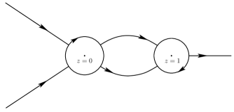
Figure 7. Jump contours for ${\bf R}(z)$ defined in (2.24) in the complex $z$-plane.

Riemann-Hilbert Problem 2.19.

Determine ${\bf R}(z)={\bf R}(z;s,\gamma)\in\mathbb{C}^{2\times 2}$ such that

1. $R(z)$ is analytic for $z\in\mathbb{C}\backslash\Sigma_{R}$ with square-integrable boundary values on the contour

   $$\Sigma_{R}:=\partial\mathbb{D}_{r}(0)\cup\partial\mathbb{D}_{r}(1)\cup(1+r,\infty)\cup\Big{(}\big{(}\Gamma_{2}\cup\Gamma_{4}\cup\gamma^{+}\cup\gamma^{-}\big{)}\cap\{z\in\mathbb{C}:|z|>r,|z-1|>r\}\Big{)},$$

   which is shown in Figure 7.

2. On the contour $\Sigma_{R}$, the boundary values ${\bf R}_{\pm}(z)$ are related via ${\bf R}_{+}(z)={\bf R}_{-}(z){\bf G}_{R}(z;s,\gamma)$ with

   $${\bf G}_{R}(z;s,\gamma) ={\bf P}^{(0)}(z)\big{(}{\bf P}^{(\infty)}(z)\big{)}^{-1},\hskip 96.84152ptz\in\partial\mathbb{D}_{r}(0);$$

   $${\bf G}_{R}(z;s,\gamma) ={\bf P}^{(1)}(z)\big{(}{\bf P}^{(\infty)}(z)\big{)}^{-1},\hskip 96.84152ptz\in\partial\mathbb{D}_{r}(1);$$

   $${\bf G}_{R}(z;s,\gamma) ={\bf P}^{(\infty)}(z)\begin{pmatrix}1&\mathrm{e}^{-t(\varkappa+2g(z))}\\ 0&1\end{pmatrix}\big{(}{\bf P}^{(\infty)}(z)\big{)}^{-1},\ \ \,z\in(1+r,\infty);$$

   $${\bf G}_{R}(z;s,\gamma) ={\bf P}^{(\infty)}(z)\begin{pmatrix}1&0\\ \mathrm{e}^{2tg(z)}&1\end{pmatrix}\big{(}{\bf P}^{(\infty)}(z)\big{)}^{-1},\hskip 32.52127ptz\in\big{(}\Gamma_{2}\cup\Gamma_{4}\big{)}\cap\{z\in\mathbb{C}:\,|z|>r\};$$

   $${\bf G}_{R}(z;s,\gamma) ={\bf P}^{(\infty)}(z)\begin{pmatrix}1&0\\ \mathrm{e}^{t(\phi(z)+\varkappa)}&1\end{pmatrix}\big{(}{\bf P}^{(\infty)}(z)\big{)}^{-1},\hskip 18.7898ptz\in\gamma^{\pm}\cap\{z\in\mathbb{C}:\,|z|>r,\ |z-1|>r\}.$$

   By construction, compare RHP 2.11, 2.12, and 2.14, there are no jumps inside $\mathbb{D}_{r}(0)\cup\mathbb{D}_{r}(1)$ and on $(-\infty,-r)\cup(r,1-r)$. Moreover, $R(z)$ is bounded at $z=0$.

3. As $z\rightarrow\infty$,

   $${\bf R}(z)=\begin{pmatrix}1&0\\ -2\mathrm{i}\nu|s|^{\frac{1}{2}}&1\end{pmatrix}(|s|z)^{-\frac{1}{4}\sigma_{3}}{\bf N}\left\{{\bf I}+{\bf X}_{1}(|s|z)^{-\frac{1}{2}}+\mathcal{O}\left(z^{-1}\right)\right\}\big{(}{\bf P}^{(\infty)}(z)\big{)}^{-1}={\bf I}+\mathcal{O}\left(z^{-\frac{1}{2}}\right).$$

Using standard small norm estimates, compare (2.10), (2.11), (2.12), and (2.16), we deduce

Proposition 2.20.

For any fixed $\gamma\in[0,1)$, there exist positive constants $t_{0}=t_{0}(\gamma)$ and $c=c(\gamma)$ such that

$$\|{\bf G}_{R}(\cdot;s,\gamma)-{\bf I}\|_{L^{2}\cap L^{\infty}(\Sigma_{R}\backslash\partial\mathbb{D}_{r}(0))}\leq\frac{c}{t^{\frac{2}{3}}}\text{ for all }t\geq t_{0}.$$

On the other hand, $\partial\mathbb{D}_{1}(0)$ has to be investigated more carefully. From (2.18),

$${\bf P}^{(0)}(z)\big{(}{\bf P}^{(\infty)}(z)\big{)}^{-1}={\bf I}+\mathcal{O}\left(t^{-\frac{2}{3}+2|\Re\nu|}\right),\ \ t\rightarrow\infty,$$

and

$$\nu=\frac{t\varkappa}{2\pi\mathrm{i}}=-\frac{1}{2\pi\mathrm{i}}\ln(1-\gamma)\in\mathrm{i}\mathbb{R},\ \ \gamma\in[0,1).$$

Hence, we can conclude

Proposition 2.21.

For any fixed $\gamma\in[0,1)$, there exist positive constants $t_{0}=t_{0}(\gamma)$ and $c=c(\gamma)$ such that

$$\|{\bf G}_{R}(\cdot;s,\gamma)-{\bf I}\|_{L^{2}\cap L^{\infty}(\partial\mathbb{D}_{r}(0))}\leq\frac{c}{t^{\frac{2}{3}}}\text{ for all }t\geq t_{0}.$$

The last Proposition, together with Proposition 2.20, ensures solvability of RHP 2.19 by general theory (see [28]).

Theorem 2.22.

For any fixed $\gamma\in[0,1)$, there exists $t_{0}=t_{0}(\gamma)>0$ and $c=c(\gamma)>0$ such that the ratio RHP 2.19 is uniquely solvable in $L^{2}(\Sigma_{R})$ for all $t\geq t_{0}$. We can compute its solution iteratively via the integral equation

$${\bf R}(z)={\bf I}+\frac{1}{2\pi\mathrm{i}}\int_{\Sigma_{R}}{\bf R}_{-}(\lambda)\big{(}{\bf G}_{R}(\lambda)-{\bf I}\big{)}\frac{{\mathrm{d}}\lambda}{\lambda-z},\ \ \ \lambda\in\mathbb{C}\backslash\Sigma_{R},$$

using that

$$\|{\bf R}_{-}(\cdot;s,\gamma)-{\bf I}\|_{L^{2}(\Sigma_{R})}\leq\frac{c}{t^{\frac{2}{3}}}\text{ for all }t\geq t_{0}.$$

This theorem will be central to the asymptotic evaluation of (1.15) as $s\rightarrow-\infty$. Before we carry out the underlying computations, we shall first derive two differential identities.

3. Differential identities

We connect the two logarithmic derivatives

$$\frac{\partial}{\partial s}\ln F_{2}(s,\gamma),\ \ \ \ \textnormal{respectively}\ \frac{\partial}{\partial\gamma}\ln F_{2}(s,\gamma),$$

with fixed $\gamma$, respectively $s$, to RHP 2.6. In this process it will be useful to recall the following well known facts about the “ring of integrable integral operators” (see [38]). The given kernel displays the structure (compare Remark 2.4)

$$\gamma K_{\textnormal{Ai}}(\lambda,\mu)=\frac{f^{T}(\lambda)h(\mu)}{\lambda-\mu};\ \ \ \ \ f(\lambda)=\binom{\Phi^{11}(\lambda)}{\Phi^{21}(\lambda)},\ \ h(\lambda)=\frac{\gamma}{2\pi\mathrm{i}}\binom{-\Phi^{21}(\lambda)}{\ \ \,\Phi^{11}(\lambda)},$$

and we observe that

$$\frac{\partial}{\partial s}\ln F_{2}(s,\gamma) = -\textnormal{trace}\,\left(\big{(}1-\gamma K_{\textnormal{Ai}}\upharpoonright_{L^{2}(s,\infty)}\big{)}^{-1}\gamma\frac{\partial}{\partial s}\big{(}K_{\textnormal{Ai}}\upharpoonright_{L^{2}(s,\infty)}\big{)}\right)$$

$$= \int_{s}^{\infty}\big{(}1-\gamma K_{\textnormal{Ai}}\big{)}^{-1}(s,\lambda)\gamma K_{\textnormal{Ai}}(\lambda,s)\,{\mathrm{d}}\lambda=R(s,s);$$

$$\frac{\partial}{\partial\gamma}\ln F_{2}(s,\gamma) = -\textnormal{trace}\,\left(\big{(}1-\gamma K_{\textnormal{Ai}}\upharpoonright_{L^{2}(s,\infty)}\big{)}^{-1}K_{\textnormal{Ai}}\upharpoonright_{L^{2}(s,\infty)}\right)=-\frac{1}{\gamma}\int_{s}^{\infty}R(\lambda,\lambda)\,{\mathrm{d}}\lambda.$$ (3.1)

Here, $1+R\upharpoonright_{L^{2}(s,\infty)}$ denotes the resolvent of the operator $\gamma K_{\textnormal{Ai}}\upharpoonright_{L^{2}(s,\infty)}$, i.e.

$$1+R\upharpoonright_{L^{2}(s,\infty)}=\big{(}1-\gamma K_{\textnormal{Ai}}\upharpoonright_{L^{2}(s,\infty)}\big{)}^{-1},$$

and we have the kernel representation

$$R(\lambda,\mu)=\frac{F^{T}(\lambda)H(\mu)}{\lambda-\mu},\ \ (\lambda,\mu)\in(s,\infty);\hskip 14.22636ptF=\big{(}1-\gamma K_{\textnormal{Ai}}\upharpoonright_{L^{2}(s,\infty)}\big{)}^{-1}f,\ \ H=\big{(}1-\gamma K_{\textnormal{Ai}}\upharpoonright_{L^{2}(s,\infty)}\big{)}^{-1}h.$$

Most importantly, the connection to RHP 2.1 is of the form

$${\bf Y}(z)={\bf I}-\int_{s}^{\infty}F(\lambda)h^{T}(\lambda)\frac{{\mathrm{d}}\lambda}{\lambda-z};\ \ \ \ F(z)={\bf Y}_{+}(z)f(z),\ \ H(z)=\big{(}{\bf Y}_{+}^{-1}\big{)}^{T}(z)h(z),\ \ z\in(s,\infty).$$

Proposition 3.1.

For fixed $\gamma\in\mathbb{R}$, we have

$$\frac{\partial}{\partial s}\ln F_{2}(s,\gamma)=\frac{\gamma}{2\pi\mathrm{i}}\big{(}{\bf X}^{-1}(z){\bf X}^{\prime}(z)\big{)}^{21}\Big{|}_{z\rightarrow s},\ \ \ \ (^{\prime})=\frac{{\mathrm{d}}}{{\mathrm{d}}z},$$

in terms of the solution ${\bf X}(z)$ to RHP 2.6, where the limit is taken with $\textnormal{arg}(z-s)\in(0,\frac{2\pi}{3})$.

Proof.

Note that

$$F(z)=\binom{X^{11}(z)}{X^{21}(z)},\ \ \ \ H(z)=\frac{\gamma}{2\pi\mathrm{i}}\binom{-X^{21}(z)}{\ \ \,X^{11}(z)},$$

where $X^{11}(z)$ and $X^{21}(z)$ are analytically continued from $\textnormal{arg}(z-s)\in(0,\frac{2\pi}{3})$ to the full complex plane. The stated identity follows now from

$$R(s,s)=\big{(}F^{T}\big{)}^{\prime}(z)H(z)\Big{|}_{z\rightarrow s},$$

in which the limit is taken in the same sector in the upper half-plane. ∎

For the second identity, we start from the central expression used in the derivation of Proposition 3.1,

$$R(\lambda,\lambda)=\frac{\gamma}{2\pi\mathrm{i}}\big{(}{\bf X}^{-1}(z){\bf X}^{\prime}(z)\big{)}^{21}\Big{|}_{z\rightarrow\lambda},\ \ \ \lambda\in(s,\infty);\hskip 21.33955pt(^{\prime})=\frac{{\mathrm{d}}}{{\mathrm{d}}z},$$ (3.2)

where again the limit is taken with $\textnormal{arg}(z-s)\in(0,\frac{2\pi}{3})$. Next, we replace the derivative terms by recalling the well-known differential equation associated with the function ${\bf X}(z)$ characterized through RHP 2.6,

$${\bf X}^{\prime}(z)=\Bigg{[}\begin{pmatrix}Y_{1}^{12}&1\vskip 3.0pt plus 1.0pt minus 1.0pt\\ z+Y_{1}^{22}-Y_{1}^{11}&-Y_{1}^{12}\end{pmatrix}+\frac{\gamma}{2\pi\mathrm{i}}\begin{pmatrix}-\widehat{X}^{11}(s)\widehat{X}^{21}(s)&\big{(}\widehat{X}^{11}(s)\big{)}^{2}\vskip 3.0pt plus 1.0pt minus 1.0pt\\ -\big{(}\widehat{X}^{21}(s)\big{)}^{2}&\widehat{X}^{11}(s)\widehat{X}^{21}(s)\end{pmatrix}\frac{1}{z-s}\Bigg{]}{\bf X}(z).$$

This equation follows directly from the observation that ${\bf X}^{\prime}{\bf X}^{-1}$ is single valued and analytic for $z\in\mathbb{C}\backslash\{s\}$, and hence can be computed from the asymptotics $z\rightarrow s,\infty$ by Liouville’s Theorem. Back in (3.2), we obtain

$$R(\lambda,\lambda) = \frac{\gamma}{2\pi\mathrm{i}}\Bigg{\{}-2X^{11}(\lambda)X^{21}(\lambda)\left[Y_{1}^{12}-\frac{\gamma}{2\pi\mathrm{i}}\frac{\widehat{X}^{11}(s)\widehat{X}^{21}(s)}{\lambda-s}\right]-\big{(}X^{21}(\lambda)\big{)}^{2}\left[1+\frac{\gamma}{2\pi\mathrm{i}}\frac{\big{(}\widehat{X}^{11}(s)\big{)}^{2}}{\lambda-s}\right]$$ (3.3)

$$\hskip 28.90755pt+\big{(}X^{11}(\lambda)\big{)}^{2}\left[\lambda+Y_{1}^{22}-Y_{1}^{11}-\frac{\gamma}{2\pi\mathrm{i}}\frac{\big{(}\widehat{X}^{21}(s)\big{)}^{2}}{\lambda-s}\right]\Bigg{\}},$$

and we now introduce the auxiliary function

$${\bf K}(z):=\frac{1}{2\pi\mathrm{i}}\int_{s}^{\infty}{\bf X}(\lambda)\bigl{(}\begin{smallmatrix}0&-1\\ 0&0\end{smallmatrix}\bigr{)}{\bf X}^{-1}(\lambda)\frac{{\mathrm{d}}\lambda}{\lambda-z},\ \ z\in\mathbb{C}\backslash[s,\infty).$$ (3.4)

In view of RHP 2.6, ${\bf K}(z)$ is well defined and we have the important identity

$${\bf K}(z)=\bigg{(}\frac{\partial}{\partial\gamma}{\bf X}(z)\bigg{)}{\bf X}^{-1}(z)=\bigg{(}\frac{\partial}{\partial\gamma}{\bf Y}(z)\bigg{)}{\bf Y}^{-1}(z),\ \ \ z\in\mathbb{C}\backslash[s,\infty).$$

Thus, on one hand, compare again RHP 2.6,

$${\bf K}(z)={\bf Y}_{1,\gamma}\,z^{-1}+\big{(}{\bf Y}_{2,\gamma}-{\bf Y}_{1,\gamma}{\bf Y}_{1}\big{)}z^{-2}+\mathcal{O}\left(z^{-3}\right),\ \ z\rightarrow\infty,\ z\notin[s,\infty);\ \ \ {\bf Y}_{\ell,\gamma}:=\frac{\partial}{\partial\gamma}{\bf Y}_{\ell},$$ (3.5)

and, on the other hand, from (3.4) in the same limit,

$${\bf K}(z)=\frac{1}{z}\frac{\mathrm{i}}{2\pi}\int_{s}^{\infty}{\bf X}(\lambda)\bigl{(}\begin{smallmatrix}0&-1\\ 0&0\end{smallmatrix}\bigr{)}{\bf X}^{-1}(\lambda)\,{\mathrm{d}}\lambda+\frac{1}{z^{2}}\frac{\mathrm{i}}{2\pi}\int_{s}^{\infty}\lambda\,{\bf X}(\lambda)\bigl{(}\begin{smallmatrix}0&-1\\ 0&0\end{smallmatrix}\bigr{)}{\bf X}^{-1}(\lambda)\,{\mathrm{d}}\lambda+\mathcal{O}\left(z^{-3}\right).$$ (3.6)

Hence, comparing entries in (3.5) and (3.6), one finds

$$Y_{1,\gamma}^{11}=\frac{\mathrm{i}}{2\pi}\int_{s}^{\infty}X^{11}(\lambda)X^{21}(\lambda)\,{\mathrm{d}}\lambda;\ \ \ \ \ \ \ \ Y_{1,\gamma}^{21}=\frac{\mathrm{i}}{2\pi}\int_{s}^{\infty}\big{(}X^{21}(\lambda)\big{)}^{2}\,{\mathrm{d}}\lambda;$$

$$-Y_{1,\gamma}^{12}=\frac{\mathrm{i}}{2\pi}\int_{s}^{\infty}\big{(}X^{11}(\lambda)\big{)}^{2}\,{\mathrm{d}}\lambda;\ \ \ \ \ \ \ \ \ \big{(}{\bf Y}_{1,\gamma}{\bf Y}_{1}\big{)}^{12}-Y_{2,\gamma}^{12}=\frac{\mathrm{i}}{2\pi}\int_{s}^{\infty}\lambda\,\big{(}X^{11}(\lambda)\big{)}^{2}\,{\mathrm{d}}\lambda.$$

These four identities are useful in the computation of (3.1) once we use (3.3). For the outstanding pieces we note that

$${\bf X}(\lambda)\bigl{(}\begin{smallmatrix}0&-1\\ 0&0\end{smallmatrix}\bigr{)}{\bf X}^{-1}(\lambda)=\widehat{{\bf X}}(s)\bigl{(}\begin{smallmatrix}0&-1\\ 0&0\end{smallmatrix}\bigr{)}\widehat{{\bf X}}^{-1}(s)+\mathcal{O}\left(\lambda-s\right)$$

as $\lambda\rightarrow s$ such that $\textnormal{arg}(\lambda-s)\in(0,\frac{2\pi}{3})\cup(\frac{4\pi}{3},2\pi)$. Hence, in the same limit,

$$2X^{11}(\lambda)X^{21}(\lambda)\widehat{X}^{11}(s)\widehat{X}^{21}(s)-\big{(}X^{21}(\lambda)\big{)}^{2}\big{(}\widehat{X}^{11}(s)\big{)}^{2}-\big{(}X^{11}(\lambda)\big{)}^{2}\big{(}\widehat{X}^{21}(s)\big{)}^{2}=\mathcal{O}\left(\lambda-s\right).$$

Define now the auxiliary function

$$\widehat{{\bf K}}(z) := {\bf K}(z)-\frac{1}{2\pi\mathrm{i}}\ln(z-s)\widehat{{\bf X}}(s)\bigl{(}\begin{smallmatrix}0&1\\ 0&0\end{smallmatrix}\bigr{)}\widehat{{\bf X}}^{-1}(s),\ \ \ \textnormal{arg}(z-s)\in(0,2\pi)$$

$$= \frac{1}{2\pi\mathrm{i}}\int_{s}^{\infty}\left[{\bf X}(\lambda)\bigl{(}\begin{smallmatrix}0&-1\\ 0&0\end{smallmatrix}\bigr{)}{\bf X}^{-1}(\lambda)-\widehat{{\bf X}}(s)\bigl{(}\begin{smallmatrix}0&-1\\ 0&0\end{smallmatrix}\bigr{)}\widehat{{\bf X}}^{-1}(s)\right]\frac{{\mathrm{d}}\lambda}{\lambda-z},\ \ z\in\mathbb{C}\backslash(s,\infty)$$

which is analytic at $z=s$, satisfying

$$\widehat{{\bf K}}(z)=\left(\frac{\partial}{\partial\gamma}\widehat{{\bf X}}(z)\right)\widehat{{\bf X}}^{-1}(z),\ \ z\rightarrow s.$$

Moreover, it provides us with the following identity:

$$\frac{1}{2\pi\mathrm{i}}\int_{s}^{\infty}\left[2X^{11}(\lambda)X^{21}(\lambda)\widehat{X}^{11}(s)\widehat{X}^{21}(s)-\big{(}X^{21}(\lambda)\big{)}^{2}\big{(}\widehat{X}^{11}(s)\big{)}^{2}-\big{(}X^{11}(\lambda)\big{)}^{2}\big{(}\widehat{X}^{21}(s)\big{)}^{2}\right]\frac{{\mathrm{d}}\lambda}{\lambda-s}$$

$$=\,\,2 \widehat{X}^{11}(s)\widehat{X}^{21}(s)\widehat{K}^{11}(s)-\big{(}\widehat{X}^{11}(s)\big{)}^{2}\widehat{K}^{21}(s)+\big{(}\widehat{X}^{21}(s)\big{)}^{2}\widehat{K}^{12}(s);\ \ \ \widehat{K}^{jk}(s):=\left(\left(\frac{\partial}{\partial\gamma}\widehat{{\bf X}}(s)\right)\widehat{{\bf X}}^{-1}(s)\right)^{jk}.$$

We summarize.

Proposition 3.2.

For fixed $s<0$, we have

$$\frac{\partial}{\partial\gamma}\ln F_{2}(s,\gamma) = -Y_{1,\gamma}^{11}Y_{1}^{12}+Y_{1,\gamma}^{12}Y_{1}^{11}-Y_{1,\gamma}^{21}-Y_{2,\gamma}^{12}$$

$$+\frac{\gamma}{2\pi\mathrm{i}}\left(\big{(}\widehat{X}^{11}(s)\big{)}^{2}\widehat{K}^{21}(s)-\big{(}\widehat{X}^{21}(s)\big{)}^{2}\widehat{K}^{12}(s)-2\widehat{X}^{11}(s)\widehat{X}^{21}(s)\widehat{K}^{11}(s)\right)$$

in terms of the asymptotic data ${\bf Y}_{1}$ and ${\bf Y}_{2}$ given in (2.1) as well as the singular data $\widehat{{\bf X}}(z)$ from (2.4).

4. Extraction of asymptotics via Proposition 3.1

In order to obtain structural information on the large negative $s$ behavior of $F_{2}(s,\gamma)$, we first use Proposition 3.1. Recall to this end the relevant transformations

$${\bf Y}(z)\mapsto{\bf X}(z)\mapsto{\bf T}(z)\mapsto{\bf S}(z)\mapsto{\bf L}(z)\mapsto{\bf R}(z),$$ (4.1)

and obtain in the first step with (2.5), (2.6), and (2.13),

$$\frac{\partial}{\partial s}\ln F_{2}(s,\gamma)=\frac{\gamma}{2\pi\mathrm{i}|s|}\mathrm{e}^{-2tg_{+}(0)}\Big{(}{\bf L}^{-1}(\lambda){\bf L}^{\prime}(\lambda)\Big{)}^{21}\bigg{|}_{\lambda\rightarrow 0},$$

where the limit is taken with $\textnormal{arg}\,\lambda\in(\frac{\pi}{3},\frac{2\pi}{3})$. After that, with (2.24),

$$\frac{\partial}{\partial s}\ln F_{2}(s,\gamma)= \frac{\gamma}{2\pi\mathrm{i}|s|}\mathrm{e}^{-2tg_{+}(0)}\Big{(}\big{(}{\bf P}^{(0)}(\lambda)\big{)}^{-1}\big{(}{\bf R}(0)\big{)}^{-1}{\bf R}^{\prime}(0){\bf P}^{(0)}(\lambda)\Big{)}^{21}\bigg{|}_{\lambda\rightarrow 0}$$

$$+\frac{\gamma}{2\pi\mathrm{i}|s|}\mathrm{e}^{-2tg_{+}(0)}\Big{(}\big{(}{\bf P}^{(0)}(\lambda)\big{)}^{-1}\big{(}{\bf P}^{(0)}(\lambda)\big{)}^{\prime}\Big{)}^{21}\bigg{|}_{\lambda\rightarrow 0}$$

using the same limit convention in both terms. The second term is computed explicitly using (2.20), (2.21), and (2.22),

$$\frac{\gamma}{2\pi\mathrm{i}|s|}\mathrm{e}^{-2tg_{+}(0)}\Big{(}\big{(}{\bf P}^{(0)}(\lambda)\big{)}^{-1}\big{(}{\bf P}^{(0)}(\lambda)\big{)}^{\prime}\Big{)}^{21}\bigg{|}_{\lambda\rightarrow 0}=\frac{v}{\pi}|s|^{\frac{1}{2}}+\frac{1}{|s|}\left[-\frac{3v^{2}}{8\pi^{2}}+\frac{v}{4\pi}\cos\big{(}2\phi(s,\gamma)\big{)}\right],$$ (4.2)

where we use the parameter $v=-\ln(1-\gamma)\in[0,+\infty)$ and the phase function

$$\phi(s,\gamma):=\frac{2}{3}|s|^{\frac{3}{2}}-\frac{v}{2\pi}\ln\big{(}8|s|^{\frac{3}{2}}\big{)}-\textnormal{arg}\,\Gamma\left(-\frac{iv}{2\pi}\right).$$ (4.3)

For the first term we need Theorem 2.22. More precisely, we write

$${\bf R}(z)=|s|^{-\frac{1}{4}\sigma_{3}}\widehat{{\bf R}}(z)|s|^{\frac{1}{4}\sigma_{3}},\ z\in\mathbb{C}\backslash\Sigma_{R};\ \ \ \ \ \ \|\widehat{{\bf R}}_{-}(\cdot;s,\gamma)-{\bf I}\|_{L^{2}(\Sigma_{R})}\leq\frac{c}{t}\text{ for all }t\geq t_{0},$$ (4.4)

and then deduce

$$\frac{\gamma}{2\pi\mathrm{i}|s|}\mathrm{e}^{-2tg_{+}(0)}\Big{(}\big{(}{\bf P}^{(0)}(\lambda)\big{)}^{-1}\big{(}{\bf R}(0)\big{)}^{-1}{\bf R}^{\prime}(0){\bf P}^{(0)}(\lambda)\Big{)}^{21}\bigg{|}_{\lambda\rightarrow 0}=\mathcal{O}\left(|s|^{-\frac{5}{2}}\right),\ \ s\rightarrow-\infty.$$ (4.5)

At this point we can combine (4.2) with (4.5) to find

$$\frac{\partial}{\partial s}\ln F_{2}(s,\gamma)=\frac{v}{\pi}|s|^{\frac{1}{2}}+\frac{1}{|s|}\left[-\frac{3v^{2}}{8\pi^{2}}+\frac{v}{4\pi}\cos\big{(}2\phi(s,\gamma)\big{)}\right]+\mathcal{O}\left(|s|^{-\frac{5}{2}}\right),\ \ s\rightarrow-\infty.$$ (4.6)

We integrate indefinitely with respect to $s$ to obtain the next result.

Proposition 4.1.

For any fixed $\gamma\in[0,1)$, there exist positive constants $t_{0}=t_{0}(\gamma)$ and $c=c(v)$ such that

$$\ln F_{2}(s,\gamma)=-\frac{2v}{3\pi}|s|^{\frac{3}{2}}+\frac{3v^{2}}{8\pi^{2}}\ln|s|+D(\gamma)+r(s,v)$$ (4.7)

for $t=|s|^{\frac{3}{2}}\geq t_{0}$ with $v=-\ln(1-\gamma)\in[0,+\infty)$. The term $D(\gamma)$ is independent of $s$, and the error term $r(s,v)$ satisfies

$$\big{|}r(s,v)\big{|}\leq\frac{c(v)}{|s|^{\frac{3}{2}}}\ \ \ \ \ \ \forall\,t\geq t_{0}.$$

Our next goal is the evaluation of the term $D(\gamma)$ in Proposition 4.1. This will be achieved in the following section.

5. Extraction of asymptotics via Proposition 3.2

We start from Proposition 3.2. For fixed $s<0$,

$$\frac{\partial}{\partial\gamma}\ln F_{2}(s,\gamma)=T_{1}(s,\gamma)+T_{2}(s,\gamma)+T_{3}(s,\gamma)$$

where we put for simplicity

$$T_{1}(s,\gamma):=-Y_{1,\gamma}^{11}Y_{1}^{12}+Y_{1,\gamma}^{12}Y_{1}^{11}-Y_{1,\gamma}^{21},\hskip 28.45274ptT_{2}(s,\gamma):=-Y_{2,\gamma}^{12},$$

and

$$T_{3}(s,\gamma):=\frac{\gamma}{2\pi\mathrm{i}}\left(\big{(}\widehat{X}^{11}(s)\big{)}^{2}\widehat{K}^{21}(s)-\big{(}\widehat{X}^{21}(s)\big{)}^{2}\widehat{K}^{12}(s)-2\widehat{X}^{11}(s)\widehat{X}^{21}(s)\widehat{K}^{11}(s)\right).$$ (5.1)

The idea is now to first evaluate all three $T_{j}(s,\gamma)$ asymptotically as $s\rightarrow-\infty$ with fixed $\gamma\in[0,1)$ and after that perform a definite integration with respect to $\gamma$,

$$\gamma\in[0,1):\ \ \ \ \ \ln F_{2}(s,\gamma)=\int_{0}^{\gamma}\frac{\partial}{\partial\gamma^{\prime}}\ln F_{2}(s,\gamma^{\prime}){\mathrm{d}}\gamma^{\prime}=\int_{0}^{\gamma}\big{(}T_{1}(s,\gamma^{\prime})+T_{2}(s,\gamma^{\prime})+T_{3}(s,\gamma^{\prime})\big{)}{\mathrm{d}}\gamma^{\prime}.$$ (5.2)

Comparing the so-obtained expansion for $\ln F_{2}(s,\gamma)$ to (4.7), we will obtain the unknown $D(\gamma)$.

5.1. Computation of $T_{1}(s,\gamma)$

We begin with the asymptotic evaluation of $T_{1}(s,\gamma)$ for which we trace back the transformations

$${\bf Y}(z)\mapsto{\bf X}(z)\mapsto{\bf T}(z)\mapsto{\bf S}(z)\mapsto{\bf L}(z).$$

This provides us with the following explicit identity for ${\bf Y}_{1}$ (compare (2.1)):

$${\bf Y}_{1}=|s|\begin{pmatrix}-2\nu^{2}&-2\mathrm{i}\nu|s|^{-\frac{1}{2}}\\ \frac{7}{48}|s|^{-1}+\frac{2}{3}\mathrm{i}\nu|s|^{\frac{1}{2}}(1-4\nu^{2})&2\nu^{2}\end{pmatrix}+|s|\begin{pmatrix}1&0\\ 2\mathrm{i}\nu|s|^{\frac{1}{2}}&1\end{pmatrix}{\bf J}_{1}\begin{pmatrix}1&0\\ -2\mathrm{i}\nu|s|^{\frac{1}{2}}&1\end{pmatrix},$$ (5.3)

where

$${\bf J}_{1}:=\frac{\mathrm{i}}{2\pi}\int_{\Sigma_{R}}{\bf R}_{-}(\lambda)\big{(}{\bf G}_{R}(\lambda)-{\bf I}\big{)}{\mathrm{d}}\lambda.$$

The last integral is then computed asymptotically with the help of Theorem 2.22, which amounts to a standard residue computation using (2.16) and (2.18). We summarize the results below.

Lemma 5.1.

As $s\rightarrow-\infty$,

$${\bf J}_{1}=|s|^{-\frac{1}{4}\sigma_{3}}\left\{\frac{1}{48t}\begin{pmatrix}-24\mathrm{i}\nu&-48\nu^{2}\\ -7&24\mathrm{i}\nu\end{pmatrix}+\frac{1}{2t}\begin{pmatrix}\mathrm{i}\nu\sin(2\phi)&-\nu^{2}-\mathrm{i}\nu\cos(2\phi)\\ \nu^{2}-\mathrm{i}\nu\cos(2\phi)&-\mathrm{i}\nu\sin(2\phi)\end{pmatrix}+\mathcal{O}\left(t^{-2}\right)\right\}|s|^{\frac{1}{4}\sigma_{3}}$$

with $\phi=\phi(s,\gamma)$ as in (4.3), $t=(-s)^{\frac{3}{2}}$. The error term is uniform with respect to $\gamma$ chosen from compact subsets of $[0,1)$, and it can be differentiated with respect to $\gamma$. In fact, after differentiation (with respect to $\gamma$), the error term is of order $\mathcal{O}\left(t^{-2}\ln t\right)$.

Substituting the result of this lemma into (5.3) gives:

Lemma 5.2.

As $s\rightarrow-\infty$, with the same statements about the error terms as in Lemma 5.1,

$$Y_{1}^{11}=-2\nu^{2}|s|-\frac{\mathrm{i}\nu}{2|s|^{\frac{1}{2}}}+\frac{3\mathrm{i}\nu^{3}}{|s|^{\frac{1}{2}}}+\frac{1}{2|s|^{\frac{1}{2}}}\big{(}\mathrm{i}\nu\sin(2\phi)-2\nu^{2}\cos(2\phi)\big{)}+\mathcal{O}\left(|s|^{-2}\right),$$

followed by

$$Y_{1}^{12}=-2\mathrm{i}\nu|s|^{\frac{1}{2}}-\frac{3\nu^{2}}{2|s|}-\frac{\mathrm{i}\nu}{2|s|}\cos(2\phi)+\mathcal{O}\big{(}|s|^{-\frac{5}{2}}\big{)},$$

and concluding with

$$Y_{1}^{21}=\frac{2}{3}\mathrm{i}\nu|s|^{\frac{3}{2}}(1-4\nu^{2})+\frac{5\nu^{2}}{2}-6\nu^{4}-2\nu^{2}\sin(2\phi)-\frac{\mathrm{i}\nu}{2}\cos(2\phi)-2\mathrm{i}\nu^{3}\cos(2\phi)+\mathcal{O}\big{(}|s|^{-\frac{3}{2}}\big{)}.$$

At this point, we only need to combine the results of Lemma 5.2 with the definition of $T_{1}(s,\gamma)$.

Proposition 5.3.

As $s\rightarrow-\infty$,

$$T_{1}(s,\gamma)= -\frac{2}{3}\mathrm{i}\nu_{\gamma}|s|^{\frac{3}{2}}+4\mathrm{i}\nu^{2}\nu_{\gamma}|s|^{\frac{3}{2}}+12\nu^{3}\nu_{\gamma}-5\nu\nu_{\gamma}+\cos(2\phi)\left\{2\nu^{2}\phi_{\gamma}+3\mathrm{i}\nu^{2}\nu_{\gamma}+\frac{1}{2}\mathrm{i}\nu_{\gamma}\right\}$$

$$+\sin(2\phi)\left\{-2\mathrm{i}\nu^{3}\phi_{\gamma}+4\nu\nu_{\gamma}-\mathrm{i}\nu\phi_{\gamma}\right\}+\mathcal{O}\left(|s|^{-\frac{3}{2}}\ln|s|\right),$$

and the error term is uniform with respect to $\gamma$ chosen from compact subsets of $[0,1)$.

5.2. Computation of $T_{2}(s,\gamma)$

Our strategy is the same as in the computation of $T_{1}(s,\gamma)$, however certain steps are more involved. First, after tracing back transformations, we obtain the exact identity

$${\bf Y}_{2}= \,|s|^{2}\begin{pmatrix}\frac{2}{3}\nu^{2}(\nu^{2}-1)-\frac{7\mathrm{i}\nu}{24}|s|^{-\frac{3}{2}}&\frac{4\mathrm{i}\nu}{3}(\nu^{2}-1)|s|^{-\frac{1}{2}}-\frac{5}{48}|s|^{-2}\\ \frac{4\mathrm{i}\nu}{15}(1-\nu^{2})(1-4\nu^{2})|s|^{\frac{1}{2}}+\frac{7}{48}(1+2\nu^{2})|s|^{-1}&-\frac{2}{3}\nu^{2}(\nu^{2}-1)\end{pmatrix}-|s|{\bf Y}_{1}$$

$$+|s|^{2}\begin{pmatrix}1&0\\ 2\mathrm{i}\nu|s|^{\frac{1}{2}}\end{pmatrix}{\bf J}_{1}\begin{pmatrix}1&0\\ -2\mathrm{i}\nu|s|^{\frac{1}{2}}&1\end{pmatrix}\begin{pmatrix}-2\nu^{2}&-2\mathrm{i}\nu|s|^{-\frac{1}{2}}\\ \frac{7}{48}|s|^{-1}+\frac{2}{3}\mathrm{i}\nu|s|^{\frac{1}{2}}(1-4\nu^{2})&2\nu^{2}\end{pmatrix}$$

$$+|s|^{2}\begin{pmatrix}1&0\\ 2\mathrm{i}\nu|s|^{\frac{1}{2}}&1\end{pmatrix}{\bf J}_{2}\begin{pmatrix}1&0\\ -2\mathrm{i}\nu|s|^{\frac{1}{2}}&1\end{pmatrix},$$ (5.4)

where

$${\bf J}_{2}:=\frac{\mathrm{i}}{2\pi}\int_{\Sigma_{R}}{\bf R}_{-}(\lambda)\big{(}{\bf G}_{R}(\lambda)-{\bf I}\big{)}\lambda\,{\mathrm{d}}\lambda,$$

and ${\bf Y}_{1}$ and ${\bf J}_{1}$ have appeared previously in (5.3). After that, we have the following analogue of Lemma 5.1.

Lemma 5.4.

As $s\rightarrow-\infty$,

$${\bf J}_{2}=|s|^{-\frac{1}{4}\sigma_{3}}\left\{\frac{1}{48t}\begin{pmatrix}-24\mathrm{i}\nu&5-48\nu^{2}\\ -7&24\mathrm{i}\nu\end{pmatrix}+\mathcal{O}\left(t^{-2}\right)\right\}|s|^{\frac{1}{4}\sigma_{3}},$$

and the error term is uniform with respect to $\gamma$ chosen from compact subsets of $[0,1)$.

Now we substitute all obtained formulæ  into (5.4), which leads to

Lemma 5.5.

As $s\rightarrow-\infty$,

$$Y_{2}^{12}=\frac{4}{3}\mathrm{i}\nu^{3}|s|^{\frac{3}{2}}+\frac{2}{3}\mathrm{i}\nu|s|^{\frac{3}{2}}-\frac{1}{2}\nu^{2}+3\nu^{4}+\cos(2\phi)\left\{\frac{1}{2}\mathrm{i}\nu+\mathrm{i}\nu^{3}\right\}+\nu^{2}\sin(2\phi)+\mathcal{O}\left(|s|^{-\frac{3}{2}}\right),$$

where the error term is uniform with respect to $\gamma$ chosen from compact subsets of $[0,1)$ and can be differentiated with respect to $\gamma$.

At this point, we are left to summarize our current results.

Proposition 5.6.

As $s\rightarrow-\infty$,

$$T_{2}(s,\gamma)= -\frac{2}{3}\mathrm{i}\nu_{\gamma}|s|^{\frac{3}{2}}-4\mathrm{i}\nu^{2}\nu_{\gamma}|s|^{\frac{3}{2}}-12\nu^{3}\nu_{\gamma}+\nu\nu_{\gamma}+\cos(2\phi)\left\{-2\nu^{2}\phi_{\gamma}-3\mathrm{i}\nu^{2}\nu_{\gamma}-\frac{1}{2}\mathrm{i}\nu_{\gamma}\right\}$$

$$+\sin(2\phi)\left\{2\mathrm{i}\nu^{3}\phi_{\gamma}-2\nu\nu_{\gamma}+\mathrm{i}\nu\phi_{\gamma}\right\}+\mathcal{O}\left(|s|^{-\frac{3}{2}}\ln|s|\right),$$

and the error term is uniform with respect to $\gamma$ chosen from compact subsets of $[0,1)$.

5.3. Computation of $T_{3}(s,\gamma)$

For the last part we require the following exact identity, compare (2.4), (2.5), (2.6), (2.13), (2.20), (2.21), (2.24):

$$\widehat{{\bf X}}(s)=\begin{pmatrix}1&0\\ 2\mathrm{i}\nu|s|^{\frac{1}{2}}&1\end{pmatrix}{\bf R}(0){\bf E}^{(0)}(0)\widehat{\Psi}(0)\begin{pmatrix}1&\frac{\gamma}{2\pi\mathrm{i}}\ln(2|s|^{\frac{1}{2}})\\ 0&1\end{pmatrix}.$$ (5.5)

This formula implies at once that $\det\widehat{{\bf X}}(s)=1$, which in turn leads to a simplified identity for $T_{3}(s,\gamma)$.

Lemma 5.7.

We have for $T_{3}(s,\gamma)$ as defined in (5.1), see also Proposition 3.2,

$$T_{3}(s,\gamma)=\frac{\gamma}{2\pi\mathrm{i}}\Big{(}\widehat{X}^{11}(s)\widehat{X}^{21}_{\gamma}(s)-\widehat{X}^{11}_{\gamma}(s)\widehat{X}^{21}(s)\Big{)}.$$

Proof.

Note that

$$\widehat{K}^{11}(s)=\widehat{X}_{\gamma}^{11}(s)\widehat{X}^{22}(s)-\widehat{X}_{\gamma}^{12}(s)\widehat{X}^{21}(s),\ \ \ \ \ \ \widehat{K}^{12}(s)=-\widehat{X}^{11}_{\gamma}(s)\widehat{X}^{12}(s)+\widehat{X}^{12}_{\gamma}(s)\widehat{X}^{11}(s),$$

and

$$\widehat{K}^{21}(s)=\widehat{X}^{21}_{\gamma}(s)\widehat{X}^{22}(s)-\widehat{X}^{22}_{\gamma}(s)\widehat{X}^{21}(s).$$

If we now use $\widehat{X}^{11}(s)\widehat{X}^{22}(s)-\widehat{X}^{12}(s)\widehat{X}^{21}(s)\equiv 1$, which leads to

$$\widehat{X}_{\gamma}^{11}(s)\widehat{X}^{22}(s)-\widehat{X}_{\gamma}^{12}(s)\widehat{X}^{21}(s)=-\big{(}\widehat{X}^{11}(s)\widehat{X}_{\gamma}^{22}(s)-\widehat{X}^{12}(s)\widehat{X}_{\gamma}^{21}(s)\big{)},$$

then the identity follows directly from (5.1) after simplification. ∎

We now evaluate the outstanding matrix elements $\widehat{X}^{11}(s)$ and $\widehat{X}^{21}(s)$ through (5.5) by referring once more to Theorem 2.22:

Lemma 5.8.

For any fixed $\gamma\in[0,1)$, as $s\rightarrow-\infty$,

$${\bf R}(0)=|s|^{-\frac{1}{4}\sigma_{3}}\left\{{\bf I}+\mathcal{O}\left(t^{-1}\right)\right\}|s|^{\frac{1}{4}\sigma_{3}}.$$

Thus, after simplification, using in particular the phase function $\phi=\phi(s,\gamma)$ in (4.3),

Lemma 5.9.

As $s\rightarrow-\infty$,

$$\widehat{X}^{11}(s)=|s|^{-\frac{1}{4}}\left\{\sqrt{\frac{\mathrm{i}\pi\nu}{\gamma}}\,\big{(}\mathrm{e}^{\mathrm{i}\phi}-\mathrm{i}\mathrm{e}^{-\mathrm{i}\phi}\big{)}+\mathcal{O}\left(t^{-1}\right)\right\}$$

and

$$\widehat{X}^{21}(s)=|s|^{\frac{1}{4}}\left\{\sqrt{\frac{\mathrm{i}\pi\nu}{\gamma}}\,\big{(}\mathrm{i}(2\nu-1)\mathrm{e}^{\mathrm{i}\phi}+(2\nu+1)\mathrm{e}^{-\mathrm{i}\phi}\big{)}+\mathcal{O}\left(t^{-1}\right)\right\},$$

where all error terms are uniform with respect to $\gamma$ chosen from compact subsets of $[0,1)$. Again, they are also differentiable with respect to $\gamma$, subject to error correction.

The final step of our computation consists in combining Lemma 5.9 with Lemma 5.7. The result is as follows.

Proposition 5.10.

As $s\rightarrow-\infty$,

$$T_{3}(s,\gamma)=-2\nu\nu_{\gamma}\sin(2\phi)+2\nu\nu_{\gamma}-2\mathrm{i}\nu\phi_{\gamma}+\mathcal{O}\left(|s|^{-\frac{3}{2}}\ln|s|\right)$$

with an error term that is uniform with respect to $\gamma$ chosen from compact subsets of $[0,1)$.

5.4. Evaluation of $D(\gamma)$

The final expression for $D(\gamma)$ is obtained by combining Propositions 5.3, 5.6, and 5.10. We have

$$\begin{split}\frac{\partial}{\partial\gamma}\ln F_{2}(s,\gamma)=&T_{1}(s,\gamma)+T_{2}(s,\gamma)+T_{3}(s,\gamma)\\ =&-\frac{4\mathrm{i}}{3}\nu_{\gamma}|s|^{\frac{3}{2}}-2\nu\nu_{\gamma}-2\mathrm{i}\nu\phi_{\gamma}+\mathcal{O}\left(|s|^{-\frac{3}{2}}\ln|s|\right)\\ =&-\frac{2v_{\gamma}}{3\pi}|s|^{\frac{3}{2}}+\frac{vv_{\gamma}}{2\pi^{2}}\ln\big{(}8|s|^{\frac{3}{2}}\big{)}+\frac{vv_{\gamma}}{2\pi^{2}}+\frac{v}{\pi}\frac{{\mathrm{d}}}{{\mathrm{d}}\gamma}\textnormal{arg}\,\Gamma\left(-\frac{\mathrm{i}v}{2\pi}\right)+\mathcal{O}\left(|s|^{-\frac{3}{2}}\ln|s|\right),\end{split}$$ (5.6)

where we used the definitions of $\phi=\phi(s,\gamma)$ from (4.3) and $v=-\ln(1-\gamma)=2\pi\mathrm{i}\nu$ in the last equality. Since $v|_{\gamma=0}=0$, we now integrate and derive, compare (5.2),

$$\ln F_{2}(s,\gamma)=-\frac{2v}{3\pi}|s|^{\frac{3}{2}}+\frac{v^{2}}{4\pi^{2}}\ln\big{(}8|s|^{\frac{3}{2}}\big{)}+\frac{v^{2}}{4\pi^{2}}-\frac{1}{\pi}\int_{0}^{\gamma}v(\gamma^{\prime})\left\{\frac{{\mathrm{d}}}{{\mathrm{d}}\gamma^{\prime}}\,\textnormal{arg}\,\Gamma\left(\frac{\mathrm{i}v(\gamma^{\prime})}{2\pi}\right)\right\}{\mathrm{d}}\gamma^{\prime}+\mathcal{O}\left(|s|^{-\frac{3}{2}}\ln|s|\right).$$

This last identity can then be further simplified by referring to the Barnes $G$-function [43]. This special function satisfies the following useful identity

$$z\in\mathbb{C}:\ \Re z>-1,\ \ \ \ \ \int_{0}^{z}\ln\Gamma(1+x)\,{\mathrm{d}}x=\frac{z}{2}\ln(2\pi)-\frac{z}{2}(z+1)+z\ln\Gamma(1+z)-\ln G(1+z),$$ (5.7)

and allows us to obtain the next proposition.

Proposition 5.11.

For any fixed $\gamma\in[0,1)$, with $v=v(\gamma)=-\ln(1-\gamma)$,

$$\frac{v^{2}}{4\pi^{2}}-\frac{1}{\pi}\int_{0}^{\gamma}v(\gamma^{\prime})\left\{\frac{{\mathrm{d}}}{{\mathrm{d}}\gamma^{\prime}}\,\textnormal{arg}\,\Gamma\left(\frac{\mathrm{i}v(\gamma^{\prime})}{2\pi}\right)\right\}{\mathrm{d}}\gamma^{\prime}=\ln\big{(}G\Big{(}1+\frac{\mathrm{i}v}{2\pi}\Big{)}G\Big{(}1-\frac{\mathrm{i}v}{2\pi}\Big{)}\big{)}.$$

Proof.

Using that

$$\Gamma\left(\frac{\mathrm{i}v}{2\pi}\right)\left\{\Gamma\left(-\frac{\mathrm{i}v}{2\pi}\right)\right\}^{-1}=\exp\left[2\mathrm{i}\,\textnormal{arg}\,\Gamma\left(\frac{\mathrm{i}v}{2\pi}\right)\right],$$

we need to evaluate

$$\int_{0}^{\gamma}v(\gamma^{\prime})\left\{\frac{{\mathrm{d}}}{{\mathrm{d}}\gamma^{\prime}}\,\textnormal{arg}\,\Gamma\left(\frac{\mathrm{i}}{2\pi}v(\gamma^{\prime})\right)\right\}{\mathrm{d}}\gamma^{\prime}=\frac{1}{2\mathrm{i}}\int_{0}^{\gamma}v(\gamma^{\prime})\left\{\frac{{\mathrm{d}}}{{\mathrm{d}}\gamma^{\prime}}\ln\frac{\Gamma(1+\frac{\mathrm{i}}{2\pi}v(\gamma^{\prime}))}{\Gamma(1-\frac{\mathrm{i}}{2\pi}v(\gamma^{\prime}))}\right\}{\mathrm{d}}\gamma^{\prime}.$$

The last integral is exactly of the form (5.7) after integration by parts, so the stated identity follows at once. ∎

The last proposition concludes our asymptotic evaluation of $F_{2}(s,\gamma)$. We have

$$\ln F_{2}(s,\gamma)=-\frac{2v}{3\pi}|s|^{\frac{3}{2}}+\frac{v^{2}}{4\pi^{2}}\ln\big{(}8|s|^{\frac{3}{2}}\big{)}+\ln\left(G\Big{(}1+\frac{\mathrm{i}v}{2\pi}\Big{)}G\Big{(}1-\frac{\mathrm{i}v}{2\pi}\Big{)}\right)+\mathcal{O}\left(|s|^{-\frac{3}{2}}\ln|s|\right).$$ (5.8)

Comparing with (4.7) gives the following.

Corollary 5.12.

For any fixed $\gamma\in[0,1)$,

$$D(\gamma)=\frac{3v^{2}}{4\pi^{2}}\ln 2+\ln\left(G\Big{(}1+\frac{\mathrm{i}v}{2\pi}\Big{)}G\Big{(}1-\frac{\mathrm{i}v}{2\pi}\Big{)}\right),\ \ \ v=-\ln(1-\gamma)\in[0,+\infty).$$

In the end, combining (5.8) with Proposition 4.1 gives the desired result.

Theorem 5.13.

For any fixed $\gamma\in[0,1)$, there exist positive constants $t_{0}=t_{0}(\gamma)$ and $c=c(v)$ such that

$$\ln F_{2}(s,\gamma)=-\frac{2v}{3\pi}|s|^{\frac{3}{2}}+\frac{v^{2}}{4\pi^{2}}\ln\big{(}8|s|^{\frac{3}{2}}\big{)}+\ln\left(G\Big{(}1+\frac{\mathrm{i}v}{2\pi}\Big{)}G\Big{(}1-\frac{\mathrm{i}v}{2\pi}\Big{)}\right)+r(s,v)$$ (5.9)

for $t=|s|^{\frac{3}{2}}\geq t_{0}$ with $v=-\ln(1-\gamma)\in[0,+\infty)$ and in terms of the Barnes $G$-function. The error term is differentiable with respect to $s$ and satisfies

$$\big{|}r(s,v)\big{|}\leq\frac{c(v)}{|s|^{\frac{3}{2}}}\ \ \ \ \ \ \forall\,t\geq t_{0}.$$

The last theorem was derived under the assumption that $\gamma\in[0,1)$ is kept fixed throughout. However, as we shall prove in the next section, the leading order behavior (5.9) is still valid as $\gamma\uparrow 1$ at a certain (not too fast) rate.

6. Extension of Theorem 5.13

In order to allow for certain values of $v=-\ln(1-\gamma)\rightarrow+\infty$ we repeat all steps leading to the ratio problem RHP 2.19. However, now special care has to be given to the underlying error estimates.

6.1. Preliminary estimates

Consider ${\bf G}_{R}(z;s,\gamma)$ for $z\in\partial\mathbb{D}_{r}(1)$, as $s\rightarrow-\infty$, from (2.17), see also (2.16),

$${\bf G}_{R}(z;s,\gamma)-{\bf I}={\bf P}^{(\infty)}(z)\mathrm{e}^{-\frac{t}{2}\varkappa\sigma_{3}}\left\{\frac{1}{48\zeta^{\frac{3}{2}}(z)}\begin{pmatrix}1&6\mathrm{i}\\ 6\mathrm{i}&-1\end{pmatrix}+{\bf\mathcal{E}}^{(1)}(z;s)\right\}\mathrm{e}^{\frac{t}{2}\varkappa\sigma_{3}}\big{(}{\bf P}^{(\infty)}(z)\big{)}^{-1},$$ (6.1)

where the error term $\mathcal{E}^{(1)}(z;s)$ is $v$-independent. To estimate the behavior with respect to $v$, we thus only need to recall (2.14):

$$z\in\partial\mathbb{D}_{r}(1),\ \ 0<r<\frac{1}{4}:\ \ \ \ \big{|}\mathcal{D}(z)\mathrm{e}^{\frac{t}{2}\varkappa}\big{|}=\exp\left[\frac{v}{2\pi}\arctan\left(\frac{2\sqrt{r}\cos(\frac{1}{2}\textnormal{arg}(z-1))}{1-r}\right)\right].$$

This shows that a contracting radius $r=r_{t}=t^{-\frac{2}{3}+\epsilon}$ with $0<\epsilon<\frac{2}{3}$ in the scaling region

$$t\geq t_{0},\ \ 0\leq v<t^{\frac{1}{3}-\frac{\epsilon}{2}}$$ (6.2)

ensures on one end that

$$z\in\partial\mathbb{D}_{r_{t}}(1):\ \ \ \ \big{|}\mathcal{D}(z)\mathrm{e}^{\frac{t}{2}\varkappa}\big{|}^{\pm 1}=\exp\left[\pm\frac{v\sqrt{r}}{\pi}\cos\left(\frac{1}{2}\textnormal{arg}(z-1)\right)\right]\big{(}1+\mathcal{O}\big{(}vr^{\frac{3}{2}}\big{)}\big{)}=\mathcal{O}(1).$$

On the other end, we (still) have for $z\in\partial\mathbb{D}_{r_{t}}(1)$ that

$$|\zeta(z)|\geq c_{3}t^{\frac{2}{3}}r_{t}=c_{3}t^{\epsilon}\rightarrow+\infty\ \ \ \textnormal{as}\ \ t\rightarrow+\infty.$$

Combining these bounds in (6.1) gives the following.

Proposition 6.1.

For every fixed $0<\epsilon<\frac{2}{3}$, there exist $t_{0}>0$ and $c>0$ such that

$$\|{\bf G}_{R}(\cdot;s,\gamma)-{\bf I}\|_{L^{2}\cap L^{\infty}(\partial\mathbb{D}_{r_{t}}(1))}\leq\frac{c}{t^{\epsilon}}\text{ for all }t\geq t_{0},\ \ 0\leq v<t^{\frac{1}{3}-\frac{\epsilon}{2}}.$$

The corresponding argument for $z\in\partial\mathbb{D}_{r}(0)$ is similar but more involved since $\Psi(\zeta)$ in (2.19) already depends on $\gamma$ while $\Phi(\zeta)$, see (2.3), did not. This difference requires us to work with the full asymptotic series in condition (4) of RHP 2.15. From [43], as $\zeta\rightarrow\infty$,

$$\Psi(\zeta)\sim \left[{\bf I}+\mathrm{e}^{\mathrm{i}\frac{\pi}{2}\nu\sigma_{3}}\sum_{k=1}^{\infty}\begin{pmatrix}((\nu)_{k})^{2}\mathrm{e}^{\mathrm{i}\frac{\pi}{2}k}&((1-\nu)_{k-1})^{2}k\,\mathrm{e}^{-\mathrm{i}\frac{\pi}{2}k}\frac{\Gamma(1-\nu)}{\Gamma(\nu)}\\ ((1+\nu)_{k-1})^{2}k\,\mathrm{e}^{\mathrm{i}\frac{\pi}{2}k}\frac{\Gamma(1+\nu)}{\Gamma(-\nu)}&((-\nu)_{k})^{2}\mathrm{e}^{-\mathrm{i}\frac{\pi}{2}k}\end{pmatrix}\frac{\zeta^{-k}}{k!}\mathrm{e}^{-\mathrm{i}\frac{\pi}{2}\nu\sigma_{3}}\right]$$

$$\times\,\zeta^{-\nu\sigma_{3}}\mathrm{e}^{-\frac{\mathrm{i}}{2}\zeta\sigma_{3}}\begin{cases}\Bigl{(}\begin{smallmatrix}\mathrm{e}^{\mathrm{i}\frac{3\pi}{2}\nu}&0\\ 0&\mathrm{e}^{-\mathrm{i}\frac{\pi}{2}\nu}\end{smallmatrix}\Bigr{)},&\textnormal{arg}\,\zeta\in(0,\pi)\vskip 3.0pt plus 1.0pt minus 1.0pt\\ \Bigl{(}\begin{smallmatrix}0&-\mathrm{e}^{\mathrm{i}\frac{\pi}{2}\nu}\\ \mathrm{e}^{\mathrm{i}\frac{\pi}{2}\nu}&0\end{smallmatrix}\Bigr{)},&\textnormal{arg}\,\zeta\in(-\pi,0),\end{cases}$$

where $(\nu)_{k}:=\nu(\nu+1)(\nu+2)\cdot\ldots\cdot(\nu+k-1)$ is the Pochhammer symbol and $\nu=2\pi\mathrm{i}v\in\mathrm{i}\mathbb{R}$. Now we use (2.21) and (2.23) so that first for $z\in\partial\mathbb{D}_{r}(0):\textnormal{arg}\,z\in(0,\pi)$, as $s\rightarrow-\infty$,

$${\bf N}^{-1} (|s|(z-1))^{\frac{1}{4}\sigma_{3}}\Big{(}{\bf G}_{R}(z;s,\gamma)-{\bf I}\Big{)}(|s|(z-1))^{-\frac{1}{4}\sigma_{3}}{\bf N}$$

$$\sim\,\sum_{k=1}^{\infty}\begin{pmatrix}((\nu)_{k})^{2}\mathrm{e}^{\mathrm{i}\frac{\pi}{2}k}&-\nu((1-\nu)_{k-1})^{2}k\,\mathrm{e}^{-\mathrm{i}\frac{\pi}{2}k}(f^{+}(z;s,\gamma))^{-1}\vskip 3.0pt plus 1.0pt minus 1.0pt\\ \nu((1+\nu)_{k-1})^{2}k\,\mathrm{e}^{\mathrm{i}\frac{\pi}{2}k}f^{+}(z;s,\gamma)&((-\nu)_{k})^{2}\mathrm{e}^{-\mathrm{i}\frac{\pi}{2}k}\end{pmatrix}\frac{\zeta^{-k}}{k!}$$ (6.3)

with

$$f^{+}(z;s,\gamma):=\mathrm{e}^{-\mathrm{i}\frac{4}{3}t-2\mathrm{i}\textnormal{arg}\,\Gamma(-\nu)}\mathrm{e}^{2\pi\mathrm{i}\nu}\big{(}\zeta(z)\big{)}^{-2\nu}\big{(}\mathcal{D}(z)\big{)}^{2},\ \ z\in\partial\mathbb{D}_{r}(0):\ \textnormal{arg}\,z\in(0,\pi).$$

Note that for $z\in\partial\mathbb{D}_{r}(0)$,

$$\big{|}f^{+}(z;s,\gamma)\big{|}= \,\mathrm{e}^{v}\exp\left[-\frac{v}{\pi}\textnormal{arg}\,\zeta(z)+\frac{v}{\pi}\textnormal{arg}\,\left(\frac{(z-1)^{\frac{1}{2}}-\mathrm{i}}{(z-1)^{\frac{1}{2}}+\mathrm{i}}\right)\right]$$

$$= \,\mathrm{e}^{v}\exp\left[-\frac{v}{\pi}\textnormal{arg}\,\zeta(z)-\frac{v}{\pi}\arccos\left(\frac{1}{r}\big{\{}|z-1|-1\big{\}}\right)\right],$$ (6.4)

and likewise

$$|z-1|=\sqrt{1-2r\cos(\textnormal{arg}\,z)+r^{2}}.$$

Thus, as $r\downarrow 0$ with $\textnormal{arg}\,z\in(0,\pi)$,

$$\arccos\left(\frac{1}{r}\big{(}|z-1|-1\big{)}\right)=\pi-\textnormal{arg}\,z-\frac{r}{2}\sin(\textnormal{arg}\,z)+\mathcal{O}\left(r^{2}\right),$$

leading to (compare also (2.22))

$$\big{|}f^{+}(z;s,\gamma)\big{|}= \,\exp\left[-\frac{v}{\pi}\textnormal{arg}\left(\frac{\zeta(z)}{z}\right)+\frac{vr}{2\pi}\sin(\textnormal{arg}\,z)\right]\big{(}1+\mathcal{O}\left(vr^{2}\right)\big{)}$$

$$= \,\exp\left[\frac{3vr}{4\pi}\sin(\textnormal{arg}\,z)\right]\big{(}1+\mathcal{O}\left(vr^{2}\right)\big{)},$$ (6.5)

provided that $vr\downarrow 0$. The situation is similar in the lower half plane; instead of (6.3) we have now for $z\in\partial\mathbb{D}_{r}(0):\ \textnormal{arg}\,z\in(-\pi,0)$, as $s\rightarrow-\infty$,

$${\bf N}^{-1} (|s|(z-1))^{\frac{1}{4}\sigma_{3}}\Big{(}{\bf G}_{R}(z;s,\gamma)-{\bf I}\Big{)}(|s|(z-1))^{-\frac{1}{4}\sigma_{3}}{\bf N}$$

$$\sim\,\sum_{k=1}^{\infty}\begin{pmatrix}((-\nu)_{k})^{2}\mathrm{e}^{-\mathrm{i}\frac{\pi}{2}k}&-\nu((1+\nu)_{k-1})^{2}k\,\mathrm{e}^{\mathrm{i}\frac{\pi}{2}k}(f^{-}(z;s,\gamma))^{-1}\vskip 3.0pt plus 1.0pt minus 1.0pt\\ \nu((1-\nu)_{k-1})^{2}k\,\mathrm{e}^{-\mathrm{i}\frac{\pi}{2}k}f^{-}(z;s,\gamma)&((\nu)_{k})^{2}\mathrm{e}^{\mathrm{i}\frac{\pi}{2}k}\end{pmatrix}\frac{\zeta^{-k}}{k!}$$ (6.6)

with

$$f^{-}(z;s,\gamma):=\mathrm{e}^{\mathrm{i}\frac{4}{3}t+2\mathrm{i}\textnormal{arg}\,\Gamma(-\nu)}\mathrm{e}^{2\pi\mathrm{i}\nu}\big{(}\zeta(z)\big{)}^{2\nu}\big{(}\mathcal{D}(z)\big{)}^{2},\ \ z\in\partial\mathbb{D}_{r}(0):\ \textnormal{arg}\,z\in(-\pi,0).$$

Applying the same geometrical reasoning as above, we deduce this time

$$\big{|}f^{-}(z;s,\gamma)\big{|}=\exp\left[-\frac{3vr}{4\pi}\sin(\textnormal{arg}\,z)\right]\big{(}1+\mathcal{O}\left(vr^{2}\right)\big{)},\ \ vr\downarrow 0.$$

Thus, here we choose a contracting radius $r=\hat{r}_{t}=t^{-\frac{1}{3}}$ so that, subject to (6.2),

$$0\leq|vr|<t^{-\frac{\epsilon}{2}}\downarrow 0;\ \ \ \ \ \ \ \ \ \ \ z\in\partial\mathbb{D}_{\hat{r}_{t}}(0):\ \ |\zeta(z)|\geq ctr=ct^{\frac{2}{3}}\rightarrow+\infty.$$ (6.7)

Hence, with (6.3) and (6.6),

$$\Big{\|}|s|^{\frac{1}{4}\sigma_{3}}\big{(}{\bf G}_{R}(z;s,\gamma)-{\bf I}\big{)}|s|^{-\frac{1}{4}\sigma_{3}}\Big{\|}\leq c\left\{\frac{v}{rt}\left\|\begin{pmatrix}v&|f^{\pm}(z;s,\gamma)|^{-1}\\ |f^{\pm}(s;z,\gamma)|&v\end{pmatrix}\right\|+\mathcal{E}^{(0)}(z;s,\gamma)\right\},\ \ z\in\partial\mathbb{D}_{\hat{r}_{t}}(0).$$

Estimates for the error term $\mathcal{E}^{(0)}(z;s,\gamma)$ follow from known error estimates for the confluent hypergeometric function, see e.g. [43]: there exist $t_{0}>0$ and constants $c_{j}>0$ such that

$$\big{\|}\mathcal{E}^{(0)}(z;s,\gamma)\big{\|}\leq c_{1}\mathrm{e}^{c_{2}v-c_{3}rt}\leq c_{1}\mathrm{e}^{-c_{4}t^{\frac{2}{3}}}\text{ for all }t\geq t_{0},\ \ 0\leq v<t^{\frac{1}{3}-\frac{\epsilon}{2}}\ \ \textnormal{with}\ \ \epsilon\in\left(0,\frac{2}{3}\right)\ \textnormal{fixed}.$$

But in the same scaling regime, compare (6.7), $|f^{\pm}(z;s,\gamma)|^{\pm 1}\rightarrow 1$. Together these show the following.

Proposition 6.2.

For every fixed $0<\epsilon<\frac{2}{3}$, there exist $t_{0}>0$ and $c>0$ such that

$$\Big{\|}|s|^{\frac{1}{4}\sigma_{3}}\big{(}{\bf G}_{R}(\cdot;s,\gamma)-{\bf I}\big{)}|s|^{-\frac{1}{4}\sigma_{3}}\Big{\|}_{L^{2}\cap L^{\infty}(\partial\mathbb{D}_{\hat{r}_{t}}(0))}\leq c\,v^{2}\,t^{-\frac{2}{3}}\text{ for all }t\geq t_{0},\ 0\leq v<t^{\frac{1}{3}-\frac{\epsilon}{2}}.$$

At this point we have modified our construction of $\partial\mathbb{D}_{r_{t}}(1)\cup\partial\mathbb{D}_{\hat{r}_{t}}(0)$ in RHP 2.19 to (6.2). We now have to analyze the remaining five jump contours. First, on the three infinite branches, starting with

$$z \in\big{(}\Gamma_{2}\cup\Gamma_{4})\cap\{z\in\mathbb{C}:\ |z|>\hat{r}_{t}\}:\ \ \ \ \ t\geq t_{0},\ \ 0\leq v<t^{\frac{1}{3}-\frac{\epsilon}{2}}$$

$$\big{|}(\mathcal{D}(z))^{2}\mathrm{e}^{2tg(z)}\big{|}=\exp\left[-\frac{v}{\pi}\arccos\left\{\frac{1}{\hat{r}_{t}}\big{(}|z-1|-1\big{)}\right\}+\frac{4t}{3}|z-1|^{\frac{3}{2}}\cos\left(\frac{3}{2}\textnormal{arg}(z-1)\right)\right]$$

$$\hskip 65.44142pt\leq c_{1}\exp\left[-\frac{v}{3}+c_{2}v\hat{r}_{t}-c_{3}t\hat{r}_{t}|z-1|^{\frac{3}{2}}\right]\leq c_{4}\,\mathrm{e}^{-c_{5}t^{\frac{2}{3}}},\ \ \ \ c_{j}>0$$ (6.8)

and

$$z \in(1+r_{t},+\infty):\ \ \ \ \ t\geq t_{0},\ \ 0\leq v<t^{\frac{1}{3}-\frac{\epsilon}{2}}$$ (6.9)

$$\big{|}\mathrm{e}^{-t(\varkappa+2g(z))}(\mathcal{D}(z))^{-2}\big{|}=\exp\left[-\frac{v}{\pi}\arctan\left(\frac{2\sqrt{r_{t}}}{1-r_{t}}\right)-\frac{4t}{3}r_{t}^{\frac{3}{2}}\right]\leq c_{1}\mathrm{e}^{-c_{2}tr_{t}^{\frac{3}{2}}-c_{3}v\sqrt{r_{t}}}\leq c_{4}\mathrm{e}^{-c_{5}t^{\frac{3\epsilon}{2}}},\ c_{j}>0.$$

We summarize (6.8) and (6.9).

Proposition 6.3.

For every fixed $0<\epsilon<\frac{2}{3}$, there exist $t_{0}>0$ and $c_{j}>0$ such that

$$\|{\bf G}_{R}(\cdot;s,\gamma)-{\bf I}\|_{L^{2}\cap L^{\infty}(R_{\infty})}\leq c_{1}t^{\frac{1}{3}}\exp\left[-c_{2}\,t^{\min\{\frac{2}{3},\frac{3\epsilon}{2}\}}\right]\text{ for all }t\geq t_{0}\text{ and }0\leq v<t^{\frac{1}{3}-\frac{\epsilon}{2}},$$

where $R_{\infty}$ denotes the three jump contours in RHP 2.19 that extend to infinity.

Now we are left with the finite lens boundaries

$$z \in\gamma^{\pm}\cap\big{\{}z\in\mathbb{C}:\ |z|>\hat{r}_{t},\ |z-1|>r_{t}\big{\}}:\ \ \ \ \ \ t\geq t_{0},\ \ 0\leq v<t^{\frac{1}{3}-\frac{\epsilon}{2}}$$

$$\big{|}(\mathcal{D}(z))^{2}\mathrm{e}^{t(\varkappa+\phi(z))}\big{|}=\mathrm{e}^{v}\exp\left[\frac{v}{\pi}\textnormal{arg}\left(\frac{(z-1)^{\frac{1}{2}}-\mathrm{i}}{(z-1)^{\frac{1}{2}}+\mathrm{i}}\right)+\frac{4t}{3}|z-1|^{\frac{3}{2}}\cos\left(\frac{3}{2}\textnormal{arg}(z-1)\right)\right].$$

For any point $z$ on the two boundaries that are away from the four endpoints, we obtain at once that

$$\big{|}(\mathcal{D}(z))^{2}\mathrm{e}^{t(\varkappa+\phi(z))}\big{|}\leq c_{1}\mathrm{e}^{c_{2}v-c_{3}t}\leq c_{4}\mathrm{e}^{-c_{5}t},\ \ t\geq t_{0},\ \ 0\leq v<t^{\frac{1}{3}-\frac{\epsilon}{2}}.$$

At the endpoints, i.e. for $z\in\gamma^{\pm}\cap(\partial\mathbb{D}_{r_{t}}(1)\cup\partial\mathbb{D}_{\hat{r}_{t}}(0))$, we obtain quantitatively different estimates, namely,

$$z\in\gamma^{\pm}\cap\partial\mathbb{D}_{r_{t}}(1):\ \ \ \big{|}(\mathcal{D}(z))^{2}\mathrm{e}^{t(\varkappa+\phi(z))}\big{|}\leq c_{1}\mathrm{e}^{-c_{2}t^{\frac{3\epsilon}{2}}},\ \ \ t\geq t_{0},\ \ 0\leq v<t^{\frac{1}{3}-\frac{\epsilon}{2}}$$

and

$$z\in\gamma^{\pm}\cap\partial\mathbb{D}_{\hat{r}_{t}}(0):\ \ \ \big{|}(\mathcal{D}(z))^{2}\mathrm{e}^{t(\varkappa+\phi(z))}\big{|}\leq c_{1}\mathrm{e}^{c_{2}v-c_{3}t^{\frac{5}{6}}}\leq c_{4}\mathrm{e}^{-c_{5}t^{\frac{5}{6}}},\ \ \ t\geq t_{0},\ \ 0\leq v<t^{\frac{1}{3}-\frac{\epsilon}{2}}.$$

All together we obtain the next proposition.

Proposition 6.4.

For every fixed $0<\epsilon<\frac{2}{3}$, there exist $t_{0}>0$ and $c_{j}>0$ such that

$$\|{\bf G}_{R}(\cdot;s,\gamma)-{\bf I}\|_{L^{2}\cap L^{\infty}(R_{\textnormal{lens}})}\leq c_{1}t^{\frac{1}{3}}\exp\left[-c_{2}\,t^{\min\{\frac{5}{6},\frac{3\epsilon}{2}\}}\right]\text{ for all }t\geq t_{0},\ \ 0\leq v<t^{\frac{1}{3}-\frac{\epsilon}{2}},$$

where $R_{\textnormal{lens}}$ denotes the two finite lens boundaries in RHP 2.19.

The content of Propositions 6.1–6.4 in summary allows us to solve the corresponding ratio RHP 2.19 iteratively.

6.2. Iterative solution and expansion of $F_{2}(s,\gamma)$

As indicated before, we are working with the ratio function

$${\bf R}(z)=\begin{pmatrix}1&0\\ -2\mathrm{i}\nu|s|^{\frac{1}{2}}&1\end{pmatrix}{\bf L}(z)\begin{cases}\big{(}{\bf P}^{(0)}(z)\big{)}^{-1},&z\in\mathbb{D}_{\hat{r}_{t}}(0)\\ \big{(}{\bf P}^{(1)}(z)\big{)}^{-1},&z\in\mathbb{D}_{r_{t}}(1)\\ \big{(}{\bf P}^{(\infty)}(z)\big{)}^{-1},&z\notin\big{(}\overline{\mathbb{D}_{\hat{r}_{t}}(0)}\cup\overline{\mathbb{D}_{r_{t}}(1)}\big{)}\end{cases}$$

in which $0<\hat{r}_{t}=t^{-\frac{1}{3}}$ and $0<r_{t}=t^{-\frac{2}{3}+\epsilon}$ with fixed $\epsilon\in(0,\frac{2}{3})$ both depend on $t$. Recalling our estimates in the previous subsection, we already have the following result.

Proposition 6.5.

For every fixed $0<\epsilon<\frac{2}{3}$, there exist $t_{0}>0$ and $c_{j}>0$ such that

$$\Big{\|}|s|^{\frac{1}{4}\sigma_{3}}\big{(}{\bf G}_{R}(\cdot;s,\gamma)-{\bf I}\big{)}|s|^{-\frac{1}{4}\sigma_{3}}\Big{\|}_{L^{2}\cap L^{\infty}(\Sigma_{R})}\leq c_{1}v^{2}\,t^{-\frac{2}{3}}+c_{2}t^{-\frac{1}{3}-\epsilon}\ \ \ \ \ \forall\,t\geq t_{0},\ \ \ 0\leq v<t^{\frac{1}{3}-\frac{\epsilon}{2}}.$$

We can now refer to general theory [28] (see also [10] for the required modifications when working with contracting disks) and obtain the following result for the function (see also (4.4))

$$\widehat{{\bf R}}(z)=|s|^{\frac{1}{4}\sigma_{3}}{\bf R}(z)|s|^{-\frac{1}{4}\sigma_{3}},\ \ z\in\mathbb{C}\backslash\Sigma_{R};\ \ \ \ \ \ \ \widehat{{\bf R}}_{+}(z)=\widehat{{\bf R}}_{-}(z)|s|^{\frac{1}{4}\sigma_{3}}{\bf G}_{R}(z;s,\gamma)|s|^{-\frac{1}{4}\sigma_{3}},\ \ z\in\Sigma_{R}.$$

Theorem 6.6.

For every fixed $0<\epsilon<\frac{1}{3}$, there exist $t_{0}>0$ and $c_{j}>0$ such that the RHP for $\widehat{{\bf R}}(z;s,\gamma)$ is uniquely solvable for all $t\geq t_{0}$ and $0\leq v<t^{\frac{1}{3}-\epsilon}$. We can compute its solution iteratively through the integral equation

$$\widehat{{\bf R}}(z)={\bf I}+\frac{1}{2\pi\mathrm{i}}\int_{\Sigma_{R}}\widehat{{\bf R}}_{-}(\lambda)|s|^{\frac{1}{4}\sigma_{3}}\big{(}{\bf G}_{R}(\lambda)-{\bf I}\big{)}|s|^{-\frac{1}{4}\sigma_{3}}\frac{{\mathrm{d}}\lambda}{\lambda-z},\ \ \lambda\in\mathbb{C}\backslash\Sigma_{R},$$

using that

$$\|\widehat{{\bf R}}_{-}(\cdot;s,\gamma)-{\bf I}\|_{L^{2}(\Sigma_{R})}\leq c_{1}v^{2}t^{-\frac{2}{3}}+c_{2}t^{-\frac{1}{3}-2\epsilon}\ \ \ \ \forall\,t\geq t_{0},\ \ 0\leq v<t^{\frac{1}{3}-\epsilon}.$$

In order to obtain the resulting expansion for $F_{2}(s,\gamma)$, we repeat and adjust the steps of Section 4. First, all steps leading to the exact identity (4.2) naturally carry over to the scaling regime (6.2). The influence of Theorem 6.6 manifests itself only in (4.5). We now have

$$\frac{\gamma}{2\pi\mathrm{i}|s|}\mathrm{e}^{-2tg_{+}(0)}\Big{(}\big{(}{\bf P}^{(0)}(\lambda)\big{)}^{-1}\big{(}{\bf R}(0)\big{)}^{-1}{\bf R}^{\prime}(0){\bf P}^{(0)}(\lambda)\Big{)}^{21}\bigg{|}_{\lambda\rightarrow 0}=\mathcal{O}\left(v^{3}|s|^{-\frac{5}{2}}\right)+\mathcal{O}\left(v|s|^{-2}\right),$$

and thus, after indefinite integration with respect to $s$,

$$\ln F_{2}(s,\gamma)=-\frac{2v}{3\pi}|s|^{\frac{3}{2}}+\frac{3v^{2}}{8\pi^{2}}\ln|s|+C(v)+r(s,v),$$ (6.10)

where the error term $r(s,v)$ is differentiable with respect to $s$ and for any $0<\epsilon<\frac{1}{3}$ there exist $t_{0}>0$ and $c_{j}>0$ such that

$$\big{|}r(s,v)\big{|}\leq c_{1}\frac{v^{3}}{|s|^{\frac{3}{2}}}+c_{2}\frac{v}{|s|}\ \ \ \ \text{ for all }t\geq t_{0}\text{ and }0\leq v<t^{\frac{1}{3}-\epsilon}.$$

The term $C(v)$ in (6.10) is $s$-independent, so we can simply read it off from Theorem 5.13 which, in turn, completes the proof of Theorem 1.2.

7. Proof of the GOE and GSE expansions (Theorem 1.3)

We now determine the leading-order asymptotic expansion as $s\to-\infty$ of the thinned GOE and GSE Tracy-Widom distributions $F_{1}(s,\gamma)$ and $F_{4}(s,\gamma)$ for any fixed $\gamma\in[0,1)$. Note that Theorem 1.3 follows from Theorem 1.2, Proposition 1.1, and the following lemma.

Lemma 7.1.

For any fixed $\gamma\in[0,1)$, as $s\rightarrow-\infty$,

$$\int_{s}^{\infty}u_{{}_{\textnormal{AS}}}(t,\gamma)\,{\mathrm{d}}t=\frac{1}{2}\ln\left(\frac{1+\sqrt{\gamma}}{1-\sqrt{\gamma}}\right)+\mathcal{O}\left((-s)^{-\frac{3}{4}}\right).$$ (7.1)

Proof.

The total integral for the Ablowitz-Segur solution is known from [4], Theorem $2.1$ (with $s_{1}=-\mathrm{i}\sqrt{\gamma}$, compare (1.4) and [4](27)) as

$$\int_{-\infty}^{\infty}u_{{}_{\textnormal{AS}}}(t,\gamma)\,{\mathrm{d}}t=\frac{1}{2}\ln\left(\frac{1+\sqrt{\gamma}}{1-\sqrt{\gamma}}\right).$$ (7.2)

A slight modification of the proof in [4] yields the necessary result. Equation (7.2) was proven by analyzing the function $\Psi_{2}(\lambda;x)$ in [4], Equation (3) satisfying the Flaschka-Newell Lax pair for the Painlevé-II equation (corresponding to $u_{{}_{\textnormal{AS}}}(x,\gamma)\sim\sqrt{\gamma}\text{Ai}(x)$ as $x\to+\infty$) for $\lambda\in\Omega_{2}$ (see [4], Figure $1$). Here $\lambda$ is the auxiliary spectral variable and $x$ the Painlevé-II space variable. As the $x$-equation in the underlying Lax pair (see [4], Equations (8) and (9)) simplifies when $\lambda=0$, one considers instead $P(x)=\lim_{\lambda\to 0}\Psi_{2}(\lambda;x)$, where the limit is taken in $\Omega_{2}$. From [4], Equation (36), we find

$$P^{21}(x)=\mathrm{i}\sinh\mu(x,\gamma)-\mathrm{i}\sqrt{\gamma}\cosh\mu(x,\gamma).$$ (7.3)

Now [4], Equation (37) gives $\lim_{x\to-\infty}P^{21}(x)=0$. This can be strengthened to

$$P^{21}(x)=\mathcal{O}\left((-x)^{-\frac{3}{4}}\right)\text{ as }x\to-\infty$$ (7.4)

by relating $\Psi_{2}(\lambda;x)$ to $\Psi_{1}(\lambda;x)$ in an adjacent $\lambda$-sector by the change of variables found in [4], Equation (37), and then computing the leading order asymptotics of $\Psi_{2}(0;x)$ via [4], Equations (81), (82), (78), (84), and (85). Combining (7.3) and (7.4) shows

$$\mathrm{i}\sinh\mu(x,\gamma)-\mathrm{i}\sqrt{\gamma}\cosh\mu(x,\gamma)=\mathcal{O}\left((-x)^{-\frac{3}{4}}\right)\text{ as }x\to-\infty.$$ (7.5)

Taking into account that $\mu(x,\gamma)$ is uniformly bounded in $x$, the last expansion can be solved for $\mu(x,\gamma)$, and we obtain (7.1) upon replacing $x$ with $s$. ∎

References

- [1] M. Ablowitz and H. Segur, Asymptotic solutions of the Korteweg-de Vries equation, Stud. Appl. Math. 57, 13–44 (1976).
- [2] M. Ablowitz and H. Segur, Asymptotic solutions of nonlinear evolution equations and a Painlevé transcendent, Physica D 3, 165–184 (1981).
- [3] J. Baik, R. Buckingham, and J. DiFranco, Asymptotics of Tracy-Widom distributions and the total integral of a Painlevé II function, Commun. Math. Phys. 280, 463–497 (2008).
- [4] J. Baik, R. Buckingham, J. DiFranco, and A. Its, Total integrals of Painlevé II solutions, Nonlinearity 22, 1021–1061 (2009).
- [5] J. Baik, P. Deift, and K. Johansson, On the distribution of the length of the longest increasing subsequence of random permutations, J. Amer. Math. Soc. 12, 1119–1178 (1999).
- [6] J. Baik, P. Deift, and K. Johansson, On the distribution of the length of the second row of a Young diagram under Plancherel measure, Geom. Funct. Anal. 10, 702–731 (2000).
- [7] J. Baik and E. Rains, Symmetrized random permutations. Random matrix models and their applications, MSRI Volume 40 (eds. P. Bleher and A. Its), 1–19 (2001).
- [8] E. Basor and H. Widom, Toeplitz and Wiener-Hopf determinants with piecewise continuous symbols, J. Funct. Anal. 50, 387–413 (1983).
- [9] T. Berggren and M. Duits, Mesoscopic fluctuations for the thinned Circular Unitary Ensemble, preprint arXiv:1611.00991.
- [10] P. Bleher and A. Kuijlaars, Large n limit of Gaussian random matrices with external source, part III: Double scaling limit, Commun. Math. Phys. 270, 481–517 (2007).
- [11] A. Bogatskiy, T. Claeys, and A. Its, Hankel determinant and orthogonal polynomials for a Gaussian weight with a discontinuity at the edge, Commun. Math. Phys. 347, 127–162 (2016).
- [12] O. Bohigas, J. de Carvalho, and M. Pato, Deformations of the Tracy-Widom distribution, Phys. Rev. E 79, 031117 (2009).
- [13] O. Bohigas and M. Pato, Missing levels in correlated spectra, Phys. Lett. B 595, 171–176 (2004).
- [14] O. Bohigas and M. Pato, Randomly incomplete spectra and intermediate statistics, Phys. Rev. E 74, 036212 (2006).
- [15] F. Bornemann, P. Forrester, and A. Mays, Finite size effects for spacing distributions in random matrix theory: circular ensembles and Riemann zeros, Stud. Appl. Math., DOI: 10.1111/sapm.12160.
- [16] G. Borot and C. Nadal, Right tail asymptotic expansion of Tracy-Widom beta laws, Random Matrices Theory Appl. 1, 1250006 (2012).
- [17] T. Bothner, Transition asymptotics for the Painlevé II transcendent, Duke Math. J. 166, 205–324 (2017).
- [18] T. Bothner, From gap probabilities in random matrix theory to eigenvalue expansions, J. Phys. A: Math. Theor. 49, 075204 (2016).
- [19] T. Bothner and R. Buckingham, Large deformations of the Tracy-Widom distribution II. Oscillatory asymptotics, in preparation.
- [20] T. Bothner, P. Deift, A. Its, and I. Krasovsky, On the asymptotic behavior of a log gas in the bulk scaling limit in the presence of a varying external potential I, Commun. Math. Phys. 337, 1397–1463 (2015).
- [21] T. Bothner, P. Deift, A. Its, and I. Krasovsky, On the asymptotic behavior of a log gas in the bulk scaling limit in the presence of a varying external potential II, preprint: arXiv:1512.02883.
- [22] T. Bothner and A. Its, Asymptotics of a cubic sine kernel determinant, St. Petersburg Math. J. 26, 22–92 (2014).
- [23] A. Budylin and V. Buslaev, Quasiclassical asymptotics of the resolvent of an integral convolution operator with a sine kernel on a finite interval, Algebra i Analiz 7, 79–103 (1995).
- [24] T. Claeys, A. Its, and I. Krasovsky, Higher-order analogues of the Tracy-Widom distribution and the Painlevé II hierarchy, Commun. Pure. Appl. Math. 63, 362–412 (2010).
- [25] C. Charlier and T. Claeys, Thinning and conditioning of the Circular Unitary Ensemble, preprint: arXiv:1604.08399.
- [26] P. Deift, A. Its, and I. Krasovsky, Asymptotics of the Airy-kernel determinant, Commun. Math. Phys. 278, 643–678 (2008).
- [27] P. Deift, A. Its, I. Krasovsky, and X. Zhou, The Widom-Dyson constant for the gap probability in random matrix theory, J. Comput. Appl. Math. 202, 26–47 (2007).
- [28] P. Deift and X. Zhou, A steepest descent method for oscillatory Riemann-Hilbert problems. Asymptotics for the MKdV equation, Ann. Math 137, 295–368 (1993).
- [29] M. Dieng, Distribution functions for edge eigenvalues in orthogonal and symplectic ensembles: Painlevé representations, Int. Math. Res. Notices (37), 2263–2287 (2005).
- [30] F. Dyson, Fredholm determinants and inverse scattering problems, Commun. Math. Phys. 47, 171–183 (1976).
- [31] The Coulomb fluid and the fifth Painleve transendent. Chen Ning Yang: A Great Physicist of the Twentieth Century (eds. C. Liu and S.-T. Yau), 131–146, International Press, Cambridge (1995).
- [32] T. Ehrhardt, Dyson’s constant in the asymptotics of the Fredholm determinant of the sine kernel, Commun. Math. Phys. 262, 317–341 (2006).
- [33] T. Ehrhardt, Dyson’s constants in the asymptotics of the determinants of Wiener-Hopf-Hankel operators with the sine kernel, Commun. Math. Phys. 272, 683–698 (2007).
- [34] P. Forrester, Log-gases and random matrices, Princeton University Press, Princeton, NJ, 2010.
- [35] P. Forrester, Hard and soft edge spacing distributions for random matrix ensembles with orthogonal and symplectic symmetry, Nonlinearity 19 (2006), 2989–3002.
- [36] P. Forrester and A. Mays, Finite size corrections in random matrix theory and Odlyzko’s data set for the Riemann zeros, Proc. Royal Soc. A 471, 2182 (2015).
- [37] S. Hastings and J. McLeod, A boundary value problem associated with the second Painlevé transcendent and the Korteweg-de Vries equation, Arch. Ration. Mech. Anal. 73, 31–51 (1980).
- [38] A. Its, A. Izergin, V. Korepin, and N. Slavnov, Differential equations for quantum correlation functions, Int. J. Mod. Phys. B 4, 1003–1037 (1990).
- [39] A. Its and I. Krasovsky, Hankel determinant and orthogonal polynomials for the Gaussian weight with a jump, Contemp. Math. 458, 215–247 (2008).
- [40] J. Illian, A. Penttinen, H. Stoyan, and D. Stoyan, Statistical analysis and modelling of spatial point patterns, Wiley, 2008.
- [41] K. Johansson, Shape fluctuations and random matrices, Commun. Math. Phys. 209, 437–476 (2000).
- [42] I. Krasovsky, Gap probability in the spectrum of random matrices and asymptotics of polynomials orthogonal on an arc of the unit circle. Int. Math. Res. Not. 25, 1249–1272 (2004).
- [43] NIST Digital Library of Mathematical Functions, http://dlmf.nist.gov.
- [44] M. Prähofer and H. Spohn, Universal distributions for growth processes in 1+1 dimensions and random matrices, Phys. Rev. Lett. 84, 4882–4885 (2000).
- [45] K. Takeuchi and M. Sano, Universal fluctuations of growing interfaces: evidence in turbulent liquid crystals, Phys. Rev. Lett. 104, 230601 (2010).
- [46] C. Tracy and H. Widom, Level-spacing distributions and the Airy kernel, Commun. Math. Phys. 159, 151–174 (1994).
- [47] C. Tracy and H. Widom, On orthogonal and symplectic matrix ensembles, Commun. Math. Phys. 177, 727–754 (1996).
- [48] H. Widom, Asymptotics for the Fredholm determinant of the sine kernel on a union of intervals, Commun. Math. Phys. 171, 159–180 (1995).