A core-set approach for distributed quadratic programming
in big-data classification

Abstract

A new challenge for learning algorithms in cyber-physical network systems is the distributed solution of big-data classification problems, i.e., problems in which both the number of training samples and their dimension is high. Motivated by several problem set-ups in Machine Learning, in this paper we consider a special class of quadratic optimization problems involving a “large” number of input data, whose dimension is “big”. To solve these quadratic optimization problems over peer-to-peer networks, we propose an asynchronous, distributed algorithm that scales with both the number and the dimension of the input data (training samples in the classification problem). The proposed distributed optimization algorithm relies on the notion of “core-set” which is used in geometric optimization to approximate the value function associated to a given set of points with a smaller subset of points. By computing local core-sets on a smaller version of the global problem and exchanging them with neighbors, the nodes reach consensus on a set of active constraints representing an approximate solution for the global quadratic program.

I Introduction

Several learning problems in modern cyber-physical network systems involve a large number of very-high-dimensional input data. The related research areas go under the names of big-data analytics or big-data classification. From an optimization point of view, the problems arising in this area involve a large number of constraints and/or local cost functions typically distributed among computing nodes communicating asynchronously and unreliably. An additional challenge arising in big-data classification problems is that not only the number of constraints and local cost functions is large, but also the dimension of the decision variable is big and may depend on the number of nodes in the network.

We organize the literature in two parts. First, we point out some recent works focusing the attention on big-data optimization problems, i.e., problems in which all the data of the optimization problem are big and cannot be handled using standard approaches from sequential or even parallel optimization. The survey paper [1] reviews recent advances in convex optimization algorithms for big-data, which aim to reduce the computational, storage, and communications bottlenecks. The role of parallel and distributed computation frameworks is highlighted. In [2] big-data, possibly non-convex, optimization problems are approached by means of a decomposition framework based on successive approximations of the cost function. In [3] dictionary learning tasks motivate the development of non-convex and non-smooth optimization algorithms in a big-data context. The paper develops an online learning framework by jointly leveraging the stochastic approximation paradigm with first-order acceleration schemes.

Second, we review distributed optimization algorithms applied to learning problems and highlight their limitations when dealing with big-data problems. An early reference on peer-to-peer training of Support Vector Machines is [4]. A distributed training mechanism is proposed in which multiple servers compute the optimal solution by exchanging support vectors over a fixed directed graph. The work is a first successful attempt to solve SVM problems over networks. However, the local memory and computation at each node does not scale with the problem and data sizes and the graph is time-invariant. In [5] a distributed Alternating Direction Method of Multipliers (ADMM) is proposed to solve a linear SVM training problem, while in [6] the same problem is solved by means of a random projected gradient algorithm. Both the algorithms are proven to solve the centralized problem (i.e., all the nodes reach a consensus on the global solution), but again show some limitations: the graph topology must be (fixed, [5], and) undirected, and the algorithms do not scale with the dimension of the training vector space. In [7] a survey on ADMM algorithms applied to statistical learning problems is given. In [8] the problem of exchanging only those measurements that are most informative in a network SVM problem is investigated. For separable problems an algorithm is provided to determine if an element in the training set can become a support vector. The distributed optimization algorithm proposed in [9] solves part of these problems: local memory is scalable and communication can be directed and asynchronous. However, the dimension of the training vectors is still an issue.

The core-set idea used in this paper was introduced in [10] as a building block for clustering, and refined in [11]. In [12] the approach was shown to be relevant for several learning problems and the algorithm re-stated for such scenarios. A multi-processor implementation of the core-set approach was proposed in [13]. However, differently from our approach, that algorithm: (i) is not completely distributed since it involves a coordinator, and (ii) does not compute a global core-set, but a larger set approximating it.

The main contribution of this paper is twofold. First, we identify a distributed big-data optimization framework appearing in modern classification problems arising in cyber-physical network systems. In this framework the problem is characterized by a large number of input data distributed among computing processors. The key challenge is that the dimension of each input vector is very-high, so that standard local updates in distributed optimization cannot be used. For this big-data scenario, we identify a class of quadratic programs that model several interesting classification problems as, e.g., training of support vector machines. Second, for this class of big-data quadratic optimization problems, we propose a distributed algorithm that solves the problem up to an arbitrary $\epsilon$ tolerance and scales both with the number and the dimension of the input vectors. The algorithm is based on the notion of core-set used in geometric optimization to approximate the value function of a given set of points with a smaller subset of points. From an optimization point of view, a subset of active constraints is identified, whose number depends only on the tolerance $\epsilon$. The resulting approximate solution is such that an $\epsilon$-relaxation of the constraints guarantees no constraint violation.

The paper is organized as follows. In Section II we introduce the distributed optimization problem addressed in the paper and describe the network model. Section III motivates the problem set-up by showing a class of learning problems that can be cast in this set-up. In Section IV the core-set consensus algorithm is introduced and analyzed. Finally, in Section V a numerical example is given to show the algorithm correctness.

II Distributed quadratic programming framework

In this section we introduce the problem set-up considered in the paper. We recall that we will deal with optimization problems in which both the number of constraints and decision variables are “big”.

We consider a set of processors $\{1,\ldots,N\}$, each equipped with communication and computation capabilities. Each processor $i$ has knowledge of a vector $s_{i}\in{\mathbb{R}}^{d}$ and needs to cooperatively solve the quadratic program

$$\min_{z\in{\mathbb{R}}^{d},r\in{\mathbb{R}}} \;\;r^{2}$$

subj to $$\;\;\|z-s_{i}\|^{2}\leq r^{2},\quad i\in\{1,\dots,N\}.$$ (1)

The above quadratic program is known in geometric optimization as minimum enclosing ball problem, since it computes the center of the ball with minimum radius enclosing the set of points $s_{1},\ldots,s_{N}$.

By applying standard duality arguments, it can be shown that solving (1) is equivalent to solving its dual

$$\max_{x_{1},\ldots,x_{N}} \;\sum_{i=1}^{N}s_{i}^{T}s_{i}x_{i}-\sum_{i=1}^{N}\sum_{j=1}^{N}s_{i}^{T}s_{j}x_{i}x_{j}$$

subj to $$\;\sum_{i=1}^{N}x_{i}=1$$

$$\;\;x_{i}\geq 0\quad i\in\{1,\dots,N\},$$ (2)

with $x_{i}\in{\mathbb{R}}$, $i\in\{1,\dots,N\}$. The problem can be written in a more compact form as

$$\max_{x\in{\mathbb{R}}^{N}} \;\operatorname{diag}(S^{T}S)x-x^{T}S^{T}Sx$$

subj to $$\;\;\textbf{1}^{T}x=1$$

$$\;\;x\geq 0$$ (3)

where $S=[s_{1}\;\ldots\;s_{N}]\in{\mathbb{R}}^{d\times N}$, $\operatorname{diag}(S^{T}S)$ is the vector with elements $s_{i}^{T}s_{i}$, $i\in\{1,\dots,N\}$, $\textbf{1}=[1\;\ldots\;1]^{T}\in{\mathbb{R}}^{N}$ and $x\geq 0$ is meant component-wise.

We will show in the next sections that this class of quadratic programs arises in many important big-data classification problems.

Each node has computation capabilities meaning that it can run a routine to solve a local optimization problem. Since the dimension $d$ can be big, the distributed optimization algorithm to solve problem (1) needs to be designed so that the local routine at each node scales “nicely” with $d$.

The communication among the processors is modeled by a time-varying, directed graph (digraph) $\mathcal{G}_{c}(t)=(\mathcal{V}_{c},\mathcal{E}_{c}(t))$, where $t\in{\mathbb{Z}_{\geq 0}}$ represents a slotted universal time, the node set $\mathcal{V}_{c}=\{1,\ldots,N\}$ is the set of processor identifiers, and the edge set $\mathcal{E}_{c}(t)\subset\{1,\ldots,N\}^{2}$ characterizes the communication among the processors. Specifically, at time $t$ there is an edge from node $i$ to node $j$ if and only if processor $i$ transmits information to processor $j$ at time $t$. The time-varying set of outgoing (incoming) neighbors of node $i$ at time $t$, i.e., the set of nodes to (from) which there are edges from (to) $i$ at time $t$, is denoted by $\mathcal{N}^{O}_{i}(t)$ ($\mathcal{N}^{I}_{i}(t)$). A static digraph is said to be strongly connected if for every pair of nodes $(i,j)$ there exists a path of directed edges that goes from $i$ to $j$. For the time-varying communication graph we rely on the concept of a jointly strongly connected graph.

Assumption II.1 (Joint Strong Connectivity)

For every time instant $t\in\mathbb{N}$, the union digraph $\mathcal{G}_{c}^{\infty}(t):=\cup_{\tau=t}^{\infty}\mathcal{G}_{c}(\tau)$ is strongly connected. $\square$

It is worth noting that joint strong connectivity of the directed communication graph is a fairly weak assumption (it just requires persistent spreading of information) for solving a distributed optimization problem, and naturally embeds an asynchronous scenario.

We want to stress once more that in our paper all the nodes are peers, i.e., they run the same local instance of the distributed algorithm, and no node can take any special role. Consistently, we allow nodes to be asynchronous, i.e., nodes can perform the same computation at different speed, and communication can be unreliable and happen without a common clock (the time $t$ is a universal time that does not need to be known by the nodes).

III Distributed big-data classification

In this section we present a distributed set up for some fundamental classification problems and show, following [12], how they can be cast into the distributed quadratic programming framework introduced in the previous section.

We consider classification problems to be solved in a distributed way by a network of processors following the model in Section II. Each node in the network is assigned a subset of input vectors and the goal for the processors is to cooperatively agree on the optimal classifier without the help of any central coordinator.

III-A Training of Support Vector Machines (SVMs)

Informally, the SVM training problem can be summarized as follows. Given a set of positively and negatively labeled points in a $k$-dimensional space, find a hyperplane separating “positive” and “negative” points with the maximal separation from all the data points. The labeled points are commonly called examples or training vectors.

Linear separability of the training vectors is usually a strong assumption. In many important concrete scenarios the training data cannot be separated by simply using a linear function (a hyperplane). To handle the nonlinear separability, nonlinear kernel functions are used to map the training samples into a feature space in which the resulting features can be linearly separated. That is, given a set of points $p_{1},\ldots,p_{m}\in{\mathbb{R}}^{k}$ in the input space they are mapped into a feature space through a function $p_{i}\mapsto\varphi(p_{i})\in{\mathbb{R}}^{d}$. The key aspect in SVM is that $\varphi$ does not need to be known, but all the computations can be done through a so called Kernel function $K$ satisfying $K(p_{i},p_{j}):=\varphi(p_{i})^{T}\varphi(p_{j})$.

Remark III.1

It is worth noting that the dimension of the feature space can be much higher than the one of the input space, even infinite (e.g., Gaussian kernels). $\square$

Following [14] and [12] we will adopt the following common assumption in SVM. For any $p_{i}$ in the input space

$$K(p_{i},p_{i})=c,$$ (4)

with $c$ independent of $i$. This condition is satisfied by the most common kernel functions used in SVM as, e.g., the isotropic kernel (e.g., Gaussian kernel), the dot-product kernel with normalized inputs or any normalized kernel.

For fixed $d\in{\mathbb{N}}$, let $\varphi(p_{i})\in{\mathbb{R}}^{d}$, $i\in\{1,\dots,N\}$, be a set of $N\!\in\!{\mathbb{N}}$ feature-points with associated label $\ell_{i}\in\{-1,+1\}$. The training vectors are said to be linearly separable if there exist $w\in{\mathbb{R}}^{d}$ and $b\in{\mathbb{R}}$ such that $\ell_{i}(w^{T}\varphi(p_{i})+b)\geq 1$ for all $i\in\{1,\dots,N\}$. The hard-margin SVM training problem consists of finding the optimal hyperplane $w^{T}_{o}x+b_{o}=0$, $x\in{\mathbb{R}}^{d}$, ($w_{o}$ is a vector orthogonal to the hyperplane and $b_{o}$ is a bias) that linearly separates the training vectors with maximal margin, that is, such that the distance

$$\rho(w,b)=\min_{\varphi(p_{i})|\ell_{i}=1}\frac{w^{T}\varphi(p_{i})}{|w|}-\max_{\varphi(p_{i})|\ell_{i}=-1}\frac{w^{T}\varphi(p_{i})}{|w|}$$

is maximized. Combining the above equations it follows easily that $\rho(w_{o},b_{o})=2/|w_{o}|$. Thus the SVM training problem may be written as a quadratic program

$$\begin{split}\min_{b,w}&\enspace{\frac{{\scriptstyle 1}}{{\scriptstyle 2}}}\|w\|^{2}\\ \text{subj to}&\enspace\ell_{i}(w^{T}\varphi(p_{i})+b)\geq 1\qquad i\in\{1,\dots,N\}.\end{split}$$ (5)

In most concrete applications the training data cannot be separated without outliers (or training errors). A convex program that approximates the above problem was introduced in [15]. The idea is to introduce positive slack variables in order to relax the constraints and add an additional penalty in the cost function to weight them. The resulting classification problems are known as soft marging problems and the solution is called soft margin hyperplane.

Next, we will concentrate on a widely used soft-margin problem, the $2$-norm problem, which adopts a quadratic penalty function. Following [12], we will show that its dual version is a quadratic program with the structure of (2). The $2$-norm optimization problem turns out to be

$$\begin{split}\min_{w,b,\rho,\xi_{1},\ldots,\xi_{N}}&\;\;\frac{{\scriptstyle 1}}{{\scriptstyle 2}}\|w\|^{2}+\frac{{\scriptstyle 1}}{{\scriptstyle 2}}b^{2}-\rho+\frac{{\scriptstyle C}}{{\scriptstyle 2}}\,\sum_{i=1}^{N}\xi_{i}^{2}\\ \text{subj to}&\;\;\ell_{i}(w^{T}\varphi(p_{i})+b)\geq\rho-\xi_{i}\qquad i\in\{1,\dots,N\}.\\ \end{split}$$ (6)

Solving problem (6) is equivalent to solving the dual problem

$$\max_{x_{1},\ldots,x_{N}} -\frac{1}{2}\sum_{i=1}^{N}\sum_{j=1}^{N}x_{i}x_{j}\!\left(\ell_{i}\ell_{j}\varphi(p_{i})^{T}\varphi(p_{j})+\ell_{i}\ell_{j}+\frac{\delta_{ij}}{C}\right)$$

subj to $$\;\sum_{i=1}^{N}x_{i}=1$$

$$\;x_{i}\geq 0\qquad i\in\{1,\dots,N\},$$ (7)

where $\delta_{ij}\!\!=\!\!1$ if $i\!\!=\!\!j$ and $\delta_{ij}\!\!=\!0$ otherwise.

Remark III.2 (Support vectors)

The vector $w_{o}$ defining the optimal hyperplane can be written as linear combination of training vectors, $w_{o}=\sum_{i=1}^{N}\ell_{i}x_{i}\varphi(p_{i})$, where $x_{i}\geq 0$ and $x_{i}>0$ only for vectors satisfying $\ell_{i}(w^{T}\varphi(p_{i})+b)=\rho-\xi_{i}$. These vectors are called support vectors. Support vectors are basically active constraints of the quadratic program. $\square$

Now, we can notice that defining $\tilde{K}(p_{i},p_{j})=\left(\ell_{i}\ell_{j}\varphi(p_{i})^{T}\varphi(p_{j})+\ell_{i}\ell_{j}+\frac{\delta_{ij}}{C}\right)$, it holds

$$\tilde{K}(p_{i},p_{i})=c+1+\frac{1}{C},$$

so that the constant term $\frac{{\scriptstyle 1}}{{\scriptstyle 2}}\sum_{i=1}^{N}x_{i}\tilde{K}(p_{i},p_{i})=\frac{{\scriptstyle 1}}{{\scriptstyle 2}}\sum_{i=1}^{N}x_{i}\left(\ell_{i}\ell_{i}\varphi(p_{i})^{T}\varphi(p_{i})+\ell_{i}\ell_{i}+\frac{\delta_{ii}}{C}\right)$, can be added to the cost function. Thus, posing

$$\widetilde{\varphi}(p_{i})=\begin{bmatrix}\ell_{i}\varphi(p_{i})\\ \ell_{i}\\ \frac{1}{\sqrt{C}}e_{i}\end{bmatrix},$$

with $e_{i}$ the $i$th canonical vector (e.g., $e_{1}=[1\;0\;\ldots 0]^{T}$), problem (7) can be equivalently rewritten as

$$\max_{x_{1},\ldots,x_{N}} \;\sum_{i=1}^{N}\tilde{\varphi}(p_{i})^{T}\tilde{\varphi}(p_{i})x_{i}-\sum_{i=1}^{N}\sum_{j=1}^{N}\tilde{\varphi}(p_{i})\tilde{\varphi}(p_{j})x_{i}x_{j}$$

subj to $$\;\sum_{i=1}^{N}x_{i}=1$$

$$\;\;x_{i}\geq 0\quad i\in\{1,\dots,N\},$$

which has exactly the same structure as problem (2).

It is worth noting that even if the dimension $d$ of the training samples in the feature space ($\varphi(p_{i})\in{\mathbb{R}}^{d}$) is small compared to the number of samples $N$ (so that in problem (5) the dimension of the decision variable is much smaller than the number of constraints), in the “augmented” soft-margin problem (2) we have $\widetilde{\varphi}(p_{i})\in{\mathbb{R}}^{d+1+N}$. Thus, in the primal problem (1) the dimension of the decision variable is of the same order as the number of constraints.

III-B Unsupervised classification and clustering

Next, we recall from [12] that also some unsupervised soft margin classification problems can be cast into the same problem set-up of the paper.

First, from [12] and references therein, it can be shown that problem (1) is equivalent to the hard-margin Support Vector Data Description (SVDD) problem. Indeed, given a kernel function $K$ and feature map $\varphi$, the hard-margin SVDD primal problem is

$$\min_{z\in{\mathbb{R}}^{d},r\in{\mathbb{R}}} \;\;r^{2}$$

subj to $$\;\;\|z-\varphi(p_{i})\|^{2}\leq r^{2},\quad i\in\{1,\dots,N\}.$$ (8)

In other words, problem (8) is simply problem (1) in the feature space.

Another unsupervised learning problem that can be cast into the problem set-up (2) is the so called one-class L2 SVM, [12]. Given a set of unlabeled input vectors the goal is to separate outliers from normal data. From an optimization point of view, the problem can be written as problem (6), but with $b=0$ and $\ell_{i}=1$ for all $i\in\{1,\dots,N\}$. Thus, using the same arguments as in the previous subsection, the problem can be rewritten in the form (2).

To conclude this motivating section, we recall from [10] that algorithms solving problem (1) are important building blocks for clustering problems.

IV Core-set consensus algorithm

In this section we introduce the core-set consensus algorithm to solve problem (1) (or equivalently its dual (2)) in a distributed way. We start by introducing the notion of core-set borrowed from geometric optimization and a routine from [11] that is proven to compute an efficient core-set for (1), which in geometric optimization is known as minimum enclosing ball problem.

IV-A Core sets: definition and preliminaries

In the following we will a little abuse notation by denoting with $G\in{\mathbb{R}}^{d\times m}$ both the $d\times m$ matrix and the set of $m$ vectors (or points) of dimension $d$. Let $S\in{\mathbb{R}}^{d\times N}$ be a matrix of “points” $s_{i}\in{\mathbb{R}}^{d}$, $i\in\{1,\dots,N\}$, (i.e., a matrix in which each column represents a vector in ${\mathbb{R}}^{d}$) with $\mathrm{c}(S)$ and $\mathrm{r}(S)$ respectively the center and radius of the minimum enclosing ball containing the points of $S$. We say that $\mathrm{\mathcal{C}}\subset S$ is an $\epsilon$-core-set for the Minimum Enclosing Ball (MEB) problem, (1), if all the points of $S$ are at distance at most $(1+\epsilon)\mathrm{r}(S)$ from the center $\mathrm{c}(\mathrm{\mathcal{C}})$ of the minimum enclosing ball containing $\mathrm{\mathcal{C}}$. Note that $\mathrm{r}(S)^{2}=r_{*}^{2}$, with $r_{*}$ being the optimal value of (1).

Next, we introduce the algorithm in [11] that is proven to compute a core-set of dimension $\left\lceil\frac{1}{\epsilon}\right\rceil$ for the minimum enclosing ball problem (1).

Given a set of points $P$, the algorithm can be initialized by choosing any subset $\mathrm{\mathcal{C}}\subset P$ of $\left\lceil\frac{1}{\epsilon}\right\rceil$ points. Then the algorithm evolves as follows:

• select a point $a$ of $P$ farthest from the center of the minimum enclosing ball of $\mathrm{\mathcal{C}}$;

• let $\mathrm{\mathcal{C}}_{a}=\mathrm{\mathcal{C}}\cup\{a\}$;

• remove a point $b\in\mathrm{\mathcal{C}}_{a}$ so that the minimum enclosing ball of the set $\mathrm{\mathcal{C}}_{a}\setminus\{b\}$ is the one with largest radius;

• if the new radius is equal to the radius of minimum enclosing ball of $\mathrm{\mathcal{C}}$, then return $\mathrm{\mathcal{C}}$. Otherwise set $\mathrm{\mathcal{C}}=\mathrm{\mathcal{C}}_{a}\setminus\{b\}$ and repeat the procedure.

More formally, the routing is described in the following table. As before, we let $\mathrm{c}(P)$ and $\mathrm{r}(P)$ be respectively the center and radius of the minimum enclosing ball containing all the points in a set of points $P$.

function $\texttt{coreset}(P,\mathrm{\mathcal{C}})$

1:  $a=\operatorname*{arg\,max}_{p\in P}\|p-\mathrm{c}(\mathrm{\mathcal{C}})\|$

2:  $\mathrm{\mathcal{C}}_{a}=\mathrm{\mathcal{C}}\cup\{a\}$

3:  $b=\operatorname*{arg\,max}_{p\in\mathrm{\mathcal{C}}_{a}}\mathrm{r}(\mathrm{\mathcal{C}}_{a}\setminus\{p\})$

4:  if $\mathrm{r}(\mathrm{\mathcal{C}}_{a}\setminus\{b\})>\mathrm{r}(\mathrm{\mathcal{C}})$

5:   $\mathrm{\mathcal{C}}=\mathrm{\mathcal{C}}_{a}\setminus\{b\}$ and go to step 1

6:  else

7:   return $\mathrm{\mathcal{C}}$

8:  end if

It is worth pointing out once more that if $P=S$, with $S$ the one in (3), then the coreset algorithm finds an $\epsilon$-core-set for (3) (or equivalently (1)).

The coreset algorithm will be the local routine implemented in the distributed optimization algorithm we propose in this paper. That is, each node will use the algorithm to solve a (smaller) local version of the main problem.

Next we provide a lemma that states the results in [11] by formally itemizing the properties of the algorithm that we will need in our distributed optimization algorithm.

Lemma IV.1 ([11])

Let $P\subset{\mathbb{R}}^{d}$ be any point set in ${\mathbb{R}}^{d}$. Then

1. $P$ has an $\epsilon$-core-set of size at most $\left\lceil\frac{1}{\epsilon}\right\rceil$;

2. the coreset algorithm computes an $\epsilon$-core-set for $P$ in a finite number of iterations;

3. for any $G\subset P$ the radius of $\texttt{coreset}(G,\mathrm{\mathcal{C}})$ is larger than or equal to the radius of $\mathrm{\mathcal{C}}$.

Proof:

Statements (i) and (ii) are proven in [11, Theorem 3.5], while (iii) follows immediately by step 4 of the algorithm. ∎

IV-B Core-set consensus algorithm description

Let $S$ be the matrix characterizing problem (3) or consistently the set of vectors $s_{i}\in{\mathbb{R}}^{d}$, $i\in\{1,\dots,N\}$. As stated in Section II, each node is assigned one input vector. This assumption is just for clarity of presentation and can be easily removed. In fact, the algorithm can be run even if each node is assigned more than one vector. For this reason we denote $S_{i}$ the set of initial vectors, so that under the above assumption we have $S_{i}=\{s_{i}\}$.

An informal description of the core-set consensus distributed algorithm is the following. Each node stores a candidate core-set $\mathrm{\mathcal{C}}_{i}$, i.e., a set of $\left\lceil\frac{1}{\epsilon}\right\rceil$ vectors that represent node-$i$’s current estimate for the core-set of $S$. At each communication round each node receives the candidate core sets (sets of $\left\lceil\frac{1}{\epsilon}\right\rceil$ vectors) from its in-neighbors and initializes its local routine to the core-set with highest value. Let ${S}_{\textup{tmp}}=S_{i}\cup\mathrm{\mathcal{C}}_{i}\cup\big{(}\cup_{j\in\mathcal{N}^{I}_{i}(t)}\mathrm{\mathcal{C}}_{j}\big{)}$ be the set of vectors from all neighboring core-sets plus the initial vectors assigned to node $i$. The local routine at each node finds a core set (of $\left\lceil\frac{1}{\epsilon}\right\rceil$ vectors) of ${S}_{\textup{tmp}}$, and updates the candidate core set with the returned value.

A pseudo-code of the algorithm is given in the following table. We assume each node can run two routines, namely ${C}_{\textup{out}}=\texttt{coreset}(G,{C}_{\textup{in}})$ and ${\mathrm{r^{2}}}_{\textup{out}}=\mathrm{r^{2}}({C}_{\textup{in}})$ returning respectively the core-set of a given set of vectors $G$ (the routine is initialized with ${\mathrm{\mathcal{C}}}_{\textup{in}}$) and the value of a given core set, i.e., the optimal value of problem (3) with matrix $S=G$ (squared radius of the minimum enclosing ball).

Algorithm 1 Core-set consensus

  Processor state: $\mathrm{\mathcal{C}}_{i}\in{\mathbb{R}}^{d\times\left\lceil\frac{1}{\epsilon}\right\rceil}$

  Initialization: $S_{i}=\{s_{i}\}$, $\mathrm{\mathcal{C}}_{i}=\{s_{i},\ldots,s_{i}\}$

  Message to out-neighbors: $\mathrm{\mathcal{C}}_{i}$

  Local routine:

$${S}_{\textup{tmp}} :=S_{i}\cup\mathrm{\mathcal{C}}_{i}\cup\big{(}\cup_{j\in\mathcal{N}^{I}_{i}(t)}\mathrm{\mathcal{C}}_{j}\big{)}$$

$$\mathrm{\mathcal{C}}_{i0} :=\operatorname*{arg\,max}_{j\in\mathcal{N}^{I}_{i}(t)\cup\{i\}}\mathrm{r^{2}}(\mathrm{\mathcal{C}}_{j})$$

$$\mathrm{\mathcal{C}}_{i} :=\texttt{coreset}({S}_{\textup{tmp}},\mathrm{\mathcal{C}}_{i0})$$

  return $\mathrm{\mathcal{C}}_{i}$

Remark IV.2

The algorithm works also if a larger set of vectors is assigned to each node. Only the initialization needs to be changed. If a node is assigned more than $\left\lceil\frac{1}{\epsilon}\right\rceil$ vectors, it will initialize $\mathrm{\mathcal{C}}_{i}$ with a random set of $\left\lceil\frac{1}{\epsilon}\right\rceil$ vectors. $\square$

Remark IV.3

It is worth noting that the nodes need to know the common tolerance $\epsilon$ (and thus the core-set dimension $\left\lceil\frac{1}{\epsilon}\right\rceil$) to run the algorithm. $\square$

To analyze the algorithm, we associate a universal, discrete time $t\in{\mathbb{Z}_{\geq 0}}$ to each step of the distributed algorithm evolution, i.e., to each computation and communication round. This time $t$ is the one defining the time varying nature of the communication graph and, thus, the same used in Assumption II.1.

IV-C Algorithm analysis

We are now ready to analyze the convergence properties of the algorithm.

Assumption IV.4 (Non-degeneracy)

Given $S$ in (3), for any $C_{1},C_{2}\subset S$ with $C_{1},C_{2}\in{\mathbb{R}}^{d\times\left\lceil\frac{1}{\epsilon}\right\rceil}$, then $\mathrm{r}(C_{1})\neq\mathrm{r}(C_{2})$. $\square$

The above assumption can be removed by using a total ordering for the choice of $\mathrm{\mathcal{C}}_{i0}$ in Algorithm 1. For example, if two candidate sets $\mathrm{\mathcal{C}}_{i0}^{1}$ and $\mathrm{\mathcal{C}}_{i0}^{2}$ have $\mathrm{r}(\mathrm{\mathcal{C}}_{i0}^{1})=\mathrm{r}(\mathrm{\mathcal{C}}_{i0}^{2})$, then one of the two could be uniquely chosen by using a lexicographic ordering on the vectors.

Theorem IV.5

Consider a network of processors with set of identifiers $\mathcal{V}_{c}=\{1,\dots,N\}$ and communication graph $\mathcal{G}_{c}(t)=(\mathcal{V}_{c},\mathcal{E}_{c}(t))$, $t\in\mathbb{N}$, satisfying Assumption II.1. Suppose problem (1) satisfies Assumption IV.4 and has a minimum value $r_{*}^{2}$. Then the core-set consensus algorithm (Algorithm 1) computes an $\epsilon$-core-set for problem (1) in a finite-number of communication rounds. That is, there exists $T>0$ such that

1. $\mathrm{\mathcal{C}}_{i}(t)=\bar{\mathrm{\mathcal{C}}}$ for all $i\in\{1,\dots,N\}$ and for all $t\geq T$;

2. $\|\mathrm{c}(\bar{\mathrm{\mathcal{C}}})-s_{i}\|^{2}\leq(1+\epsilon)^{2}r_{*}^{2}$ for all $i\in\{1,\dots,N\}$.

Proof:

We prove the statement in three steps. First, we prove that each core set converges in a finite-number of communication rounds to a stationary set of vectors. Second, we prove that (due to Assumption IV.4) all the stationary core sets are equal. Third and finally, we prove that the common steady-state set is a core set for problem (1).

To prove the first part, notice that by the choice of $\mathrm{\mathcal{C}}_{i0}$ in Algorithm 1 and by Lemma IV.1, $\mathrm{r^{2}}(\mathrm{\mathcal{C}}_{i}(t))$ is a monotone nondecreasing function for all $i\in\{1,\dots,N\}$ along the algorithm evolution. Thus, due to the finite possible values that $\mathrm{\mathcal{C}}_{i}$ can assume (it is a set of $\left\lceil\frac{1}{\epsilon}\right\rceil$ vectors out of $N$ vectors), $\mathrm{r^{2}}(\mathrm{\mathcal{C}}_{i}(t))$ converges to a stationary value in finite time.

To prove the second part, suppose that at some time $T>0$ all the $\mathrm{r^{2}}(\mathrm{\mathcal{C}}_{i}(t))$s have converged to a stationary value and that there exist at least two nodes $i$ and $j$ such that $\mathrm{r^{2}}(\mathrm{\mathcal{C}}_{i}(t))>\mathrm{r^{2}}(\mathrm{\mathcal{C}}_{j}(t))$. Without loss of generality, from Assumption II.1, we can choose the two nodes so that $(i,j)\in\mathcal{E}_{c}(\bar{t})$, i.e., $(i,j)$ is an edge in $\mathcal{G}_{c}(\bar{t})$ for some time instant $\bar{t}>T$. But from Algorithm 1 at time $\bar{t}$ node $j$ would choose $\mathrm{\mathcal{C}}_{i}$ to initialize its coreset routine, thus leading to a contradiction. From Assumption IV.4, it follows $\mathrm{\mathcal{C}}_{i}=\bar{\mathrm{\mathcal{C}}}$ for all $i\in\{1,\dots,N\}$.

Finally, we just need to prove that $\bar{\mathrm{\mathcal{C}}}$ is a core-set for $S$. But from the properties of the coreset algorithm, for each node $i\in\{1,\dots,N\}$, $\mathrm{\mathcal{C}}_{i}=\bar{\mathrm{\mathcal{C}}}$ is a core-set for the a set of points including $s_{i}$, so that $\bar{\mathrm{\mathcal{C}}}$ is a core set for $S=[s_{1}\ldots s_{N}]$, thus concluding the proof. ∎

Remark IV.6 (Core-sets and active constraints)

A core-set $\mathrm{\mathcal{C}}$ is a set of “active constraints” in problem (1) with a cost $\mathrm{r^{2}}(\mathrm{\mathcal{C}})$ (i.e., $r=\mathrm{r}(\mathrm{\mathcal{C}})$). Clearly, some of the constraints will be violated for this value of $r$, but no one will be violated for $r=r_{*}(1+\epsilon)$, with $r_{*}$ being the optimal value of $r$. An equivalent characterization for the core-set is that no constraint is violated if $\mathrm{r}(\mathrm{\mathcal{C}})$ is relaxed to $\mathrm{r}(\mathrm{\mathcal{C}})(1-\epsilon)$. This test is easier to run, since it does not involve the computation of the optimal value and will be used in the simulations. $\square$

V Simulations

In this section we provide a numerical example showing the effectiveness of the proposed strategy.

We consider a network with $N=100$ nodes communicating according to a directed, time-varying graph obtained by extracting at each time-instant an Erdős-Rényi graph with parameter $0.01$. We choose a small value, so that at a given instant the graph is disconnected with high probability, but the graph turns out to be jointly connected. We solve a quadratic program, (1), with $d=50$ and choose a tolerance $\epsilon=0.1$ so that the number of vectors in the core-set is $\left\lceil\frac{1}{\epsilon}\right\rceil=10$.

In Figure 1 and Figure 2 the evolution of the squared-radius and center-norm of the core-sets at each node are depicted. As expected from the theoretical analysis, the convergence of the radius to the consensus value is monotone non-decreasing.

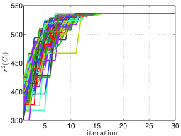
Figure 1: Time evolution of $\mathrm{r}^{2}(\mathrm{\mathcal{C}}_{i}(t))$, $i\in\{1,\dots,N\}$.

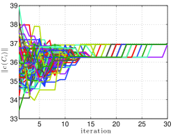
Figure 2: Time evolution of $\|\mathrm{c}(\mathrm{\mathcal{C}}_{i}(t))\|$, $i\in\{1,\dots,N\}$.

VI Conclusions

In this paper we have proposed a distributed algorithm to solve a special class of quadratic programs that models several classification problems. The proposed algorithm handles problems in which not only the number of input data is large, but furthermore their dimension is big. The resulting learning area is known as big-data classification. We have proposed a distributed optimization algorithm that computes an approximate solution of the global problem. Specifically, for any chosen tolerance $\epsilon$, each local node needs to store only $\left\lceil\frac{1}{\epsilon}\right\rceil$ active constraints, which represent a solution for the global quadratic program up to a relative tolerance $\epsilon$. Future research developments include the extension of the algorithmic idea, based on core-sets, to other big-data optimization problems.

References

- [1] V. Cevher, S. Becker, and M. Schmidt, “Convex optimization for big data: Scalable, randomized, and parallel algorithms for big data analytics,” IEEE Signal Processing Magazine, vol. 31, no. 5, pp. 32–43, 2014.
- [2] F. Facchinei, G. Scutari, and S. Sagratella, “Parallel selective algorithms for nonconvex big data optimization,” IEEE Transactions on Signal Processing, vol. 63, no. 7, pp. 1874–1889, 2015.
- [3] K. Slavakis and G. B. Giannakis, “Online dictionary learning from big data using accelerated stochastic approximation algorithms,” in 2014 IEEE International Conference on Acoustics, Speech and Signal Processing (ICASSP), 2014, pp. 16–20.
- [4] Y. Lu, V. Roychowdhury, and L. Vandenberghe, “Distributed parallel support vector machines in strongly connected networks,” IEEE Transactions on Neural Networks, vol. 19, no. 7, pp. 1167–1178, 2008.
- [5] P. A. Forero, A. Cano, and G. B. Giannakis, “Consensus-based distributed support vector machines,” Journal of Machine Learning Research, vol. 11, pp. 1663–1707, 2010.
- [6] S. Lee and A. Nedic, “Drsvm: Distributed random projection algorithms for svms,” in IEEE Conf. on Decision and Control, 2012, pp. 5286–5291.
- [7] S. Boyd, N. Parikh, E. Chu, B. Peleato, and J. Eckstein, “Distributed optimization and statistical learning via the alternating direction method of multipliers,” Foundations and Trends® in Machine Learning, vol. 3, no. 1, pp. 1–122, 2011.
- [8] D. Varagnolo, S. Del Favero, F. Dinuzzo, L. Schenato, and G. Pillonetto, “Finding potential support vectors in separable classification problems,” IEEE Transactions on Neural Networks and Learning Systems, vol. 24, no. 11, pp. 1799–1813, 2013.
- [9] G. Notarstefano and F. Bullo, “Distributed abstract optimization via constraints consensus: Theory and applications,” IEEE Transactions on Automatic Control, vol. 56, no. 10, pp. 2247–2261, October 2011.
- [10] M. Bādoiu, S. Har-Peled, and P. Indyk, “Approximate clustering via core-sets,” in Proceedings of the thiry-fourth annual ACM symposium on Theory of computing, 2002, pp. 250–257.
- [11] M. Badoiu and K. L. Clarkson, “Optimal core-sets for balls,” Comput. Geom., vol. 40, no. 1, pp. 14–22, 2008.
- [12] I. W. Tsang, J. T. Kwok, and P.-M. Cheung, “Core vector machines: Fast svm training on very large data sets,” in Journal of Machine Learning Research, 2005, pp. 363–392.
- [13] S. Lodi, R. Nanculef, and C. Sartori, “Single-pass distributed learning of multi-class svms using core-sets,” in Proceedings of the 2010 SIAM International Conference on Data Mining, 2010, pp. 257–268.
- [14] S. S. Keerthi, S. K. Shevade, C. Bhattacharyya, and K. R. Murthy, “A fast iterative nearest point algorithm for support vector machine classifier design,” IEEE Transactions on Neural Networks, vol. 11, no. 1, pp. 124–136, 2000.
- [15] C. Cortes and V. Vapnik, “Support-vector networks,” Machine Learning, vol. 20, pp. 273–297, 1995.