Optimal digital dynamical decoupling for general decoherence via Walsh modulation

Abstract

We provide a general framework for constructing digital dynamical decoupling sequences based on Walsh modulation — applicable to arbitrary qubit decoherence scenarios. By establishing equivalence between decoupling design based on Walsh functions and on concatenated projections, we identify a family of optimal Walsh sequences, which can be exponentially more efficient, in terms of the required total pulse number, for fixed cancellation order, than known digital sequences based on concatenated design. Optimal sequences for a given cancellation order are highly non-unique — their performance depending sensitively on the control path. We provide an analytic upper bound to the achievable decoupling error, and show how sequences within the optimal Walsh family can substantially outperform concatenated decoupling, while respecting realistic timing constraints. We validate these conclusions by numerically computing the average fidelity in a toy model capturing the essential feature of hyperfine-induced decoherence in a quantum dot.

Dynamical decoupling (DD) techniques, based on open-loop quantum control, provide an effective strategy to reduce decoherence from temporally correlated noise processes in realistic quantum information processing platforms dd ; D. A. Lidar and T. A. Brun (2013) (eds.). In its simplest form, DD coherently averages out the unwanted system-environment interaction through the application of tailored sequences of (ideally, instantaneous) pulses, whose net action on the system translates, in the frequency domain, into a high-pass noise filter A. G. Kofman and G. Kurizki (2004); Green et al. (2013); Paz-Silva and Viola (2014); Soare et al. (2014). To date, the most efficient DD schemes known for generic error models — notably, Uhrig DD Uhrig (2007) and quadratic DD West et al. (2010) for pure dephasing and general decoherence on a single qubit — involve pulse sequences with irrational pulse timing rem . However, consideration of practical constraints highlights crucial advantages of digital DD, whereby all pulse separations are integer multiples of an experimentally restricted minimum time interval. Irrationally-timed DD sequences have been found to be more sensitive to both the form of the spectral cutoff and to inevitable pulse errors Ryan et al. (2010); Xiao et al. (2011); Ajoy et al. (2011), while being less amenable to the additional compensation steps (e.g., via phase-shifts or composite pulses) that are needed to mitigate these errors for arbitrary input states Souza et al. (2012); Wang et al. (2012); Farfurnik et al. (2015); gen . Even in situations where pulse imperfections are unimportant, digital DD sequences are highly compatible with hardware constraints stemming from digital sequencing circuitry and clocking, which makes them attractive in terms of minimizing sequencing complexity, as ultimately demanded for large-scale implementations.

Control modulation based on Walsh functions Beauchamp (1975), has been proposed as a unifying approach for generating digital-efficient protocols, for both dynamically corrected quantum storage and gates Hayes et al. (2011, 2012); Ball and Biercuk (2015); Khodjasteh et al. (2013). Walsh DD (WDD) has been shown to naturally incorporate existing digital sequences as special instances (including concatenated DD for both single- and multi-axis decoherence cdd ), and to provide a restricted search space for numerical sequence optimization and analytic performance analysis under finite timing resources. For dephasing noise on a qubit, concatenated DD sequences based on single-axis control are provably optimal, among the Walsh suite, in the sense of guaranteeing a desired order of error suppression with minimum total pulse number Hayes et al. (2011).

In this work, we identify optimal single-qubit WDD sequences capable of canceling out the simultaneous dephasing and relaxation effects that arise from arbitrary environmental couplings. The key step is to generalize existing sequence constructions of WDD based on multi-axis control, and establish formal equivalence of the resulting general WDD formalism with the concatenated-projection DD (CPDD) approach proposed in Ref. Qi and Dowling (2015). By leveraging this equivalence, we explicitly characterize the error-suppression capabilities of any general WDD sequence, along with its complexity in terms of the required control time slots. We show that, unlike in the dephasing scenario, concatenated DD is no longer optimal, and identify a large family of optimal WDD (OWDD) schemes, whose complexity is exponentially smaller for the same order of suppression. While the performance of different OWDD sequences depends additionally on the specific control path, our analysis indicates that OWDD can substantially improve over existing digital schemes in relevant parameter regimes.

Control-theoretic setting.—We consider a single-qubit system $S$ coupled to an uncontrollable quantum environment (bath) $B$ via an arbitrary interaction, that is, we let the joint evolution in the absence of control to be generated by a Hamiltonian of the form $H\equiv H_{S}\otimes 1\!\!1_{B}+H_{SB}+1\!\!1_{S}\otimes H_{B}$, with $H_{SB}=\sigma_{x}\otimes B_{x}+\sigma_{y}\otimes B_{y}+\sigma_{z}\otimes B_{z}$. Here, $H_{S}$ and $H_{B}\equiv B_{0}$ are, respectively, the internal Hamiltonian for $S$ and $B$ alone, and $\sigma_{u}$, $u\in\{x,y,z\}$, denote qubit Pauli matrices. The bath operators $B_{0},B_{u}$ are assumed to be bounded but otherwise arbitrary (possibly unknown). In what follows, we shall use $\beta\equiv||B_{0}||$ and $J\equiv\max_{u\in\{x,y,z\}}\{||B_{u}||\}$ to quantify the strength of the internal-bath dynamics vs. the system-bath interaction, with $||\cdot||$ being the operator norm.

DD is implemented via a control action on $S$ alone, generated by a control Hamiltonian of the form $H_{c}(t)\otimes 1\!\!1_{B}$. In this work, we consider digital DD sequences consisting of ideal instantaneous $\pi$-pulses along any of the three coordinate axes. Thus, for a sequence specified by pulse timings and control operations $\{t_{j},\sigma_{j}\}$, involving a total of $N$ pulses over a running time $T$, the control Hamiltonian $H_{c}(t)=\frac{\pi}{2}\sum_{j=1}^{N}\sigma_{j}\delta(t-t_{j})$, where we let $t_{0}\equiv 0,t_{N}\equiv T$, and $\sigma_{j}\in\{\sigma_{u}\},\forall j$. Crucially, the digital constraint mandates that all inter-pulse separations obey $t_{j}-t_{j-1}\equiv n_{j}\tau_{0}$, with $n_{j}\in\mathbb{N}$, with the minimum pulse interval $\tau_{0}>0$ determined by hardware limitations. Another convenient representation we shall use for the above sequence is $P_{N}\mathtt{f}_{n_{N}\tau_{0}}\ldots P_{2}\mathtt{f}_{n_{2}\tau_{0}}P_{1}\mathtt{f}_{n_{1}\tau_{0}}$, where the $P_{j}\in\{X,Y,Z\}$ represent different $\pi$ pulses and $\mathtt{f}_{n_{j}\tau_{0}}$ denotes free evolution between $P_{j-1}$ and $P_{j}$.

Since the DD objective is to achieve an identity gate on $S$, all the evolution induced by $H$ contributes to unwanted error dynamics dcg , whereby $H\equiv H_{e}$. Let $U_{c}(t)\equiv\mathcal{T}\exp[-i\int_{0}^{t}H_{c}(t^{\prime})dt^{\prime}]$ be the control propagator, with $\hbar=1$ and $\mathcal{T}$ denoting time-ordering. The effect of $H_{e}$ may be isolated by expressing the propagator $U(T)$, for evolution under $H(t)\equiv H_{e}+H_{c}(t)$ over time $T$, as $U(T)=U_{c}(T)\,\mathcal{T}\exp[-i\int_{0}^{t}\tilde{H}_{e}(t^{\prime})dt^{\prime}]\equiv e^{-i\Omega_{e}(T)}$, where $U_{c}(T)=1\!\!1_{S}$ for DD. $\tilde{H}_{e}(t)=U_{c}^{\dagger}(t)H_{e}U_{c}(t)$ describes evolution in the toggling frame associated to $H_{c}(t)$, and $\Omega_{e}(T)$ defines the error action operator dcg . The norm of $\Omega_{e}(T)$, up to pure-bath terms that do not enter the reduced dynamics, quantifies the achievable error per gate (EPG). Specifically, $\Omega_{e}(T)$ and the associate effective Hamiltonian may be obtained via a perturbative Magnus expansion, $\Omega_{e}(T)\equiv[H_{SB}^{\text{eff}}(T)+H_{B}^{\text{eff}}(T)]T=\exp[\sum_{m=1}^{\infty}\Omega_{e}^{(m)}(T)]$, where $\Omega_{e}^{(m)}(T)$ is a time-ordered integral involving $m^{\text{th}}$-order nested commutators, and $||H||T<\pi$ suffices for (absolute) convergence Blanes et al. (2009). The DD performance in the time domain is then characterized by the order of error suppression (cancellation order, CO), determined by the leading correction mixing $S$ and $B$ in $\Omega_{e}(T)$ dd ; Paz-Silva and Viola (2014). That is, $\text{EPG}\equiv||\text{mod}_{B}(\Omega_{e}(T))||=||TH_{SB}^{\text{eff}}(T)||={\mathcal{O}}(T^{\alpha+1})$ for a protocol with $\text{CO}=\alpha$.

Walsh vs. concatenated-projection DD formalism.—The Walsh functions are a well-known family of binary-valued piecewise-constant functions orthonormal over $[0,1]$, which may be naturally employed to describe digital DD sequences Beauchamp (1975); Hayes et al. (2011). For dephasing noise, single-axis control via $\pi$-pulses around (say) the $x$-axis suffices in the ideal case, resulting in a control propagator of the form $U_{c}(t)\equiv\sigma_{x}^{[x(t)+1]/2}$, where the control switching function $x(t)$ toggles between the values $\pm 1$ at instants corresponding to the applied pulse timings. Let the Walsh function of Paley order $n$ be defined as

$$W_{n}(x)\equiv\prod_{j=1}^{m}R_{j}(x)^{b_{j}},\quad x\in[0,1],$$

where $\{b_{j}\}$ is the binary representation of $n$, namely $n=\sum_{j=1}^{m}b_{j}2^{j-1}$, and $R_{j}(x)\equiv\text{sgn}[\sin(2^{j}\pi x)]$ is the Rademacher function, which switches between $\pm 1$ with frequency $2^{j-1}$. A WDD_n sequence is then defined as the pulse sequence with switching function $x(t)=-W_{n}(t/T)$, $t\in[0,T].$ If $r\equiv\sum_{m}b_{m}$ is the Hamming weight of $n$ (hence the number of Rademacher functions used to construct $W_{n}(x)$), the corresponding WDD_n protocol achieves $\text{CO}=r$ Hayes et al. (2011) .

For a single qubit exposed to multi-axis decoherence, Ref. Hayes et al. (2011) also defines two-axis WDD protocols by allowing for the control propagator $U_{c}(t)$ to involve two switching functions, say, for $\pi$-pulses along the $x$ and $y$ directions, with the form $x(t)=R_{j_{1}}R_{j_{3}}\ldots R_{j_{2r-1}}$, $y(t)=R_{j_{2}}R_{j_{4}}\ldots R_{j_{2r}}$. In this way, for $n=4^{r}-1$, the resulting WDD_n protocol reproduces concatenated DD (CDD) of level $r$, again achieving $\text{CO}=r$ for this general error model cdd .

A different approach to digital DD design is provided by CPDD Qi and Dowling (2015), whereby pulse sequences are built by concatenating projection sequences. There are four such sequences, $\mathtt{p}_{0}\equiv I\mathtt{f}_{\tau_{0}}I\mathtt{f}_{\tau_{0}}$, $\mathtt{p}_{x}\equiv X\mathtt{f}_{\tau_{0}}X\mathtt{f}_{\tau_{0}}$, and similarly for $\mathtt{p}_{y}$ and $\mathtt{p}_{z}$. Applying $\mathtt{p}_{u}$, with $u\in\{x,y,z\}$, suppresses the interaction along perpendicular directions, to the first order, that is, with corresponding $\text{EPG}=\mathcal{O}(\tau_{0}^{2}||H||^{2})$ pro . Given two pulse sequences $A$ and $B$, their concatenation may be defined as $A[B]\equiv P^{A}_{N_{A}}(B)\dots P^{A}_{2}(B)P^{A}_{1}$. The new pulse sequence constructed in this way inherits the suppression capabilities from each of the original pulse sequences. Concatenating a pulse sequence with $\mathtt{p_{0}}$ corresponds to simply repeating the sequence twice. A CPDD_s sequence is then specified by an ordered string $s\equiv s_{m}s_{m-1}\ldots s_{1}$, with $s_{j}\in\{0,x,y,z\}$, with each symbol labeling a projection sequence. To construct the corresponding pulse sequence, projection sequences are concatenated according to the specified string, namely, $\text{CPDD}_{s}\equiv\mathtt{p}_{s_{1}}[\ldots[\mathtt{p}_{s_{m-1}}[\mathtt{p}_{s_{m}}]]].$ For example, in this notation CDD${}_{r}=\text{CPDD}_{(xy)^{r}}$.

General WDD.—Our first result is a generalization of multi-axis WDD beyond the existing one. Unlike the construction in Hayes et al. (2011), we start by expressing the control propagator in terms of three distinct switching functions:

$$U_{c}(t)=\sigma_{x}^{[x(t)+1]/2}\sigma_{y}^{[y(t)+1]/2}\sigma_{z}^{[z(t)+1]/2}.$$ (1)

We define general WDD (GWDD) sequences as follows:

Definition. A GWDD${}_{\vec{n}}$ sequence is specified by an integer vector consisting of three Paley orders, $\vec{n}\equiv(n_{x},n_{y},n_{z}),$ subject to the constraint $\sum_{u=x,y,z}b^{u}_{j}\leq 1$, $1\leq j\leq m_{u}$. Here, $b^{u}_{j}$ is the $j$th digit in the binary representation of $n_{u}$, where $n_{u}=\sum_{j=1}^{m_{u}}b_{j}^{u}2^{j-1}$. The switching function for control along direction $u$ in Eq. (1) is

$$u(t)=-\text{WDD}_{n_{u}}(t/T)=\prod_{j=1}^{m}R_{j}^{u}(t/T)^{b_{j}^{u}},\;t\in[0,T],$$ (2)

with $m\equiv\max\{m_{x},m_{y},m_{z}\}$ and $b_{j}^{u}\equiv 0$ for $m_{u}<j\leq m$.

Since any $\pi$-pulse can be obtained as the product of two $\pi$-pulses along orthogonal directions, the constraint on the coefficients $b_{j}^{u}$ is necessary to avoid redundant sequences, by allowing at most one non-zero digit among all three digits at each binary location. Clearly, the above definition recovers the one in Refs. Hayes et al. (2011); Ball and Biercuk (2015), where a single integer suffices to specify a two-axis WDD_n, due to the assumed particular structure. For instance, $r^{\text{th}}$-order CDD corresponds to a GWDD${}_{\vec{n}}$, with $\vec{n}=(2(4^{r}-1)/(4-1),(4^{r}-1)/(4-1),0)$, with the single above-mentioned Paley order $n=4^{r}-1$ being the sum of three Paley orders in our definition.

Crucially, the above GWDD definition is instrumental to both establish equivalence with the CPDD formalism, and uncover optimal GWDD sequences not accounted for otherwise. To demonstrate the equivalence, note that each non-zero digit $b_{j}^{u}$, in the binary representation of $n_{u}$ in a GWDD sequence, may be associated to a projection $\mathtt{p}_{u}$ in the equivalent CPDD sequence. When $b_{j}^{u}=0$ for all $u\in\{x,y,z\}$, we have an identity projection $\mathtt{p}_{0}$ in CPDD. Explicitly, the following conversion rules hold:

(i) CPDD-to-GWDD. Given a CPDD_s with $s=s_{m}s_{m-1}\ldots s_{1}$, calculate $n_{u}=\sum_{j=1}^{m}b^{u}_{j}2^{j-1}$ for $u\in\{x,y,z\}$, where $b_{j}^{u}=1$ if $s_{j}=u$, otherwise $b_{j}^{\mu}=0$. The corresponding GWDD sequence is GWDD${}_{n_{x},n_{y},n_{z}}$.

(ii) GWDD-to-CPDD. Given a GWDD${}_{n_{x},n_{y},n_{z}}$, first convert each Paley order to its binary representation, $n_{u}=(b_{m_{u}}^{\mu}b_{m_{u}-1}^{\mu}\ldots b_{1}^{u})_{2}$. Second, leftpad the binary representations with zeros so that they all have the same length $m$. For the $j$th digit and $u\in\{x,y,z\}$, set $s_{j}=u$ if $b_{j}^{u}=1$; else, if all $b_{j}^{u}=0$, set $s_{j}=0$. The corresponding CPDD sequence is CPDD_s with $s=s_{m}s_{m-1}\ldots s_{1}$.

The resulting correspondence is illustrated in Table 1 for single-axis sequences. For multi-axis control, we use the so-called GA_8r sequences as an example. The latter is obtained from concatenation of a basic six-pulse, $2^{\text{nd}}$-order GA₈ sequence, $I\mathtt{f}X\mathtt{f}Y\mathtt{f}X\mathtt{f}I\mathtt{f}X\mathtt{f}Y\mathtt{f}X\mathtt{f}$, found by a genetic search algorithm in Ref. Quiroz and Lidar (2013). In the CPDD framework, GA_8r = CPDD${}_{(zyx)^{r}}$. By using the above rules, we have $n_{x}=(100\ldots 100)_{2}$, $n_{y}=(010\ldots 010)_{2}$, $n_{z}=(001\ldots 001)_{2}$. Accordingly, the corresponding GWDD sequence is GWDD${}_{\vec{n}}$, where $\vec{n}$ is given by $\vec{n}=(4(1-2^{3r})/(1-2^{3}),2(1-2^{3r})/(1-2^{3}),(1-2^{3r})/(1-2^{3}))$.

WDDn	CPDDs
WDD0	CPDD0 = p0
WDD1	CPDDx = px
WDD2 = WDD10	CPDDx0 = p0[px]
WDD3 = WDD11	CPDDxx = px[px]
WDD4 = WDD100	CPDDx00 = p0[p0[px]]

Table 1: Equivalence between single-axis WDD and CPDD.

The equivalence with the CPDD formalism makes it possible to easily obtain the CO of an arbitrary GWDD sequence. As shown in Ref. Qi and Dowling (2015), the CO of CPDD is given by $\alpha=\min\{r_{y}+r_{z},r_{x}+r_{z},r_{x}+r_{y}\},$ where $r_{u}$ is the number of projections along the $u$-axis. From the above rules, we see that each such projection implies a non-zero bit in the binary representation of the corresponding Paley order. Therefore, the CO of GWDD is still given by the above equation, but with $\{r_{u}=\sum_{j}b_{j}^{u}\}$ now being Hamming weights. It follows that GWDD/CPDD sequences with the same CO are highly non-unique: permuting the order of projections will produce a different GWDD sequence, but leave the CO unchanged. Accordingly, we may think of GWDD sequences specified by $(r_{{\cal P}(x)},r_{{\cal P}(y)},r_{{\cal P}(z)})$, where ${\cal P}\in{\cal S}_{3}$ is any permutation, as forming an equivalence class with respect to CO.

	OWDD			CDD
CO	($n_{x},n_{y},n_{z}$)	$N_{T}$	$N$	($n_{x},n_{y},n_{z}$)	$N_{T}$	$N$
1	(2,1,0)	4	4	(2,1,0)	4	4
2	(4,2,1)	8	6	(10,5,0)	16	14
3	(18,5,4)	32	32	(42,21,0)	64	60
4	(36,18,9)	64	42	(170,85,0)	256	238

Table 2: Number of control time slots and applied pulses for OWDD vs. CDD. Taking either $N_{T}$ or $N$ does not change the optimality of OWDD, as their differences are negligible compared to the exponential saving.

Optimal Walsh DD.—In the presence of a realistic constraint, $\tau_{0}>0$, achieving higher CO comes at the price of either increasing the total number of pulses $N$ for fixed storage time $T$ — until the maximum CO compatible with the constraints is accommodated; or of increasing both $N$ and $T$ — until perturbative error suppression breaks down and, again, a maximum CO is reached beyond which no further improvement occur Khodjasteh et al. (2013). This motivates defining optimal WDD (OWDD) sequences by demanding that they guarantee a desired CO with minimum pulse number or, equivalently, minimum number of time slots, $N_{T}$, each slot having duration $\tau_{0}$. Within single-axis WDD, CDD sequences are provably optimal Hayes et al. (2011). However, this is no longer true for multi-axis GWDD. The optimal GWDD can be inferred from the CPDD framework. For $\text{CO}=\alpha$, let $\overline{\alpha}=\pm 1$ denote the parity of $\alpha$. Then, all GWDD${}_{\vec{n}}$ satisfying the following two conditions are optimal and define an equivalence class referred to as OWDD_α:

$$\sum\limits_{u=x,y,z}b_{j}^{u}=1,\quad 1\leq j\leq m,$$ (3)

$$(r_{{\cal P}(x)},r_{{\cal P}(y)},r_{{\cal P}(z)})=\frac{1}{2}\left(\alpha-\overline{\alpha},\alpha+\overline{\alpha},\alpha+\overline{\alpha}\right).$$ (4)

Eq. (3) ensures that the pulse sequence does not expend any pulse on repetition, whilst Eq. (4) gives the Hamming weights (number of projections) needed to suppress decoherence up to the required CO. From the equivalence between CPDD and GWDD, and the analysis in Ref. Qi and Dowling (2015), it follows that OWDD_α uses a number of time slots given by $\log_{2}(N_{T})=\frac{1}{2}\left(3\alpha+\overline{\alpha}\right).$ A comparison between OWDD_α and CDD_α is included in Table 2. If the CO is sufficiently large, OWDD_α is exponentially more efficient than CDD, since $N_{T}^{\text{OWDD}_{\alpha}}/N_{T}^{\text{CDD}_{\alpha}}\approx 2^{\frac{3}{2}\alpha}/2^{2\alpha}=2^{-\alpha/2}.$

Performance analysis.—The EPG provides an appropriate performance measure for control since it upper-bounds the trace-norm distance between the intended and the actual final states of the system, say, $\Delta(\rho_{S}^{0}(T),\rho_{S}(T))$, where $\rho_{S}^{0}(T)=\rho_{S}^{0}(0)\equiv|\psi\rangle\langle\psi|$ for DD Lidar et al. (2008); dcg . That is, $\Delta(\rho_{S}^{0}(T),\rho_{S}(T))\leq||TH_{SB}^{\text{eff}}(T)||$ independently of $\left|\psi\right\rangle$, which in turn allows us to bound experimentally accessible fidelities as $1-\Delta\leq F\leq\sqrt{1-\Delta^{2}}$ (here, $F(\rho,|\psi\rangle\langle\psi|)\equiv\text{tr}\sqrt{\sqrt{\rho}\,|\psi\rangle\langle\psi|\sqrt{\rho}}\,$). An analytical upper bound to the EPG may be derived by leveraging the geometrical picture afforded by CPDD. The basic idea is to observe that, if the error action operator for a sequence CPDD${}_{s_{0}}$ with running time $T_{s_{0}}$ has the form $\Omega_{e}(T_{s_{0}})\equiv T_{s_{0}}[\sum_{u}\sigma_{u}\otimes B_{u}^{s_{0}}+B_{0}^{s_{0}}]$, concatenation with a projection sequence, say, $\mathtt{p}_{x}[\text{CPDD}_{s_{0}}]\equiv\text{CPDD}_{s_{0}x}$, has a simple effect in terms of renormalizing bath operators in the orthogonal directions. Specifically, one finds sup that the resulting error action, $\Omega_{e}(2T_{s_{0}})$, has the same structure as $\Omega_{e}(T_{s_{0}})$, only with new bath operators:

$$||B_{0}^{s_{0}x}|| =||B_{0}^{s_{0}}||,\quad||B_{x}^{s_{0}x}||=||B_{x}^{s_{0}}||,$$ (5a)

$$||B_{y}^{s_{0}x}|| \leq T_{s_{0}}(\beta||B_{y}^{s_{0}}||+||B_{z}^{s_{0}}||\,||B_{x}^{s_{0}}||),$$ (5b)

$$||B_{z}^{s_{0}x}|| \leq T_{s_{0}}(\beta||B_{z}^{s_{0}}||+||B_{y}^{s_{0}}||\,||B_{x}^{s_{0}}||),$$ (5c)

as long as $\beta\gg J$ or $\ll J$, and $\max\{\beta,J\}\tau_{0}\ll 1$. Similar inequalities hold when we concatenate CPDD_s with $\mathtt{p}_{y}$ or $\mathtt{p}_{z}$. Therefore, given an arbitrary GWDD sequence, the desired upper bound may be obtained by first translating it into the equivalent CPDD_s, and then by repeatedly using Eqs. (5) according to the “projection path” specified by $s=s_{m}\ldots s_{1}$, leading to $\text{EPG}\leq T_{s}\sum_{u=x,y,z}||B_{u}^{s}||$.

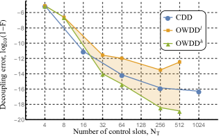
Figure 1: (Color online) Fidelity loss vs. $N_{T}$ for two choices of OWDD_α protocols with same CO and CDD. The shaded area marks the performance spread expected for all OWDD_α protocols in the same equivalence class. A toy model consisting of three bath spins is used, with an initial joint state of the form $\left|\Psi\right\rangle_{SB}\equiv\left|\psi\right\rangle\otimes\left|z_{1}z_{2}z_{3}\right\rangle$, where $\left|\psi\right\rangle$ is a random qubit state and each bath spin is randomly chosen over $z_{i}\in\{0,1\}$. Results are averaged over 500 realizations. We choose parameters $\beta$ = 10kHz, $J=1$MHz, and $\tau_{0}=0.1\mu$s, suitable for qualitatively describing GaAs quantum dots Coish et al. (2006).

Since, in each use of Eqs. (5), the duration of the sequence before concatenation enters explicitly, the EPG of two GWDD sequences with the same number of projections along each direction will still differ depending on the order in which the projections are taken — resulting in different fidelities for the same CO. To illustrate this sensitivity to the control path, we compare two different choices in the same OWDD_α equivalence class with CDD. Let OWDD${}^{{h}}_{\alpha}\equiv$ $\{\text{CPDD}_{xy}$, $\text{CPDD}_{xyz}$, $\text{CPDD}_{xyzxy}$, $\text{CPDD}_{(xyz)^{2}},...\}$, and OWDD${}^{{l}}_{\alpha}\equiv$ $\{\text{CPDD}_{xy}$,$\text{CPDD}_{xyz}$, $\text{CPDD}_{xxyyz}$, $\text{CPDD}_{x^{2}y^{2}z^{2}},...\}$, for $\alpha=1,2,3,4$. Both obey Eqs. (3) and (4) for the same $(r_{x},r_{y},r_{z})$. As detailed in Ref. sup , OWDD${}^{{l\,(h)}}_{\alpha}$ sequences result in comparatively high (low) EPG due to their larger (smaller) prefactor: e.g., at $\text{CO}=3$, one finds $\text{EPG}^{{\text{OWDD}^{h}_{3}}}\leq 5\cdot 2^{5}(\tau_{0}\beta)^{3}JT$ vs. $\text{EPG}^{{\text{OWDD}^{l}_{3}}}\leq 16\cdot 2^{5}(\tau_{0}\beta)^{3}JT$, with $T=2^{5}\tau_{0}$, and the difference further increasing for higher CO. Geometrically, if one visualizes the implemented sequence of projections in terms of a lattice path starting at the origin in $\mathbb{N}^{3}$, OWDD^h maximizes the number of switches in direction as compared to OWDD^l. That avoiding control path repetitions is generally useful in slowing down coherent error build-up, has been emphasized in the context of randomized DD design Santos and Viola (2008), and we conjecture that a similar intuition may be key for further optimizing OWDD against path variations.

We conclude by comparing in Fig. 1 the performance of OWDD and CDD directly in terms of average fidelity loss, by resorting to an exact numerical simulation of a low-dimensional spin-bath model, which mimics the basic features of hyperfine-induced decoherence of an electron spin qubit in a quantum dot de Sousa and Sarma (2003); Coish et al. (2006). The bath operators are $B_{\mu}=\sum_{i\neq j}\sum_{\alpha,\beta}c^{\mu}_{\alpha\beta}(\sigma^{\alpha}_{i}\otimes\sigma^{\beta}_{j})$, where $i,j$ index the bath qubits, $\mu,\alpha,\beta\in\{0,x,y,z\}$, and $c^{\mu}_{\alpha\beta}$ are uniformly random coupling constants in $[0,1]$ . We assume a fixed minimum pulse interval $\tau_{0}=0.1\mu$s. At large $N_{T}$, the performance tends to plateau (or even deteriorate) due to the fact that convergence breaks down for long $T$ (see also Ref. pre ). Remarkably, if OWDD${}_{\alpha}^{h}$ is used, comparable performance to CDD_α is found for smaller $N_{T}$, whereas for same $N_{T}$, the fidelity of OWDD can be higher than the one of CDD by up to two orders of magnitude.

In a realistic scenario, pulse imperfections are an additional important factor in limiting achievable operational fidelities. While we leave the study of realistic control errors to a future separate investigation, it is worth noting that the robust RGA₈ family identified in Quiroz and Lidar (2013) is built by suitably incorporating phase alternation into the even orders of OWDD^h, pointing to an interesting venue for generalization. A characterization of OWDD in terms of control symmetry properties (including “displacement anti-symmetry” as in Paz-Silva et al. (2016)) and a more rigorous understanding of path sensitivity are also well worth pursuing, along with extensions to multi-qubit DD settings.

It is a pleasure to thank Gregory Quiroz, Gerardo Paz-Silva, Kaveh Khodjasteh, Leigh Norris, and Manish Gupta for helpful discussions. LV gratefully acknowledges support from the US Army Research Office under contract No. W911NF-14-1-0682. HQ and JPD are supported by the Air Force Office of Scientific Research, the Army Research Office, the National Science Foundation and the Northrop Grumman Corporation.

Supplementary Material

I Upper bound on EPG for general Walsh DD sequences

In this section, we provide a detailed derivation of Eq. (5), and the upper bound to the EPG quoted in the main text for arbitrary GWDD sequences. Thanks to the equivalence between GWDD and CPDD, we only need to calculate the upper bound for the corresponding CPDD sequence. The geometrical picture of projections makes CPDD the natural framework to use. Specifically, we first show how the norm of the relevant interaction Hamiltonian is renormalized by a single projection sequence. Since every CPDD sequence arises from concatenation of a series of projections, we can then apply the result of a single projection recursively, to establish the desired upper bound.

I.1 Bath renormalization by a single projection

Consider first the effect of a single projection sequence, say $\mathtt{p_{x}}$. The resulting toggling-frame error Hamiltonian is

$$\tilde{H}_{e}(t)=\begin{cases}H,~{}~{}0\leq t\leq\tau_{0},\\ XHX,~{}~{}\tau_{0}\leq t\leq 2\tau_{0}.\end{cases}$$ (6)

Since $\tilde{H}_{e}(t)$ is a piece-wise constant function, the first three orders of the Magnus series expansion may be easily computed as

$$\Omega_{e}^{(1)} = \tau_{0}(H+XHX),$$

$$\Omega_{e}^{(2)} = -\frac{i}{2}\tau_{0}^{2}[H,XHX],$$

$$\Omega_{e}^{(3)} = \frac{1}{3!}\tau_{0}^{3}[XHX[H,XHX]].$$

By using the explicit form of $H=\sum_{\mu=0,x,y,z}\sigma_{\mu}\otimes B_{\mu}$ given in the main text, together with Eq. (6) above, the first two contributions become

$$\Omega_{e}^{(1)} = 2\tau_{0}(1\!\!1\otimes B_{0}+B_{x}\otimes X),$$ (7)

$$\Omega_{e}^{(2)} = Y\otimes\tau_{0}^{2}(i[B_{0},B_{y}]+\{B_{z},B_{x}\})+Z\otimes\tau_{0}^{2}(i[B_{0},B_{z}]+\{B_{y},B_{x}\}),$$ (8)

with a corresponding norm

$$||\Omega_{e}^{(1)}||=O(\tau_{0}(\beta+J)),\quad\quad||\Omega_{e}^{(2)}||=O(\tau_{0}^{2}J(\beta+J)).$$

Although the Magnus expansion converges as long as $||H||T<\pi$, care is needed in discarding higher-order terms. The norm of the third-order term is found to be

$$||\Omega_{e}^{(3)}||=O(\tau_{0}^{3}\beta J(\beta+J))+O(\tau_{0}^{3}J^{3}).$$ (9)

Accordingly, it is not possible in general to ignore this contribution as it is not clear which term in Eq. (9) dominates. Following the analysis in K. Khodjasteh and D. A. Lidar, Phys. Rev. A 75, 062310 (2007), we proceed by addressing separately two limiting regimes:

$\bullet$ When $J\ll\beta$, we have $||\Omega_{e}^{(1)}||=O(\tau_{0}\beta)$, $||\Omega_{2}^{(2)}||=O(\tau_{0}\beta J)$ and $||\Omega_{e}^{(i)}||=O(\tau_{0}^{i}\beta^{i-1}J).$ Therefore, we have

$$||\Omega_{e}^{(1)}||<||\Omega_{e}^{(2)}||\ll||\Omega_{e}^{(i\geq 3)}||,$$ (10)

as long as the condition $\beta\tau_{0}\ll 1$ is obeyed.

$\bullet$ When $J\gg\beta$, we have $||\Omega_{e}^{(i)}||=O(\tau_{0}^{i}J^{i})$. Thus, the same relation given in Eq. (10) holds, as long as $J\tau_{0}\ll 1$.

In summary, when $J\gg\beta$ or $J\ll\beta$, provided that $\tau_{0}||H||\ll 1$, it suffices to retain the first two orders of the Magnus expansion, giving an approximate expression for the error action operator as

$$\Omega_{e}(2\tau_{0})\approx\Omega^{(1)}(2\tau_{0})+\Omega^{(2)}(2\tau_{0})\equiv 2\tau_{0}\bar{H}^{x}=2\tau_{0}\sum_{\mu=0,x,y,z}\sigma_{\mu}\otimes B^{x}_{\mu},$$

where in the last equality we have defined the average Hamilton associated with $\mathtt{p}_{x}$ and the relevant renormalized bath operators. From Eqs. (7) and (8), we can read them off as

$$B_{0}^{x} = B_{0},$$

$$B_{x}^{x} = B_{x},$$

$$B_{y}^{x} = \frac{\tau_{0}}{2}(i[B_{0},B_{y}]+\{B_{z},B_{x}\}),$$

$$B_{z}^{x} = \frac{\tau_{0}}{2}(i[B_{0},B_{z}]+\{B_{y},B_{x}\}).$$

Similar equations hold for projections along the $y$ or $z$ directions. When the strength of the system-bath interaction and the pure bath dynamics are of the same order of magnitude, $J\sim\beta$, the calculation depends on the specific value of $J$ and $\beta$, and no general analytic error bound may be established. From now on, we thus assume that the system is in either of the two regimes mentioned above.

I.2 Bath renormalization in an arbitrary CPDD sequence

Consider a CPDD sequence specified by an ordered string $s_{0}$, with total running time $T_{s_{0}}$. Let the relevant effective Hamiltonian be denoted by $\bar{H}^{s_{0}}$. We now construct a new CPDD sequence by concatenating it with a projection sequence, say, $\mathtt{p}_{x}$, obtaining a CPDD${}_{s_{0}x}$, whose renormalized effective Hamiltonian $\bar{H}^{s_{0}x}$ we wish to determine.

The evolution propagator of the system under the control of CPDD${}_{s_{0}x}$ is

$$X(e^{-i\bar{H}^{s_{0}}T_{s_{0}}})X(e^{-i\bar{H}^{s_{0}}T_{s_{0}}})=e^{-iXe^{-i\bar{H}^{s_{0}}T_{s_{0}}}X}e^{-ie^{-i\bar{H}^{s_{0}}T_{s_{0}}}}.$$

Therefore, the toggling-frame error Hamiltonian $\bar{H}^{{s_{0}}x}(t)$ is still a piece-wise constant function,

$$\bar{H}^{{s_{0}}x}(t)=\begin{cases}\bar{H}^{{s_{0}}}~{}~{},0\leq t\leq T_{s_{0}},\\ X\bar{H}^{s_{0}}X~{}~{},T_{s_{0}}\leq t\leq 2T_{s_{0}},\end{cases}$$

which makes it possible to use the same analysis used in the previous section. Accordingly, in the two regimes where $J\ll\beta$ or $J\gg\beta$, the renormalized bath operators are given by

$$B_{0}^{{s_{0}}x} = B_{0}^{{s_{0}}},$$

$$B_{x}^{{s_{0}}x} = B_{x}^{{s_{0}}},$$

$$B_{y}^{{s_{0}}x} = \frac{T_{s_{0}}}{2}\left(i[B_{0},B_{y}^{s_{0}}]+\{B_{z}^{s_{0}},B_{x}^{s_{0}}\}\right),$$

$$B_{z}^{{s_{0}}x} = \frac{T_{s_{0}}}{2}\left(i[B_{0},B_{z}^{s_{0}}]+\{B_{y}^{s_{0}},B_{x}^{s_{0}}\}\right),$$ (11)

where $B_{\mu}^{s_{0}},\mu\in\{0,x,y,z\}$ are the effective bath operators of CPDD${}_{s_{0}}$. As we can see, $\mathtt{p}_{x}$ leaves $B^{s_{0}}_{x}$ unchanged, but renormalizes $B^{s_{0}}_{y}$ and $B^{s_{0}}_{z}$ to the next order. Similar renormalization relations hold for $\mathtt{p}_{y}$ and $\mathtt{p}_{z}$.

Eqs. (5) in the main text follows from applying standard operator-norm inequalities to the renormalized bath operators in Eq. (11), in particular, $||[A,B]||\leq 2||A||\,||B||,$ $\||A+B||\leq||A||+||B||,$ and $||AB||\leq||A||\,||B||.$ Along with the definition of the EPG, this yields the desired result for CPDD_s,

$$\text{EPG}\leq T_{s}\sum_{u=x,y,z}||B_{u}^{s}||.$$

II Control path sensitivity

As remarked in the main text, any permutation of the order of concatenation in building CPDD sequences will leave the CO invariant. We expect that pulse sequence with a different control path will give different performance, since the EPG (or fidelity) do not solely depends on the CO. In the context of GWDD, control path sensitivity may be understood by comparing the upper bounds of the EPG generated by different control paths. As shown by Eq. (5) in the main text, the EPG of CPDD sequences generated by permutations of a sequence $s$, have the same scaling behavior on $\tau_{0}$, but produce different prefactors. In this section, we first present a concrete example to demonstrate how the information about the control path is “encoded” into the prefactors of the relevant EPG. We then provide a more convenient way to calculate the prefactor for any GWDD/CPDD sequences, whereby we also derive the relevant prefactors for the OWDD${}^{l\,(h)}$ sequences analyzed in the main text.

II.1 Switches in the control path are good for error suppression

The simplest non-trivial example we may consider is to compare CDD${}_{2}=\text{CPDD}_{xyxy}$ with the CPDD sequence generated by a permutation of $xyxy$, denoted by $\overline{\text{CDD}}_{2}=\text{CPDD}_{xxyy}$. To simplify the calculation and to focus on prefactor, we assume the regime $\beta\gg J$. Applying the renormalization given in Eq. (5) repeatedly, we have for CDD₂

$$||B_{x}^{xyxy}|| \leq 2^{3}\cdot 2^{1}\tau_{0}^{2}\beta^{2}J,$$

$$||B_{y}^{xyxy}|| \leq 2^{2}\cdot 2^{0}\tau_{0}^{2}\beta^{2}J,$$

where at each step we only keep the leading-order terms. The bound for $||B_{z}||$ is always higher order than the other two directions since both $\mathtt{p}_{x}$ and $\mathtt{p}_{y}$ suppress $B_{z}$. In the above equations we also see explicitly how the prefactors are accumulated. Similarly, for $\overline{\text{CDD}}_{2}$, we apply Eq.(5) repeatedly but with a different order, obtaining

$$||B_{x}^{xxyy}|| \leq 2^{3}\cdot 2^{2}\tau_{0}^{2}\beta^{2}J,$$

$$||B_{y}^{xxyy}|| \leq 2^{1}\cdot 2^{0}\tau_{0}^{2}\beta^{2}J.$$

As we can see, the upper bounds of CDD₂ and $\overline{\text{CDD}}_{2}$ have the same scaling over $\tau_{0}$, consistent with the fact that both of them achieve $\text{CO}=2$. However, CDD₂ has a smaller prefactor than $\overline{\text{CDD}}_{2}$:

$$\text{EPG}^{xyxy} \leq 20\,\tau_{0}^{2}\beta^{2}JT$$

$$\text{EPG}^{xxyy} \leq 34\,\tau_{0}^{2}\beta^{2}JT.$$

This can be qualitatively explained as follows. When $\mathtt{p}_{x}$ is applied, the upper bound for $||B_{y}||$ will start to accumulate a prefactor. If we continue applying $\mathtt{p}_{x}$, like in $\overline{\text{CDD}}$, the prefactor for $||B_{y}||$ will grow exponentially since the length of the sequence is exponentially increasing. However, if the direction of the projection sequence is changed at a certain point, say to $\mathtt{p}_{y}$, then the prefactor for $||B_{y}||$ will stop increasing. Therefore, CPDD sequences, with a large number of switches in the direction of the corresponding projections, tend to have lower error and better performance. For sufficiently large CO we may write

$$\text{EPG}^{\text{CDD}_{\alpha}} \leq 2^{\alpha^{2}}(\tau_{0}\beta)^{\alpha}JT,$$

$$\text{EPG}^{\overline{\text{CDD}}_{\alpha}} \leq 2^{\frac{1}{2}(3\alpha^{2}-\alpha)}(\tau_{0}\beta)^{\alpha}JT.$$

The above conclusions remain unchanged if we work in the opposite regime, $\beta\ll J$, since the prefactor only depends on the order of concatenations.

II.2 Calculating prefactors for GWDD/CPDD sequences

The method we described above to calculate the prefactors for GWDD sequences relies upon the geometric picture of CPDD. However, the calculation is tedious, especially for long pulse sequences. Here, we present an alternative method to directly calculate the prefactor for any GWDD/CPDD sequence.

Consider a pulse sequence CPDD_s. Then:

1. Define $s^{\prime}$ to be the sequence of letters in the reverse order of $s$, namely, $s^{\prime}\equiv s_{1}\ldots s_{m}$. Construct a $3\times|s|$ matrix, denoted by $\mathcal{L}$, according to the following rule:

   $$\mathcal{L}_{\mu j}\equiv\begin{cases}1,~{}\text{if}~{}s_{j}=\mu~{}\\ 0,~{}\text{otherwise}\end{cases}~{}.$$ (12)

   where we use $\mu\in\{x,y,z\}$ to label the $1^{\text{st}}$, the $2^{\text{nd}}$ and the $3^{\text{rd}}$ row of $\mathcal{L}$.

2. The prefactor in the upper bound on $||B_{\mu}^{s}||$ is then given by

   $$\prod_{\begin{subarray}{c}j=1\\ \bar{\mathcal{L}}_{\mu j}\neq 0\end{subarray}}^{|s|}\bar{\mathcal{L}}_{\mu j}2^{j-1}~{},$$ (13)

   where the matrix $\bar{\mathcal{L}}$ is the logical negation of $\mathcal{L}$.

3. If we assume $\beta\gg J$ and ignore higher-order contributions, we have the following upper bound

   $$||B_{\mu}^{s}||\leq\left(\prod_{\begin{subarray}{c}j=1\\ \bar{\mathcal{L}}_{\mu j}\neq 0\end{subarray}}^{|s|}\bar{\mathcal{L}}_{\mu j}2^{j-1}\right)(\tau_{0}\beta)^{\sum_{k=1}^{|s|}\bar{\mathcal{L}}_{\mu k}}J~{}.$$ (14)

We illustrate the above procedure by considering a simple example, namely, the second level of OWDD sequences, CPDD_xyz. From the definition of CPDD sequence, $s^{\prime}=xyz$, hence the matrix $\mathcal{L}$ is given by

$$\blockarray{cccccc}s^{\prime}&xyz\\ \block{ccc[ccc]}x100\\ y010\\ z001\\ ~{}.$$

Here, the row indexes represent different directions while the column indexes are specified by $s^{\prime}$. Applying Eq. (13) and Eq. (14), and assuming $\beta\gg J$, we get

$$||B_{x}^{xyz}||\leq 2^{2}\cdot 2^{1}(\tau_{0}\beta)^{2}J,$$

$$||B_{y}^{xyz}||\leq 2^{2}\cdot 2^{0}(\tau_{0}\beta)^{2}J,$$

$$||B_{z}^{xyz}||\leq 2^{1}\cdot 2^{0}(\tau_{0}\beta)^{2}J.$$

II.3 Path sensitivity for optimal Walsh DD sequences

Any GWDD sequence that achieves $\text{CO}=\alpha$, with a number of time slots obeying $\log_{2}(N_{T})=\frac{1}{2}\left(3\alpha+\overline{\alpha}\right)$, as explained in the main text [see also Table II], is an OWDD_α sequence. Although different choices of OWDD use the same number of control time slots for given CO, their performance is different due to the control path sensitivity discussed above. Based on the intuitive argument we described, we expect that OWDD sequences with a larger number of switches will comparatively achieve a lower EPG, hence higher fidelity. With this intuition in mind, we consider OWDD sequences with the maximum number of switches,

$$\text{OWDD}^{h}_{\alpha}\equiv\{\text{CPDD}_{xy},\text{CPDD}_{xyz},\text{CPDD}_{xyzxy},\text{CPDD}_{(xyz)^{2}},\ldots\},$$

as well as sequences where this number is minimized and the lattice-path trajectory has long straight segments:

$$\text{OWDD}^{l}_{\alpha}\equiv\text{CPDD}_{x^{r_{x}}y^{r_{y}}z^{r_{z}}}=\{\text{CPDD}_{xy},\text{CPDD}_{xyz},\text{CPDD}_{xxyyz},\text{CPDD}_{xxyyzz},\ldots\},$$

as also defined in the main text.

The first two orders of OWDD sequences are the same for any choice of OWDD. Thus, in order to illustrate the control path sensitivity, below we explicitly calculate the upper bound of EPG for the next two levels of OWDD^h and OWDD^l, corresponding to $\text{CO}=3,4$, respectively.

To calculate the upper bound for OWDD${}^{h}_{3}$ = CPDD_xyzxy, we first write down the $\mathcal{L}$ matrix according to Eq.(12),

$$\mathcal{L}=\begin{bmatrix}1&0&0&1&0\\ 0&1&0&0&1\\ 0&0&1&0&0\end{bmatrix}~{}.$$ (15)

Calculate its negation $\bar{\mathcal{L}}$ and then the upper bound according to Eq.(14):

$$||B_{x}^{xyzxy}|| \leq 2^{4}\cdot 2^{2}\cdot 2^{1}(\tau_{0}\beta)^{3}J,$$

$$||B_{y}^{xyzxy}|| \leq 2^{3}\cdot 2^{2}\cdot 2^{0}(\tau_{0}\beta)^{3}J,$$

$$||B_{z}^{xyzxy}|| \leq 2^{4}\cdot 2^{3}\cdot 2^{1}\cdot 2^{0}(\tau_{0}\beta)^{4}J.$$

By discarding the higher-order contribution from $||B_{z}||$, we have $\text{EPG}^{\text{OWDD}^{h}_{3}}\leq 5\cdot 2^{5}(\tau_{0}\beta)^{3}JT$, where $T=2^{5}\tau_{0}$. Following the same procedure for OWDD${}^{h}_{4}$, we have

$$||B_{x}^{xyzxyz}|| \leq 2^{5}\cdot 2^{4}\cdot 2^{2}\cdot 2^{1}(\tau_{0}\beta)^{4}J,$$

$$||B_{y}^{xyzxyz}|| \leq 2^{5}\cdot 2^{3}\cdot 2^{2}\cdot 2^{0}(\tau_{0}\beta)^{4}J,$$

$$||B_{z}^{xyzxyz}|| \leq 2^{4}\cdot 2^{3}\cdot 2^{1}\cdot 2^{0}(\tau_{0}\beta)^{4}J,$$

the EPG is dominated by the $x$ direction and we have $\text{EPG}^{\text{OWDD}^{h}_{4}}\leq 2^{12}\,(\tau_{0}\beta)^{4}JT$, with $T=2^{6}\tau_{0}$.

Now we calculate the upper bounds for OWDD${}^{l}_{\alpha}$. To calculate the upper bound of OWDD${}^{l}_{3}$, we write down the $\mathcal{L}$ matrix first, namely,

$$\mathcal{L}=\begin{bmatrix}1&1&0&0&0\\ 0&0&1&1&0\\ 0&0&0&0&1\end{bmatrix}~{}.$$ (16)

Then the upper bounds of bath operators are given by Eq. (14),

$$||B_{x}^{xxyyz}|| \leq 2^{4}\cdot 2^{3}\cdot 2^{2}(\tau_{0}\beta)^{3}J,$$

$$||B_{y}^{xxyyz}|| \leq 2^{4}\cdot 2^{1}\cdot 2^{0}(\tau_{0}\beta)^{3}J,$$

$$||B_{z}^{xxyyz}|| \leq 2^{3}\cdot 2^{2}\cdot 2^{1}\cdot 2^{0}(\tau_{0}\beta)^{4}J.$$

Therefore, $\text{EPG}^{\text{OWDD}^{l}_{3}}\leq 2^{4}\cdot 2^{5}(\tau_{0}\beta)^{3}JT$, with $T=2^{5}\tau_{0}$. Similarly, the upper bounds for OWDD${}_{4}^{l}$ are given by

$$||B_{x}^{xxyyzz}|| \leq 2^{5}\cdot 2^{4}\cdot 2^{3}\cdot 2^{2}(\tau_{0}\beta)^{4}J,$$

$$||B_{y}^{xxyyzz}|| \leq 2^{5}\cdot 2^{4}\cdot 2^{1}\cdot 2^{0}(\tau_{0}\beta)^{4}J,$$

$$||B_{z}^{xxyyzz}|| \leq 2^{3}\cdot 2^{2}\cdot 2^{1}\cdot 2^{0}(\tau_{0}\beta)^{4}J,$$

whereby $\text{EPG}^{\text{OWDD}^{l}_{4}}\leq 2^{14}\,(\tau_{0}\beta)^{4}JT$, with $T=2^{6}\tau_{0}$.

As one can see from the above calculations, at $\text{CO}=3$ the EPG upper bound of OWDD^h is about $3.2$ times smaller than the one for OWDD^l, and becomes four times smaller at $\text{CO}=4$. Therefore, an increasingly larger benefit is expected also in terms of fidelity from using OWDD^h with larger CO.

References

(1)L. Viola and S. Lloyd, Phys. Rev. A 58, 2733 (1998); L. Viola, E. Knill, and S. Lloyd, Phys. Rev. Lett. 82, 2417 (1999).
D. A. Lidar and T. A. Brun (2013) (eds.)D. A. Lidar and T. A.
Brun (eds.), Quantum Error
Correction (Cambridge University Press, 2013).
A. G. Kofman and G. Kurizki (2004)A. G. Kofman and G.
Kurizki, Phys.
Rev. Lett. 93, 130406
(2004).
Green et al. (2013)T. J. Green, J. Sastrawan,
H. Uys, and M. J. Biercuk, New J. Phys. 15, 095004 (2013).
Paz-Silva and Viola (2014)G. A. Paz-Silva and L. Viola, Phys.
Rev. Lett. 113, 250501
(2014).
Soare et al. (2014)A. Soare, H. Ball,
M. C. Jarratt, J. J. McLoughlin, X. Zhen, T. J. Green, and M. J. Biercuk, Nat. Phys. 10, 825 (2014).
Uhrig (2007)G. S. Uhrig, Phys.
Rev. Lett. 98, 100504
(2007).
West et al. (2010)J. R. West, B. H. Fong, and D. A. Lidar, Phys. Rev. Lett. 104, 130501 (2010).
(9)In limiting parameter regimes, irrational
timings may be avoided by incorporating special symmetries into the sequence
design, see Ref. Paz-Silva et al. (2016) for multi-qubit dephasing.
Ryan et al. (2010)C. Ryan, J. Hodges, and D. Cory, Phys. Rev. Lett. 105, 200402 (2010).
Xiao et al. (2011)Z. Xiao, L. He, and W. Wang, Phys. Rev. A 83, 032322 (2011).
Ajoy et al. (2011)A. Ajoy, G. A. Álvarez, and D. Suter, Phys.
Rev. A 83, 032303
(2011).
Souza et al. (2012)A. M. Souza, G. A. Álvarez, and D. Suter, Philos.
T. R. Soc. A 370, 4748
(2012).
Wang et al. (2012)Z.-H. Wang, G. De Lange,
D. Ristè, R. Hanson, and V. Dobrovitski, Phys. Rev. B 85, 155204 (2012).
Farfurnik et al. (2015)D. Farfurnik, A. Jarmola,
L. M. Pham, Z.-H. Wang, V. V. Dobrovitski, R. L. Walsworth, D. Budker, and N. Bar-Gill, Phys. Rev. B 92, 060301 (2015).
(16)G. T. Genov, D. Schraft, N. V. Vitanov, and
T. Halfmann, e-print arXiv:1609.09416.
Beauchamp (1975)K. G. Beauchamp, Walsh Functions and
their Applications, Vol. 3 (Academic Press, 1975).
Hayes et al. (2011)D. Hayes, K. Khodjasteh,
L. Viola, and M. J. Biercuk, Phys. Rev. A 84, 062323 (2011).
Hayes et al. (2012)D. Hayes, S. M. Clark,
S. Debnath, D. Hucul, I. V. Inlek, K. W. Lee, Q. Quraishi, and C. Monroe, Phys. Rev. Lett. 109, 020503 (2012).
Ball and Biercuk (2015)H. Ball and M. J. Biercuk, EPJ
Quantum Tech. 2, 1
(2015).
Khodjasteh et al. (2013)K. Khodjasteh, J. Sastrawan, D. Hayes,
T. J. Green, M. J. Biercuk, and L. Viola, Nat. Commun. 4, 2045 (2013).
(22)K. Khodjasteh and D. A. Lidar, Phys. Rev.
Lett. 95, 180501 (2005); Phys. Rev. A 75, 062310
(2007).
Qi and Dowling (2015)H. Qi and J. P. Dowling, Phys.
Rev. A 92, 032303
(2015).
(24)K. Khodjasteh and L. Viola, Phys. Rev. Lett.
102, 080501 (2009); K. Khodjasteh, D. A. Lidar and L. Viola, ibid.104, 090501 (2010).
Blanes et al. (2009)S. Blanes, F. Casas,
J. A. Oteo, and J. Ros, Phys. Rep. 470, 151 (2009).
(26)Note that, with respect to
Ref. Qi and Dowling (2015), is introduced here for added
generality.
Quiroz and Lidar (2013)G. Quiroz and D. A. Lidar, Phys.
Rev. A 88, 052306
(2013).
Lidar et al. (2008)D. A. Lidar, P. Zanardi, and K. Khodjasteh, Phys. Rev. A 78, 012308 (2008).
(29)See Supplemental Material at xxxx for a
derivation of the EPG upper bound and for a more quantitative analysis of
path sensitivity.
Coish et al. (2006)W. Coish, V. N. Golovach,
J. C. Egues, and D. Loss, Phys. Status Solidi B 243, 3658 (2006).
Santos and Viola (2008)L. F. Santos and L. Viola, New J. Phys. 10, 083009 (2008).
de Sousa and Sarma (2003)R. de Sousa and S. D. Sarma, Phys.
Rev. B 68, 115322
(2003).
(33)The fact that OWDD2 underperforms CDD2
in this simulation may be accounted for by the effect of the
prefactor, see Supplementary Material sup .
Paz-Silva et al. (2016)G. A. Paz-Silva, S.-W. Lee,
T. J. Green, and L. Viola, New J. Phys. 18, 073020 (2016).