Abstract

We introduce generalized versions of complex Scarf and Morse-type potentials that contain energy-dependent parameters. ${\cal PT}$-symmetry and pseudo-hermiticity of the associated quantum systems are discussed, and a modified orthogonality relation and pseudo-norm are constructed. We show that despite energy-dependence, our systems can admit real energy spectra and normalizable solutions of bound-state type.

PACS No.: 03.65.Ge
Key words: energy-dependent potential, ${\cal PT}$-symmetry, pseudo-hermiticity

1 Introduction

In recent years several interrelated approaches were developed that extend conventional Quantum Theory into the complex domain, where the governing Hamiltonian of a quantum system loses hermiticity. The principal interest in such non-hermitian Hamiltonians stems from the initial observation [9] that they can feature real spectra. A sufficient, but not necessary condition for real eigenvalues is ${\cal PT}$-symmetry of the underlying Hamiltonian, referring to invariance under parity and time-reversal. If the Hamiltonian has the standard form $H=p^{2}+V$, then ${\cal PT}$-symmetry amounts to the potential remaining the same if the simultaneous replacements $x\rightarrow-x$ and $i\rightarrow-i$ are made. There is a vast amount of literature on ${\cal PT}$-symmetric quantum systems and its applications. A comprehensive introduction to the topic can be found in [8] [7], while for recent applications in optics, waveguides and electrodynamics the reader is referred to [18] [35] [29] [30] and references therein. Another concept that leads to a condition for non-hermitian Hamiltonians admitting real spectra is called pseudo-hermiticy [27]. This condition requires the existence of a certain similarity transformation mapping a non-hermitian Hamiltonian onto a counterpart that is hermitian in a $L^{2}$-Hilbert space. As a consequence of such a transformation, the non-hermitian Hamiltonian can be rendered hermitian in a weighted $L^{2}$ space. Similar to ${\cal PT}$-symmetry, pseudo-hermiticity is a sufficient, but not necessary condition for the reality of a Hamiltonian’s spectrum. A complete discussion of pseudo-hermiticity and its relationship to related concepts like ${\cal PT}$-symmetry and quasi-hermiticity is provided in the monograph [27]. Recent applications of pseudo-hermitian quantum systems concern periodic Hamiltonians [21], dynamical invariants [31], relativistic models [28], random matrix theory [32], among others. While the concepts of pseudo-hermiticity and ${\cal PT}$-symmetry have been studied extensively, they have not yet been applied to quantum systems that feature energy-dependent potentials [12]. Applications of energy-dependent potentials can be found in magneto-hydrodynamic models of the dynamo effect [14], hydrodynamics [15], the Hamiltonian formulation of relativistic quantum mechanics [26], confined models [20], their generation by means of the supersymmetry formalism [34] and through point transformations of hypergeometric equations [13], just to mention a few examples. Models with energy-dependent potentials require a modification of the underlying quantum theory that affects norm and completeness relation in a fundamental way [16] [17] [24]. The purpose of this work is to study several cases of complex, energy-dependent potentials that are associated with real energy spectra. In particular, we consider an energy-dependent version of the ${\cal PT}$-symmetric hyperbolic Scarf potential and its trigonometric counterpart. In the trigonometric case we are able to demonstrate how energy-dependence in the potential determines the number of bound states that the system admits. Our final example is an energy-dependent version of the pseudo-hermitian Morse-type potential. In all these cases, we show explicit formulas for the discrete energies, the associated solutions of bound-state type, and we establish both orthogonality and normalizability. The remainder of this paper is organized as follows: section 2 summarizes basic facts about quantum systems featuring pseudo-hermiticity or ${\cal PT}$-symmetry. In section 3 we construct an orthogonality relation and pseudo-norm for systems with energy-dependent potentials. Sections 4 and 5 are devoted to the study of three particular quantum systems that have complex potentials dependent on the energy.

2 Pseudo-hermiticity and ${\cal PT}$-symmetry

We will now briefly introduce the concepts of pseudo-hermiticity and ${\cal PT}$-symmetry. For further information the reader is referred to the comprehensive monograph [27] and references therein. Now assume that a quantum system is governed by a Hamiltonian $H$, defined on a Hilbert space ${\cal H}$ or at least on a dense subset of that space. If there is a (self-adjoint), bounded automorphism $\eta$ on ${\cal H}$, such that its adjoint $H^{\dagger}$ satisfies $H^{\dagger}=\eta H\eta^{-1}$, then the Hamiltonian $H$ is said to be weakly ($\eta$-) pseudo-hermitian. This property ensures that the Hamiltonian features a real spectrum, despite its potential being possibly complex-valued. Let us remark that for Hamiltonians of the standard form $H=p^{2}+V$, pseudo-hermiticity is established if the condition $V^{\ast}=\eta V\eta^{-1}$ is satisfied. While the concept of ${\cal PT}$-symmetry was shown to be a particular case of pseudo-hermiticity [27], the explicit link between the two concepts is often hard to find. A ${\cal PT}$-symmetric quantum system is characterized by invariance of its Hamiltonian under parity and time-reversal. As mentioned in the introduction, for Hamiltonians of the standard form $H=p^{2}+V$, then ${\cal PT}$-symmetry amounts to the potential staying invariant under the simultaneous replacements $x\rightarrow-x$ and $i\rightarrow-i$. Before we conclude this brief review, a remark concerning quantum systems having energy-dependent potentials is in order. For these systems, the concepts of pseudo-hermiticity and ${\cal PT}$-symmetry cannot be applied in a rigorous way because the underlying quantum theory does not devise a Hilbert space as the domain of the Hamiltonian [12]. More precisely, its domain is not equipped with an inner product and norm in the strict mathematical sense. We will discuss this property below in more detail.

3 Orthogonality relation and pseudo-norm

Since we will be appplying the concepts of pseudo-hermiticity and ${\cal PT}$-symmetry to systems with energy-dependent potentials, we need to define an appropriate orthogonality relation and norm for such systems. As is known from the conventional scenario involving real-valued, energy-dependent potentials [12], the continuity equation must be redefined, leading to a modified orthogonality relation which in turn determines the norm. We will now follow this process for the present case. Afterwards, we construct an alternative representation for the orthogonality relation that simplifies its evaluation. Let us further mention that detailed information on the topic can be found in [12], while the complex case is discussed in [24], based on prior work [16] [17].

3.1 Construction of orthogonality relation and pseudo-norm

In the first step, let us state the type of quantum systems we will focus on throughout this work. These systems are governed by a boundary-value problem of Dirichlet type. More precisely, let $D=(a,b)$ be an open interval on the real axis. We consider the problem

$$\Psi^{\prime\prime}(x)+\left[E-V_{E}(x)\right]\Psi(x) = 0,~{}~{}~{}x\in D$$ (1)

$$\Psi(a)~{}=~{}\Psi(b) = 0,$$ (2)

featuring pseudo-hermiticity or ${\cal PT}$-symmetric. As such, the potential $V_{E}$ of the governing Schrödinger equation is a complex function that is allowed to depend smoothly on the energy $E$. In order to construct solutions of (1), (2) that are physically meaningful, we have to first devise an appropriate orthogonality relation and norm for our system. Recall that if the potential is energy-dependent, we must resort to a modified definition of the orthogonality relation [12], given by

$$\int\limits_{a}^{b}\left[1-\frac{V_{E_{m}}(x)-V_{E_{n}}(x)}{E_{m}-E_{n}}\right]\Psi_{m}^{\ast}(x)~{}\Psi_{n}(x)~{}dx = C~{}\delta_{mn}.$$ (3)

Here, $\Psi_{m}$ and $\Psi_{n}$ are solutions to our boundary-value problem (1), (2) at the respective energies $E_{m}$ and $E_{n}$, where $m\neq n$ are nonnegative integers. Furthermore, $C$ is a real-valued constant. Besides this modified definition, in our case we must also take pseudo-hermiticity or ${\cal PT}$-symmetry into account. To this end, we start from the continuity equation

$$\frac{\partial P(x,t)}{\partial t} = -\frac{\partial J(x,t)}{\partial x},$$ (4)

where $P$ and $J$ denote the probability density and the probability current, respectively. Let us for now assume that our system is pseudo-hermitian, such that the condition $\eta V_{E}\eta^{-1}=V^{\ast}_{E}$ is satisfied. The particular case of ${\cal PT}$-symmetry will be dealt with afterwards. Now, since our system is pseudo-hermitian and has an energy-dependent potential, the continuity equation (4) must be modified [12] [22]. To this end, let us first define functions $\hat{\Psi}_{j}$, where $j$ is a nonnegative integer, as

$$\hat{\Psi}_{j}(x,t)~{}=~{}\exp\left(-i~{}E_{j}~{}t\right)\Psi_{j}(x).$$ (5)

Here, for each nonnegative integer $j$ this function is a solution to the time-dependent Schrödinger equation associated with (1), while we assume that $\Psi_{j}$ solves (1), (2) at the energy $E_{j}$, respectively. We can now rewrite the continuity equation (4) for the present case. Taking into account the definition (5), we have

$$\frac{\partial P(x,t)}{\partial t}+i\left[V^{\ast}_{E_{n}}(x)-V^{\ast}_{E_{m}}(x)\right]\hat{\Psi}_{m}^{\ast}(x,t)~{}\eta~{}\hat{\Psi}_{n}(x,t) = -\frac{\partial J(x,t)}{\partial x},$$ (6)

where $m\neq n$. Recall that here we made the assumption $\eta V\eta^{-1}=V^{\ast}$. Now, a straightforward calculation shows that this modified continuity equation is satisfied by the following probability density $P$ and probability current $J$

$$P(x,t) = \hat{\Psi}_{m}^{\ast}(x,t)~{}\eta~{}\hat{\Psi}_{n}(x,t)$$ (7)

$$J(x,t) = -i\left[\hat{\Psi}_{m}^{\ast}(x,t)~{}\eta~{}\frac{\partial\hat{\Psi}_{n}(x,t)}{\partial x}-\frac{\partial\hat{\Psi}_{m}^{\ast}(x,t)}{\partial x}~{}\eta~{}\hat{\Psi}_{n}(x,t)\right].$$ (8)

Observe that (7) has the usual form of a probability density for pseudo-hermitian systems. In order to find the associated orthogonality relation, we integrate the left side of (6) with respect to the variable $t$. Taking into account definitions (5) and (7), this gives

$$\int\limits^{t}\hat{\Psi}_{m}^{\ast}(x,s)~{}\eta~{}\hat{\Psi}_{n}(x,s)+i\left[V^{\ast}_{E_{n}}(x)-V^{\ast}_{E_{m}}(x)\right]\hat{\Psi}_{m}^{\ast}(x,s)~{}\eta~{}\hat{\Psi}_{n}(x,s)~{}ds~{}=$$ (9)

$$=~{}\left[1-\frac{V^{\ast}_{E_{m}}(x)-V^{\ast}_{E_{n}}(x)}{E_{m}-E_{n}}\right]\hat{\Psi}_{m}^{\ast}(x,t)~{}\eta~{}\hat{\Psi}_{n}(x,t).$$

Now, integration of (9) with respect to $x$ over the spatial domain $D=(a,b)$ gives the sought orthogonality relation

$$\int\limits_{a}^{b}\left[1-\frac{V^{\ast}_{E_{m}}(x)-V^{\ast}_{E_{n}}(x)}{E_{m}-E_{n}}\right]\Psi_{m}^{\ast}(x)~{}\eta~{}\Psi_{n}(x)~{}dx = C~{}\delta_{mn},$$ (10)

where $C$ is a real constant. Note that the time dependence has been discarded, as it does not affect integration over the spatial domain. Next, the associated pseudo-norm $N$ can be obtained by taking the limit $m\rightarrow n$, giving the result

$$N\left(\Psi_{n}\right) = \int\limits_{a}^{b}\left[1-\frac{\partial V^{\ast}_{E_{n}}(x)}{\partial E_{n}}\right]\Psi_{n}^{\ast}(x)~{}\eta~{}\Psi_{n}(x)~{}dx.$$ (11)

Recall that both (10) and (11) are only valid under the assumption $\eta V\eta=V^{\ast}$. In the presence of ${\cal PT}$-symmetry, the corresponding two identities can be constructed by a process similar to the one performed in this paragraph. We do not specify details of the calculation here, but merely state the result:

$$\int\limits_{a}^{b}\left[1-\frac{V_{E_{m}}(x)-V_{E_{n}}(x)}{E_{m}-E_{n}}\right]\Psi_{m}^{\ast}(-x)~{}\Psi_{n}(x)~{}dx~{}=~{}C~{}\delta_{mn}$$

$$N\left(\Psi_{n}\right)~{}=~{}\int\limits_{a}^{b}\left[1-\frac{\partial V_{E_{n}}(x)}{\partial E_{n}}\right]\Psi_{n}^{\ast}(-x)~{}\Psi_{n}(x)~{}dx.$$ (12)

If $N(\Psi_{n})<\infty$ is real-valued for all admissible values of $n$, then the normalized solutions of our boundary-value problem (1), (2) are given by $\Psi_{n}/N(\Psi_{n})$. Finally let us note that (11) and (12) do not constitute a norm in the mathematical sense because they can become negative or take complex values.

3.2 Wronskian representation for the orthogonality relation

Let us now introduce a further tool that will prove useful in subsequent calculations. Since the solutions of our governing equation (1) are typically given in terms of special functions, exact resolution of the integral in our orthogonality relation (10) is usually difficult. Using our continuity equation (6), we will now show that the latter integral can be represented by means of Wronskians, such that their calculation is based entirely on derivatives without the need for integration. To this end, let us first focus on the case of pseudo-hermiticity, where the condition $\eta V_{E}\eta^{-1}=V^{\ast}_{E}$ applies. We make the following observation regarding our probability current (8)

$$i~{}J(x,t) = W_{\hat{\Psi}^{\ast}_{m},\eta\hat{\Psi}_{n}}(x,t),$$ (13)

where $W$ denotes the Wronskian of the functions in its index, note that we adhere to our notation from the previous paragraph. Upon substitution of (13) into our continuity equation (6) we get

$$\frac{\partial}{\partial t}\left[\hat{\Psi}_{m}^{\ast}(x,t)~{}\eta~{}\hat{\Psi}_{n}(x,t)\right]+i\left[V^{\ast}_{E_{n}}(x)-V^{\ast}_{E_{m}}(x)\right]\hat{\Psi}_{m}^{\ast}(x,t)~{}\eta~{}\hat{\Psi}_{n}(x,t)=i~{}\frac{\partial}{\partial x}~{}W_{\hat{\Psi}^{\ast}_{m},\eta\hat{\Psi}_{n}}(x,t).$$ (14)

As mentioned before, here we made the assumption $\eta V\eta^{-1}=V^{\ast}$. In the ${\cal PT}$-symmetric case $\eta={\cal PT}$, the potential in (14) does not appear as a complex conjugate. Now, integration of (14) with respect to the variable $t$ by means of (5) and afterwards cancelling all time-dependent terms and overall constant factors gives

$$\left[1-\frac{V^{\ast}_{E_{m}}(x)-V^{\ast}_{E_{n}}(x)}{E_{m}-E_{n}}\right]\Psi_{m}^{\ast}(x)~{}\eta~{}\Psi_{n}(x) = \frac{1}{E_{n}-E_{m}}~{}\frac{\partial}{\partial x}~{}W_{\Psi^{\ast}_{m},\eta\Psi_{n}}(x).$$

Next, integration over the spatial domain $D=(a,b)$ results in

$$\int\limits_{a}^{b}\left[1-\frac{V^{\ast}_{E_{m}}(x)-V^{\ast}_{E_{n}}(x)}{E_{m}-E_{n}}\right]\Psi^{\ast}_{m}(x)~{}\eta~{}\Psi_{n}(x)~{}dx = \frac{W_{\Psi^{\ast}_{m},\eta\Psi_{n}}(b)-W_{\Psi^{\ast}_{m},\eta\Psi_{n}}(a)}{E_{n}-E_{m}}.$$ (15)

We see that the left sides of this identity and of (10) coincide. Consequently, we can now verify orthogonality in the sense (10) by simply evaluating the Wronskian of the two involved solutions, without having to perform any integration. More precisely, we have

$$W_{\Psi^{\ast}_{m},\eta\Psi_{n}}(b)-W_{\Psi^{\ast}_{m},\eta\Psi_{n}}(a) = K~{}\delta_{mn},$$

where $K$ is a real-valued constant. In particular, if the Wronskian vanishes at both ends of the domain, we have orthogonality of the functions $\Psi_{m}$ and $\Psi_{n}$. Before we conclude this section, let us state the identity (15) in the case of ${\cal PT}$-symmetry. We have

$$\int\limits_{a}^{b}\left[1-\frac{V_{E_{m}}(x)-V_{E_{n}}(x)}{E_{m}-E_{n}}\right]\Psi^{\ast}_{m}(-x)~{}\Psi_{n}(x)~{}dx = \frac{W_{{\cal PT}\Psi_{m},\Psi_{n}}(b)-W_{{\cal PT}\Psi_{m},\Psi_{n}}(a)}{E_{n}-E_{m}},$$ (16)

note that ${\cal PT}\Psi_{m}(x)=\Psi^{\ast}(-x)$. As a direct consequence, we find

$$W_{{\cal PT}\Psi_{m},\Psi_{n}}(b)-W_{{\cal PT}\Psi_{m},\Psi_{n}}(a) = K~{}\delta_{mn},$$

where as before $K$ is a real-valued constant. Again, if the Wronskian vanishes at both ends of the domain, we have orthogonality of the functions $\Psi_{m}$ and $\Psi_{n}$.

4 Energy-dependent Scarf systems

In this section we will focus on two models of Scarf type, the potentials of which are complex-valued and depend on the system’s energy. Both of the potentials are non-hermitian, but can take a ${\cal PT}$-symmetric form if their parameters are chosen in a suitable way.

4.1 Hyperbolic Scarf system

We consider the boundary-value problem (1), (2) for the domain $D=(-\infty,\infty)$. Note that in the present case the boundary conditions (2) are understood in the sense of limits. We introduce the following potential $V_{E}$

$$V_{E}(x) = A^{2}+\left[B(E)^{2}-A^{2}-A~{}\alpha\right]\mbox{sech}^{2}(\alpha x)+B(E)~{}(2A+\alpha)~{}\tanh(\alpha x)~{}\mbox{sech}(\alpha x),$$ (17)

where the right side contains two real-valued constants $A$, $\alpha>0$ and a complex-valued parameter $B$ that depends on $E$. We observe that (17) is a complex, energy-dependent generalization of the known complex hyperbolic Scarf potential. An inspection reveals that (17) is not hermitian due to the complex parameters it contains. It is of interest to note that $\cal{PT}$-symmetric [3] as well as the non $\cal{PT}$-symmetric [2] versions of this potential possess a real-valued discrete spectrum. In particular, the potential (17) becomes the conventional ${\cal PT}$-symmetric hyperbolic Scarf potential [3] if the parameter $B$ is purely imaginary. This can be easily verified by applying the simultaneous replacements $x\rightarrow-x$, $i\rightarrow-i$ and using symmetry properties of the hyperbolic functions. It is known that our system with potential (17) must fulfill a particular condition in order for ${\cal PT}$-symmetry to be unbroken [5], we will evaluate this condition below when going through an example. Next, let us state the solutions of our boundary-value problem (1), (2) for the potential (17). These solutions exist if the energies take discrete values $E=E_{n}$, where $n$ is an integer satisfying $0\leq n<A/\alpha$, given by

$$E_{n} = A^{2}-(A-\alpha~{}n)^{2}.$$ (18)

Note that the first term $A^{2}$ on the right side has been introduced here and in (17) in order to fix the lowest energy at zero, that is, we have $E_{0}=0$. Next, observe that the energies (18) are real-valued, even though the potential (17) takes complex values. This gives rise to the conjecture of $V_{E}$ being $\cal{PT}$-symmetric, as mentioned above. The solutions $\Psi=\Psi_{n}$, $0\leq n<A/\alpha$, of our equation (1) associated with the discrete energies (18), are given by

$$\Psi_{n}(x) = \exp\left\{-\frac{B(E_{n})}{\alpha}~{}\arctan\left[\sinh\left(\alpha x\right)\right]\right\}\mbox{sech}^{\frac{A}{\alpha}}\left(\alpha x\right)\times$$ (19)

$$\hskip 85.35826pt\times~{}P_{n}^{\left(-\frac{1}{2}-\frac{A}{\alpha}+i\frac{B(E_{n})}{\alpha},-\frac{1}{2}-\frac{A}{\alpha}-i\frac{B(E_{n})}{\alpha}\right)}\left[-i\sinh\left(\alpha x\right)\right],$$

where $P_{n}$ stands for the Jacobi polynomial of degree $n$ [1]. Here we are making the assumption that our parameters $A$, $B$ and $\alpha$ are chosen such that the values $B(E_{n})$ in (19) remain defined for all $0\leq n<A/\alpha$. Let us now briefly discuss the asymptotic behaviour of our solutions (19) at the infinities. To this end, we first observe that both real and imaginary part of the exponential term remain bounded on the real line, independent of the values that $B(E_{n})$ and $\alpha$ attain. As a consequence, the solutions behave at the infinities like $\Psi_{n}(x)\sim\sinh^{n}(\alpha x)~{}\mbox{sech}^{A/\alpha}(\alpha x)$ in real and imaginary part. Since we are requiring $n<A/\alpha$, it follows $\Psi_{n}(x)\rightarrow 0$ for $|x|\rightarrow\infty$, such that our boundary conditions (2) are satisfied if $a$ and $b$ are chosen as negative and positive infinity, respectively. It remains to evaluate the orthogonality relation (10) and the pseudo-norm (11). Since the resulting expressions are very large if the general form (19) of the solutions is used, we will restrict ourselves to particular examples.

Example: ${\cal PT}$-symmetric case.

Let us now pick particular values for the parameters that determine the potential (17). We set

$$A~{}=~{}3\qquad\qquad\qquad\alpha~{}=~{}1\qquad\qquad\qquad B(E) = i~{}k~{}E,$$ (20)

where $k>0$ is a constant. Before we continue, let us briefly justify these parameter settings. The values of $A$ and $\alpha$ must be such that the system admits bound-state solutions. Since $\alpha$ provides merely a scaling of the variable, we can without restriction set it equal to one. Furthermore, we pick an integer value for $A$ in order to simplify calculations and notation. For the same reason we choose a $B$ that depends linearly on the energy. We point out that other dependencies may be chosen, such as exponential or rational. Now, since $B$ is purely imaginary, the potential (17) becomes ${\cal PT}$-symmetric. After incorporation of (20), it takes the form

$$V_{E}(x) = 9+[-12-k^{2}~{}n^{2}~{}(n-6)^{2}]~{}\mbox{sech}^{2}(x)-7~{}i~{}k~{}n(n-6)~{}\mbox{sech}(x)~{}\tanh(x).$$

The left plot of figure 1 shows a graph of this potential. Next, the discrete energies of our boundary-value problem (1), (2) can now be found by substituting the settings (20) into (18). This yields

$$E_{n} = n~{}(6-n),~{}~{}~{}0\leq n<3.$$ (22)

Before we state the associated solutions of our system, let us ensure that ${\cal PT}$-symmetry is unbroken. To this end, the following condition must be satisfied [5]

$$-7~{}k~{}n~{}(n-6) < \left[k~{}n~{}(n-6)\right]^{2}+\frac{49}{4}.$$ (23)

Since $n$ can only take the values $0,1$ and $2$, we will plug each of these into (23) in order to find out which values of $k$ are suitable choices. For $n=0$ the inequality (23) is always satisfied without any restriction on $k$. Upon setting $n=1$ we find that (23) is fulfilled if $k<7/10$. Finally, in case $n=2$, condition (23) is satisfied for all values of $k$ except $k=7/16$. Consequently, in order to guarantee that ${\cal PT}$-symmetry is unbroken in our system, we can choose any positive value for $k$ that is less than $7/10$ and different from $7/16$. Next, the solutions $\Psi_{n}$, $0\leq n<3$, of our equation (1) are obtained from (19) by plugging in the settings (20). These solutions read as follows

$$\Psi_{n}(x) = \exp\big{\{}-i~{}k~{}n~{}(n-6)~{}\arctan[\sinh(x)]\big{\}}~{}\mbox{sech}^{3}(x)~{}\times$$ (24)

$$\hskip 85.35826pt\times~{}P_{n}^{\left(kn(n-6)-\frac{7}{2},-kn(n-6)-\frac{7}{2}\right)}\left[-i\sinh(x)\right],$$

where $0\leq n<3$. Let us now show orthogonality of the functions in (24) with respect to the relation (10). Since we are unable to evaluate the integral contained in the latter relation, we use its Wronskian representation (15). For admissible indices $m$, $n$ satisfying $m\neq n$, we find the Wronskian of ${\cal PT}\Psi_{m}$ and $\Psi_{n}$ as

$$W_{{\cal PT}\Psi_{m},\Psi_{n}}(x) =$$

$$=~{}\frac{i}{2}~{}\exp\Bigg{\{}\Big{[}i~{}k~{}\left(m^{2}-6~{}m+n^{2}-6~{}n\right)\Big{]}\arctan[\sinh(x)]\Bigg{\}}~{}\mbox{sech}^{7}(x)\times$$

$$\times~{}\Bigg{\{}(m-6)~{}\cosh^{2}(x)~{}P^{\ast}_{m-1}(x)~{}P_{n}(x)+2~{}P^{\ast}_{m}(x)~{}P_{n}(x)~{}\Big{[}-k~{}m~{}(m-6)-3~{}i~{}\sinh(x)\Big{]}+$$

$$+~{}(6-n)~{}\cosh^{2}(x)~{}P^{\ast}_{m}(x)~{}P_{n-1}(x)+2~{}P^{\ast}_{m}(x)~{}P_{n}(x)~{}P_{n}(x)~{}\Big{[}k~{}n~{}(n-6)+3~{}i~{}\sinh(x)\Big{]}\Bigg{\}}.$$

Note that for the sake of brevity we used the following abbreviation for the Jacobi polynomials:

$$P_{j-l}(x) = \left\{\begin{array}[]{lll}P_{j-l}^{\left(l+kj(j-6)-\frac{7}{2},l-kj(j-6)-\frac{7}{2}\right)}\left[-i\sinh(x)\right]&\mbox{if}&j-l\geq 0\\[4.30554pt] 0&\mbox{if}&j-l<0\end{array}\right\},$$ (28)

where $j,l$ are nonnegative integers for $0\leq j<3$ and $0\leq l\leq 1$. Now, inspection of (LABEL:wron1) shows that its first (exponential) term on the right side stays bounded in both real and imaginary part. Furthermore, the remaining terms tend to zero as $x$ goes to positive or negative infinity, since the power of the hyperbolic secant is larger than the power of the hyperbolic functions inside the brackets. As a consequence, real and imaginary part of the Wronskian (LABEL:wron1) vanish at positive and negative infinity. Therefore, we have in particular

$$\lim\limits_{x\rightarrow\infty}W_{{\cal PT}\Psi_{m},\Psi_{n}}(x)-\lim\limits_{x\rightarrow-\infty}W_{{\cal PT}\Psi_{m},\Psi_{n}}(x) = 0.$$

Upon plugging this into the left side of (15), we obtain orthogonality of the functions in (24). Let us now proceed to establish normalizability of those functions by verifying that (12) is finite. Since we are not able to resolve the integral on the right side of (12) in closed form, we will proceed differently. In the first step, let us show that the integral in (12) exists for the present case. To this end, we will now calculate the integrand in (12). Upon substitution of (LABEL:pot1ptx), (22) and (24), we obtain

$$\Psi^{\ast}_{n}(-x)~{}\Psi_{n}(x)\left[1-\frac{\partial V_{E}(x)}{\partial E}\right]_{\big{|}E=E_{n}} = \frac{1}{2}~{}\exp\Bigg{\{}2~{}i~{}k~{}n~{}(n-6)\arctan[\sinh(x)]\Bigg{\}}\times$$ (29)

$$\times~{}\mbox{sech}^{8}(x)~{}\Bigg{\{}1-4~{}k^{2}~{}n~{}(n-6)+\cosh(2~{}x)-14~{}i~{}k~{}\sinh(x)\Bigg{\}}~{}P^{\ast}_{n}(x)~{}P_{n}(x),$$

where $0\leq n<3$ and we have used the abbreviation (28). The right plot in figure 1 shows a particular case of (29).

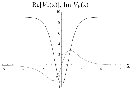
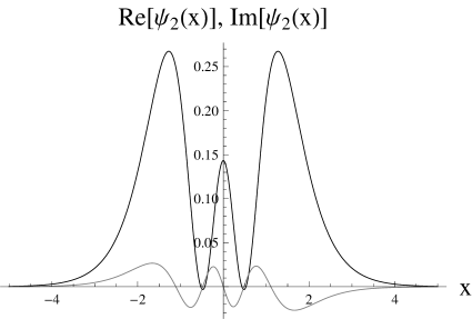
Figure 1: Left plot: graph of the real part (black curve) and imaginary part (grey curve) of the potential (LABEL:pot1ptx) with $n=2$ and $k=0.1$. Right plot: graph of the real part (black curve) and imaginary part (grey curve) of (29) for $n=2$ and $k=0.01$.

Similar to the case of the Wronskian (LABEL:wron1), the exponential terms in (29) remain bounded, such that behaviour at the infinities is determined by the hyperbolic secant function that is taken to the eighth power. Since this function falls more rapidly than the remaining hyperbolic sine and cosine functions grow, the function (29) tends exponentially to zero at both positive and negative infinify. As a consequence, the integral in (11) exists. Now, since there are only three functions in (24) due to the constraint $n<3$, we can calculate their norm integrals numerically once a particular value for the parameter $a$ is chosen. We pick $k=0.1$, this gives

$$\begin{array}[]{llllllll}N(\Psi_{0})~{}=~{}1.06667&&N(\Psi_{1})~{}=~{}-1.66462&&N(\Psi_{2})~{}=~{}0.745127.\end{array}$$ (31)

We observe that our pseudo-norm alternates in sign. This is a known phenomenon to occur in the context of ${\cal PT}$-symmetry [19]. Since going into further details regarding alternating-sign pseudo-norms is beyond the scope of this work, we refer the reader to [8]. Now, using the results from (31), we are now able to normalize our solutions (24). The correctly normalized solutions are simply given by $\hat{\Psi}_{n}=\Psi_{n}/N(\Psi_{n})$, $0\leq n<3$.

Example: generalization of Yekken’s system.

In this paragraph we will show that our boundary-value problem (1), (2) with potential (17) generalizes a model studied by Yekken and collaborators [33]. In the latter reference, the following potential is considered

$$V_{E}(x) = -\lambda~{}(1+\gamma~{}E_{n}^{\nu})~{}\mbox{sech}^{2}(x),$$ (32)

where $\lambda$, $\nu$ and $\gamma$ are real-valued constants. In order to recover a generalization of (32), we apply the following settings to our potential (17)

$$A~{}=~{}-\frac{\alpha}{2}+\frac{1}{2}~{}\sqrt{\alpha^{2}+4~{}\lambda}\qquad\qquad B(E)~{}=~{}i~{}\exp\left(\frac{\nu}{2}\right)~{}\sqrt{\gamma~{}\lambda}.$$ (33)

Upon substitution of these parameters, the potential (17) takes the form

$$V_{E}(x) = \frac{1}{4}\left(-\alpha+\sqrt{\alpha^{2}+4~{}\lambda}\right)-\lambda~{}\left(1+\gamma~{}E_{n}^{\nu}\right)\mbox{sech}^{2}\left(\alpha x\right)+$$ (34)

$$+ i~{}E_{n}^{\frac{\nu}{2}}\sqrt{\gamma~{}\lambda~{}(\alpha^{2}+4~{}\lambda)}~{}\mbox{sech}(\alpha x)~{}\tanh(\alpha x),$$

recall that the energies $E_{n}$ are given in (18). Since for $\alpha=1$ the second term on the right side coincides with its counterpart in (32), we have constructed a complex, energy-dependent generalization of the latter potential. The discrete energies and associated solutions to the boundary-value problem with potential (34) can be obtained by plugging the settings (33) into (18) and (19), respectively. For the sake of brevity we omit to state the resulting expressions.

4.2 Trigonometric Scarf system

The next application we present is governed by the boundary-value problem (1), (2), defined on the bounded domain $D=(-\pi/(2\alpha),\pi/(2\alpha))$ for a constant $\alpha>0$ and endowed with the potential

$$V_{E}(x) = -A^{2}+\left[B(E)^{2}+A^{2}-A~{}\alpha\right]\mbox{sec}^{2}(\alpha x)-B(E)~{}(2A-\alpha)~{}\tan(\alpha x)~{}\mbox{sec}(\alpha x),$$ (35)

where the constants $A$, $\alpha$ are positive and $B$ is a complex-valued function of the energy $E$. We observe that (35) generalizes the trigonometric Scarf potential, featuring energy-dependence and complex values. It should be mentioned that (35) can be generated from its hyperbolic counterpart (17) by making the simultaneous replacements $A\rightarrow-A$, $B\rightarrow B^{\ast}$, $x\rightarrow ix$ and flipping the overall sign of the potential. Since the discrete energies (18) in the hyperbolic case do not depend on the parameter $B$, the aforementioned link between the hyperbolic and the trigonometric case implies that our potential (35) is associated with real discrete energies and that it becomes ${\cal PT}$-symmetric if the real part of $B$ vanishes. Solutions of our boundary-value problem (1), (2) for the potential (35) can be constructed provided the energy takes discrete values $E=E_{n}$, where $n$ is a nonnegative integer. These energy values are given by

$$E_{n} = -A^{2}+(A+\alpha~{}n)^{2},~{}~{}~{}n=0,1,2,...$$ (36)

As in the previous two applications, these discrete energies are real-valued. Now, the solutions of our problem associated with (36) are given by

$$\Psi_{n}(x)=\left[1-\sin\left(\alpha x\right)\right]^{\frac{A-B(E_{n})}{2\alpha}}\left[1+\sin\left(\alpha x\right)\right]^{\frac{A+B(E_{n})}{2\alpha}}P_{n}^{\left(-\frac{1}{2}+\frac{A}{\alpha}-\frac{B(E_{n})}{\alpha},-\frac{1}{2}+\frac{A}{\alpha}+\frac{B(E_{n})}{\alpha}\right)}\left[\sin\left(\alpha x\right)\right].$$ (37)

As before, $P_{n}$ denotes the Jacobi polynomial of degree $n$. In order to check that our boundary conditions (2) are fulfilled at $\pm~{}\pi/(2\alpha)$, we inspect the first two factors on the right side of (37). These factors vanish at $-\pi/(2\alpha)$ and $\pi/(2\alpha)$, respectively, provided the real part of their exponents remains positive. This is true as long as the constraint

$$|\mbox{Re}[B(E_{n})]| < A,$$ (38)

is satisfied. This constraint leads to an interesting situation concerning the number of solutions (37) to our boundary-value problem. Since $E_{n}$ changes with $n$, so do $B(E_{n})$ and the functions (37). It is therefore possible that for certain values of $n$ the constraint (38) is not fulfilled, such that the associated solutions from (52) do not satisfy the boundary conditions. As an illustration let us now assume that $A=5,\alpha=1$ and Re$[B(E_{n})]=1/10$. The constraint (38) then takes the form

$$\frac{n~{}(n+10)}{10} < 5.$$

Solving for $n$ gives the result

$$n~{}<~{}-5+5~{}\sqrt{3}~{}\approx~{}3.66025.$$ (39)

Since $n$ takes only integer values, the latter identity amounts to $n\leq 3$. Consequently, our boundary-value problem (1), (2) for the trigonometric Scarf potential (41) has four solutions (43), corresponding to the parameter values $n=0,...,3$. Since in this example the real part of $B$ does not vanish, the underlying system is not ${\cal PT}$-symmetric.

Example.

Let us now choose the parameters in our potential (35) as follows

$$A~{}=~{}5\qquad\qquad\qquad\alpha~{}=~{}1\qquad\qquad\qquad B(E)~{}=~{}b~{}\sqrt{E+1},$$ (40)

where $b>0$ is a constant. Our choices for the parameter values of $A$ and $\alpha$ follow the same reason as (20) in the previous example. Similarly, $B$ was chosen to have a simple energy-dependence. Note that we must add one inside the radicand, as otherwise the lowest bound state solution for $n=0$ will be undefined. Since the parameter $B$ is purely imaginary, the system governed by the potential (35) is ${\cal PT}$-symmetric. In addition, the limiting condition (38) is always satisfied. Upon substitution of our settings (40), the latter potential takes the form

$$V_{E}(x)=-25+\Bigg{\{}20-b^{2}\Bigg{[}1+n~{}(n+10)\Bigg{]}\Bigg{\}}\sec^{2}(x)-9~{}i~{}b~{}\sqrt{1+n~{}(n+10)}\Bigg{]}\sec(x)\tan(x).$$

(41)

A particular case of this potential is shown in the left plot of figure 2. Our boundary-value problem (1), (2) for the potential (41) admits solutions if the energy takes the discrete values obtained from (36) after substitution of our settings (40)

$$E_{n} = n~{}(n+10),~{}~{}~{}n=0,1,2,....$$ (42)

The solutions associated with these energies can be constructed by means of plugging (40) into (37). This yields

$$\Psi_{n}(x) = \left[1-\sin\left(x\right)\right]^{\frac{5}{2}-\frac{ib\sqrt{n~{}(n+10)+1}}{2}}\left[1+\sin\left(x\right)\right]^{\frac{5}{2}+\frac{ib\sqrt{n~{}(n+10)+1}}{2}}\times$$ (43)

$$\times P_{n}^{\left(\frac{9}{2}-ib\sqrt{n(n+10)+1},\frac{9}{2}+ib\sqrt{n(n+10)+1}\right)}\left[\sin\left(x\right)\right],$$

where $n=0,1,2,...$. Next, let us establish orthogonality of our solutions using the Wronskian representation (15). We get for admissible integers $m,n$ with $m\neq n$

$$W_{{\cal PT}\Psi_{m},\Psi_{n}}(x) = \frac{1}{2}\left[\frac{1-\sin\left(x\right)}{1+\sin\left(x\right)}\right]^{-\frac{1}{2}ib\left[\sqrt{m(m+10)+1}+\sqrt{n(n+10)+1}\right]}~{}\cos^{9}(x)~{}\times$$ (44)

$$\times~{}~{}\Bigg{\{}(m+10)~{}\cos^{2}(x)~{}P^{\ast}_{m-1}(-x)~{}P_{n}(x)+2~{}P^{\ast}_{m}(-x)~{}P_{n}(x)\Bigg{[}(n+1))~{}\cos^{2}(x)~{}P_{n-1}(x)-$$

$$-~{}2~{}i~{}b~{}\left[\sqrt{m(m+10)+1}+\sqrt{n(n+10)+1}\right]P_{n}(x)\Bigg{]}\Bigg{\}},$$

where the following abbreviation is in use

$$P_{j-k}(x)=\left\{\begin{array}[]{lll}P_{j-k}^{\left(k+\frac{9}{2}-ib\sqrt{j(j+10)+1},k+\frac{9}{2}+ib\sqrt{j(j+10)+1}\right)}\left[\sin\left(x\right)\right]&\mbox{if}&j-k\geq 0\\[4.30554pt] 0&\mbox{if}&j-k<0\end{array}\right\}.$$ (47)

Note that $j,k$ are nonnegative integers. It is straightforward to verify that the first two terms on the right side of (44) guarantee vanishing of the Wronskian at $\pm\pi/2$ in both real and imaginary part. As an immediate consequence the left side of (16) equals zero upon identifying $a=-\pi/2$ and $b=\pi/2$. This implies that the functions in (43) are orthogonal with respect to (3.1). Now, the remaining task is to evaluate the pseudo-norm (12) for our solutions. After substituting (41), (43) and (42), the integrand on the right side of (12) takes the following form

$$\Psi^{\ast}_{n}(-x)~{}\Psi_{n}(x)\left[1-\frac{\partial V_{E}(x)}{\partial E}\right]_{\big{|}E=E_{n}} =$$ (49)

$$=~{}\left[1-\sin\left(x\right)\right]^{5-ib\sqrt{n(n+10)+1}}\left[1+\sin\left(x\right)\right]^{5+ib\sqrt{n(n+10)+1}}\times$$

$$\times~{}P^{\ast}_{n}(-x)~{}P_{n}(x)\Bigg{[}1+b^{2}~{}\sec^{2}(x)+\frac{9~{}i~{}b}{2~{}\sqrt{n~{}(n+10)+1}}~{}\sec(x)~{}\tan(x)\Bigg{]}.$$

Observe that we have used the abbreviation (LABEL:abb3). The function (49) is displayed in the right plot of figure 2 for a particular parameter setting.

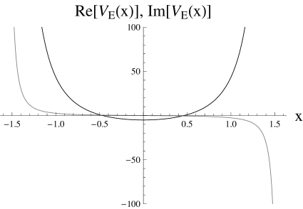
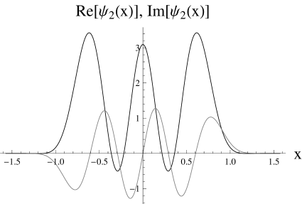
Figure 2: Left plot: graph of the real part (black curve) and imaginary part (grey curve) of the potential (41) with $n=0$, $b=0.1$. Right plot: graph of the real part (black curve) and imaginary part (grey curve) of (49) for $n=2$, $b=0.01$.

Similar to the case of (44), we can show that both real and imaginary part of the first two terms on the right side of (49) vanish at $\pi/2$ and $-\pi/2$, respectively. Continuity of (49) then implies existence of the pseudo-norm integral in (11). Since the constraint (38) is satisfied, there is no restriction on the number of bound-state solutions conatined in (43). Let us now determine their first four pseudo-norm integrals (12) numerically after assigning a specific value to our parameter $b$. Upon setting $b=0.01$, we obtain

$$N(\Psi_{0}) = 0.773111$$

$$N(\Psi_{1}) = -1.94853$$

$$N(\Psi_{2}) = 3.20699$$

$$N(\Psi_{3}) = -4.38392.$$

As in section 4.1, the pseudo-norm is alternating in sign [8] [19]. Upon using the above values, the correctly normalized solutions in (43) are obtained as $\Psi_{n}/N(\Psi_{n})$, $n=0,1,2,...$.

5 Energy-dependent Morse-type system

In our next application our boundary-value problem is defined on the domain $D=(-\infty,\infty)$ and equipped with the following potential

$$V_{E}(x) = A^{2}+B(E)^{2}~{}\exp\left(-2~{}\alpha~{}x\right)-2~{}B(E)~{}\left(A+\frac{\alpha}{2}\right)~{}\exp\left(-\alpha~{}x\right),$$ (50)

introducing positive constants $A$ and $\alpha$ are positive, while $B$ is a complex-valued function of the energy $E$. The function (50) is readily recognized as a complex, energy-dependent version of the Morse potential [11]. In contrast to the previous application, the present potential (50) does not feature ${\cal PT}$-symmetry unless we make the trivial assignment $B=0$. Despite this fact, we can show that (50) is pseudo-hermitian. To this end, we will use a result obtained in [4]. In the latter reference it was shown that pseudo-hermiticity is established by an operator $\eta$ of the form $\eta=\exp(-\theta~{}p)$, where $p=-i~{}d/dx$ and $\theta$ is a real constant that we will determine below for the present system. Using the latter operator $\eta$, the relation $\eta V_{E}\eta^{-1}=V^{\ast}_{E}$ is equivalent to

$$V_{E}(x+i~{}\theta) = V_{E}^{\ast}(x),$$

implying that the Hamiltonian associated with the system is $\eta$-pseudo-hermitian with respect to $\eta=\exp(-\theta p)$ (for the sake of brevity we will refer to our system simply as pseudo-hermitian). Including energy-dependence in the parameter $B$ allows to maintain pseudo-hermiticity, as we will demonstrate now. To this end, let us define a real-valued quantity $\theta$ by means of

$$\theta = \frac{2}{\alpha}~{}\arctan\left\{\frac{\mbox{Im}[B(E)]}{\mbox{Re}[B(E)]}\right\}.$$

We can express $\theta$ through complex logarithms as follows

$$\theta = \frac{i}{\alpha}~{}\log\left\{1-i~{}\frac{\mbox{Im}[B(E)]}{\mbox{Re}[B(E)]}\right\}-\frac{i}{\alpha}~{}\log\left\{1+i~{}\frac{\mbox{Im}[B(E)]}{\mbox{Re}[B(E)]}\right\}.$$

We will now use this $\theta$ to verify pseudo-hermiticity of our potential (50). First, we note that

$$\exp\left[-\alpha~{}(x+i~{}\theta)\right] = \exp(-\alpha~{}x)~{}\exp(-i~{}\alpha~{}\theta)$$

$$= \exp(-\alpha~{}x)~{}\left\{1-i~{}\frac{\mbox{Im}[B(E)]}{\mbox{Re}[B(E)]}\right\}\left\{1+i~{}\frac{\mbox{Im}[B(E)]}{\mbox{Re}[B(E)]}\right\}^{-1}$$

$$= \exp(-\alpha~{}x)~{}\frac{B(E)^{\ast}}{B(E)}.$$

Upon plugging this identity into our potential (50), we obtain

$$V_{E}(x+i~{}\theta) = A^{2}+\left[B(E)^{\ast}\right]^{2}\exp\left(-2~{}\alpha~{}x\right)-2~{}B(E)^{\ast}\left(A+\frac{\alpha}{2}\right)~{}\exp\left(-\alpha~{}x\right)~{}=~{}V_{E}^{\ast}(x).$$

This relation establishes pseudo-hermiticity of (50). Now, solutions to our boundary-value problem (1), (2) for the potential (50) exist if the energy takes the following discrete values $E=E_{n}$, where

$$E_{n} = A^{2}-\left(A-\alpha~{}n\right)^{2},$$ (51)

introducing a nonnegative integer $n$ satisfying $0\leq n<A/\alpha$. As in the previously discussed case of the hyperbolic Scarf potential, we see that the energies (51) are real despite the potential (50) taking complex values. The solutions $\Psi=\Psi_{n}$, $0\leq n<A/\alpha$, of our equation (1) and associated with our energies (51) read

$$\Psi_{n}(x) = \exp\left[-A~{}x+\alpha~{}n~{}x-\frac{B(E_{n})}{\alpha}~{}\exp(-\alpha~{}x)\right]~{}L_{n}^{\frac{2A}{\alpha}-2n}\left[\frac{2B(E_{n})}{\alpha}~{}\exp\left(-\alpha~{}x\right)\right],$$ (52)

where $L_{n}$ stands for an associated Laguerre polynomial of degree $n$ [1]. In order to verify that the functions (52) satisfy the boundary conditions (2) at positive and negative infinity, let us inspect the first exponential factor on the right side of (52). Due to the constraint $n<A/\alpha$, the latter factor, together with the Laguerre polynomial, dominates at positive infinity, guaranteeing exponential decay to zero in both real and imaginary part of the solutions. Next, the behaviour of (52) at negative infinity is governed by the double exponential. While the imaginary part of $B$ produces an oscillatory function, its real part must be positive in order to ensure vanishing of the solutions at negative infinity. In summary, our boundary conditions (2) are fulfilled only if the real part of $B$ is positive. The remaining task is to evaluate orthogonality condition and pseudo-norm, which we will perform within the following example.

Example.

In order to evaluate the orthogonality condition and the pseudo-norm we now choose the parameters $A,\alpha$ and $B$ as follows

$$A~{}=~{}3\qquad\qquad\qquad\alpha~{}=~{}1\qquad\qquad\qquad B(E)~{}=~{}1+i~{}k~{}E,$$ (53)

where $k>0$ is a constant. Recall that the real part of $B$ is allowed to depend on $E$. However, we chose it as a constant in order to simplify and shorten subsequent calculations. Similar to (20) and (40), parameter values were assigned in (53) such as to facilitate subsequent calculations. We now substitute the settings (53) into our potential (50), rendering it in the form

$$V_{E}(x) = 9-7~{}\exp(-x)~{}\left\{1+i~{}k~{}\left[9-(3-n)^{2}\right]\right\}+\exp(-2~{}x)\times$$ (54)

$$\times \left\{1+i~{}k~{}\left[9-(3-n)^{2}\right]\right\}^{2}.$$

Observe that this potential is real-valued for the particular value $n=0$. A particular example of (54) is displayed in figure 3. Next, we obtain the discrete energies by plugging (53) into (51). This gives

$$E_{n} = -n~{}(n-6),~{}~{}~{}n=0,1,2.$$ (55)

The solutions (52) associated with the present settings (53) take the form

$$\Psi_{n}(x) = \exp\Big{\{}-\exp(-x)\left[1+i~{}k~{}(6n-n^{2})\right]+(n-3)~{}x\Big{\}}\times$$ (56)

$$\times L_{n}^{-2n+6}\left\{2~{}\exp(-x)\left[1+i~{}k~{}(6n-n^{2})\right]\right\},$$

where $n=0,1,2$. Observe that the functions in (56) satisfy our boundary conditions (2) at the infinities because the real part of $B$ is positive, see (53). Our next task is to study orthogonality of the functions (56). As in the previous case of the hyperbolic Scarf potential, we will use a Wronskian representation, but this time we need the version (15). For admissible integers $m,n$ satisfying $m\neq n$ we find the Wronskian of $\Psi^{\ast}_{m}$ and $\eta\Psi_{n}$ as

$$W_{\Psi^{\ast}_{m},\eta\Psi_{n}}(x) = \exp\Bigg{\{}\exp(-x)\Big{\{}-2-i~{}k~{}\Big{[}m~{}(m-6)+n~{}(n-6)\Big{]}+$$ (57)

$$+~{}\exp(x)~{}x~{}(m+n-7)-2~{}i~{}\exp(x)~{}(n-3)~{}\arctan\Big{[}k~{}n~{}(n-6)\Big{]}\Big{\}}\Bigg{\}}~{}\times$$

$$\times~{}\Bigg{\{}-2~{}\Big{[}1+i~{}k~{}m~{}(m-6)\Big{]}L^{\ast}_{m-1}(x)~{}\hat{L}_{n}(x)+\Big{[}1+\exp(x)~{}(m-3)+$$

$$+~{}i~{}k~{}m~{}(m-6)\Big{]}~{}L^{\ast}_{m}(x)~{}\hat{L}_{n}(x)+L^{\ast}_{m}(x)\Bigg{[}2~{}\Big{\{}2~{}\exp\Big{[}2~{}i~{}\arctan[k~{}n~{}(n-6)]\Big{]}\times$$

$$\times~{}\Big{[}1-i~{}k~{}n~{}(n-6)\Big{]}~{}L_{n-1}(x)+\Big{\{}\exp(x)~{}(n-3)+\exp\Big{[}2~{}i~{}\arctan[k~{}n~{}(n-6)]\Big{]}\times$$

$$\times~{}\Big{[}1-i~{}k~{}n~{}(n-6)\Big{]}[1-i~{}k~{}n~{}(n-6)]~{}\hat{L}_{n}(x)\Big{\}}\Bigg{]}\Bigg{\}}.$$

For the sake of brevity we used the following abbreviations for the associated Laguerre polynomials that appear in the latter Wronskian

$$L_{j-l}(x) = \left\{\begin{array}[]{llllll}L_{j-l}^{l-2j+6}\left\{2\exp(-x)\left[1-i~{}k~{}(6j-j^{2})\right]\right\}&\mbox{if}&j-l\geq 0\\[4.30554pt] 0&\mbox{if}&j-l<0\end{array}\right\}$$ (60)

$$\hat{L}_{j-l}(x) = \left\{\begin{array}[]{llllll}L_{j-l}^{l-2j+6}\left\{2\exp\Big{[}2~{}i~{}\arctan[k~{}n~{}(n-6)]\Big{]}\left[1-i~{}k~{}(6j-j^{2})\right]\right\}&\mbox{if}&j-l\geq 0\\[4.30554pt] 0&\mbox{if}&j-l<0\end{array}\right\},$$ (63)

where $j,l=0,1,2$. In order to show that the functions in (56) satisfy the orthogonality relation (15), we study the behaviour of the Wronskian (57) at the infinities. First we observe that both the first exponential factor on the right side of (57) as well as the Laguerre polynomials tend to zero in real and imaginary part as $x$ goes to positive infinity. As a consequence, the Wronskian vanishes there. The behaviour of our Wronskian at negative infinity is governed by terms located in the first exponential factor on the right side of (57). More precisely, the terms dominant at negative infinity read

$$W_{\Psi^{\ast}_{m},\eta\Psi_{n}}(x) \stackrel{{\scriptstyle x<<-1}}{{\sim}}\exp\Bigg{\{}-\exp(-x)~{}\Big{\{}2+i~{}k~{}\Big{[}m~{}(m-6)+n~{}(n-6)\Big{]}\Big{\}}\Bigg{\}}.$$ (65)

This term vanishes at negative infinity in both real and imaginary part. Even though the Laguerre polynomials in (57) grow exponentially as $x$ tends to negative infinity, they cannot compensate the double exponential decay from (65). Consequently, the Wronskian (57) vanishes at both infinities. According to (15), this implies orthogonality of the functions in (56). The final task is now to prove normalizability of the latter functions. Since there are only three of such functions due to $n<3$, we proceed in a way that is similar to the previous application. In the first step we establish existence of the integral in (11). To this end, we evaluate

$$\Psi^{\ast}_{n}(x)~{}\eta~{}\Psi_{n}(x)\left[1-\frac{\partial V^{\ast}_{E}(x)}{\partial E}\right]_{\big{|}E=E_{n}} =$$ (66)

$$=~{}\exp\Bigg{\{}-\exp(-x)~{}\Big{\{}-2-2~{}i~{}k~{}n~{}(n-6)+2~{}\exp(x)~{}x~{}(n-4)-$$

$$-~{}2~{}i~{}\exp(x)~{}(n-3)~{}\arctan[k~{}n~{}(n-6)]\Big{\}}\Bigg{\}}\Bigg{\{}\exp(2~{}x)-7~{}i~{}k~{}\exp(x)+$$

$$+~{}2~{}k~{}[i-k~{}n~{}(n-6)]\Bigg{\}}~{}L^{\ast}_{n}(x)~{}\hat{L}_{n}(x).$$

Note that here we have used once more the abbreviations (LABEL:abbl) for the associated Laguerre polynomials. The right plot in figure 3 shows an example of (66).

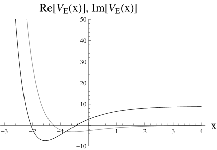
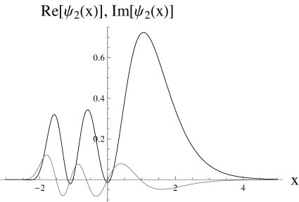
Figure 3: Left plot: graph of the real part (black curve) and imaginary part (grey curve) of the potential (50) with $n=1$ and $k=0.1$. Right plot: graph of the real part (black curve) and imaginary part (grey curve) of (66) for $n=2$ and $k=0.01$.

It turns out that the function (66) vanishes at the infinities. The reasoning is very similar to the argumentation that we presented above for the case of our Wronskian (57), such that we omit to show it here. It follows that the integral in (11) exists in the present case, such that we can proceed to calculate its value numerically. We find for the three applicable cases

$$N(\Psi_{0}) = 1.875$$

$$N(\Psi_{1}) = 1.86566$$

$$N(\Psi_{2}) = 1.49046.$$ (67)

The correctly normalized solutions (56) are now obtained from (67) by means of $\Psi_{n}/N(\Psi_{n})$, $n=0,1,2$.

6 Concluding remarks

In this work we have studied examples of quantum systems featuring complex-valued, energy-dependent potentials that admit real energy spectra and normalizable solutions forming orthogonal sets. While bound-state solutions belonging to pseudo-hermitian or ${\cal PT}$-symmetric systems are usually normalized in a weighted $L^{2}$-space, in the present cases we have normalized using the definition (11), which stems from the modified quantum theory applicable to systems with energy-dependent potentials. Investigation of the relationship between both types of normalization is subject to future research. Before we conclude this work, let us comment on the applicability of the results that we have obtained. One of the principal application fields of complex potentials featuring energy-dependence is nuclear physics [6] [23] [24], particularly the calculation of expectation values and bound-state normalization constants. Since for energy-dependent potentials one has to adhoc-modify the inner product and norm of the former underlying Hilbert space, there are several possibilities of doing so. Besides the conventional approach [16] [17] [24], for pseudo-hermitian or ${\cal PT}$-symmetric potentials our work suggests alternative ways of calculating expectation values and determining normalization constants through our modified norms (11) and (12), respectively. In practical applications such as [24], results given by our norms may be compared with existing results and experimentally obtained findings.

References

- [1] M. Abramowitz and I. Stegun, Handbook of Mathematical Functions with Formulas, Graphs, and Mathematical Tables, (Dover Publications, New York, 1964)
- [2] Z. Ahmed and J.A. Nathan, Real discrete spectrum in the complex non--symmetric Scarf II potential, Phys. Lett. A 379 (2015), 865-869
- [3] Z. Ahmed, Real and complex discrete eigenvalues in an exactly solvable one-dimensional complex PT -invariant potential”, Phys. Lett. A 282 (2001), 343
- [4] Z. Ahmed, Pseudo-hermiticity of Hamiltonians under imaginary shift of the coordinate: real spectrum of complex potentials, Phys. Lett. A 290 (2001), 19-22
- [5] Z. Ahmed, Real and complex discrete eigenvalues in an exactly solvable one-dimensional complex -invariant potential, Phys. Lett. A 282 (2001), 343-348
- [6] G. Alberi and G. Ghirardi, Energy dependent complex potentials and bound states, Nucl. Phys. 87 (2016), 470-476
- [7] C.M. Bender, Making sense of non-hermitian Hamiltonians, Rept. Prog. Phys. 70 (2007), 947-1018
- [8] C.M. Bender, Introduction to -symmetric Quantum Theory, Contemp. Phys. 46 (2005), 277-292
- [9] C.M. Bender and S. Boettcher, Real Spectra in Non-Hermitian Hamiltonians Having PT Symmetry, Phys. Rev. Lett. 80, 5243-5246 (1998)
- [10] A. Contreras-Astorga and A. Schulze-Halberg, On integral and differential representations of Jordan chains and the confluent supersymmetry algorithm, J. Phys. A 48 (2015), 315202
- [11] J. Derezinski and M. Wrochna, Exactly solvable Schrödinger operators, Annales Henri Poincare 12 (2011), 397-418
- [12] J. Formanek, R.J. Lombard and J. Mares, Wave equations with energy-dependent potentials, Czech. J. Phys. 54 (2004), 289
- [13] J. Garcia-Martinez, J. Garcia-Ravelo, J.J. Pena and A. Schulze-Halberg, Exactly solvable energy-dependent potentials, Phys. Lett. A 373 (2009), 3619-3623
- [14] U. Günther, B.F. Samsonov and F. Stefani, A globally diagonalizable -2-dynamo operator, SUSY QM, and the Dirac equation, J. Phys. A 40 (2007), F169-F176
- [15] Y. Li, Some water wave equations and integrability, J. Nonlin. Math. Phys. 12 (2005), 466-481
- [16] N. Hokkyo, A remark on the norm of the unstable state, Progr. Theoret. Phys. 33 (1965), 1116-1128
- [17] N. Hokkyo, Erratum, Progr. Theoret. Phys. 34 (1965), 328
- [18] P.A. Kalozoumis, C.V. Morfonios, F.K. Diakonos, and P. Schmelcher, -symmetry breaking in waveguides with competing loss-gain, Phys. Rev. A 93 (2016), 063831
- [19] G. Levai, F. Cannata and A. Ventura, PT-symmetry breaking and explicit expressions for the pseudo-norm in the Scarf II potential, Phys. Lett. A 300 (2002), 271-281
- [20] R.J. Lombard, J. Mares and C. Volpe, Wave equation with energy-dependent potentials for confined systems, J. Phys. G 34 (2007), 1-11
- [21] M. Maamache, Periodic pseudo-Hermitian Hamiltonian: Nonadiabatic geometric phase, Phys. Rev. A 92 (2015), 032106
- [22] B.P. Mandal and S. Gupta, Pseudo-hermitian interaction in relativistic quantum mechanics, Mod. Phys. Lett. A 25 (2010) 1723
- [23] B.H.J. McKellar and C.M. McKay, Formal scattering theory for energy-dependent potentials, Aus. J. Phys. 36 (1983), 607-616
- [24] K. Miyahara and T. Hyodo, Structure of and construction of local potential based on chiral dynamics, Phys. Rev. C 93 (2016), 015201
- [25] V. Milanovic and Z. Ikonic, On the optimization of resonant intersubband nonlinear optical susceptibilities in semiconductor quantum wells, IEEE J. Quantum Electron. 32 (1996), 1316-1323
- [26] J. Mourad and H. Sazdjian, The two-fermion relativistic wave equations of constraint theory in the Pauli-Schrödinger form, J. Math. Phys. 35 (1994), 6379-6406
- [27] A. Mostafazadeh, Pseudo-hermitian representation of quantum mechanics, Int. J. Geom. Meth. Mod. Phys. 7 (2010), 1191-1306
- [28] O. Panella and P. Roy, Pseudo Hermitian interactions in the Dirac Equation, Symmetry 6 (2014), 103-110
- [29] C.E. Rüter, K.G. Makris, R. El-Ganainy, D.N. Christodoulides, M. Segev, and D. Kip, Observation of parity-time symmetry in optics, Nature Physics 6 (2010), 192 - 195
- [30] J. Schindler, A. Li, M.C. Zheng, F.M. Ellis, and T. Kottos, Experimental study of active LRC circuits with -symmetries, Phys. Rev. A 84 (2011), 040101
- [31] L.S. Simeonov and N.V. Vitanov, Dynamical invariants for pseudo-hermitian Hamiltonians, Phys. Rev. A 93 (2016), 012123
- [32] S. C. L. Srivastava and S.R. Jain, Pseudo-Hermitian random matrix theory, Fortschr. Phys. 61 (2013), 276
- [33] R. Yekken, M. Lassaut and R.J. Lombard, Bound States of Energy Dependent Singular Potentials, Few-Body Syst 54 (2013), 2113 2124
- [34] R. Yekken, M. Lassaut and R.J. Lombard, Applying supersymmetry to energy dependent potentials, Ann. Phys. 338 (2013), 195-206
- [35] A.A. Zyablovsky, A.P. Vinogradov, A.A. Pukhov, A.V. Dorofeenko, and A A Lisyansky, -symmetry in optics, Physics - Uspekhi 57 (2014), 1063-1082