070018 2015 R. Dickman M. Hutter, Australian National University, Canberra, Australia. 070018

In this paper, a Bayesian method for piecewise regression is adapted to handle counting processes data distributed as Poisson. A numerical code in Mathematica is developed and tested analyzing simulated data. The resulting method is valuable for detecting breaking points in the count rate of time series for Poisson processes.

Bayesian regression of piecewise homogeneous Poisson processes

99 inst1 Departamento de Física y Química, Escuela de Formación Básica. Facultad de Ciencias Exactas, Ingeniería y Agrimensura. Universidad Nacional de Rosario, Av. Pellegrini 250, S2000BTP Rosario, Argentina.

1 Introduction

Bayesian statistics have revolutionized data analysis [1]. Techniques like the Generalized Lomb-Scargle Periodogram [2] allow us to obtain oscillation frequencies of time series with unprecedented accuracy. The Gregory and Loredo method [3] goes further allowing us to find and characterize periodic signals of any period and shape.

To detect non-periodical variations, the Exact Bayesian Regression of Piecewise Constant Functions by Marcus Hutter (hereafter Hutter’s method) [4] is valuable. It permits to estimate the most probable partition of a data set in segments of constant signals, determining the number of segments and their borders, and in-segments means and variances. Hutter’s method works with two continuous distributions: Normal, and Cauchy-Lorentz. The latter —the canonical example of a pathological distribution with undefined moments—, is also suitable to analyze data with other symmetric probability distributions, especially with heavy tails.

In the case of counting processes, especially for low rates, when data consist in non-negative small integers, methods specially designed to discrete probability distributions are necessary. Some regression methods, specially for non-homogeneous Poisson processes [5], were developed.

In this paper, Hutter’s method is adapted for analyzing data distributed as Poisson. The results are summarized in a code in Mathematica [6]. It can be used to analyze data of several physical processes which follow the Poisson distribution (e.g., detection of photons in X-ray Astronomy, particles in nuclear disintegration, etc.), if sudden changes in detection rates are suspected.

2 Method

Hutter’s method is summarized in Table 1 of Ref. [4] in a pseudo C code which is divided in two blocks. The first one calculates moments $A^{k}_{ij}$ with $k=0,1,2$ of the PDF of the statistical models for segments of data $D_{ij}:=\{n_{i+1},\ldots,n_{j}\}$. The second one performs the regression from moments $A^{k}_{ij}$. The code developed in this work is divided in three blocks.

As the members of the Poisson distributions family are identified by one parameter -the mean rate $r$ of the Poisson process-, the PDF of the models for a segment $D_{ij}$ is [1]

$$P(r|D_{ij},I)=\frac{P(r|I)\,P(D_{ij}|r)}{P(D_{ij})},$$ (1)

where $P(r|I)$ is the prior of parameter $r$, $P(D_{ij}|r)$ is the likelihood of segment $D_{ij}$ for a given $r$, $P(D_{ij})$ is the global likelihood of the family, and $I$ represents a prior information.

Usually, the prior information consists of global quantities calculated from $D:=D_{0N}$, i.e., from all the data set. For Poisson processes, only one quantity is necessary: the mean rate $\hat{r}$. Considering the conjugate prior of the Poisson distribution [7], the prior results

$$P(r|\hat{r})=\frac{r^{\hat{r}-1}\,e^{-r}}{\Gamma(\hat{r})}.$$ (2)

For a Poisson process with rate $r$, the likelihood of a segment $D_{ij}$ is

$$P(D_{ij}|r)=\prod_{t=i+1}^{j}\frac{r^{n_{t}}\,e^{-r}}{n_{t}!}.$$ (3)

So, the moments of the posterior can be expressed in an analytical form

$$A^{k}_{ij}=\frac{\Gamma(k+\hat{r}+\sum_{t=i+1}^{j}n_{t})\,\prod_{t=i+1}^{j}\frac{1}{n_{t}!}}{\Gamma(\hat{r})\,(j-i+1)^{k+\hat{r}+\sum_{t=i+1}^{j}n_{t}}}.$$ (4)

Code block 1 calculates $A^{k}_{ij}$. It needs as input the time series to be analyzed (list data). The output are functions A0[i,j], A1[i,j] and A2[i,j] and integer n, which is the length of data.

Code block 1: Mathematica code to calculate $A^{k}_{ij}$.

⬇

n=Length[data];

r=Mean[data];

Do[

Do[

d=j-i; m=r+Sum[data[[t]],{t,i+1,j}];

A0[i,j]=(m-1)!/(Gamma[r]*(d+1)^m)*

Product[1/data[[t]]!,{t,i+1,j}];

A1[i,j]=m*A0[i,j]/(d+1);

A2[i,j]=(m+1)*A1[i,j]/(d+1);

,{j,i+1,n}];

,{i,0,n}];

As the second block of Hutter’s code only needs the moments $A^{k}_{ij}$ as inputs, it could work properly with no changes. It computes the evidence, the probability for $k$ segments and its MAP estimation $\hat{k}$, the probability of boundaries locations and the MAP locations of the $\hat{k}$ boundaries, the first and second in-segment moments, and an interesting regression curve that smooths the final result.

Nevertheless, for our specific problem, once the segments boundaries are obtained, we can estimate their means and variances straightforwardly, so we only use a part of Hutter’s second block, which is shown in code block 2. The logical of the algorithm is explained in Ref. [4]. Code block 2 needs as inputs A0[i,j], A1[i,j], A2[i,j] and n, all calculated in code block 1, and integer kmax, which is the maximum number of segments to be considered. The outputs are the evidence (e), the probability for $k$ segments (c[k]), its MAP (khat), the probability of boundaries locations (B[i]), and their MAP (that[p]).

Code block 2: Mathematica code to calculate breaking points.

⬇

Do[

L[0,i]=KroneckerDelta[i,0];

R[0,i]=KroneckerDelta[i,n];

,{i,0,n}];

Do[

Do[

L[k+1,i]=Sum[L[k,h]*A0[h,i],{h,k,i-1}];

R[k+1,i]=Sum[R[k,h]*A0[i,h],{h,i+1,n-k}];

,{i,0,n}]

,{k,0,kmax-1}];

e=1/kmax*Sum[L[k,n]/Binomial[n-1,k-1],{k,1,kmax}];

Do[

c[k]=L[k,n]/(Binomial[n-1,k-1]*kmax*e)

,{k,1,kmax}];

khat=1;

Do[If[c[khat]<c[k],khat=k];,{k,0,kmax}];

Do[B[i]=

Sum[L[p,i]*R[khat-p,i]/L[khat,n],{p,0,khat}];

,{i,0,n}];

Do[

that[p]=0;

dummy=L[p,0]*R[khat-p,0];

Do[

If[dummy<L[p,h]*R[khat-p,h],

that[p]=h;

dummy=L[p,h]*R[khat-p,h];

];

,{h,1,n}];

,{p,0,khat}];

Finally, we calculate the in-segments means and estimate their statistical errors. If one segment of $m$ elements has $n$ counts, its mean rate is $n/m$, and its variance is approximately $n/m^{2}$.

To determine the accuracy of the fit, it is also useful to estimate the uncertainties of the boundaries locations. A reasonable estimation of the uncertainties can be obtained from the second moments of the probability distributions of boundaries locations in the neighborhoods of the breaking points. If the probabilities of the boundaries locations are given by function $B(k)$, the uncertainties approximately result

$$\epsilon_{\hat{k}}=\sqrt{\frac{\sum_{k=\hat{k}-a+1}^{\hat{k}+a}B(k)\,(k-\hat{k})^{2}}{\sum_{k=\hat{k}-a+1}^{\hat{k}-a}B(k)}},$$ (5)

where $a$ is large enough to consider all the width of the peak corresponding to boundary $\hat{k}$, but small enough to avoid including peaks of other boundaries. In practice, if $\hat{\j}$, $\hat{k}$ and $\hat{l}$ are the positions of consecutive boundaries, a good value for $a$ is the minimum of $(\hat{k}-\hat{\j})/2$ and $(\hat{l}-\hat{k})/2$.

Code block 3 uses these approaches to calculate the constant piecewise regression of data, and to estimate its statistical errors. The inputs are c[k], khat, B[i] and that. The outputs are list reg, which represents the best fit, and lists re1 and re2, which represent the minimum and maximum estimations considering the statistical errors of reg.

Code block 3: Mathematica code to calculate regression.

⬇

TBP=DeleteDuplicates[Table[that[k],{k,0,khat}]];

NBP=Length[TBP]-1;

Do[BP[k]=TBP[[k+1]];,{k,0,NBP}];

ethat[0]=0;ethat[NBP]=0;

Do[

l1=IntegerPart[(BP[k-1]+BP[k])/2]+1;

l2=IntegerPart[(BP[k+1]+BP[k])/2];

ethat[k]=

Round[Sqrt[Sum[(j-BP[k])^2*B[j],{j,l1,l2}]/

Sum[B[j],{j,l1,l2}]]];

,{k,1,NBP-1}];

Do[

mm[k]=BP[k]-BP[k-1];

nn[k]=Sum[data[[i]],{i,BP[k-1]+1,BP[k]}];

,{k,1,NBP}];

reg=Flatten[Table[Table[nn[k]/mm[k]

,{BP[k]-BP[k-1]}],{k,1,NBP}]];

BP1[0]=BP2[0]=BP[0];BP1[NBP]=BP2[NBP]=BP[NBP];

Do[

s=If[reg[[BP[k]+1]]>reg[[BP[k]]],1,-1];

BP1[k]=BP[k]+s*ethat[k];

BP2[k]=BP[k]-s*ethat[k];

,{k,1,NBP-1}];

re1=Flatten[Table[Table[(nn[k]-Sqrt[nn[k]])/mm[k]

,{BP1[k]-BP1[k-1]}],{k,1,NBP}]];

re2=Flatten[Table[Table[(nn[k]+Sqrt[nn[k]])/mm[k]

,{BP2[k]-BP2[k-1]}],{k,1,NBP}]];

3 Applications and Discussion

Figure 1 (top) shows, in blue dots, data simulated using Mathematica. Data consist of 150 Poisson distributed elements, the first 50 with rate $1.5$, the second 50 with rate $0.5$, and the last 50 with rate $1.0$. Applying the first 2 blocks of code on data, we can see that the probability of having 2 breaking points is very high. Figure 1 (top) also shows, in red line, the probability for the boundaries locations. Applying code block 3, we obtain the regression [Fig. 1 (bottom), black dashed curve] and its error estimation [Fig. 1 (bottom), gray zone]. The continuous blue line in Fig. 1 (bottom) indicates the rates used in simulation.

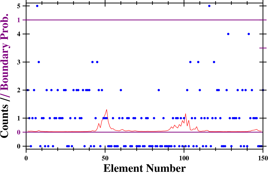
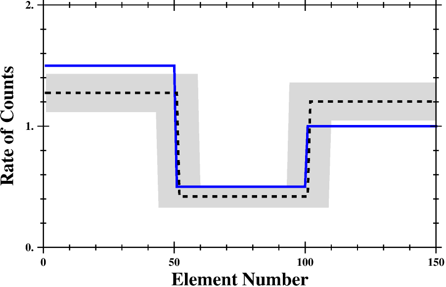
Figure 1: Top: Simulated data (blue dots) and boundaries location probability (red line). Bottom: Regression curve and its error estimation (black dashed line and gray zone), and the rate curve used in simulation (blue line).

The regression in the example above fits very well with the rate curve used in simulation. But sometimes regressions result qualitatively different to the rate curve, showing more or less breaking points, even for data simulated in the same conditions. This effect is due to chance. To show this issue, 2000 simulations with the same conditions were performed. In 992 of them, two breaking points were found. In the others, there were found zero (44), one (208), three (419), four (155), five (73), six (41), and seven or more (68) breaking points. For cases in which two breaking points were found, statistics of the most likely boundaries locations and in-segment mean rates were calculated. Figure 2 shows histograms of those statistics.

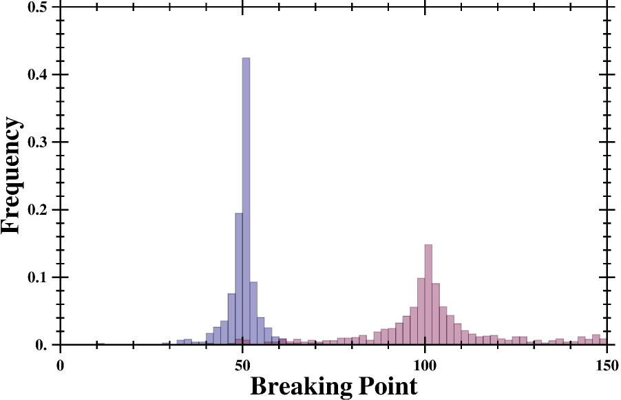
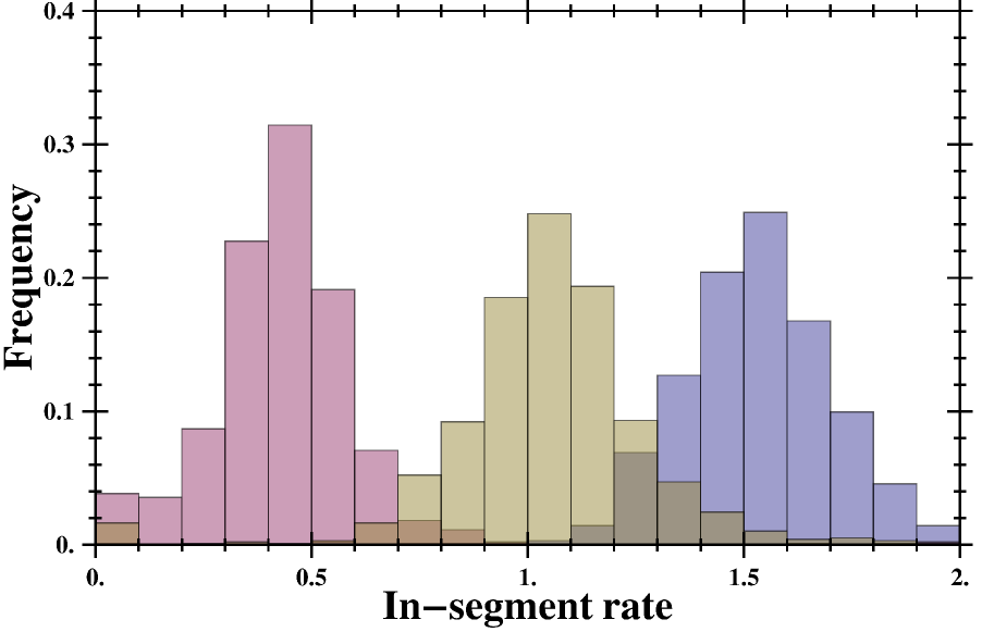
Figure 2: Top: Histogram of the boundaries locations. Bottom: Histogram of the in-segment mean rates. Both figures were calculated for a set of 2000 simulations similar to that shown in Fig. 1.

Figure 2 (top) shows histograms for boundaries locations. It is clear that the bigger the step, the smaller the uncertainty on its location. Figure 2 (bottom) shows histograms of in-segment rates. It is clear that the greater the rate, the smaller its relative statistical error.

Figure 3 shows data and boundaries location probabilities for a simulation similar to the previous ones, but now with rates 3.0, 1.0 and 2.0. Comparing Fig. 1 (top) and Fig. 3 (top), we can see that in the latter one the boundaries locations are found more accurately.

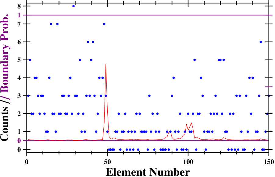
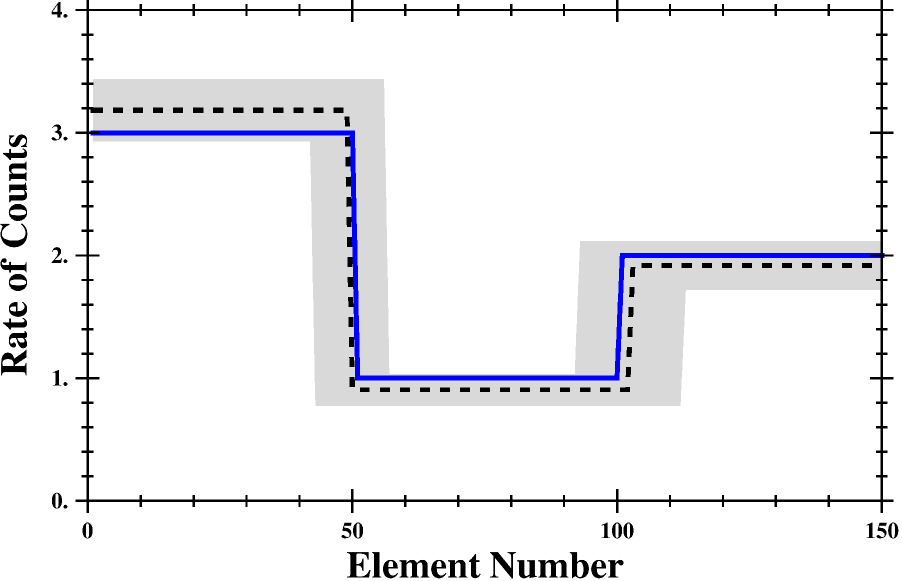
Figure 3: Top: Simulated data (blue dots) and boundaries location probability (red line). Bottom: Regression curve and its error estimation (black dashed line and gray zone), and the rate curve used in simulation (blue line).

Again, 2000 simulations with the same conditions were performed. In 1159 of them, two breaking points were found, while in the others, there were found zero (1), one (33), three (499), four (167), five (75), six (32), and seven or more (34) breaking points. Figure 4 shows histograms of the statistics of the most likely boundaries locations and in-segment rates for the simulations with two breaking points found. Comparing with Fig. 2, we can see that the histograms are now narrower. These results confirm what was stated above.

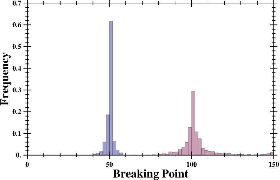
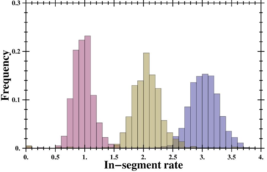
Figure 4: Top: Histogram of the boundaries locations. Bottom: Histogram of the in-segment rates. Both figures were calculated for a set of 2000 simulations similar to that shown in Fig. 3.

It is important to note that the probability for the real curve to be completely inside the region defined by the error estimations of the regression is significantly less than one. It is easy to see why: if the errors were independent and equal to the standard error, the probability of satisfying $n$ error conditions simultaneously would be $0.68^{n}$. But even the actual probability could be lower, since it is clear that the errors must be dependent. Nevertheless, the error estimations presented here are useful to get an idea of the accuracy of the regression.

Finally, the capability to detect a breaking point with this code was tested for different count rates. To do this, simulated data sets of a single step in the count rate were used. Data sets consist in 100 Poisson distributed elements, the first 50 for a rate $r_{1}$ and the last 50 for a rate $r_{2}$. 1000 simulations were done for each pair $(r_{1},r_{2})$. Statistics of successful detections are presented in Table 1. A successful detection is considered when only one breaking point between elements 40 and 60 is detected.

Table 1 shows that the smaller is the mean rate difference and the smaller are the mean rates, the more difficult is the detection of the step. This result is expected because in a Poisson distribution the variance is equal to the mean.

Table 1: Statistics of successful detections for a single step.

$r_{1}$\$\,r_{2}$	3.0	2.0	1.6	1.2	0.8
0.4	0.86	0.74	0.70	0.63	0.46
0.8	0.77	0.70	0.60	0.36
1.2	0.69	0.61	0.30
1.6	0.65	0.28
2.0	0.60

4 Conclusions

In this work, a code for Bayesian regression of piecewise constant functions was adapted to handle data from Poisson processes. For this purpose, equations for calculating the moments of the posteriors of segments of data were found through Bayes theorem, considering the conjugate prior of the Poisson distribution as prior. These results, as well as part of Hutter’s method, were used to calculate the most probable number of segments and their boundaries. Procedures for calculating in-segments mean rates and the uncertainties of mean rates and boundaries locations are also provided. The resulting method is summarized in a code in Mathematica.

The code was applied to simulated data. Firstly, two examples with tree segments were analyzed. The code performed well in both cases considering the dispersion of data, and the results improved in the case of higher mean rates and mean rates differences. This occurs because of the statistical dispersion of Poisson distributed data, which is greater than the mean rate if the mean rate is lower than one.

Finally, simulations of data of a single step were analyzed for different rates, and statistics of the regressions with only one breaking point are presented in a table. This table shows the effect of the rates and rate differences in the regression accuracy, and, together with the errors estimations provided by the code, can serve as an indicator of the reliability of the method.

Supplementary material including the source code for the algorithms can be found at the journal website [8].