Recurring OH Flares towards $o$ Ceti: I. location and structure of the 1990s’ and 2010s’ events

Abstract

We present the analysis of the onset of the new 2010s’ OH flaring event detected in the OH ground-state main line at 1665 MHz towards $o$ Ceti and compare its characteristics with those of the 1990s’ flaring event. This is based on a series of complementary single-dish and interferometric observations both in OH and H₂O obtained with the Nançay Radio telescope (NRT), the Medicina and Effelsberg Telescopes, the European VLBI Network (EVN), and (e)Multi-Element Radio Linked Interferometer Network ((e)MERLIN). We compare the overall characteristics of $o$ Ceti’s flaring events with those which have been observed towards other thin-shell Miras, and explore the implication of these events with respect to the standard OH circumstellar-envelope model. The role of binarity in the specific characteristics of $o$ Ceti’s flaring events is also investigated. The flaring regions are found to be less than $\sim$400$\pm$40 mas (i.e., $\leq 40\pm 4$ AU) either side of $o$ Ceti, with seemingly no preferential location with respect to the direction to the companion Mira B. Contrary to the usual expectation that the OH maser zone is located outside the H₂O maser zone, the coincidence of the H₂O and OH maser velocities suggests that both emissions arise at similar distances from the star. The OH flaring characteristics of Mira are similar to those observed in various Mira variables before, supporting the earlier results that the regions where the transient OH maser emission occurs are different from the standard OH maser zone.

1 Introduction

Asymptotic Giant Branch (AGB) stars have a high mass-loss rate (typically 10^-7 – 10^-5 M_⊙ yr^-1) leading to the creation of a dusty and molecular-rich circumstellar envelope (CSE). SiO, H₂O, and OH masers are commonly emitted by the CSEs of oxygen-rich AGB Miras and OH/IR stars. These masers are a powerful tool to study the dynamical and structural evolution of the CSE while the star evolves towards the [proto-]planetary nebula stage, which in turn is crucial in understanding e.g., how asymmetries, commonly observed in the proto-planetary nebula stage but not so much during the AGB evolution, develop.

In standard models, the CSE is in spherical radial expansion with masers tracing an ‘onion-shell’ structure (Omont 1988; Habing 1996). SiO is found closest to the star (typically within 4 R_∗, where R${}_{*}\sim$1 AU for a Mira), surrounded by H₂O (outside the radius where dust formation is complete) out to a few tens R_∗, whilst OH, created by the photodissociation of H₂O by external ambient UV radiation, is found in the outer part of the CSE (typically $\geq$100R_∗).

Miras are pulsating stars with periods ranging between $\sim$100 and $\sim$500 days. Long-term monitoring observations towards Miras revealed that the standard OH maser emission, though exhibiting slow modulation which spreads over several cycles, varies smoothly lagging behind the optical curve by about 10-20% of the period (Etoka & Le Squeren 2000). The polarisation of the overall emission, is typically $\leq$ 20% for the 1665/67-MHz main lines and $\leq$ 10% for the 1612-MHz satellite line (Wolak, Szymczak & Gérard, 2012).

Towards optically thin-shell Miras with low mass-loss rate, OH masers have shown particularly unexpected behaviour in the form of flares, that is the sudden emergence and subsequent fading away of strong OH maser emission in one of the ground-state lines, which can persist for several years. These flares occur at velocities close to the stellar velocity, suggesting that they emanate from closer to the star compared to the distance at which standard OH emission arises in the CSE (Jewell et al. 1981, Etoka & Le Squeren 1996, 1997), but this has never been confirmed by imaging.

$o$ Ceti, Mira ‘the wonderful’ has become synonymous with cool, pulsating AGB stars. With a distance estimated by HIPPARCOS to be 92 $\pm$11 pc (and a proper motion of PM${}_{\rm RA}=+9.33$ mas yr^-1 and PM${}_{\rm Dec}=-237.36$ mas yr^-1 van Leeuwen 2007), it is one of the closest Miras. It has an estimated mass-loss rate in the range of $\sim$[1 - 4] $\times$ 10^-7 ${\rm M_{\odot}yr^{-1}}$ (Knapp et al. 1998, Winters et al. 2003). Because of its typical optical period of 332 days, which has been monitored for centuries, it is also known as the prototype of Mira long-period variable stars. It actually belongs to a detached binary system (Mira AB) in which mass transfer by wind interaction is taking place. Sokolski & Bildsten (2010) found evidence pointing towards a white dwarf nature of Mira B, while $o$ Ceti (Mira A) shows clear signs of stellar asymmetry (Karovska et al. 1997; Reid & Menten 2007). $o$ Ceti and its companion Mira B are separated by only $\sim$0.5$\arcsec$ (Karovska et al. 1997), corresponding to $\sim$46 AU. The orbital elements of the system, originally determined by Baize (1980) lead to an orbital period of P$\sim$400 yr. A more recent revision by Prieur et al. (2002) leads to an increase of the estimation of the period by nearly 100 yr (the new estimated period being P$\sim$498 yr).

$o$ Ceti is associated with persistent SiO and H₂O masers (Cotton et al. 2006; Bowers & Johnston 1994). The first detection of OH maser emission in its CSE was made in 1974 (Dickinson, Kollberg & Yngvesson 1975) in the 1665-MHz ground-state main-line transition. The status of its OH ground-state maser lines at 1665, 1667 & 1612 MHz was checked with the NRT around an optical maximum phase in the late 1970’s down to a sensitivity limit of 70 mJy by Sivagnanam, Le Squeren & Foy (1988) who reported it as non-emissive.

Redetection of its OH-maser emission in the 1665-MHz line was made in November 1990 (Gérard & Bourgois 1993). The emission was then monitored at the NRT until it faded away nearly a decade later, late 2000. The strongest emission recorded in 2000 occurred on 23 November 2000 at phase $+0.21$ with a peak flux density of 250 mJy at a radial velocity of 46.7 km/s, which is believed to be the trail of the 1990s flare. Between December 2000 and December 2008, scattered observations of $o$ Ceti were made between phases $-0.42$ and $+0.45$ with 7 tentative detections at a level never exceeding 100 mJy. This does not exclude that the 1665-MHz level was ever present at a level $\leq$ 50 mJy. In November 2009 we detected with the NRT a new flare in the OH 1665-MHz line towards $o$ Ceti currently (2016) still active.

We present here a comparison of the 1990s’ flaring event characteristics with those of the 2010s’ event, based on a series of complementary single-dish and interferometric observations both in OH and H₂O with the Nançay, Medicina and Effelsberg Radio Telescopes, MERLIN and EVN-(e)MERLIN. The details of the observations are presented in section 2. The results of the OH and H₂O single-dish monitoring as well as the OH mappings obtained during the 1990s’ event and around the first OH maximum recorded during the new 2010s’ event are presented in section 3. A discussion of the results is given in section 4. Finally, a summary and conclusions are presented in section 5.

2 Observations and data reduction

2.1 The NRT OH observations

The NRT is a transit instrument with a half-power beamwidth of 3.5^′ in right ascension (RA) by 19^′ in declination (DEC) at 1.6 GHz.

For the 1990s’ observations, the system noise temperature was 45 K at ${\rm 0^{\circ}}$ declination. The antenna temperatures were converted to flux densities using the efficiency curve of the radiotelescope which was 0.9 ${\rm~{}K~{}Jy^{-1}}$ for point sources at ${\rm 0^{\circ}}$ declination. An autocorrelation spectrometer consisting of 4 banks of 256 channels was used to observe both left-hand and right-hand circular (LHC and RHC) polarisations of the two ground-state OH main lines at 1665 and 1667 MHz, providing Stokes parameters I and V. A bandwidth of 0.0975 MHz was used for each bank leading to a velocity resolution of 0.0703 km s^-1. Both linear vertical and horizontal polarisations (corresponding to the polarisation position angle PPA = $0^{\circ}$ and PPA = $90^{\circ}$, respectively) in the main lines were also regularly observed, providing the Stokes parameters I and Q. A typical observation, taken with a uneven sampling ranging from 1 day to $\sim$1.5 month, consisted in 40 minutes, taken in frequency switching mode, resulting in a mean rms of 100 mJy.

For the 2009/2010 observations presented here (corresponding to the time interval 2^d December 2009 – 21^th November 2010), the system temperature was about 35 K. The ratio of flux to antenna temperature was 1.4 ${\rm~{}K~{}Jy^{-1}}$ at ${\rm 0^{\circ}}$ declination. The 8192 channel autocorrelator was divided into 8 banks of 1024 channels each. A bandwidth of 0.195 MHz was used for each bank, leading to a velocity resolution of 0.0343 km s^-1. Prior and up to the first observation leading to the detection of the flare, observations were taken monthly over several years as part of a wider Key project. After the detection, the observations were taken every 5 days. Both ground-state main lines at 1665 MHz and 1667 MHz were recorded, and the ground-state satellite line at 1612 MHz was also regularly observed. A series of 2 successive observations of 30 minutes each in frequency switching mode were taken so as to obtain full polarimetric observations for both OH ground-state main lines in a similar fashion as described in Szymczak & Gérard (2004) hence providing the 4 Stokes parameters (I, Q, U and V) and the 2 circular (LHC, RHC) polarisations. This integration time provided a mean rms of about 90 mJy (decreasing to 55 mJy by “moving-average” smoothing over 3 channels when the signal was faint, hence degrading slightly the velocity resolution).

The flux-density scale accuracy for both epochs is $\sim$10%.

2.2 The interferometric OH observations

2.2.1 The MERLIN observations

The MERLIN 1665-MHz OH phase-referenced interferometric observations obtained during the 1990s’ flaring event were taken on the 28^th of November 1995 and the 4^th of May 1998. For the 1995 observations, the 8 telescopes of MERLIN available at that time (namely Defford, Cambridge, Knockin, Wardle, Darnhall, MK2, Lovell and Tabley) were used. The source was observed with a bandwith of 0.125 MHz divided into 128 channels at correlation, leading to a channel separation of 1 kHz (giving a velocity resolution of 0.18 km s^-1). For the 1998 observations, only six telescopes were used: Defford, Cambridge, Knockin, Darnhall, MK2 and Tabley. The source was observed with a bandwith of 0.25 MHz, divided into 256 channels at correlation, leading to the same channel separation as for the first epoch. For both epochs, J0219+0120, with a separation of 4.30^∘ from the target, was used as the phase-reference calibrator, 3C286 was used as the primary flux density reference, and the continuum source 3C84 was used to derive corrections for instrumental gain variations across the band. For both epochs the same pointing position was used for the source: RA${}_{\rm B1950}=02^{h}16^{m}49.062^{s}$ and DEC${}_{\rm B1950}=-03^{\circ}12\arcmin 22.480\arcsec$ (corresponding to RA${}_{\rm J2000}=02^{h}19^{m}20.771^{s}$ and DEC${}_{\rm J2000}=-02^{\circ}58\arcmin 36.674\arcsec$).

The initial editing, the gain-elevation correction and a first-order amplitude calibration of the MERLIN datasets were applied using the MERLIN-specific package DPROGRAMS while the second order calibration and further data processing analysis were performed with the AIPS package, following the procedure explained in section 2.2 of Etoka & Diamond (2004). The flux-density scale accuracy is estimated to be $\sim$5%.

2.2.2 The EVN-(e)MERLIN observations

The EVN-(e)MERLIN OH phase-referenced interferometric observations were obtained just past the first OH maximum after the onset of the new 2010s’ flaring event, the 10^th of February 2010. Eight telescopes were used, namely: Effelsberg, Lovell, Westerbork, Onsala, Medicina, Noto, Toruń and Cambridge. These observations were taken in full polarisation spectral mode though only the relative PPAs could be determined as the observations of the PPA calibrator 3C286 were unfortunately unsuccessful, ruling out the determination of the absolute PPA. The source was observed with a bandwidth of 2 MHz divided into 2048 channels at correlation leading to a channel separation of 1 kHz (giving a velocity resolution of 0.18 km s^-1). The pointing position used for the source was: RA${}_{\rm J2000}=02^{h}19^{m}20.790^{s}$ and DEC${}_{\rm J2000}=-02^{\circ}58\arcmin 41.830\arcsec$. The continuum source J0237+2848 was used as a fringe finder. The continuum source 3C84 was used to derive corrections for instrumental gain variations across the bandpass and correct for polarisation leakage. J0217-0121 which was used as the phase-reference calibrator, is located 1.65^∘ away from the target.

The EVN-(e)MERLIN dataset editing and calibration and subsequent imaging were performed entirely with AIPS. The EVN pipeline was used for standard initial steps including deriving amplitude calibration from the system temperature monitoring and the parallactic angle correction. We then followed usual VLBI procedures for spectral line observations including solving for delay residuals and the time-derivative of phase, followed by bandpass calibration and the application of phase reference solutions to the target.

The flux-density scale accuracy is estimated to be $\sim$10%.

2.2.3 Accuracy of the absolute and relative positions

Regarding the absolute positional accuracy of the interferometric observations, adding up quadratically all the factors affecting the positional accuracy (i.e., the positional accuracy of the phase-reference calibrator, the accuracy of the telescope positions, the relative positional error depending on the beamsize and signal-to-noise ratio (SNR) and finally the atmospheric variability due to the angular separation between the phase-reference calibrator and the target) leads to an estimated total uncertainty of the absolute position of (35$\times$25) mas² for the MERLIN observations and (35$\times$10) mas² for the EVN-(e)MERLIN observations, in RA and DEC respectively. The absolute positions were measured before self-calibrations. The relative positional accuracy itself, given approximately by the beamsize/SNR (Thompson, Moran & Swenson 1991; Condon 1997; Richards, Yates & Cohen 1999) is typically down to a few mas. It has to be noted that, when comparing observations made with the same array and phase reference source, the relative positions are only affected by the noise and atmospheric errors.

2.3 The Medicina and Effelsberg H₂O observations

$o$ Ceti was observed with the Medicina 32-m antenna, as part of a larger programme, 3 to 5 times a year between December 1995 and March 2011 (68 spectra). In addition, 6 spectra were taken with the 100-m dish at Effelsberg between March 1995 and February 1999. All spectra will be presented by Brand et al. (2017).

At Medicina (beam FWHM$\approx$1.9′ at 22 GHz), observations were made in total power mode with both ON and OFF scans of 5-min duration. The OFF position was taken 1^∘ West of the source position. Typically, 2 ON/OFF pairs were taken. The backend was a 1024-channel autocorrelator with a bandwidth of 10 MHz. The typical rms noise-level in the final spectra is $\sim 1.4$ Jy, for a velocity resolution of 0.13 km s^-1 ($\Delta\nu=9.77$ kHz). For line observations at 22 GHz, only the LHC polarisation output from the receiver was registered.

At Effelsberg (beam FWHM$\approx$40″ at 22 GHz) the receiver passed only LHC polarised radiation. The backend consisted of a 1024-channel autocorrelator with a bandwidth of 6.25 MHz, resulting in a velocity resolution of 0.08 km s^-1. We observed in total power mode, integrating ON and OFF the source, for 5 min each. The “OFF-source” position was displaced 3′ to the east of the source. The typical rms noise-level in the spectra is $\sim 0.2$ Jy.

All the radial velocities given hereafter are relative to the Local Standard of Rest (LSR).

3 Results

3.1 The flaring event of the 1990s

3.1.1 The single-dish NRT OH observations

1665 MHz
The OH flare of the 1990s was monitored with the NRT over its approximately ten-year duration. This paper focuses on comparison with the MERLIN imaging of the flaring region (cf. section 3.1.2) so, here, we present only the spectra taken for a 30-days period around the MERLIN observations. A detailed comparison of the spectral and variability characteristics of the overall period with the 2010s’ flaring period will be presented in a subsequent paper.

Figures 1 & 2 present 2 single-dish spectra obtained with the NRT for the period closest to the MERLIN observations obtained on the 28^th of November 1995 and the 4^th of May 1998. Note that the NRT spectra presented here are an average of several observations taken around the 2 previously mentioned dates over a period of 30 days (between mid-November and mid-December 1995 and between mid-April and mid-May 1998 for the 2 respective epochs) so as to increase the SNR. The observations of the 28^th of November 1995 (coinciding with an optical phase of $-0.32$) correspond to the beginning of an OH cycle (characterised by a gentle rise in intensity, showing moderate intrinsic variation) which roughly culminated early April 1996, while the observations taken on the 4^th of May 1998 (coinciding an optical phase of $+0.37$) correspond to the steep decreasing part towards an OH minimum, the maximum having been reached between mid-February and mid-March 1998. Therefore, it has to be noted that the peak intensity observed in the 1998 averaged-spectrum is dominated by the mid-April spectra which have the highest SNR. The intensity of the emission inferred from the NRT spectra obtained the closest to the MERLIN observations (i.e, mid-May spectra) attests of F${}_{peak\;LHC}\sim 0.73$ Jy and F${}_{peak\;RHC}\sim 0.65$ Jy.

Though the overall profile characteristics in terms of velocity spread and the presence of at least 2 components in the profile are similar between the 2 epochs, polarimetric changes in the region are clearly present with an inversion in the strength of the LHC and RHC. Also noticeable is a drift in the peak velocity between these 2 periods with V${}_{\rm peak_{\,LHC\;1995}}\simeq$ V${}_{\rm peak_{\,RHC\;1995}}\sim+46.42$ km s^-1 while V${}_{\rm peak_{\,LHC\;1998}}\sim+46.69$ km s^-1 and V${}_{\rm peak_{\,RHC\;1998}}\sim+46.77$ km s^-1. This corresponds to a velocity drift of about $[+0.27,+0.35]$ km s^-1 in 888 days.

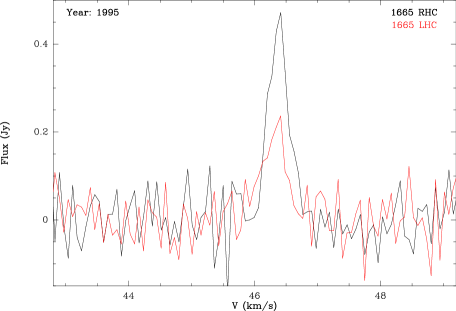
Figure 1: Average of the 4 OH 1665-MHz single-dish observations obtained with the NRT (over a period of 30 days, between mid-November and mid-December) around the MERLIN observations of the 28^th of November 1995.

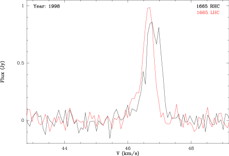
Figure 2: Average of the 5 OH 1665-MHz single-dish observations obtained with the NRT (over a period of 30 days, between mid-April and mid-May) around the MERLIN observations of the 4^th of May 1998.

1667 MHz
Faint 1667 MHz emission was detected intermittently. Figure 3 presents the detection made of this line, around the OH maximum of 1992 (at the optical phase +0.2) along with the corresponding 1665 MHz spectra for comparison. The figure is an average of the 3 NRT observations taken between the 1^st and the 10^th of October 1992 so as to increase the SNR (note that the number of spectra selected for the average for the 3 series of spectra presented in Figs 1, 2 & 3 was chosen so as to get a similar rms of 55-60mJy, bringing out of the noise rather faint but reasonably long-lasting components). The LHC and RHC 1667-MHz peaks have similar intensities and are both centred at V${}_{\rm peak}\sim+46.07$ km s^-1, which is roughly the mid-point between the 1665-MHz LHC and RHC spectra in 1992 and is $\sim$0.35 km s^-1 “bluer” than the 1665 MHz peak of the late-1995 cycle. With a separation of 965 days, this hints towards a similar velocity drift over a similar time interval as the one recorded between late-1995 and mid-1998.

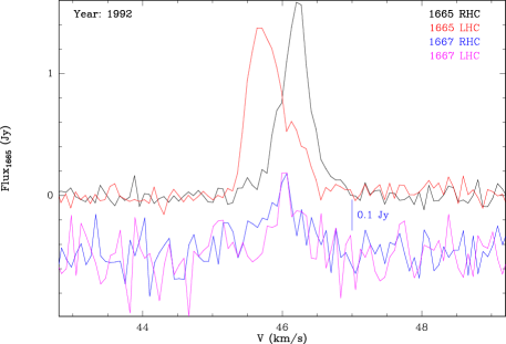
Figure 3: Average of the 3 OH 1665-MHz & 1667-MHz single-dish observations obtained with the NRT between the 1^st and the 10^th of October 1992 so as to increase the signal to noise. Note the difference in flux scale between the 1665 MHz spectra (given by the left-hand-side coordinate axis) and the 1667 MHz spectra (given by the vertical bar on the right-hand side of the LHC & RHC spectra themselves).

3.1.2 The MERLIN maps

Figure 4: 1665-MHz OH maser map of the sum of all the channels where emission has been detected in the Stokes $I$ datacube from the MERLIN observations taken on the 28^th of November 1995. The restoring beam (0.34610 $\times$ 0.14505 arcsec², PA=$+26.22$) is shown in the lower-left corner. The spectrum constructed from the Stokes $I$ datacube is shown in superimposition in the bottom-right corner of the map.

Figure 5: Same as for Fig. 4 but for the MERLIN 1665-MHz OH maser observations taken on the 4^th of May 1998. The restoring beam (0.32781 $\times$ 0.24763 arcsec², PA=$+28.66$) is shown in the lower-left corner while the spectrum constructed from the Stokes $I$ datacube is superimposed in the top-right corner of the map.

Two epochs of interferometric observations with MERLIN were taken in 1995 and 1998, 2 years and 5 months apart. For these 2 datasets, the full polarisation information was not retrievable. Since no (circularly-polarised) substructure can be seen in the maser components themselves, only the resulting Stokes $I$ maps are presented here in Figs 4 & 5. These maps have been created by summing up all the channels where emission has been detected in the final Stokes $I$ datacube. The spectra built from these datacubes are also presented. The comparison of the peak intensity of the MERLIN spectra with the NRT single-dish spectra (cf. Fig. 1) implies that no significant part of the signal was missed during the interferometric 1995 observations.

With the warning given in Section 3.1.1 regarding the peak intensities of the averaged spectrum presented in Fig. 2 being biased towards the mid-April spectra, the comparison of the Stokes $I$ peak intensity of the 1998 MERLIN spectra with that recorded mid-May by the NRT (i.e., the closest NRT spectra to the MERLIN observations which equate to F${}_{peak\;(Stokes\;I)}\sim 0.69$ Jy) indicates that at least 85% of the signal was recovered during the 1998 interferometric observations.

In 1995, two maser components were detected separated by about $1\arcsec$ (at RA_J2000=$02^{h}19^{m}20.7647^{s}$ and DEC_J2000=$-02^{\circ}58\arcmin 38.536\arcsec$ for the strongest, and RA_J2000=$02^{h}19^{m}20.7131^{s}$ and DEC_J2000=$-02^{\circ}58\arcmin 37.956\arcsec$ for the faintest), while only one maser component was detected in 1998 (at RA_J2000=$02^{h}19^{m}20.7687^{s}$ and DEC_J2000=$-02^{\circ}58\arcmin 39.182\arcsec$). The comparison of the proper-motion corrected positions of the 2 maser components detected in 1995 with the 1998 one is such that the strongest 1995 component is located the closest to the 1998 component. Between the 2 epochs of observations, the difference in position of the strongest maser component has been measured to be $\delta_{\rm RA}\simeq+58.5$ mas $\delta_{\rm Dec}\simeq-680$ mas, while a proper motion of $\delta{\rm PM}_{\rm RA}\simeq+22.5$ mas and $\delta{\rm PM}_{\rm Dec}\simeq-574$ mas is expected. This leads to an actual positional difference of $\simeq$110 mas ($\sim$13 AU) between them. Following the V_exp=f(period) relation for Miras of Sivagnanam et al. (1989), and taking into account the spread in this relation, a standard OH expansion velocity of 3-5 km s^-1 is expected for $o$ Ceti. The same maser component would then be expected to have travelled a linear distance of $\sim$1.5–2.5 AU radially outward over the 888 days separating the 2 MERLIN observations. This expected propagation is smaller by at least a factor of 5 than the measured separation between the 2 strongest maser components. Also, the measured separation is greater than the absolute positional uncertainty which means that if those 2 maser components are probing the same region of the shell, as expected since both epochs correspond to the same event evolving over a time interval of $\sim$10 yr, then the difference in position observed here represents a genuine snapshot of the propagation of the flare within the affected region, the disturbance speed being $\sim$25 km s^-1.

3.2 The flaring event of the 2010s

3.2.1 The single-dish NRT OH monitoring

We present here the status of the observations obtained during the 2009-2010 cycle, which corresponds to the first cycle of the 2010s’ OH flaring event. All 3 ground-state lines known to be potentially present towards O-rich evolved stars, that is the 2 main lines at 1665 and 1667 MHz and the satellite line at 1612 MHz were monitored. No emission was detected in either the 1667- or the 1612-MHz lines.

Figure 6 shows the average NRT spectrum of the first cycle of the 2010s’ OH flaring event observed in the 1665-MHz line. The average spectrum is made of all the spectra taken between December 2009 and February 2010 inclusive (corresponding roughly to the modified Julian day (MJD) interval [55170–55260]), that is the spectra with the highest SNR since encompassing the OH maximum. The velocity information of the first detection of OH emission in 1974 by Dickinson, Kollberg & Yngvesson (1975) and the overall velocity span observed during the 1990s’ flaring event (Gérard & Bourgois 1993) are represented by the red and green horizontal bars, respectively. The new emission is composed of 2 strongly polarised main spectral components (the strongest and faintest components are labelled Comp I and Comp II, respectively). It presents a profile and a velocity spread similar to what was observed in the 1990s’ flare but it is now centred at V$\simeq+47.1$ km s^-1 (and spans the velocity interval V=[$+46.4$,$+47.8$] km s^-1), while in the 1990s, the flaring emission was centred at V$\simeq+46$ km s^-1 (and spanned the velocity interval V=[$+45.3$,$+46.8$] km s^-1, cf. Gérard & Bourgois 1993, their Fig. 1). Note that Dickinson, Kollberg & Yngvesson (1975) report the following characteristics for their observation in the 1970s: V_peak=$+46.5$ km s^-1 with a line width $\Delta$V=0.5 km s^-1.

With only one peak observed in the OH spectrum, it is likely that only one side of the shell is experiencing the flare as standard Miras commonly exhibit a double-peak profile with a typical expansion velocity of few ($<$10) km s^-1 (Sivagnanam et al. 1989).

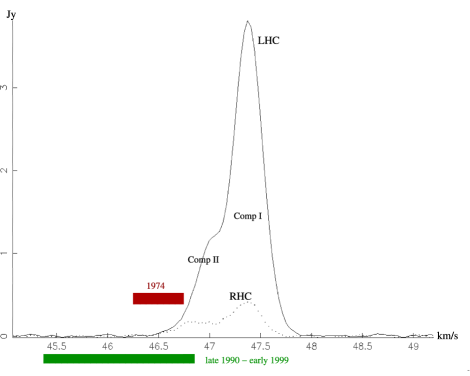
Figure 6: Average NRT spectra in the LHC (solid line) and RHC (dotted line) polarisations covering the period December 2009 – February 2010, (corresponding roughly to the MJD interval [55170–55260]) which encompasses the OH maximum of the first cycle of the 2010s’ OH flaring event. The red horizontal bar gives the velocity range of the OH emission recorded in 1974, and the green horizontal bar gives the OH emission velocity spread in 1990-1999. The 2 persistent spectral components observed are labelled Comp I and Comp II for the strongest and the faintest one respectively.

Figure 7 presents the variability curves of the individual components after Gaussian spectral decomposition both in RHC and LHC polarisations. Note that from MJD=55310, the signal decreased below the noise level for the rest of the cycle presented here. These main components all follow the cycle with the expected delay with respect to the optical light curve, which is of $\sim$70 days corresponding to an optical phase of +0.2.

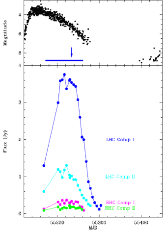
Figure 7: Top panel: $o$ Ceti’s optical lightcurve of the 2009 – 2010 cycle (data from AAVSO). Lower panel: Variability curves of the 1665-MHz individual components (Comp I and Comp II as identified in Fig. 6) after Gaussian spectral decomposition both in RHC and LHC polarisations. The horizontal bar shows the interval over which the NRT spectrum presented in Fig. 6 is averaged. The arrow indicates the date corresponding to the EVN-(e)MERLIN observations (taken at the optical phase +0.26). Note that from MJD=55310 the signal decreased below the noise level for the rest of the cycle presented here.

3.2.2 The EVN-(e)MERLIN maps

Figure 8 presents the pre-self-calibration map of the LHC emission of the 2010s’ flaring event, obtained with the EVN-(e)MERLIN array, just past the OH maximum, in February 2010 at the optical phase +0.26. It shows the dominating component which was used for self-calibration so as to improve the signal to noise of the datacube. Gaussian fitting of this component leads to an astrometric position of RA${}_{\rm J2000}=02^{h}19^{m}20.8091^{s}$, DEC${}_{\rm J2000}=-02^{\circ}58\arcmin 41.935\arcsec$. The purple and green crosses give the estimated positions of $o$ Ceti and its companion Mira B, respectively. These positions are extrapolated from Matthews & Karovska’s (2006) VLA imaging, taking into account the proper motion (van Leeuwen 2007). The 2010s’ flaring region is located $\sim$200$\pm$40 mas (i.e., $\leq$ 20$\pm$4 AU) east of $o$ Ceti.

From a 2-D Gaussian fitting of the ALMA band 3 & 6 continuum observations taken between the 17^th and 25^th of October 2014 and between the 29^th of October and the 1^st of November 2014 respectively, Wittkowski et al. (submitted) determined the position of Mira A to be $02^{h}19^{m}20.795016^{s}$ ($\pm 0.00006\arcsec$) $-02^{\circ}58\arcmin 43.03984\arcsec$ ($\pm 0.00007\arcsec$) and $02^{h}19^{m}20.795055^{s}$ ($\pm 0.00003\arcsec$) $-02^{\circ}58\arcmin 43.05078\arcsec$ ($\pm 0.00006\arcsec$)

for the Band 3 and Band 6 epochs, respectively. Taking into account the proper motion of $o$ Ceti (van Leeuwen, 2007), these newer sets of position agree within 20 mas to the one we inferred from Matthews & Karovska’s (2006) maps. Adding quadratically the uncertainties means that the relative position of the MERLIN/EVN-(e)MERLIN maser components relative to the position of $o$ Ceti has an overall uncertainty of 40 mas. We interpolated the position of Mira B relative to that of Mira A adopting the measurement values compiled by Planesas, Alcolea & Bachiller (2016). We adopted a conservative uncertainty of 40 mas, corresponding to the sum of the biggest individual-measurement uncertainty claimed by the authors and half the inferred positional shift in RA and DEC over the relevant period of the work presented here.

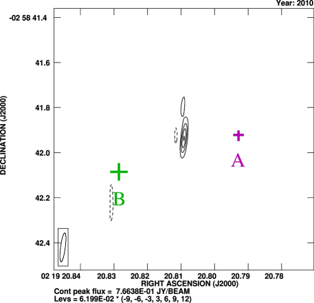
Figure 8: Phase-referenced pre-self-calibration image of the EVN-(e)MERLIN LHC map of the flare taken in February 2010 at the optical phase +0.26. The restoring beam (0.11770 $\times$ 0.02044 arcsec², PA=$-13.62$) is shown in the lower-left. The purple and green crosses give the estimated positions of $o$ Ceti and its companion Mira B, respectively. The positions of Mira A is extrapolated from Matthews & Karovska’s (2006) VLA imaging, taking into account the proper motion (van Leeuwen 2007). The position of Mira B is relative to that of Mira A and was inferred from the measurement values compiled by Planesas, Alcolea & Bachiller (2016). The size of the crosses represents the uncertainty of the absolute position of stars.

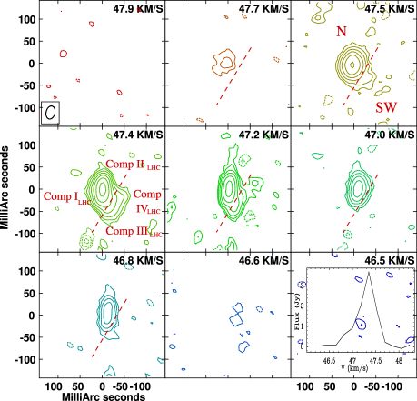
Figure 9: 1665-MHz LHC contour maps for all the channels where emission was detected in the EVN-(e)MERLIN observations. The restoring beam (0.03000 $\times$ 0.02000 arcsec² with a PA=$-13$) is shown in the lower-left corner of the top-left channel map. The contours are at ($-1$, 1, 2, 3, 5, 8, 10, 25, 35, 80) $\times$ 0.01828 Jy beam^-1. The spectrum constructed from the datacube is superimposed over the lower-right channel map. The dashed line marks the border between the northern (N) and the south-west (SW) groups of components.

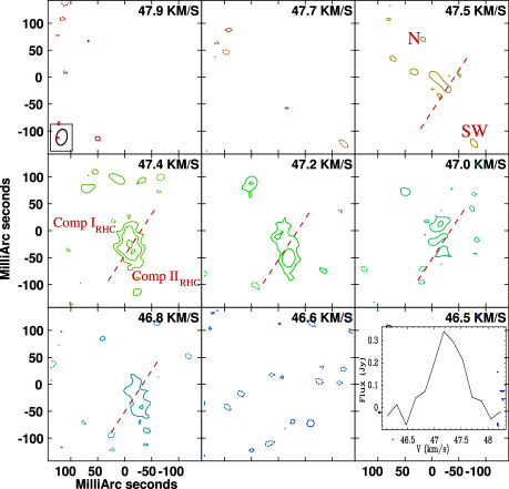
Figure 10: Same as Fig. 9 for the 1665-MHz RHC. The same restoring beam and contour levels have been used as given in Fig. 9.

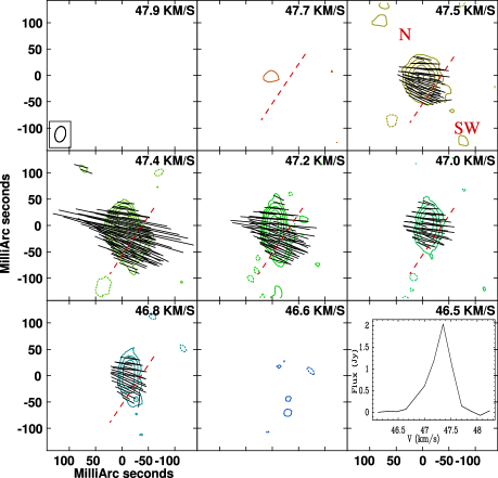
Figure 11: EVN-(e)MERLIN 1665-MHz Stokes I contour maps on which the polarimetric information is overlaid. Note that this shows only the relative linear PPAs as the observations of the PPA calibrator 3C286 were unfortunately unsuccessful. The length of a vector is proportional to the percentage of linear polarisation. As in Figs 9 & 10, the spectrum constructed from the datacube is superimposed over the lower-right channel map. The same restoring beam and contour levels have been used as given in Fig. 9.

Figures 9 & 10 present the post-self-calibration contour maps of all the channels where emission was detected in the LHC and RHC polarisations, respectively. Also shown, superimposed on the lower-right channel map is the spectrum constructed from the respective datacubes. The comparison of the profile and peak intensity of the EVN-(e)MERLIN spectra with the average NRT single-dish spectra (cf. Fig. 6) indicates that at least 90% of the signal has been recovered during the interferometric observations.

A close analysis reveals that in the LHC polarisation there are actually 2 main groups of components: 2 strong components which are barely 16 mas apart from each other (labelled group “N”) and 2 fainter components, $\sim$40 mas south-west of the 2 strong northern group of components (labelled group “SW”). For visualisation purpose, a dash line marking the separation between the “N” and “SW” groups is displayed in the figures for the channels where emission was detected. The 2 strong components in group “N” correspond to Comp I${}_{\rm\,LHC}$ & Comp II${}_{\rm\,LHC}$ as labelled in Figs 6 & 7. In this group of components, there is a gradual shift from the western component (Comp II${}_{\rm\,LHC}$) to the eastern one (Comp I${}_{\rm\,LHC}$), while the velocity increases over the entire velocity range covered by the LHC polarised emission. The “SW” group of components (which spectral signature is not apparent in the averaged spectra shown in Fig. 6 and that we shall label Comp III${}_{\rm\,LHC}$ & Comp IV${}_{\rm\,LHC}$) span over the much smaller velocity range V=[$+47.1$,$+47.6$] km s^-1 (cf. Table 1 presenting a summary of the velocity and location of the compoments). Due to the faintness of the signal in RHC polarisation, the structure of the rather compact emission is less well-defined. Yet, both Comp I${}_{\rm\,RHC}$ and Comp II${}_{\rm\,RHC}$ (as labelled in Figs 6 & 7) can be identified in Fig. 10. Comp I${}_{\rm\,RHC}$, spanning the velocity range V=[$+47.0$,$+47.6$] km s^-1, is located in the western part of group “N”. Comp II${}_{\rm\,RHC}$, spanning the velocity range V=[$+46.7$,$+47.4$] km s^-1 belongs to group “SW”. Gaussian fitting was used to measure precisely the position of the various components to search for possible Zeeman pairs. The criteria for a Zeeman pairing is a positional agreement to within the absolute positional uncertainty of ($35\times 10$) mas² (cf. Section 2.2.3). The Gaussian fitting reveals that in group “N”, with a positional agreement of ($16\times 8$) mas², the western component is actually a Zeeman pair made of Comp II${}_{\rm\,LHC}$ (centred at $V_{\rm II_{LHC}}\sim+47.0$ km s^-1) and its Zeeman counterpart Comp I${}_{\rm\,RHC}$ (centred at $V_{\rm I_{RHC}}\sim+47.4$ km s^-1). Note that the actual position of Comp II${}_{\rm\,RHC}$ is better visually guessed in the channel map $V=+47.0$ km s^-1 as, in particular in the channel map $V=+47.4$ km s^-1 it is hard to disentangle visually Comp I${}_{\rm\,RHC}$ and Comp II${}_{\rm\,RHC}$.

In group “SW”, Comp III${}_{\rm\,LHC}$ and Comp II${}_{\rm\,RHC}$ are also a Zeeman pair, but of much fainter intensity, preventing us to ascertain its velocity signature.

Table 1: Component characteristics summary

Component	aPeak Velocity or	Zeeman Pairing
Label	Velocity Range
	(km s-1)
Group “N”
Comp I${}_{\rm\,LHC}$	$V_{\rm Peak}\simeq+47.4$
Comp II${}_{\rm\,LHC}$	$V_{\rm Peak}\simeq+47.0$	Z1
Comp I${}_{\rm\,RHC}$	$V_{\rm Peak}\simeq+47.4$	Z1
Group “SW”
Comp III${}_{\rm\,LHC}$	[$+47.1$,$+47.6$]	bZ2
Comp IV${}_{\rm\,LHC}$	[$+47.1$,$+47.4$]
Comp II${}_{\rm\,RHC}$	[$+46.7$,$+47.4$]	bZ2

a: The peak velocity of the component is given when measurable with enough precision, else the velocity range of the component is given
b: The faintness of the signal does not allow the measurement of the component peak velocities with enough precision preventing to ascertain the velocity signature of this Zeeman pair

Figure 11 presents the Stokes I contour maps on which the polarimetric information is overlaid. Note that as the observations of the PPA calibrator 3C286 were unfortunately unsuccessful, the polarimetric vectors presented in the figure are not the absolute PPAs which are not retrievable. Only the difference in angles (i.e., the relative PPAs) are to be taken into consideration. Bearing this in mind, it is nonetheless clear that the distribution of the vectors of polarisation attests to an underlying ordered but relatively complex magnetic field. The EVN-(e)MERLIN polarised maps show that the vectors of polarisation associated with group “N” and group “SW” have PPAs differing by $~{}\sim 20^{\circ}$ hence revealing the intricacy of the magnetic field lines probed by the flaring OH maser emission down to a resolution of a few tenths of mas.

3.2.3 The single-dish Medicina and Effelsberg H₂O monitoring

Figure 12 presents a spectrum of the 22 GHz H₂O maser emission obtained in December 2009 with the Medicina antenna during the rise of the OH maser emission towards the maximum, on which the velocity range of the 2010s’ OH flare is also displayed. It is clear that both maser species are emitting in a similar velocity range. What is more, they both peak at a similar velocity.

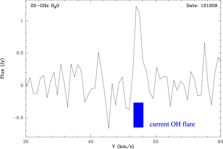
Figure 12: Medicina spectrum of the H₂O maser emission obtained in December 2009 during the rise of the OH maser emission towards the maximum (integration time: 20 min, resolution: 0.53 km s^-1; rms: 0.25 Jy). The width of the vertical bar gives the 2010s’ OH emission velocity spread.

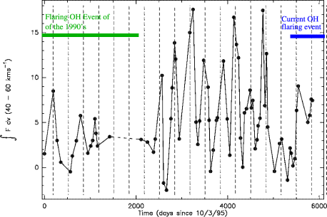
Figure 13: Variability curve of the 22-GHz water maser emission recorded from March 1995 until March 2011 at Medicina (68 spectra) and Effelsberg (6 spectra). Note: no observations were performed between the 01/03/1999 and 20/12/2000 represented by the nearly horizontal dashed line. The vertical dashed lines mark the 332-day optical period arbitrarily shifted to roughly coincide with peaks in the H₂O emission), which the water maser seems to follow quite well. The OH flaring events recorded during the time interval presented here are also displayed.

Figure 13 shows the variability curve of the 22-GHz water maser emission from March 1995 until March 2011 based on 68 and 6 spectra taken with the Medicina and Effelsberg telescopes respectively. The vertical dashed lines mark the 332-day optical period, which the water maser seems to follow quite well. Note though that the lines have been arbitrarily shifted to roughly coincide with peaks in the H₂O emission (and do not mark the actual optical minima or maxima). They serve as a guide to show that the optical period characterises reasonably well also the H₂O periodicity. Further detailed analysis of the H₂O variability characteristics, which is beyond the scope of this article, will be presented in Brand et al. (2017). Also displayed in the figure are the two OH maser flaring events of the 1990s and the 2010s. Interestingly, the comparison of the long-term variability of the 22-GHz H₂O maser emission with that of the OH maser activity towards $o$ Ceti, shows that OH flaring events seem to appear when the 22-GHz H₂O is relatively fainter.

4 Discussion

4.1 Location of the flaring regions

The 1995 MERLIN observations and the EVN-(e)MERLIN observations of the current 2010s’ flare were obtained 14 years 2 months apart. Therefore, a proper motion of $\delta{\rm PM}_{\rm RA}\simeq+0.132\arcsec$ and $\delta{\rm PM}_{\rm Dec}\simeq-3.36\arcsec$ is expected. The difference measured between the position of the maser component observed in the 2010s’ event and the strongest one in the 1995 map is $\delta_{\rm RA}\simeq+0.621\arcsec$ $\delta_{\rm Dec}\simeq-3.24\arcsec$, while it is $\delta_{\rm RA}\simeq+1.35\arcsec$ $\delta_{\rm Dec}\simeq-3.84\arcsec$ with respect to the faintest component of the 1995 map. The 2010s’ maser position is consequently offset from the positions of the stronger and fainter maser components observed in 1995 by $0.5\arcsec$ and $1.3\arcsec$, respectively. This is significantly greater than the expected distance travelled over 14 years by the same parcel of material in the CSE due to expansion, hence implying that the 1990s’ flaring emission and the 2010s’ one originate from 2 distinct regions (cf. also the discusion regarding the flare velocity properties in section 4.2).

Figure 14 presents the relative positions of the OH flaring region measured by the EVN-(e)MERLIN in February 2010 along with the MERLIN masers detected in 1995 and 1998 and the stars of the Mira AB system, taking Mira A as the reference position, and correcting all the positions for proper motion (cf. Table 2 for the calculated offsets). While the 2010s’ flaring event is clearly affecting the region located between Mira A and Mira B, the 1990s’ event affected only the part of the shell in the opposite side to Mira B.

Table 2: Offsets of the maser components and Mira B relative to $o$ Ceti

	Xoffset	Yoffset
	($\arcsec$)	($\arcsec$)
Mira B	+0.543	$-0.174^{*}$
MERLIN 95 strongest maser comp.	$-0.299$	+0.017
MERLIN 95 faintest maser comp.	$-1.078$	+0.596
MERLIN 98 maser comp.	$-0.269$	$-0.052$
EVN-(e)MERLIN maser spot	+0.240	$-0.014$

Reference position: extrapolated position of $o$ Ceti the 04^th of May 1998 inferred to be RA${}_{\rm J2000}=02^{h}19^{m}20.7860^{s}$, DEC${}_{\rm J2000}=-02^{\circ}58\arcmin 39.130\arcsec$
*: Relative position to Mira A, interpolated from the series of measurements compiled by Planesas, Alcolea & Bachiller (2016)

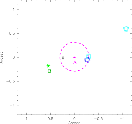
Figure 14: Relative positions of the OH flaring region measured by the EVN-(e)MERLIN in February 2010 (black), the MERLIN masers (light blue: 1995 / dark blue: 1998) and the stars of the Mira AB system (purple star: Mira A /green star: Mira B), taking Mira A as the reference position, and correcting all the positions for proper motion. Note that the size of the symbols represent the astrometric uncertainty of the given positions for the stars while for the masers, it represents their convolved sizes. The dashed-circle centred on $o$ Ceti and giving the distance to the centre of the strongest 1995 maser component has a radius of $0.3\arcsec$ ($\sim$30 AU).

In order to better constrain the exact position of the flaring regions in relation to Mira B, a more constrained determination of the orbital movement is needed. In particular, the ALMA observations of late October-early November 2014 lead to a most modern measurement of the separation of the Mira A and B of 0.472 arsec (corresponding to 43.4 AU at a distance of 92 pc) and a hint towards a decrease in separation (Vlemmings et al. 2015). Still, with this uncertainty in mind (i.e., $\sim$100 mas of uncertainty for the absolute positioning of Mira B), it is striking, that the strongest maser emission detected in the 3 epochs originate from a projected distance of less than 0.4$\pm 0.04\arcsec$ (that is less than 40$\pm$4 AU, taking into consideration the convolved size of the maser components while the dashed-circle in Fig. 14 gives the distance to the centre of the strongest 1995 maser component) from Mira A, with a hint of a potentially “deeper” OH flaring region on the side of the companion. Only a very faint maser component is found further out, $\sim 1.1\arcsec$ (i.e., $\sim$110 AU) away. This strongly suggests that the projected distances measured over these 3 independent epochs are a good estimation of the actual radius at which the recurrent flaring events appear, which is unusually close to the central star.

There is a relation between the OH radius and the mass-loss rate (and hence the shell thickness, Huggins & Glassgold 1982) as well as between the expansion velocity observed in the OH main lines of Miras and their period (Sivagnanam et al. 1989). So, one expects the OH (main-line) standard shell size to be roughly related to the period of the central Mira, which is indeed in agreement with the typical sizes found by mapping (Chapman, Cohen & Saikia 1991; Chapman et al. 1994). In particular, Chapman, Cohen & Saikia (1991) measured the radius of the loci of the strongest OH emission around U Ori, a thin-shell Mira with a similar period duration (368 days, Kukarkin et al. 1970) located at $\sim$306 $\pm$61 pc (Mondal & Chandrasekhar (2005) using Whitelock & Feast’s (2000) Period-Luminosity relation), to be $0\aas@@fstack{\prime\prime}21-0\aas@@fstack{\prime\prime}24$. From these mapping results, we can infer the typical radius at which the bulk of the standard OH main-line maser emission for a Mira having a period of about one year is expected to arise from, to be about R${}_{peak}\sim$100 AU (with fainter emission extending at smaller and greater radius around the R_peak) in agreement with the location of the fainter remote OH maser component detected here.

The faint more distant maser component observed in 1995, is then most likely coming from the standard OH shell. The fact that only one such maser component was observed and only at one epoch, suggests that further out in the CSE, in particular at the location of the standard OH envelope, the conditions for maser emission do not seem to be optimal. Furthermore, we note that this remote faint maser component is located on the opposite side of the shell with respect to the companion Mira B. The presence of the close companion is most likely to strongly perturb the standard CSE part of the shell to the side closer to it, inhibiting maser emission in these regions.

4.2 Flare propagation and velocity drift

The propagation of the flaring region during the 1990s’ event was happening at a speed of V$\sim$25 km s^-1 with a hint of a clockwise propagation. With such a velocity and direction of propagation, the 1990s’ flaring region would be expected to be roughly south of $o$ Ceti after the 12.5 years separating the 1990s’ and 2010s’ flaring events.

Due to its binary nature, $o$ Ceti is expected to undergo an orbital motion around the barycentre of the system. Baize (1980) proposed a first estimation of the orbital elements of the system which have been recalculated more recently by Prieur et al. (2002), in the light of new speckle observations of $o$ Ceti. Nevertheless, and as pointed out by the latter authors, since even the sum of the masses is unknown and the trajectory is still poorly sampled, the orbital elements of the binary system can not be tightly constrained. The observed velocity drift of $\sim$[0.27 – 0.35] km s^-1 in 888 days of the peak of the maser emission (that is $\sim$[0.11 – 0.14] km s^-1 per year), could be the signature of the orbital motion of Mira A around the barycentre of the system. Due to the play of intensity of the spectral components during time, there is an indication that the velocity drift of the emission peak is most likely higher than the intrinsic drift of each individual spectral component. A more refined value of the intrinsic velocity drift would require the complete analysis of the long term variability characteristics of the individual spectral component, which is beyond the scope of this paper. Such an analysis will be presented in a subsequent paper. Bearing in mind this latter warning and that a wide range of parameters is possible in terms of orbital parameters, adopting the most recent orbital period determination of Prieur et al. (2002; P$\sim$500 yr), a total mass of the system of 3.0 M_⊙, a typical Mira mass of 1.0 M_⊙ for $o$ Ceti, a deprojected separation of $\sim$85.6 AU between the 2 stars would lead to an intrinsic acceleration of $\sim$0.05 km s^-1 yr^-1 around the barycentre of the system for $o$ Ceti. Note that the total mass of 3.0 M_⊙ adopted here would not necessarily preclude Mira B from being a white dwarf, as the 2.0 M_⊙ represents the overall counterpart mass of the binary system, corresponding to Mira B and the surrounding material of the binary system.

4.3 Front or back part of the CSE?
A stellar velocity determination issue

Several AGB stars show a double-component profile in CO, composed of a relatively strong narrow component superimposed on a fainter and broader component, with both components centred on the same velocity (Knapp et al., 1998; Winters et al 2003). Such a profile is well constrained by a two-component parabolic fit and is interpreted by the aforementioned authors as a “double-wind” signature (i.e., the signature of 2 steady winds). $o$ Ceti is one of the stars that show 2 components in both its CO(3$-$2) and CO(2$-$1) profiles. But, since both lines clearly lack the red-shifted emission of the putative broad component, their profiles do not seem to be well constrained by such a composite narrow-broad component model. Assuming the validity of this model for $o$ Ceti – that is the existence of a broad component centred at the same central velocity as the narrow component – would imply that the red part of the broad component is missing, advocating for a highly asymmetrical “external” shell. Another possible interpretation which could account for the asymmetric line profile observed in the case of $o$ Ceti, has been put forward by Josselin et al. (2000). They mapped the CO(2$-$1) with the IRAM interferometer and also obtained optical spectroscopic observations of the KI lines in an attempt to detect the faint outer parts of the CSE. They propose the existence of a spherical shell disrupted by a bipolar outflow. The idea of a possibly bipolar CSE was previously proposed by Knapp & Morris (1985).

The non-symmetrical two-component nature of the CO profiles of $o$ Ceti reveals the complexity of its CSE with clear signs of asymmetry present even in the outermost part, but it also makes the determination of the stellar velocity and the final expansion velocity more problematic. Knapp & Morris (1985) estimate the stellar velocity from their CO(1$-$0) spectra to be V$=+46.8\pm 0.1$ km s^-1. Knapp et al. (1998), using a two-component parabolic fit (but not forcing the broad and narrow components to have the same central velocity) estimated the central velocity of the 2 components of the CO(3$-$2) emission to be V$=+46.6\pm 0.2$ km s^-1 and V$=+46.0\pm 1.0$ km s^-1 for the narrow and broad components respectively. Winters et al. (2003), also using a composite parabolic fit (but imposing a single central velocity for both the narrow and broad components of the profile), estimated the stellar velocity to be V$=+46.0$ km s^-1 and V$=+46.75$ km s^-1 from the CO(1$-$0) and the CO(2$-$1) profiles respectively (note that no uncertainties are given for these estimations, but a step of 0.25 km s^-1 has been used for the fits; Le Bertre, private communication). Considering all these estimations and their attached uncertainties, this leads to a rather loosely constrained stellar velocity, within the range [$+45.0$,$+47.0$] km s^-1 (cf. Fig. 15).

Note that independent inference of the systemic velocity from the inner part of the CSE (few R_∗) via SiO emission, adopted to be 45.7 $\pm$ 0.7 km s^-1 (Cotton et al. 2006) or more recently of $46.7$ km s^-1 by Wong et al. (2016), based on complex asymmetrical profiles, produce a similar range for the stellar velocity of $o$ Ceti.

With such a velocity range, encompassing that of the 1990s’ (and the mid-1970s’) flaring one, it is currently not possible to decide whether the flare in the 1990s and that of the mid-1970s (within the range V$\simeq$ [$+46.4$,$+46.9$] km s^-1 and centred at $+46.5$ km s^-1, respectively) emanates from in front or behind the star. Nonetheless, with a velocity range for the current 2010s’ flare (V$\simeq$[$+46.5$,$47.9$] km s^-1) it is likely that it is located in the back part of the shell.

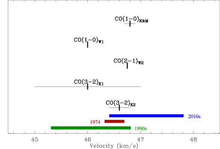
Figure 15: Diagram showing the various estimates of the stellar velocity from CO measurements and the OH maser velocity spread observed in 1974 (Dickinson, Kollberg & Yngvesson 1975), the 1990s and the 2010s. Uncertainties for the CO velocities are represented by horizontal bars. “K&M” stands for Knapp & Morris (1985), “K” stands for Knapp et al. (1998) and “W” stands for Winters et al. (2003). Note that the 2 values, “K1” and “K2” from Knapp et al. (1998) come from the same transition due to the two-component parabolic fit used by the authors to account for the spectral profile; though a similar two-component parabolic fit was also used by Winters et al. (2003) they used a fixed stellar velocity within a given transition. Note also that Winters et al. (2003) do not provide any uncertainties, but a step of 0.25 km s^-1 has been used for the fits (Le Bertre, private communication).

4.4 Comparison with previously recorded flaring events

So far, 6 other flaring events in thin-shell Miras have been recorded. The first record of such an event was made towards U Ori at 1612 MHz (Jewell, Webber & Snyder, 1981). Five other events were then recorded, at 1612 MHz towards U Her and R LMi, and in the main lines towards X Oph, R Leo, and R Cnc (Etoka & Le Squeren, 1996, 1997). A study based on all 6 objects was presented in Etoka & Le Squeren (1997). All 6 objects are found in a delimited portion of the [$60-25$] vs [$25-12$] IRAS colour-colour diagram where the bulk of non-OH oxygen-rich Miras are found. Even though the duration of the flares varies from a few months to several years, they are all characterised by a very short rise time. The flaring feature is always characterised by $|$V${}_{\rm star}-$V${}_{\rm flare}|<$ V${}_{\rm OH\;exp}$ (where V_flare is the peak velocity of the flaring feature, V${}_{\rm OH\;exp}$ is the standard OH expansion velocity and V_star the stellar velocity) which is clearly related to the [$25-12$] colour. The flaring emission shows substantial polarisation.

The OH flaring features in $o$ Ceti also show a strong polarisation. Due to the unusual nature of its OH emission, only observed as flaring events, a direct estimation of $o$ Ceti’s standard OH expansion velocity is not possible. The Sivagnanam et al. (1989) Velocity-Period relation implies a V${}_{\rm OH\,exp}\sim$3–5 km s^-1 for the period of $o$ Ceti (cf. Section 3.1.2). Chapman et al. (1991) estimated a V${}_{\rm OH\,exp}\sim$ 7 km s^-1 for U Ori. As noted previously, U Ori and $o$ Ceti have about the same period and hence should have a comparable expansion velocity. Knowing that the terminal expansion velocity of the CSE of $o$ Ceti, measured in the CO transitions, is only V${}_{\rm CO\,exp}\sim~{}6\pm 0.2$ km s^-1 (Knapp & Morris 1985) and that a small acceleration is still present at the location of the OH shell of Miras (e.g., Chapman et al. 1994), it is likely that for $o$ Ceti V${}_{\rm OH\;exp}\simeq$[4 – 5] km s^-1. This means that the flaring emission of $o$ Ceti is also characterised by $|$V${}_{\rm star}-$V${}_{\rm flare}|<$ V${}_{\rm OH\;exp}$ since $|$V${}_{\rm star}-$V${}_{\rm flare}|<$ 3 km s^-1, regardless of the actual stellar velocity (cf. Fig 15).

Figure 16 is the adapted Fig. 10 of Etoka & Le Squeren (1997) showing the [$60-25$] vs [$25-12$] IRAS colour-colour diagram of the nearby Miras (distance $<$ 1 kpc) with the location of all the flaring Miras indicated including $o$ Ceti. It shows the locations of “non-OH” Miras, that is the Miras which have not been detected in any of the ground-state OH maser transitions, the “Type I” Miras which are emitting predominantly in the 1665/67 MHz main lines and the “Type II” Miras, which have thicker CSEs and show their strongest emission in the 1612-MHz satellite line.

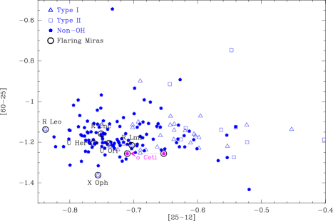
Figure 16: Adapted from Fig. 10 of Etoka & Le Squeren (1997) showing the [$60-25$] vs [$25-12$] IRAS colour-colour diagram of the nearby Miras (distance $<$ 1 kpc) with the location of all the flaring Miras indicated including $o$ Ceti. “Type I” stands for Miras which are emitting predominantly in the 1665/67 MHz main lines; “Type II’ stands for Miras which show their strongest emission in the 1612-MHz satellite maser line and “non-OH” stands for Miras which have not been detected in any of the ground-state OH maser transitions. Note that 2 positions are given for $o$ Ceti in this diagram. The “redder” one corresponds to the uncorrected value as calculated from the fluxes given in the IRAS Catalogue (i.e., corresponding to the overall binary system), while the “bluer” value is corrected for the mid-infrared excess identified by Ireland et al. (2007) and interpreted by the latter authors as being due to the accretion disk heated by Mira A (cf. text). The arrow shows the direction of the correction.

It has to be noted though that the fluxes given in the IRAS catalogue correspond to the overall Mira AB system and hence comprise also an excess of contribution due to the presence of the 2 stars in the beam, making $o$ Ceti look slightly “redder” than it actually is. Ireland et al. (2007) performed some mid-infrared observations of the Mira AB system and interpreted the mid-infrared excess they observed as coming from an optically-thick accretion disk heated by Mira A. Using the model fits of their work, constraining the SED of this disk (associated with Mira B), between 0.35 and 18.3 $\mu$m and doing a simple extrapolation to 25 $\mu$m, one can estimate its contamination into the IRAS measurements at 12 and 25 $\mu$m. This leads to a corrected [25-12] IRAS colour ranging between -0.690 to -0.710 (as opposed to an uncorrected value of -0.653). Adopting such a correction, the [$25-12$] IRAS colour for $o$ Ceti is indeed in agreement with the identified “flaring Mira area” of Etoka & Le Squeren’s (1997) former work.

Figure 17 presents the adapted Fig. 11 of Etoka & Le Squeren (1997) showing the relation found between $|$V${}_{\rm star}-$V${}_{\rm flare}|$ and the [$25-12$] IRAS colour of the flaring Miras, with the location of $o$ Ceti in this diagram. The actual location of $o$ Ceti in this diagram is rather poorly constrained due to, on the one hand, the contamination of its [$25-12$] colour by its companion Mira B and, on the other hand, its poorly constrained stellar velocity. This is illustrated in the diagram by the 2 vertical lines taking into account these 2 effects. Considering the decontaminated [$25-12$] colour brings $o$ Ceti to a better agreement with the [$25-12$] vs $|$V${}_{\rm star}-$V${}_{\rm flare}|$ relation observed for the rest of the flaring Miras. Yet, the location of $o$ Ceti in this diagram indicates that its $|$V${}_{\rm star}-$V${}_{\rm flare}|$ value is smaller than anticipated from the relation, even for the most optimistic decontaminated [$25-12$] colour. This hints at an even deeper location of the flaring region. A possible interpretation of this is that it reflects the influence of the companion “carving” even deeper the flaring zone in the side of the shell where it resides, by supplying an extra amount of anisotroptic UV radiation.

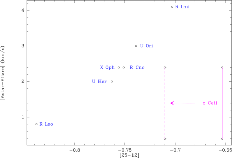
Figure 17: Adapted Fig. 11 of Etoka & Le Squeren (1997) showing the relation found between $|$V${}_{\rm star}-$V${}_{\rm flare}|$ and the [$25-12$] IRAS colour of the flaring Miras and the location of $o$ Ceti in this diagram. Note that the actual location of $o$ Ceti in this diagram is rather poorly constrained due to, on the one hand, the contamination of its [$25-12$] colour by the presence of its companion Mira B and, in the other hand, its poorly constrained stellar velocity, illustrated here by the 2 vertical lines taking into accounts these 2 effects.

4.5 OH luminosities of flaring Miras

Nguyen-Q-Rieu et al. (1979) performed a statistical study towards 48 Miras to determine their OH intrinsic luminosities. They find that the Type-I OH intrinsic luminosity ranges from $\sim$5$\times 10^{15}$ to $\sim$5$\times 10^{17}$ Watt Hz^-1, while the Type-II OH intrinsic luminosity ranges from $\sim 10^{17}$ to $\sim$5$\times 10^{18}$ Watt Hz^-1. A more recent statistical study performed over the $>$2000 Galactic stellar sources known to be OH emitters (i.e., including Miras, SRs and OH/IR stars) from the catalogue of Engels & Bunzel (2015) was made by Etoka et al. (2015). Discarding the few low- and high-luminosity outliers in the distribution, the upper limits found in this new study agree with those of Nguyen-Q-Rieu et al. (1979) but the lower limits extend much further for both main-line and 1612-MHz satellite-line emitters by more than 2 orders of magnitude. Taking the mean intensity of the OH emission observed towards each flaring Mira, leads to an OH intrinsic luminosity ranging from $\sim$2$\times 10^{12}$ to $\sim$3.5$\times 10^{13}$ Watt Hz^-1, with that of $o$ Ceti being the lowest. This range of luminosities corresponds to the lower part of the distribution in Etoka et al. (2015) and might be taken as typical for the flaring stellar maser population. This Mira group represents then the lower range of the Mira population both in terms of luminosity and mass-loss rate. From these 2 characteristics and their location in the [$60-25$] vs [$25-12$] IRAS colour-colour diagram, i.e., in the midst of the non-OH Miras and the edge of the Type-I Miras, one plausible interpretation is that this group represent a transition between the 2 populations, pinpointing the lower limits in terms of physical properties needed for the OH maser to be present in the CSE.

4.6 Polarisation and underlying magnetic field structure

Etoka & Le Squeren’s (1996, 1997) spectral records of the LHC and RHC spectra of the previous flaring events occuring in the 1665-MHz transition clearly show hints of Zeeman splitting signatures but a confirmation and accurate measurement of the associated magnetic field strength was not possible since no maps of these events were available.

Though the absolute polarisation angle associated with the maser components could not be retrieved, preventing us from making a detailed analysis of the underlying magnetic field structure, it is clear from the distribution of the linear vectors of polarisation presented in Fig. 11 that the masers in $o$ Ceti trace an ordered but relatively complex magnetic field structure. The Zeeman pair detected in group “N” (cf. Table 1), at a distance from the star $\sim$200$\pm$40 mas (i.e., $\leq 20\pm 4$ AU), leads to a magnetic field of $B\sim+0.68$ mG, using the Zeeman splitting coefficient given by Davies (1974).

The high polarisation along with the erratic variability behaviour observed in the OH main-line flaring Miras is reminiscent of what is observed towards semiregular variable stars (Etoka et al. 2001; Szymczak et al. 2001). This type of stars is characterised by light curves less regular than that of Miras and the variation in their optical amplitudes is less than 2.5^m (Kholopov et al. 1985). They have infrared properties quite close to those of Miras emitting predominantly in the 1665/67 MHz main lines (i.e., the “Type-I” maser emitters). Analysis of their long-term OH maser emission variability and polarisation properties suggests that these characteristics are due to transient instabilities in their hot and thin CSEs (Etoka et al. 2001) where turbulence effects in the circumstellar magnetic field as well as magnetic field structural change are thought to occur (Szymczak et al. 2001).

4.7 Implication of the flare location with respect to the standard (OH) CSE model

From a statistical analysis of all the Miras previously recorded to have exhibited OH flaring events, Etoka & Le Squeren (1997, cf. also Section 4.4) concluded that the flaring emission is likely to originate from a region closer to the star than the distance at which OH maser emission in the standard model comes from. As mentioned in Section 3.2.3, the velocity peak and spread of the OH flaring emission and the 22-GHz H₂O are the same. This additional clue strongly supports the suggestion that the OH maser flaring emission observed here indeed originates from a region closer to the star than the standard OH maser CSE distances, in agreement with the findings of Etoka & Le Squeren (1997). Furthermore, as also mentioned Section 3.2.3, the long term monitoring of the 22-GHz H₂O maser emission shows that OH flaring events seem to appear when the 22-GHz H₂O is relatively fainter. A tentative explanation for this behaviour is that it is the signature of an enhanced OH production by photodissociation of H₂O which translated itself by a decrease of the water maser emission.

OH flaring events close to the central star only seem to occur in thin-shell Miras, indicating that the physical conditions for the masers to occur in these more internal zones are not fulfilled for thick-shell stars, possibly due to a non-favourable combination of temperature and/or density and/or pumping conditions.

Goldreich & Scoville (1976) and Huggins & Glassgold (1982) studied the physical properties of the CSE, demonstrating the importance of the ambient interstellar UV radiation in the production of OH molecules by photodissociation of H₂O. Huggins & Glassgold (1982) show the variation of the peak of the OH density profile formed by photoproduction with respect to the mass-loss rate and the importance of H₂O shielding in this process. While Goldreich & Scoville (1976) show that such a process delivers an important source of OH in the outer part of the CSE, their results also show that a high abundance of OH is expected in the CSE close to the star (cf. their Fig. 4, though admittedly their models are more adequate for OH/IR objects due to the high mass-loss rates adopted: $3\times 10^{-5}$ M_⊙ yr^-1).

Moreover, Cimerman & Scoville (1980) studied the possible importance of direct stellar radiation at 2.8 $\mu$m for the pumping scheme of OH maser lines (particularly effective for the main lines) in late-type stars. Using Goldreich & Scoville (1976) CSE models to test this scheme, Cimerman & Scoville suggest the existence of two zones of high OH emissivity with such a pumping mechanism where IR pumping plays a more significant role for the zone nearer to the star. Also, Collison & Nedoluha (1993) stress that the NIR pumping scheme proposed by Cimerman & Scoville (1980) can operate at significantly lower column densities of OH than the FIR pumping scheme.

While some faint 1667 MHz emission was observed during the 1990s’ event, emission at that frequency was not detected during the time interval covering the current 2010s’ flaring event presented here. The fact that 1665 MHz is excited while 1667 MHz is only sporadically observed is in favour of a denser or/and warmer environment. Indeed, from a statistical study of main-line emission towards Miras, Sivagnanam et al. (1989) show that the expansion velocities at 1665 and 1667 MHz are such that $\Delta$V${}_{1667}>[1.1-1.3]\Delta$V₁₆₆₅, indicating that acceleration is still present at the location where these maser transition occur and that 1667-MHz maser emission extends further out in the OH shell than the 1665-MHz maser emission (confirmed by mapping by e.g. Chapman et al. 1991). Furthermore, models (Elitzur 1978, Bujarrabal et al. 1980) show that higher gas temperature and density are more favourable to 1665-MHz maser emission implying that 1665-MHz maser emission is expected to be found down to a slightly more internal radius than 1667-MHz emission.

On the whole, the different positions of the OH masers between 1995 and 2010 (cf. Fig. 14) fall within a circle of radius $0.3\arcsec$, comparable with the SiO emission presented in Wong et al. (2016). Even the weak OH feature at $1\arcsec$ observed in 1995, seems to have a counterpart in the extended SiO emission. Also, we incidentally note that the excited H₂O transition at 232.67 GHz, mapped by ALMA, with an excitation energy $E_{up}/k\sim 3462$ K (Wong et al. 2016), hence tracing the warm H₂O layer, is confined within a much smaller radius of $\leq 0.1\arcsec$ from O Ceti than the OH flaring region.

4.8 Role of binarity in the flaring events towards $o$ Ceti

Danchi et al. (1994) measured the inner radii of the dust shell of a sample of 13 late-type stars, including $o$ Ceti, at 11.15 $\mu$m. They found two classes of stars. The group which $o$ Ceti belongs to, is the one for which the stars have their dust shells very close to the photosphere ($\sim$3 stellar radii for $o$ Ceti). They observed $o$ Ceti at a wide range of optical phases and with 3 different baselines, one of which (the 13 m baseline for which the position angle of PA=113^∘) is virtually aligned with the Mira AB axis (PA=$112^{\circ}\pm 1^{\circ}$, Karovska, Nisenson & Beletic 1993) and shows visibilities that hint at a smaller radius than for the other baselines. The authors also notice a similar signature of asymmetry in the TiO, which peaks closer to the star on the side illuminated by the companion Mira B.

Similarly, Lopez et al. (1997) performed visibility observations at  11 $\mu$m towards $o$ Ceti during a $\sim$7-year period, in the Mira-AB axis direction, which stress the non-spherical and evolving clumpy structure of the dust shell around $o$ Ceti. They even suggested that the formation of a new clump of dust could be linked to the OH flaring events observed in the 1990s by increasing temporarily the far-infrared emission which is known to operate as a common pump of the OH ground-state main lines (i.e., 1665 & 1667 MHz). Finally, very recent mapping of the CO emission around the Mira AB system with ALMA (Ramstedt et al. 2014) revealed the presence of a bubble, which the authors tentatively suggest is created by the wind of Mira B and blown into the expanding envelope of Mira A.

The general flaring characteristics observed for $o$ Ceti are similar to those observed for flares in isolated Miras in terms of IRAS colour-colour properties, velocity range in relation to the stellar velocity, spectral characteristics and polarisation behaviour as described by Etoka & Le Squeren (1997), which are quite distinct from what is observed towards standard Miras (Etoka & Le Squeren 2000). These common characteristics suggest that the flaring locations in terms of radius in the CSE is similar for all these events and all indicate that these regions of transient OH maser activity are distinct from the standard OH maser zone. Yet, in the case of $o$ Ceti there are also hints (e.g., the nature of the companion itself, asymmetrical emission in e.g. the CO and TiO, and the relatively small $|$V${}_{\rm star}-$V${}_{\rm flare}|$ value) that the presence of the companion is playing a role in the flares, most probably in producing “episodic” H₂O photodissociation in preferential regions.

5 Summary and Conclusions

We have presented the analysis of the onset of the new 2010s’ flaring event currently undergone by $o$ Ceti and compared its characteristics with those of the 1990s’ flaring event, based on a series of single-dish and interferometric complementary observations both in OH and H₂O, obtained with the NRT, Medicina and Effelsberg telescopes and the MERLIN and EVN-(e)MERLIN arrays. We also compared the overall characteristics of $o$ Ceti’s recurring flaring events with those which have been observed towards other thin-shell Miras and summarized by Etoka & Le Squeren (1997).

The NRT monitoring shows that the spectral profile of the 1665-MHz flaring emission of $o$ Ceti is comprised of a set of 2 main persistent components both in the LHC and RHC polarisations. For the 2010s’ flaring event period presented here, the well-sampled monitoring shows that the maser emission follows the optical light curve variation with a delay of $\sim$70 days, corresponding to a phase delay of +0.2 as is typically observed towards variable Miras. While the spectral profile and the velocity spread observed in the 1990s’ and 2010s’ event are simliar (i.e., consisting of 2 main spectral components with an overall velocity spread of 1.5 km s^-1), the central velocity differs by $\sim$1 km s^-1 between the 2 events. A velocity drift of $\sim$0.27–0.35 km s^-1 in $\sim$900 days of the 1665-MHz emission peak was observed during the 1990s which could be the signature of the movement of $o$ Ceti with respect to the barycentre of the binary system.

The multi-epoch mapping during the 1990s’ event showed that the flaring region is not static but actually slowly propagates within the affected zone, at a speed of $\sim$25 km s^-1.

Though both OH main lines are generally observed in standard Miras, only very weak 1667-MHz non-polarised emission was observed intermittently during the 1990s’ event.

During the 2010s’ flaring event, the contemporary monitoring of the 22 GHz H₂O emission and the flaring OH maser emission revealed that emission of both species have a similar velocity range and peak at a similar velocity. The monitorings also revealed that OH flaring events seem to appear when the 22-GHz H₂O is relatively faint. This is interpreted as being due to a higher OH production due to an enhanced photodissociation of H₂O.

The 2010 high angular resolution EVN-(e)MERLIN maps revealed the presence of 2 main groups of components. The polarised information of these data allowed us to infer that the flaring region is associated with a $B\sim+0.68$ mG relatively complex magnetic field.

While the current 2010s’ flaring event is located about $\sim$240$\pm$40 mas (i.e., $\leq 24\pm 4$ AU) east of $o$ Ceti between the 2 stars of the binary system, in the 1990s it was located at a similar distance from $o$ Ceti but on the other side of the star. Taking the 2 epochs into consideration, this leads to a radius for the flaring zone of less than $\sim$400$\pm$40 mas (i.e., $\leq 40\pm 4$ AU), with a hint of a potentially “deeper” OH flaring region in the side of the companion.

The general flaring characteristics in terms of infrared properties, velocity of the flaring components (compared to the OH standard expansion velocity expected for these stars) and polarimetric behaviour, are similar to those recorded towards 6 other thin-shell Miras. The OH intrinsic luminosity deduced from the overall sample of flaring Miras ranges from $\sim$2$\times 10^{12}$ to $\sim$3.5$\times 10^{13}$ Watt Hz^-1, with that of $o$ Ceti being the lowest. This range of luminosities might be taken as typical for the flaring stellar maser population. $o$ Ceti’s first multi-epoch interferometric mapping of such events confirms the unusually short radius at which such events occur and hence the suggestion brought by Etoka & Le Squeren (1997) that OH flaring zones in thin-shell Miras are located closer to the star than the standard-OH maser-emission zone. A possible explanation of such maser zones could reside in the pumping scheme at play, with the predominance of NIR pumping for eruptive zones of thin-shell Miras, which works at lower column densities of OH than the FIR pumping known to be the main pumping scheme for the standard OH maser zone.

References

- [Baize 1980] Baize P., 1980, A&AS, 39, 83
- [Bowers & Johnston 1994] Bowers P.F., Johnston K.J., 1994, ApJS, 92, 189
- [Brand et al.2017] Brand J., Winnberg A., & Engels D., 2017, in preparation
- [Bujarrabal et al. 1980] Bujarrabal V., Guibert J., Nguyen-Q-Rieu, Omont A., 1980, A&A, 84, 311
- [Chapman, Cohen & Saikia 1991] Chapman J.M., Cohen R.J., Saikia D.J., 1991, MNRAS, 249, 227
- [Chapman et al. 1994] Chapman J.M, Sivagnanam P., Cohen R.J., Le Squeren A.M., 1994, MNRAS, 268, 475
- [Cimerman & Scoville 1980] Cimerman M., Scoville N., 1980, ApJ, 239, 526
- [Collison & Nedoluha 1993] Collison A.J., Nedoluha G.E., 1993, ApJ, 413, 735
- [Condon 1997] Condon J.J., 1997, PASP, 109, 166
- [Cotton et al. 2006] Cotton W.D. et al. 2006, A&A 456, 339
- [Danchi et al. 1994] Danchi W.C., Bester M., Degiacomi C.G., Greenhill L.J., Townes C.H., 1994, AJ, 107, 1469
- [Davies 1974] Davies R.D., 1974, in Kerr F. J., Simonson S. C., eds, Proc. IAU Symp. 60, Galactic Radio Astronomy. Reidel, Dordrecht, p. 275
- [Dickinson, Kollberg & Yngvesson 1975] Dickinson D.F., Kollberg E., Yngvesson S., 1975, ApJ, 199, 131
- [Elitzur 1978] Elitzur M., 1978, A&A, 62, 305
- [Engels & Bunzel 2015] Engels D. & Bunzel F., 2015, A&A, 582A, 68
- [Etoka et al. 2015] Etoka S., Engels D., Imai H., Dawson J., Ellingsen S., Sjouwerman L., van Langevelde, H., PoS(AASKA14)125, 2015, aska conf, 125
- [Etoka & Diamond 2004] Etoka S., Diamond P.J., 2004, MNRAS, 348, 34
- [Etoka et al. 2001] Etoka S., Błaszkiewicz L., Szymczak M., Le Squeren A.M., 2001, A&A, 378, 522
- [Etoka & Le Squeren 2000] Etoka S., Le Squeren A.M., 2000, A&AS, 146, 179
- [Etoka & Le Squeren 1996] Etoka S., Le Squeren A.M., 1996, A&A, 315, 134
- [Etoka & Le Squeren 1997] Etoka S., Le Squeren A.M., 1997, A&A, 321, 877
- [Gérard & Bourgois 1993] Gérard E., Bourgois G., 1993, LNP, 412, 365
- [Goldreich & Scoville 1993] Goldreich P., Scoville N.Z., 1976, ApJ, 205, 144
- [Habing 1996] Habing H.J., 1996, A&AR, 7, 97
- [Huggins & Glassgold 1982] Huggins P.J., Glassgold A.E., 1982, AJ, 87, 1828
- [Ireland et al. 2007] Ireland M.J., Monnier J.D., Tuthill P.G., Cohen R.W., De Buizer J.M., Packham C., Ciardi D., Lloyd J.P., 2007, ApJ, 662, 651
- [Jewell et al. 1981] Jewell P.R., Webber J.C., Snyder L.E., 1981, ApJ, 249, 118
- [Karovska, Nisenson & Beletic 1993] Karovska M., Nisenson P., Beletic J., 1993, ApJ, 402, 311
- [Karovska et al. 1997] Karovska M., Hack W., Raymond J., Guinan E., 1997, ApJ, 482, L75
- [Knapp & Morris 1995] Knapp G.R., Morris M., 1985, ApJ, 292, 640
- [Knapp et al. 1998] Knapp G.R., Young K., Lee E., Jorissen A., 1998, ApJS, 117, 209
- [Kholopov et al. 1988] Kholopov P.N. et al., 1985–88, General Catalogue of Variable Stars, 4th ed., Nauka Publishing House, Moscow
- [Kukarkin et al. 1970] Kukarkin B.V. et al., 1970, General catalogue of variable stars. Volume–II. Astronomical Council of the Academy of Science in the USSR, Moscow
- [van Leeuwen 2007] van Leeuwen F., 2007, ASSL, 350
- [Lopez et al. 1997] Lopez B. et al., 1997, ApJ, 488, 807
- [Matthews & Karovska 2006] Matthews L.D., Karovska M., 2006, ApJ, 637, L49
- [Mondal & Chandrasekhar 2007] Mondal S., Chandrasekhar T., 2005, AJ, 130, 842
- [Nguyen-Q-Rieu et al. 1979] Nguyen-Q-Rieu, Laury-Micoulaut C., Winnberg A., Schultz G.V., 1979, A&A 75, 351
- [Omont 1988] Omont A., 1988, RvMA, 1, 102
- [Planesas, Alcolea & Bachiller 2016] Planesas P., Alcolea J., Bachiller R., 2016, A&A, 586A, 69
- [Prieur et al. 2002] Prieur J.L., Aristidi E., Lopez B., Scardia M., Mignard F., Carbillet M., 2002, ApJS, 139, 249
- [Ramstedt et al.2014] Ramstedt S. et al., 2014, A&A, 570, L14
- [Reid & Menten 2007] Reid M.J., Menten K.M., 2007, ApJ, 671, 2078
- [Richards, Yates & Cohen 1999] Richards A.M.S., Yates J.A., Cohen R.J., 1999, MNRAS, 306, 954
- [Sivagnanam et al.1988] Sivagnanam P., Le Squeren A.M., Foy F., 1988, A&A, 206, 285
- [Sivagnanam et al.1989] Sivagnanam P., Le Squeren A. M., Foy F., Tran Minh F., 1989, A&A, 211, 341
- [Sokolski and Bildsten 2010] Sokolski, J.L., Bildsten, L., 2010, ApJ, 723, 1188
- [Szymczak & Gérard 2004] Szymczak M., Gérard E., 2004, A&A, 423, 209
- [Szymczak et al. 2001] Szymczak M., Błaszkiewicz L., Etoka S., Le Squeren A. M., 2001, A&A, 379, 884
- [Thompson, Moran & Swenson 1991] Thompson A.R., Moran J.M., Swenson J.R., 1991, Interferometry and Synthesis in Radio Astronomy, Kreiger, Malabar
- [Vlemmings et al. 2015] Vlemmings W.H.T., Ramstedt S.,O’Gorman E., Humphreys E.M.L., Wittkowski M., Baudry A., Karovska M., 2015, A&A 577, L4
- [Whitelock & Feast 2000] Whitelock P. A., Feast M.W., 2000, MNRAS, 319, 759
- [Winters et al. 2003] Winters J.M., Le Bertre T., Jeong K.S., Nyman L.-A., Epchtein N., 2003, A&A, 409, 715
- [Wittkowski et al. 2016] Wittkowski et al., 2016, submitted
- [Wolak, Szymczak & Gerard 2012] Wolak P., Szymczak M., Gérard E., 2012, A&A, 537, 5
- [Wong et al. 2016] Wong K.T., Kamiński T., Menten K.M., Wyrowski F., 2016, A&A, 590, 127