Efficient Dense Labeling of Human Activity Sequences from Wearables using Fully Convolutional Networks

Abstract

Recognizing human activities in a sequence is a challenging area of research in ubiquitous computing. Most approaches use a fixed size sliding window over consecutive samples to extract features—either handcrafted or learned features—and predict a single label for all samples in the window. Two key problems emanate from this approach: i) the samples in one window may not always share the same label. Consequently, using one label for all samples within a window inevitably lead to loss of information; ii) the testing phase is constrained by the window size selected during training while the best window size is difficult to tune in practice.

We propose an efficient algorithm that can predict the label of each sample, which we call dense labeling, in a sequence of human activities of arbitrary length using a fully convolutional network. In particular, our approach overcomes the problems posed by the sliding window step. Additionally, our algorithm learns both the features and classifier automatically. We release a new daily activity dataset based on a wearable sensor with hospitalized patients. We conduct extensive experiments and demonstrate that our proposed approach is able to outperform the state-of-the-arts in terms of classification and label misalignment measures on three challenging datasets: Opportunity, Hand Gesture, and our new dataset.

1 Introduction

Recognizing human activities in sequences, known as human activity recognition (HAR), is a key research topic in human-computer interaction and human behaviour analysis in ubiquitous computing Bulling et al. (2014); Chavarriaga et al. (2013). Among diverse human activities, some are more frequent or are of different durations than others. For example, an older person may spend prolonged periods in bed or sitting as opposed to ambulating. Consequently, class imbalance is an inherent nature of HAR problems. Time series signals in real applications are often collected from multiple sensors with very different characteristics. Thus it is very challenging to design good features and classifiers to recognize these activities both rapidly and accurately.

A typical workflow of HAR methods for sequential data collected from wearable sensors contains the following steps: preprocessing, segmentation, feature extraction, and classification. Many works focus on handcrafting effective features such as signal-based feature Ravi et al. (2005), transform-based feature Huynh and Schiele (2005), and multilevel features Zhang and Sawchuk (2012). Another research avenue focus on using powerful learning algorithms to train classifiers (using existing features) such as Support Vector Machines (SVMs) Bulling et al. (2012), boosting Blanke and Schiele (2009), and temporal probabilistic graphical models such as Hidden Markov Model (HMM) Oliver et al. (2002), conditional random field (CRF) Van Kasteren et al. (2008), and semi-Markov models Shi et al. (2011).

Due to the success of deep learning Krizhevsky et al. (2012); Simonyan and Zisserman (2014), researchers have recently started to learn HAR features in an end-to-end fashion instead of handcrafting them. Plötz et al. (2011) learned the layers of the autoencoder network with restricted Boltzmann machine for HAR. Zeng et al. (2014); Yang et al. (2015) proposed convolutional neural networks (CNNs) based approaches to automatically extract discriminative features for HAR. Lane et al. (2015) utilized CNNs to model audio data for ubiquitous computing (ubicomp) applications. Hammerla et al. (2016); Ordóñez and Roggen (2016) investigated different types of deep neural networks for HAR with wearable sensors data. Neverova et al. (2016) explored temporal deep neural networks for active biometric authentication. These deep learning based methods outperform other methods due to their ability of learning better features (than handcrafted ones).

However, regardless of using hand-crafted features or learned features, the input sensor data are always segmented into sections, typically using a sliding-window. It is hoped that each segment only contains a single activity. Given a sliding-window, one label is generated for all samples within the window. While widely used, this has several of issues. First, the sliding-window procedure creates the difficulty of defining the best window length, sampling stride and window labeling strategy; Second, the samples in one window may not always share the same ground truth label. People resort to intuitions and heuristics such as majority voting to force all samples to take one label. This inevitably loses original information, and causes label inconsistency—true labels or ground truth of some samples are not the label of the window and this can misguide the classifier; Third, for current sliding window based CNN methods, the window size for testing data must be the same as the window size used during the training. The imposes two issues. If users believe a different window size is better for the new testing data, they either have to stick to the old window size during the training (which they believe will be worse), or re-train the model from scratch. There are cumbersome ways to introduce some flexibility to the window size, but at the cost of speed and efficiency. Then the need to accumulate data over a fixed window can lead to intolerable prediction delays in real-time applications.

To manage these issues, we propose a method that can efficiently predict labels for each individual sample (which we call dense labeling) without any window based labeling procedure. Our contributions are three folds: i) We are the first to do dense labeling for HAR and avoid the label inconsistency problem caused by all sliding window approaches; ii) Our algorithm based on a fully convolutional network is much more efficient than CNN counter-parts, and can handle sequences of arbitrary length without window size restrictions; and iii) We release a new daily activity dataset collected from hospitalised older people which we believe will be beneficial to the community.

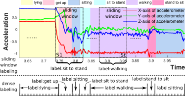
Figure 1: Illustration of different labeling schemes. The top of the figure shows a segment of sensor data collected from a hospitalized patient where different classes of activity are shown in different colors. S1 and St show two example sliding window instances and the predicted labels. The last row shows the predicted labels from dense labeling. The fixed size of the sliding window S1 will cause the loss of label information; it is hard to pre-segment windows dynamically by determining activity boundaries. We can avoid this problem with dense labeling by assigning a label to each sample.

2 Dense Sequence Labeling

Human activity recognition can be viewed as a sequence labeling problem that estimates the class label of activity at each time step in long-term time sequence. The recent human activity recognition methods usually use a sliding window of fixed length to segment the data, and assign a class label to the window base on the label of the last time step (data point) in the window as shown in Fig. 1. However, segmenting a continuous sensor stream is a difficult task, and the exact boundaries of an activity are difficult to define Bulling et al. (2014). As illustrated in Fig. 1, for example, the time series sensor data contains six-class activities. With a fixed sliding window size, one may annotate the class of sliding window $S1$ as sit to stand. However, the window $S1$ contains four-class activities. Class lying, get up, and sitting are lost in window $S1$. Instead of making inaccurate segments that miss activity boundaries, we propose to train and predict the class of every sample densely and without window based labeling as shown in the bottom of Fig. 1. Our method is efficient because we are able to directly generate the dense labels of the sequence in one forward pass of our network without the need for subsampling.

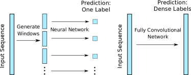
Figure 2: Illustration of prediction procedure of conventional window based approach with CNN (left) and our dense approach with FCN (right). The window based CNN performs one forward pass for predicting one window, and the resulting labels are sub-sampled predictions. In contrast, we only need one forward pass of the network to generate predictions for the entire sequence or a prediction for a single sample (dense labeling).

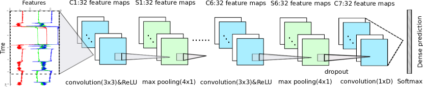
Figure 3: Detailed view of the proposed fully convolutional network architecture. The input 2D time sequence is from the wearable sensors, where one dimension is time and the other is the attributes of all sensors. The proposed model repeats the layers convolution, ReLU, and max pooling six times, where the kernel size is reported in brackets. One dropout layer then performs zeroing operation, followed by the 7-th convolutional layer, where $D$ is the dimension of input data. The final softmax layer performs dense prediction. To ensure the output of each layer is the same length as the input sequence, we add padding in each convolutional and pooling layers.

In the traditional method, generating windows for every time step, which we denote as setting the sampling stride to 1, will also achieve dense predictions of the sequence. However this straight forward and naive approach will result in a huge number of windows and the prediction process will became intractably slow. Specifically, in a conventional CNN based window classification approach, every window requires one forward pass of the CNN network, and it is clearly prohibitively expensive when handling a huge number of windows. This is also the reason that window based methods usually use a large sliding window stride to generate windows to subsample the labels of the original data. Here, we introduce the fully convolutional network (FCN) for this task. We are able to achieve dense and accurate predictions and, at the same time, only require low computational cost for the prediction process; these attributes make our approach an effective solution in practice. Fig. 2 illustrates the different prediction procedure of conventional CNN and the FCN based network. We show the computational performance of the proposed method in Fig. 6.

3 Fully Convolutional Networks for Human Activity Recognition

The main component of the proposed method is a fully convolutional network, which is an extension of convolution neural networks LeCun et al. (1998). CNNs can be viewed as an enhancement of the standard Multi-Layer Perceptron (MLP), where the main difference is the addition of convolutional layers. The basic components in CNN contain convolutional operation, pooling operation, and activation function. When CNNs are constructed by stacking these basic components layer by layer, a network that only contains the nonlinear filter is called Fully Convolutional Network (FCN) Long et al. (2015), which was originally introduced for the task of semantic segmentation. One advantage of FCN is that it can take input of arbitrary size and produce dense prediction with efficient inference and learning. To our best knowledge, we are the first to apply FCN into dense sequence labeling for HAR.

3.1 Network Architecture for Dense Labeling

Here we describe how to exploit FCN architecture for the problem of dense labeling of human activity sequences. The dense labeling estimates the likelihood of a particular activity at a certain time, and then predicts the class of the activity accordingly. The duration—length—of activities vary for different sequences and there are multiple activities in the input sequence, consequently, it is a naturally dense prediction task which requires label prediction for each sample in the sequence. Therefore, it is reasonable to treat the recognition of human activity as a dense labeling problem, where the value at each location points out the confidence of each activity.

The proposed network architecture is shown in Fig. 3. The input to the network is time sequential data and its output is a dense confidence map of the input sequence. We denote the input of layer $l$ at location $(i,j)$ of filter channel $k$ as $\mathbf{x}_{i,j,k}^{l}$, where $1\leq i\leq D^{l}$ is the feature index, $1\leq j\leq T^{l}$ indicates the sample’s location in total $T^{l}$ length sequence, and $1\leq k\leq N_{f}^{l}$ represents the index of filter. The input layer is connected by a convolution layer. For each filter $k$ of layer $l$, the output map is defined as a convolution with a kernel of size $f_{i}^{l}\times f_{j}^{l}$ followed by the addition of a constant “bias” term. To capture local temporal context we restrict each trainable filter with a small size. Let $\mathbf{W}_{i,j,k}^{l}$ be the components of the kernel and $\mathbf{b}_{k}^{l}$ the constant bias for channel $k$ of the layer $l$, respectively. Then the output of a specific location $(i,j)$ in channel $k$ of the layer $l$ is obtained by:

$$\mathbf{z}_{i,j,k}^{l}=\sigma\big{(}\mathbf{b}_{k}^{l}+\sum_{\Delta i=-\bar{f_{i}^{l}}}^{\bar{f_{i}^{l}}}\sum_{\Delta j=\bar{f_{j}^{l}}}^{\bar{f_{j}^{l}}} \sum_{k^{\prime}=1}^{N_{f}^{l}}\mathbf{W}_{\Delta i+\bar{f_{i}^{l}},\Delta j+\bar{f_{j}^{l}},k^{\prime}}^{l}$$

$$\mathbf{x}_{i+\Delta i,j+\Delta j,k^{\prime}}\big{)},$$ (1)

where $\sigma$ is the activation function that introduces the nonlinearity into neural networks and allows it to learn more complex models. In this paper, we use Rectified Linear Units (ReLU) Nair and Hinton (2010) as nonlinearity function in all activation layers. ReLU has been shown to work very well on deep convolutional networks for object recognition, and enforces small amounts of sparsity in neural networks. The ReLU activation function is defined as $\sigma_{ReLU}=\max(0,a)$. The convolution and activation layers are followed by a pooling layer. The purpose of pooling layer is to makes it robust to small variations in previously learned features, which is similar to a smoothing operation. The pooling strategy used in this work is maxpooling, which computes maximum value in each neighborhood at different positions. Recalling the architecture described in Fig. 3, we have kernel size $f_{i}^{l}=3$, $f_{j}^{l}=3$, and the number of filter $N_{f}^{l}=32$ in the first convolutional layer, and $f_{i}^{l}=1$, $f_{j}^{l}=4$, $N_{f}^{l}=32$ in the first pooling layer.

As illustrated in Fig. 3, we repeat those three layers (i.e., convolution, ReLU, and maxpooling), in sequence, six times with the same parameters. Then, the output is passed through a dropout layer that randomly set part of the inputs to zero with a specific probability. Finally, unlike the previous work using CNN architecture, we replace the fully connected layers with convolutional layers. There are $N$ filters in the final convolutional layer, where $N$ is the number of classes of human activities. The kernel size of each filter is $D^{l-1}\times 1$. The last layer of the proposed network is a dense softmax loss layer. Each unit of the output reflects a class membership probability: $p(z=c|\mathbf{x},\mathbf{W},\mathbf{b})=\frac{\exp(\mathbf{W}_{c}\mathbf{x}+\mathbf{b}_{c})}{\sum_{c^{\prime}}\exp(\mathbf{W}_{c^{\prime}}\mathbf{x}+\mathbf{b}_{c^{\prime}})}$. Thus, we can obtain the posterior probability of the dense sequence classification results.

In contrast with the previous CNN methods for human activity recognition Yang et al. (2015); Hammerla et al. (2016); Zeng et al. (2014), we make three important modifications to make the network architecture more suitable for the task of dense labelling of sequences for HAR: i) we replace the fully connected layers with the convolutional layers where the kernel size is $D\times 1$ and stride is $1\times 1$—$D$ is the dimension of input sequence; ii) for our convolution and pooling layers, we use padding to compensate for the kernel size and ensure the output is the same size as the input as shown in Fig. 3, although the number of filters may change; and iii) we apply the dense softmax loss layer which densely impose the softmax classification loss for the predictions of all time steps. This is different from the existing methods which apply the conventional softmax loss layer for the prediction of a single window.

3.2 Efficient Learning and Prediction

The replacement of convolutional layer is very efficient for processing large length time sequences for dense labeling compared with applying sliding windows with the classical CNNs. In computer vision tasks, an FCN is able to classify the whole image at once by considering the summation of loss function of each individual loss at a specific location. However, in human activity recognition problems, we are not able to take the entire long-term time sequence as input to the network. It is computationally and practically prohibitive due to the infinite nature of a time series. In the proposed method, we separate a long-term time sequence into several overlapped subsequences to perform dense prediction. We define subsequence as a partition of length $T$ of contiguous samples from a whole sequence with starting position at $t$. By doing sliding step, we can extract a large amount of overlapped subsequences from a long-term time sequence. Notice that, the proposed subsequence is not the same as sliding window, because we do dense prediction for each sample in a subsequence—i.e.: one label for each sample—instead of predicting the sliding window as a whole—i.e.: one label for all samples. Generally, the length of a subsequence can be far greater than the length of a window. We can define subsequences with sufficiently large length as shown in Fig. 6.

The parameters of the proposed network are trained end-to-end by minimizing the negative log-likelihood function over the training set, summing over all samples in the subsequences:

$$\ell(\mathbf{x},\mathbf{z};\mathbf{W,b})=\sum\nolimits_{j=1}^{T}\ell^{\prime}(\mathbf{x},\mathbf{z}_{j};\mathbf{W,b}),$$ (2)

where $\ell^{\prime}(\mathbf{x},\mathbf{z}_{j};\mathbf{W,b})=-\log\big{(}p(\mathbf{z}_{j}|\mathbf{x},\mathbf{W},\mathbf{b})\big{)}$ represents individual loss of $j$-th sample (data point corresponding to one time step) in a subsequence. The minimization of the loss function is performed by the Stochastic Gradient Descent (SGD) algorithm, where we update the parameters after every subsequence. We compute the gradient over a mini-batch of the training subsequences. We randomly generate a number of subsequences to construct the mini-batch training data.

Once the parameters of the proposed FCN are learned from training data, we use the following two steps to get dense labeling of the whole time sequence. First, the dense confidence maps of each subsequence can be obtained by putting it into the proposed fully convolutional network. Second, because the two adjacent subsequences have overlapped samples, we have to find the overlapped samples and calculate the average probability of being a certain human activity. The final dense prediction (labeling) of time sequence is done by taking the argmax of the average probability of each samples. This prediction scheme is able to classify the whole subsequence at once, which is more efficient than using a sliding window scheme with a stride of one to perform dense labelling.

Table 1: Classification performance of the compared seven methods for locomotion and gesture task of Opportunity dataset on all data, subject 1, subject 2, and subject 3. The highest performance is marked by boldface.

Task	Method	All Data			Subject 1			Subject 2			Subject 3
		$F_{w}$	$NF_{w}$	AC	$F_{w}$	$NF_{w}$	AC	$F_{w}$	$NF_{w}$	AC	$F_{w}$	$NF_{w}$	AC
Locomotion	QDA	76.0	66.3	67.5	80.2	71.3	72.5	75.9	65.7	67.7	77.6	68.0	67.6
	KNN	80.8	80.1	80.3	85.5	85.9	85.9	76.1	77.9	77.5	78.2	73.3	72.7
	SVM	80.7	76.6	77.2	87.1	86.3	86.1	78.5	76.9	77.2	81.8	75.2	75.8
	Baseline	83.6	82.3	82.4	86.6	85.9	86.0	80.3	76.6	76.9	88.5	82.4	83.0
	CNN	83.6	82.6	82.7	87.7	86.7	86.8	85.7	86.0	86.0	88.5	82.1	82.4
	MLP	82.6	79.3	79.7	85.9	84.5	84.4	80.8	79.0	79.1	80.7	73.4	73.8
	Ours	88.7	86.9	87.1	91.9	91.3	91.2	90.1	89.8	89.8	89.0	82.9	83.2
Gesture	QDA	24.5	58.8	50.0	19.3	60.5	52.8	23.7	69.1	62.9	27.1	70.9	67.2
	KNN	45.2	85.2	85.5	45.6	83.6	84.2	46.0	85.5	85.9	49.6	84.1	85.7
	SVM	35.2	82.7	85.0	36.1	82.7	85.8	34.1	82.6	84.8	25.3	77.5	82.3
	Baseline	42.9	84.1	84.4	45.7	84.9	86.4	13.2	78.9	83.2	41.5	82.1	84.4
	CNN	48.8	85.5	85.7	43.4	83.8	84.8	42.1	84.8	86.2	47.6	84.0	86.2
	MLP	39.7	83.1	83.7	47.5	84.9	85.5	42.9	84.9	85.8	28.1	78.3	82.5
	Ours	59.6	89.0	89.9	59.4	89.3	90.5	55.0	88.5	89.7	51.5	85.6	87.4

4 Experiments

We conduct extensive experiments to verify the performance of the proposed dense labeling method for HAR. For FCN, the learning rate for the whole network is set to $10^{-2}$ initially, decreased to $10^{-3}$ after 100 iterations, and training is stopped at 150 iterations. The network weights are learned using the mini-batch (set to 10) SGD algorithm. The length of subsequence is set to 60 for training, and 100 for testing. If there is enough memory, the length of subsequence can be set from 1 to the maximum length of whole test sequence. The adjacent subsequences has 50$\%$ overlap. For sliding window based methods, we set the window size to 24. Experiments were run on a machine with one GPU (NVIDIA GeForce GTX 770), all model are implemented using matlab. We test three non neural network classification techniques (i.e., Quadratic Discriminant Analysis (QDA), K-Nearest Neighbours (KNN, $k=3$) Chavarriaga et al. (2013), and Support Vector Machine (SVM) Chang and Lin (2011)), and three neural network methods (baseline convolution network–Baseline, convolutional neural network based method by Yang et al. (2015)–CNN, and three-layer Multi-Layer Perceptron–MLP). The baseline convolutional network contains four convolution-ReLU-max pooling layers, and follows one fully connected layer and softmax layer. The Baseline, CNN and MPL use a traditional sliding window to generate classifications. The learning rate and iteration parameters of Baseline are set to be the same as ours.

4.1 Dataset

We evaluate the proposed approach on two public benchmark datasets and a new dataset released by our group.

Opportunity dataset. The Opportunity activity recognition dataset Roggen et al. (2010) comprises a set of daily activities collected in a sensor-rich environment. In this paper, we address two kinds of recognition problems: locomotion and gestures, and use the same subset employed in the Opportunity challenge Chavarriaga et al. (2013); Ordóñez and Roggen (2016) to train and test our models. We evaluate the performance on all data, subject 1, subject 2 and subject 3 of the dataset. We use the same training and testing set as in Chavarriaga et al. (2013). Locomotion includes 5 classes with null-class, and gestures contains 18 classes with null-class. Each sample is comprised of 113 real valued attributes, which are scaled to $[0,1]$ for training and prediction; the same data pre-processing method will be applied to the following two datasets.

Hand Gesture dataset. The Hand Gesture dataset Bulling et al. (2014) records arm movements of two people (subject 1 and 2) performing a continuous sequence of different types gestures of daily living. The dataset has 12 classes with null class, and the null class refers to periods with no specific activity. The used data includes three three-axis accelerometers and three two-axis gyroscopes recoding at a sampling rate of 32 Hz. Each sample has 15 real valued sensor attributes in total. For training, testing and validation, we use the same approach as that by Yang et al. (2015) to generate the data.

Table 2: The classification performance of Hand Gesture dataset. The highest performance is marked by boldface.

Method	Subject 1			Subject 2
	$F_{w}$	$NF_{w}$	AC	$F_{w}$	$NF_{w}$	AC
QDA	50.2	46.0	46.7	67.2	63.9	63.1
KNN	85.3	84.5	84.4	85.1	82.9	82.7
SVM	53.6	55.6	57.5	38.0	39.9	45.5
Baseline	77.4	73.0	72.2	80.2	77.4	77.0
CNN	73.7	69.2	68.1	78.9	76.2	75.6
MLP	79.7	80.1	80.1	77.1	75.9	75.5
Ours	89.3	88.2	88.1	88.3	86.1	85.8

Hospital dataset. To verify the performance of the proposed method, we collect our own HAR dataset using an inertial sensor with one accelerometer and one gyroscope. Each sample has 5 real valued attributes in total. We recorded 8 activities from 12 volunteer hospitalised older patients. During the trial, participants were informed only of the types of activities they were required to perform and the inertial sensor was worn loosely over their garments above the sternum area to monitor the activities, which include: lying, stand up (sit to stand), sitting, walking, lie down (get into bed), sit down (stand to sit), get up, and standing. All data is recorded at a frequency of approximately 10 Hz. For all the compared methods, we set the data of the first eight volunteers as training data, the data from the following three volunteers are used for testing, and the last one for validation. This dataset will be publicly available at our project website.

4.2 Evaluation Protocol

Two kinds of evaluation protocols are employed in this paper: classification and misalignment measures.

Classification measures:

We use three widely used metrics: weighted F-measure ($F_{w}$), wighted F-measure with null class ($NF_{w}$), and accuracy (AC). Due to class imbalance in the three datasets, we calculate the F-measure weighted according to their sample proportion: $F_{w}=\sum\nolimits_{i}2\cdot w_{i}\cdot(p_{i}\cdot r_{i})/(p_{i}+r_{i})$ where $i$ is the class index and $w_{i}=n_{i}/N$ with $n_{i}$ the number of samples of the $i$-th class, $N$ the total number of samples and $p_{i}$ denotes precision while $r_{i}$ represents recall. Here $F_{w}$ measures performance without null class.

Table 3: The classification performance of for Hospital dataset. The highest performance is marked by boldface.

	QDA	KNN	SVM	Baseline	CNN	MLP	Ours
$F_{w}$	64.8	79.9	76.2	81.9	81.4	78.4	88.2
AC	70.1	86.6	84.8	88.3	87.0	85.3	91.2

(a)

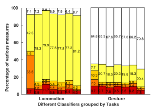
(a) Opportunity Dataset

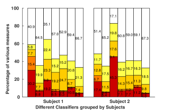
(b) Hand Gesture Dataset

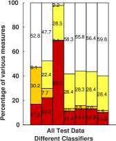
(c) Ours Dataset

Figure 4: Performance evaluation on three datasets for different tasks using the measures proposed by Ward et al. (2011) . Each group of seven columns denotes the accuracy of QDA, KNN, SVM, Baseline, CNN, MLP, and Ours. The digital number on each column shows the exact value of the corresponding measures. Overall our method performs the best.

Misalignment measures:

The classification measures may be misleading when recognizing actions from continuously recorded data. Therefore, we explicitly report different types of errors: True Positive–TP, True Negative–TN, Overfill/Underfill, Insertion, and Fragmentation/Deletion/Substitution Ward et al. (2011) to measure predicted label misalignments with the ground truth. Errors when the start or stop time of a predicted label is earlier or later than the actual time is an Overfill while a predicted label is later or earlier than the actual is an Underfill measure. Predicting an action when there is null activity is an Insertion. Fragmentation denotes the errors of predicting a null class in between an uninterrupted activity class. Deletion represents the errors of assigning a null label when there is an activity. Substitution measures the errors when an activity is misclassified as a different class other than null.

4.3 Results

Comparing the performance of different methods across different studies is difficult for many reasons such as the differing types of experimental protocols and feature used. To make a fair comparison, for QDA, KNN, and SVM methods, we used a sliding window with a fixed step size for extracting the mean value of the sensor on each window as features. The obtained results are quite similar to the benchmark results on the Opportunity dataset Bulling et al. (2014).

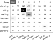
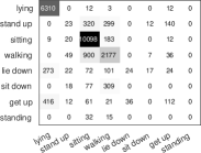
Figure 5: Confusion matrix for Hospital dataset using the proposed method (left) and CNN method (right). Our method is more robust against activity transitions (i.e.: stand up, lie down, sit down, and get up).

We report the classification performance on the three datasets in Tab. 1, Tab. 2 and Tab. 3, respectively. In general, CNN-based methods perform better on almost all dataset than non-CNN methods and our approach, denoted Ours, performs better than all CNN-based methods. Specially, class imbalance leads to overesting the performance of gesture recognition. Ours obtains $59.0\%$ with wighted F-measure on all Opportunity data, which is $11\%$ higher than CNN methods proposed by Yang et al. (2015). A similar conclusion can be drawn in subject 1 and subject 2 for gesture recognition. Those results demonstrate that the proposed dense labeling method is more robust with respect to the class imbalance problem. Note that, we do not report $NF_{w}$ in Tab. 3 because null class is not included in our hospital dataset. Although the proposed approach obtains slight higher accuracy than the baseline method on the new dataset, the $F_{w}$ value of Ours in Tab. 3 is significantly higher than other methods. We advocate that the weighted F-measure can reflect the real performance of unbalanced datasets. Fig. 5 shows the confusion matrix on Hospital dataset generated by our method and CNN method proposed in Yang et al. (2015).

     

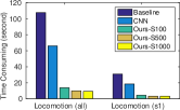
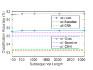
Figure 6: Testing time and accuracy of the compared convolutional networks in CPU-seconds. We can see the testing time (left) and classification accuracy (right) for task locomotion on all and subject 1 (s1) of Opportunity dataset. Ours-S100 denotes the length of the subsequence used for testing our method as being 100. We can see that the performance of our method is insensitive to the length of the subsequence. Unlike traditional CNN based methods that require fixing the sliding window size for testing and training to be identical, a subsequence of our method can be of arbitrary length.

Fig. 4 shows the misalignment performance on the three datasets. For clarity, we only report the overall performance of all Opportunity data in Fig. 4(a), and combine several measures to one term in contrast with the benchmark in Bulling et al. (2014). It can be seen that Ours achieves the best performance among the compared methods. This demonstrates that the dense labeling method more accurately finds the starting and ending point of activities in the temporarily dependent sequence data. Because we do not contain a null class in the Hospital dataset, Fragmentation/Deletion/Substitution term in Fig. 4 (c) only represents the error of Substitution.

We report the computational performance of three convolutional neural networks on Opportunity datasets in Fig. 6. Our approach only consumes one-fifth and one-tenth of the time CNN Yang et al. (2015) and Baseline approach consumed. There are 118,750 and 33,273 samples with 113-D features in all and subject 1 of Opportunity dataset. Note the maximum length of subsequence, 3000, is limited by the machine used for experiments (4GB memory, single GPU).

5 Conclusion

In this paper, we have presented a new, efficient dense labeling approach for human activity recognition using a fully convolutional network. Unlike existing methods, the proposed approach does not rely on a heuristics sliding-window step for producing ambiguous labels of the window—often a source of error during training and prediction. Our approach uses a fully convolutional network framework based on the well-studied deep convolutional neural network theory and therefore making it easy to train and infer the dense labels of sequences as well as benefit from generalization and robustness to extract feature end-to-end. We also release a new dataset publicly for human activity recognition. The promising results demonstrate the effectiveness and efficiency of the proposed dense labeling approach.

References

- Blanke and Schiele [2009] Ulf Blanke and Bernt Schiele. Daily routine recognition through activity spotting. In International Symposium on Location and Context-Awareness, pages 192–206. Springer, 2009.
- Bulling et al. [2012] Andreas Bulling, Jamie A Ward, and Hans Gellersen. Multimodal recognition of reading activity in transit using body-worn sensors. ACM Transactions on Applied Perception, 9(1):2, 2012.
- Bulling et al. [2014] Andreas Bulling, Ulf Blanke, and Bernt Schiele. A tutorial on human activity recognition using body-worn inertial sensors. ACM Computing Surveys (CSUR), 46(3):33, 2014.
- Chang and Lin [2011] Chih-Chung Chang and Chih-Jen Lin. Libsvm: a library for support vector machines. ACM Transactions on Intelligent Systems and Technology (TIST), 2(3):27, 2011.
- Chavarriaga et al. [2013] Ricardo Chavarriaga, Hesam Sagha, Alberto Calatroni, Sundara Tejaswi Digumarti, Gerhard Tröster, José Del R. Millán, and Daniel Roggen. The opportunity challenge: A benchmark database for on-body sensor-based activity recognition. Pattern Recogn. Lett., 34(15):2033–2042, November 2013.
- Hammerla et al. [2016] Nils Y Hammerla, Shane Halloran, and Thomas Ploetz. Deep, convolutional, and recurrent models for human activity recognition using wearables. In International Joint Conference on Artificial Intelligence (IJCAI), pages 1533–1540, 2016.
- Huynh and Schiele [2005] Tâm Huynh and Bernt Schiele. Analyzing features for activity recognition. In Proceedings of the 2005 joint conference on Smart objects and ambient intelligence: innovative context-aware services, pages 159–163. ACM, 2005.
- Krizhevsky et al. [2012] Alex Krizhevsky, Ilya Sutskever, and Geoffrey E Hinton. Imagenet classification with deep convolutional neural networks. In Advances in neural information processing systems, pages 1097–1105, 2012.
- Lane et al. [2015] Nicholas D Lane, Petko Georgiev, and Lorena Qendro. Deepear: robust smartphone audio sensing in unconstrained acoustic environments using deep learning. In Proceedings of the 2015 ACM International Joint Conference on Pervasive and Ubiquitous Computing, pages 283–294. ACM, 2015.
- LeCun et al. [1998] Yann LeCun, Léon Bottou, Yoshua Bengio, and Patrick Haffner. Gradient-based learning applied to document recognition. Proceedings of the IEEE, 86(11):2278–2324, 1998.
- Long et al. [2015] Jonathan Long, Evan Shelhamer, and Trevor Darrell. Fully convolutional networks for semantic segmentation. In Proceedings of the IEEE Conference on Computer Vision and Pattern Recognition, pages 3431–3440, 2015.
- Nair and Hinton [2010] Vinod Nair and Geoffrey E Hinton. Rectified linear units improve restricted boltzmann machines. In Proceedings of the 27th international conference on machine learning (ICML-10), pages 807–814, 2010.
- Neverova et al. [2016] Natalia Neverova, Christian Wolf, Griffin Lacey, Lex Fridman, Deepak Chandra, Brandon Barbello, and Graham Taylor. Learning human identity from motion patterns. IEEE Access, 4:1810–1820, 2016.
- Oliver et al. [2002] Nuria Oliver, Eric Horvitz, and Ashutosh Garg. Layered representations for human activity recognition. In Proceedings of the 4th IEEE International Conference on Multimodal Interfaces, page 3. IEEE Computer Society, 2002.
- Ordóñez and Roggen [2016] Francisco Javier Ordóñez and Daniel Roggen. Deep convolutional and lstm recurrent neural networks for multimodal wearable activity recognition. Sensors, 16(1):115, 2016.
- Plötz et al. [2011] Thomas Plötz, Nils Y Hammerla, and Patrick Olivier. Feature learning for activity recognition in ubiquitous computing. In International Joint Conference on Artificial Intelligence (IJCAI), volume 22, page 1729, 2011.
- Ravi et al. [2005] Nishkam Ravi, Nikhil Dandekar, Preetham Mysore, and Michael L Littman. Activity recognition from accelerometer data. In Aaai, volume 5, pages 1541–1546, 2005.
- Roggen et al. [2010] D. Roggen, A. Calatroni, M. Rossi, T. Holleczek, K. Förster, G. Tröster, P. Lukowicz, D. Bannach, G. Pirkl, A. Ferscha, J. Doppler, C. Holzmann, M. Kurz, G. Holl, R. Chavarriaga, H. Sagha, H. Bayati, M. Creatura, and J. d. R. Millàn. Collecting complex activity datasets in highly rich networked sensor environments. In 2010 Seventh International Conference on Networked Sensing Systems (INSS), pages 233–240, June 2010.
- Shi et al. [2011] Qinfeng Shi, Li Cheng, Li Wang, and Alex Smola. Human action segmentation and recognition using discriminative semi-markov models. International journal of computer vision, 93(1):22–32, 2011.
- Simonyan and Zisserman [2014] Karen Simonyan and Andrew Zisserman. Very deep convolutional networks for large-scale image recognition. arXiv preprint arXiv:1409.1556, 2014.
- Van Kasteren et al. [2008] Tim Van Kasteren, Athanasios Noulas, Gwenn Englebienne, and Ben Kröse. Accurate activity recognition in a home setting. In Proceedings of the 10th international conference on Ubiquitous computing, pages 1–9. ACM, 2008.
- Ward et al. [2011] Jamie A Ward, Paul Lukowicz, and Hans W Gellersen. Performance metrics for activity recognition. ACM Transactions on Intelligent Systems and Technology (TIST), 2(1):6, 2011.
- Yang et al. [2015] Jianbo Yang, Minh Nhut Nguyen, Phyo Phyo San, Xiaoli Li, and Shonali Krishnaswamy. Deep convolutional neural networks on multichannel time series for human activity recognition. In International Joint Conference on Artificial Intelligence (IJCAI), pages 3995–4001, 2015.
- Zeng et al. [2014] Ming Zeng, Le T Nguyen, Bo Yu, Ole J Mengshoel, Jiang Zhu, Pang Wu, and Joy Zhang. Convolutional neural networks for human activity recognition using mobile sensors. In Mobile Computing, Applications and Services, 2014 6th International Conference on, pages 197–205. IEEE, 2014.
- Zhang and Sawchuk [2012] Mi Zhang and Alexander A Sawchuk. Motion primitive-based human activity recognition using a bag-of-features approach. In Proceedings of the 2nd ACM SIGHIT International Health Informatics Symposium, pages 631–640. ACM, 2012.