Implementation of a Distributed Coherent Quantum Observer

Abstract

This paper considers the problem of implementing a previously proposed distributed direct coupling quantum observer for a closed linear quantum system. By modifying the form of the previously proposed observer, the paper proposes a possible experimental implementation of the observer plant system using a non-degenerate parametric amplifier and a chain of optical cavities which are coupled together via optical interconnections. It is shown that the distributed observer converges to a consensus in a time averaged sense in which an output of each element of the observer estimates the specified output of the quantum plant.

I Introduction

In this paper we build on the results of [1] by providing a possible experimental implementation of a direct coupled distributed quantum observer. A number of papers have recently considered the problem of constructing a coherent quantum observer for a quantum system; e.g., see [2, 3, 4]. In the coherent quantum observer problem, a quantum plant is coupled to a quantum observer which is also a quantum system. The quantum observer is constructed to be a physically realizable quantum system so that the system variables of the quantum observer converge in some suitable sense to the system variables of the quantum plant. The papers [5, 6, 1, 7] considered the problem of constructing a direct coupling quantum observer for a given quantum system.

In the papers [4, 2, 5, 1], the quantum plant under consideration is a linear quantum system. In recent years, there has been considerable interest in the modeling and feedback control of linear quantum systems; e.g., see [8, 9, 10]. Such linear quantum systems commonly arise in the area of quantum optics; e.g., see [11, 12]. In addition, the papers [13, 14] have considered the problem of providing a possible experimental implementation of the direct coupled observer described in [5] for the case in which the quantum plant is a single quantum harmonic oscillator and the quantum observer is a single quantum harmonic oscillator. For this case, [13, 14] show that a possible experimental implementation of the augmented quantum plant and quantum observer system may be constructed using a non-degenerate parametric amplifier (NDPA) which is coupled to a beamsplitter by suitable choice of the amplifier and beamsplitter parameters; e.g., see [12] for a description of an NDPA. In this paper, we consider the issue of whether a similar experimental implementation may be provided for the distributed direct coupled quantum observer proposed in [1].

The paper [1] proposes a direct coupled distributed quantum observer which is constructed via the direct connection of many quantum harmonic oscillators in a chain as illustrated in Figure 1. It is shown that this quantum network can be constructed so that each output of the direct coupled distributed quantum observer converges to the plant output of interest in a time averaged sense. This is a form of time averaged quantum consensus for the quantum networks under consideration. However, the experimental implementation approach of [13, 14] cannot be extended in a straightforward way to the direct coupled distributed quantum observer [1]. This is because it is not feasible to extend the NDPA used in [13, 14] to allow for the multiple direct couplings to the multiple observer elements required in the theory of [1]. Hence, in this paper, we modify the theory of [1] to develop a new direct coupled distributed observer in which there is direct coupling only between the plant and the first element of the observer. All of the other couplings between the different elements of the observer are via optical field couplings. This is illustrated in Figure 2. Also, all of the elements of the observer except for the first one are implemented as passive optical cavities. The only active element in the augmented plant observer system is a single NDPA used to implement the plant and first observer element. These features mean that the proposed direct coupling observer is much easier to implement experimentally that the observer which was proposed in [1].

Figure 1: Distributed Quantum Observer of [1].

Figure 2: Distributed Quantum Observer Proposed in This Paper.

We establish that the distributed quantum observer proposed in this paper has very similar properties to the distributed quantum observer proposed in [1] in that each output of the distributed observer converges to the plant output of interest in a time averaged sense. However, an important difference between the observer proposed in [1] and the observer proposed in this paper is that in [1] the output for each observer element corresponded to the same quadrature whereas in this paper, different quadratures are used to define the outputs with a $90^{\circ}$ phase rotation as we move from observer element to element along the chain of observers.

II Quantum Linear Systems

In the distributed quantum observer problem under consideration, both the quantum plant and the distributed quantum observer are linear quantum systems; see also [8, 15, 16]. The quantum mechanical behavior of a linear quantum system is described in terms of the system observables which are self-adjoint operators on an underlying infinite dimensional complex Hilbert space $\mathfrak{H}$. The commutator of two scalar operators $x$ and $y$ on ${\mathfrak{H}}$ is defined as $[x,y]=xy-yx$. Also, for a vector of operators $x$ on ${\mathfrak{H}}$, the commutator of ${x}$ and a scalar operator $y$ on ${\mathfrak{H}}$ is the vector of operators $[{x},y]={x}y-y{x}$, and the commutator of ${x}$ and its adjoint ${x}^{\dagger}$ is the matrix of operators

$$[{x},{x}^{\dagger}]\triangleq{x}{x}^{\dagger}-({x}^{\#}{x}^{T})^{T},$$

where ${x}^{\#}\triangleq(x_{1}^{\ast}\;x_{2}^{\ast}\;\cdots\;x_{n}^{\ast})^{T}$ and ^∗ denotes the operator adjoint.

The dynamics of the closed linear quantum systems under consideration are described by non-commutative differential equations of the form

$$\dot{x}(t) = Ax(t);\quad x(0)=x_{0}$$ (1)

where $A$ is a real matrix in $\mathbb{R}^{n\times n}$, and $x(t)=[\begin{array}[]{ccc}x_{1}(t)&\ldots&x_{n}(t)\end{array}]^{T}$ is a vector of system observables; e.g., see [8]. Here $n$ is assumed to be an even number and $\frac{n}{2}$ is the number of modes in the quantum system.

The initial system variables $x(0)=x_{0}$ are assumed to satisfy the commutation relations

$$[x_{j}(0),x_{k}(0)]=2\imath\Theta_{jk},\ \ j,k=1,\ldots,n,$$ (2)

where $\Theta$ is a real skew-symmetric matrix with components $\Theta_{jk}$. In the case of a single quantum harmonic oscillator, we will choose $x=(x_{1},x_{2})^{T}$ where $x_{1}=q$ is the position operator, and $x_{2}=p$ is the momentum operator. The commutation relations are $[q,p]=2i$. In general, the matrix $\Theta$ is assumed to be of the form

$$\Theta={\rm diag}(J,J,\ldots,J)$$ (3)

where $J$ denotes the real skew-symmetric $2\times 2$ matrix

$$J=\left[\begin{array}[]{cc}0&1\\ -1&0\end{array}\right].$$

The system dynamics (1) are determined by the system Hamiltonian which is a self-adjoint operator on the underlying Hilbert space $\mathfrak{H}$. For the linear quantum systems under consideration, the system Hamiltonian will be a quadratic form $\mathcal{H}=\frac{1}{2}x(0)^{T}Rx(0)$, where $R$ is a real symmetric matrix. Then, the corresponding matrix $A$ in (1) is given by

$$A=2\Theta R.$$ (4)

where $\Theta$ is defined as in (3); e.g., see [8]. In this case, the system variables $x(t)$ will satisfy the commutation relations at all times:

$$[x(t),x(t)^{T}]=2\imath\Theta\ \mbox{for all }t\geq 0.$$ (5)

That is, the system will be physically realizable; e.g., see [8].

Remark 1

Note that that the Hamiltonian $\mathcal{H}$ is preserved in time for the system (1). Indeed, $\mathcal{\dot{H}}=\frac{1}{2}\dot{x}^{T}Rx+\frac{1}{2}x^{T}R\dot{x}=-x^{T}R\Theta Rx+x^{T}R\Theta Rx=0$ since $R$ is symmetric and $\Theta$ is skew-symmetric.

III Direct Coupling Distributed Coherent Quantum Observers

In our proposed direct coupling coherent quantum observer, the quantum plant is a single quantum harmonic oscillator which is a linear quantum system of the form (1) described by the non-commutative differential equation

$$\dot{x}_{p}(t) = A_{p}x_{p}(t);\quad x_{p}(0)=x_{0p};$$

$$z_{p}(t) = C_{p}x_{p}(t)$$ (6)

where $z_{p}(t)$ denotes the vector of system variables to be estimated by the observer and $A_{p}\in\mathbb{R}^{2\times 2}$, $C_{p}\in\mathbb{R}^{1\times 2}$. It is assumed that this quantum plant corresponds to a plant Hamiltonian $\mathcal{H}_{p}=\frac{1}{2}x_{p}(0)^{T}R_{p}x_{p}(0)$. Here $x_{p}=\left[\begin{array}[]{l}q_{p}\\ p_{p}\end{array}\right]$ where $q_{p}$ is the plant position operator and $p_{p}$ is the plant momentum operator. As in [1], in the sequel we will assume that $A_{p}=0$.

We now describe the linear quantum system of the form (1) which will correspond to the distributed quantum observer; see also [8, 15, 16]. This system is described by a non-commutative differential equation of the form

$$\dot{x}_{o}(t) = A_{o}x_{o}(t);\quad x_{o}(0)=x_{0o};$$

$$z_{o}(t) = C_{o}x_{o}(t)$$ (7)

where the observer output $z_{o}(t)$ is the distributed observer estimate vector and $A_{o}\in\mathbb{R}^{n_{o}\times n_{o}}$, $C_{o}\in\mathbb{R}^{\frac{n_{o}}{2}\times n_{o}}$. Also, $x_{o}(t)$ is a vector of self-adjoint non-commutative system variables; e.g., see [8]. We assume the distributed observer order $n_{o}$ is an even number with $N=\frac{n_{o}}{2}$ being the number of elements in the distributed quantum observer. We also assume that the plant variables commute with the observer variables. We will assume that the distributed quantum observer has a chain structure and is coupled to the quantum plant as shown in Figure 2. Furthermore, we write

$$z_{o}=\left[\begin{array}[]{l}z_{o1}\\ z_{o2}\\ \vdots\\ z_{oN}\end{array}\right]$$

where

$$z_{oi}=C_{oi}x_{oi}\mbox{ for }i=1,2,\ldots,N.$$

Note that $C_{oi}\in\mathbb{R}^{1\times 2}$.

The augmented quantum linear system consisting of the quantum plant (6) and the distributed quantum observer (7) is then a quantum system of the form (1) described by equations of the form where

$$\left[\begin{array}[]{l}\dot{x}_{p}(t)\\ \dot{x}_{o1}(t)\\ \dot{x}_{o2}(t)\\ \vdots\\ \dot{x}_{oN}(t)\end{array}\right] = A_{a}\left[\begin{array}[]{l}x_{p}(t)\\ x_{o1}(t)\\ x_{o2}(t)\\ \vdots\\ x_{oN}(t)\end{array}\right];$$ (18)

$$z_{p}(t) = C_{p}x_{p}(t);$$

$$z_{o}(t) = C_{o}x_{o}(t)$$ (19)

where

$$C_{o}=\left[\begin{array}[]{llll}C_{o1}&&&\\ &C_{o2}&0&\\ &0&\ddots&\\ &&&C_{oN}\end{array}\right].$$

We now formally define the notion of a direct coupled linear quantum observer.

Definition 1

The distributed linear quantum observer (7) is said to achieve time-averaged consensus convergence for the quantum plant (6) if the corresponding augmented linear quantum system (19) is such that

$$\lim_{T\rightarrow\infty}\frac{1}{T}\int_{0}^{T}(\left[\begin{array}[]{l}1\\ 1\\ \vdots\\ 1\end{array}\right]z_{p}(t)-z_{o}(t))dt=0.$$ (20)

IV Implementation of a Distributed Quantum Observer

We will consider a distributed quantum observer which has a chain structure and is coupled to the quantum plant as shown in Figure 2. In this distributed quantum observer, there a direct coupling between the quantum plant and the first quantum observer. This direct coupling is determined by a coupling Hamiltonian which defines the coupling between the quantum plant and the first element of the distributed quantum observer:

$$\mathcal{H}_{c}=x_{p}(0)^{T}R_{c}x_{o1}(0).$$ (21)

However, in contrast to [1], there is field coupling between the first quantum observer and all other quantum observers in the chain of observers. The motivation for this structure is that it would be much easier to implement experimentally than the structure proposed in [1]. Indeed, the subsystem consisting of the quantum plant and the first quantum observer can be implemented using an NDPA and a beamsplitter in a similar way to that described in [13, 14]; see also [12] for further details on NDPAs and beamsplitters. This is illustrated in Figure 3.

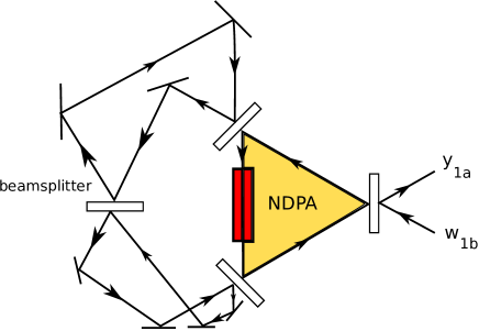
Figure 3: NDPA coupled to a beamsplitter representing the quantum plant and first quantum observer.

Also, the remaining quantum observers in the distributed quantum observer are implemented as simple cavities as shown in Figure 4.

Figure 4: Optical cavity implementation of the remaining quantum observers in the distributed quantum observer.

The proposed quantum optical implementation of a distributed quantum observer is simpler than that of [1]. However, its dynamics are somewhat different than those of the distributed quantum observer proposed in [1]. We now proceed to analyze these dynamics. Indeed, using the results of [14], we can write down quantum stochastic differential equations (QSDEs) describing the plant-first observer system shown in Figure 3:

$$dx_{p} = 2J\alpha\beta^{T}x_{o1}dt;$$

$$dx_{o1} = 2\omega_{1}Jx_{o1}dt-\frac{1}{2}\kappa_{1b}x_{o1}dt+2J\beta\alpha^{T}x_{p}dt$$

$$-\sqrt{\kappa_{1b}}dw_{1b};$$

$$dy_{1a} = \sqrt{\kappa_{1b}}x_{o1}dt+dw_{1b}$$ (22)

where $x_{p}=\left[\begin{array}[]{c}q_{p}\\ p_{p}\end{array}\right]$ is the vector of position and momentum operators for the quantum plant and $x_{o1}=\left[\begin{array}[]{c}q_{1}\\ p_{1}\end{array}\right]$ is the vector of position and momentum operators for the first quantum observer. Here, $\alpha\in\mathbb{R}^{2}$, $\beta\in\mathbb{R}^{2}$ and $\kappa_{1b}>0$ are parameters which depend on the parameters of the beamsplitter and the NDPA. The parameters $\alpha$ and $\beta$ define the coupling Hamiltonian matrix defined in (21) as follows:

$$R_{c}=\alpha\beta^{T}.$$ (23)

In addition, the parameters of the beamsplitter and the NDPA need to be chosen as described in [13, 14] in order to obtain QSDEs of the required form (IV).

The QSDEs describing the $ith$ quantum observer for $i=2,3,\ldots,N-1$ are as follows:

$$dx_{oi} = 2\omega_{i}Jx_{oi}dt-\frac{\kappa_{ia}+\kappa_{ib}}{2}x_{oi}dt$$

$$-\sqrt{\kappa_{ia}}dw_{ia}-\sqrt{\kappa_{ib}}dw_{ib};$$

$$dy_{ia} = \sqrt{\kappa_{ib}}x_{oi}dt+dw_{ib};$$

$$dy_{ib} = \sqrt{\kappa_{ia}}x_{oi}dt+dw_{ia}$$ (24)

where $x_{oi}=\left[\begin{array}[]{c}q_{i}\\ p_{i}\end{array}\right]$ is the vector of position and momentum operators for the $ith$ quantum observer; e.g., see [12]. Here $\kappa_{ia}>0$ and $\kappa_{ib}>0$ are parameters relating to the reflectivity of each of the partially reflecting mirrors which make up the cavity.

The QSDEs describing the $Nth$ quantum observer are as follows:

$$dx_{oN} = 2\omega_{N}Jx_{oN}dt-\frac{\kappa_{Na}}{2}x_{oN}dt-\sqrt{\kappa_{Na}}dw_{Na};$$

$$dy_{Nb} = \sqrt{\kappa_{Na}}x_{oN}dt+dw_{Na}$$ (25)

where $x_{oN}=\left[\begin{array}[]{c}q_{N}\\ p_{N}\end{array}\right]$ is the vector of position and momentum operators for the $Nth$ quantum observer. Here $\kappa_{Na}>0$ is a parameter relating to the reflectivity of the partially reflecting mirror in this cavity.

In addition to the above equations, we also have the following equations which describe the interconnections between the observers as in Figure 2:

$$w_{(i+1)a} = -y_{ia};$$

$$w_{ib} = y_{(i+1)b}$$ (26)

for $i=1,2,\ldots,N-1$.

In order to describe the augmented system consisting of the quantum plant and the quantum observer, we now combine equations (IV), (IV), (IV) and (IV). Indeed, starting with observer $N$, we have from (IV), (IV)

$$dy_{Nb}=\sqrt{\kappa_{Na}}x_{oN}dt-dy_{(N-1)a}.$$

But from (IV) with $i=N-1$,

$$dy_{(N-1)a}=\sqrt{\kappa_{(N-1)b}}x_{o(N-1)}dt+dw_{(N-1)b}.$$

Therefore,

$$dy_{Nb} = \sqrt{\kappa_{Na}}x_{oN}dt-\sqrt{\kappa_{(N-1)b}}x_{o(N-1)}dt-dw_{(N-1)b}$$

$$= \sqrt{\kappa_{Na}}x_{oN}dt-\sqrt{\kappa_{(N-1)b}}x_{o(N-1)}dt-dy_{Nb}$$

using (IV). Hence,

$$dy_{Nb}=\frac{\sqrt{\kappa_{Na}}}{2}x_{oN}dt-\frac{\sqrt{\kappa_{(N-1)b}}}{2}x_{o(N-1)}dt.$$ (27)

From this, it follows using (IV) that

$$dw_{Na} = -\sqrt{\kappa_{Na}}x_{oN}dt+dy_{Nb}$$

$$= -\frac{\sqrt{\kappa_{Na}}}{2}x_{oN}dt-\frac{\sqrt{\kappa_{(N-1)b}}}{2}x_{o(N-1)}dt.$$

Then, using (IV) we obtain the equation

$$dx_{oN}=2\omega_{N}Jx_{oN}dt+\frac{\sqrt{\kappa_{(N-1)b}\kappa_{Na}}}{2}x_{o(N-1)}dt.$$ (28)

We now consider observer $N-1$. Indeed, it follows from (IV) and (IV) with $i=N-1$ that

$$dx_{o(N-1)} = 2\omega_{N-1}Jx_{o(N-1)}dt$$ (29)

$$-\frac{\kappa_{(N-1)a}+\kappa_{(N-1)b}}{2}x_{o(N-1)}dt$$

$$-\sqrt{\kappa_{(N-1)a}}dw_{(N-1)a}-\sqrt{\kappa_{(N-1)b}}dy_{Nb}$$

$$= 2\omega_{N-1}Jx_{o(N-1)}dt$$

$$-\frac{\kappa_{(N-1)a}+\kappa_{(N-1)b}}{2}x_{o(N-1)}dt$$

$$-\sqrt{\kappa_{(N-1)a}}dw_{(N-1)a}$$

$$-\frac{\sqrt{\kappa_{Na}\kappa_{(N-1)b}}}{2}x_{oN}dt$$

$$+\frac{\kappa_{(N-1)b}}{2}x_{o(N-1)}dt$$

$$= 2\omega_{N-1}Jx_{o(N-1)}dt-\frac{\kappa_{(N-1)a}}{2}x_{o(N-1)}dt$$

$$-\frac{\sqrt{\kappa_{Na}\kappa_{(N-1)b}}}{2}x_{oN}dt$$

$$-\sqrt{\kappa_{(N-1)a}}dw_{(N-1)a}$$

using (27). Now using (IV) and (IV) with $i=N-2$, it follows that

$$dy_{(N-2)a} = \sqrt{\kappa_{(N-2)b}}x_{o(N-2)}dt+dw_{(N-2)b}$$

$$= \sqrt{\kappa_{(N-2)b}}x_{o(N-2)}dt+dy_{(N-1)b}$$

$$= \sqrt{\kappa_{(N-2)b}}x_{o(N-2)}dt+\sqrt{\kappa_{(N-1)a}}x_{o(N-1)}dt$$

$$+dw_{(N-1)a}$$

using (IV) with $i=N-1$. Hence using (IV) with $i=N-2$, it follows that

$$dy_{(N-2)a} = \sqrt{\kappa_{(N-2)b}}x_{o(N-2)}dt+\sqrt{\kappa_{(N-1)a}}x_{o(N-1)}dt$$

$$-dy_{(N-2)a}.$$

Therefore

$$dy_{(N-2)a}=\frac{\sqrt{\kappa_{(N-2)b}}}{2}x_{o(N-2)}dt+\frac{\sqrt{\kappa_{(N-1)a}}}{2}x_{o(N-1)}dt.$$

Substituting this into (29), we obtain

$$dx_{o(N-1)} = 2\omega_{N-1}Jx_{o(N-1)}dt$$ (30)

$$-\frac{\sqrt{\kappa_{(N-1)b}\kappa_{Na}}}{2}x_{oN}dt$$

$$+\frac{\sqrt{\kappa_{(N-2)b}\kappa_{(N-1)a}}}{2}x_{o(N-2)}dt.$$

Continuing this process, we obtain the following QSDEs for the variables $x_{oi}$:

$$dx_{oi} = 2\omega_{i}Jx_{oi}dt$$ (31)

$$-\frac{\sqrt{\kappa_{ib}\kappa_{(i+1)a}}}{2}x_{o(i+1)}dt$$

$$+\frac{\sqrt{\kappa_{(i-1)b}\kappa_{ia}}}{2}x_{o(i-1)}dt$$

for $i=2,3,\ldots,N-1$. Finally for $x_{o1}$, we obtain

$$dx_{o1} = 2\omega_{1}Jx_{o1}dt-\frac{\sqrt{\kappa_{1b}\kappa_{(2a}}}{2}x_{o2}dt\ +2J\beta\alpha^{T}x_{p}dt.$$

We now observe that the plant equation

$$dx_{p} = 2J\alpha\beta^{T}x_{o1}dt$$

implies that the quantity

$$z_{p}=\alpha^{T}x_{p}$$

satisfies

$$dz_{p}=2\alpha^{T}J\alpha\beta^{T}x_{o1}dt=0$$

since $J$ is a skew-symmetric matrix. Therefore,

$$z_{p}(t)=z_{p}(0)=z_{p}$$ (34)

for all $t\geq 0$.

We now combine equations (IV), (31), (28) and write them in vector-matrix form. Indeed, let

$$x_{o}=\left[\begin{array}[]{c}x_{o1}\\ x_{o2}\\ \vdots\\ x_{oN}\end{array}\right].$$

Then, we can write

$$\dot{x}_{o}=A_{o}x_{o}+B_{o}z_{p}$$

where

$$A_{o}=$$ (41)

$$2\left[\begin{array}[]{rrrrrr}\omega_{1}J&-\mu_{2}I&&&&\\ \mu_{2}I&\omega_{2}J&-\mu_{3}I&&0&\\ &\mu_{3}I&\omega_{3}J&-\mu_{4}I&&\\ &&\ddots&\ddots&\ddots&\\ 0&&&\mu_{N-1}I&\omega_{N-1}J&-\mu_{N}I\\ &&&&\mu_{N}I&\omega_{N}J\end{array}\right],$$

$$B_{o}=$$ (46)

$$2\left[\begin{array}[]{r}J\beta\\ 0\\ \vdots\\ 0\end{array}\right]$$

and

$$\mu_{i}=\frac{1}{4}\sqrt{\kappa_{(i-1)b}\kappa_{ia}}>0$$

for $i=2,3,\ldots,N$.

To construct a suitable distributed quantum observer, we will further assume that

$$\beta = -\mu_{1}\alpha,$$

$$C_{p} = \alpha^{T},$$ (47)

where $\mu_{1}>0$ and

$$C_{o}=$$ (54)

$$\frac{1}{\|\alpha\|^{2}}\left[\begin{array}[]{llllll}\alpha^{T}&&&&&\\ &-J\alpha^{T}&&&0&\\ &&-\alpha^{T}&&&\\ &&&J\alpha^{T}&&\\ &0&&&\ddots&\\ &&&&&(-J)^{N-1}\alpha^{T}\end{array}\right].$$

This choice of the matrix $C_{o}$ means that different quadratures are used for the outputs of the elements of the distributed quantum observer with a $90^{\circ}$ phase rotation as we move from observer element to element along the chain of observers.

In order to construct suitable values for the quantities $\mu_{i}$ and $\omega_{i}$, we require that

$$A_{o}\bar{x}_{o}+B_{o}z_{p}=0$$ (56)

where

$$\bar{x}_{o}=\left[\begin{array}[]{c}\alpha\\ J\alpha\\ -\alpha\\ -J\alpha\\ \alpha\\ \vdots\\ (J)^{N-1}\alpha\end{array}\right]z_{p}.$$

This will ensure that the quantity

$$x_{e}=x_{o}-\bar{x}_{o}$$ (57)

will satisfy the non-commutative differential equation

$$\dot{x}_{e}=A_{o}x_{e}.$$ (58)

This, combined with the fact that

$$C_{o}\bar{x}_{o} = \frac{1}{\|\alpha\|^{2}}\left[\begin{array}[]{llll}\alpha^{T}&&&\\ &-J\alpha^{T}&0&\\ &0&\ddots&\\ &&&(-J)^{N-1}\alpha^{T}\end{array}\right]$$ (68)

$$\times\left[\begin{array}[]{l}\alpha\\ J\alpha\\ \vdots\\ (J)^{N-1}\alpha\end{array}\right]z_{p}$$

$$= \left[\begin{array}[]{l}1\\ 1\\ \vdots\\ 1\end{array}\right]z_{p}$$ (73)

will be used in establishing condition (20) for the distributed quantum observer.

Now, we require

$$A_{o}\left[\begin{array}[]{c}\alpha\\ J\alpha\\ -\alpha\\ -J\alpha\\ \alpha\\ \vdots\\ (J)^{N-1}\end{array}\right]+B_{o}$$

$$= 2\left[\begin{array}[]{c}\omega_{1}J\alpha-\mu_{2}J\alpha-\mu_{1}J\alpha\\ \mu_{2}\alpha-\omega_{2}\alpha+\mu_{3}\alpha\\ \mu_{3}J\alpha-\omega_{3}J\alpha+\mu_{4}J\alpha\\ \vdots\\ \mu_{N}(J)^{N-2}\alpha+\omega_{N}J^{N}\alpha\end{array}\right]$$

$$= 0.$$

This will be satisfied if and only if

$$\left[\begin{array}[]{c}\omega_{1}-\mu_{2}-\mu_{1}\\ \mu_{2}-\omega_{2}+\mu_{3}\\ \mu_{3}-\omega_{3}+\mu_{4}\\ \vdots\\ \mu_{N}-\omega_{N}\end{array}\right]=0.$$

That is, we will assume that

$$\omega_{i}=\mu_{i}+\mu_{i+1}$$ (76)

for $i=1,2,\ldots,N-1$ and

$$\omega_{N}=\mu_{N}.$$ (77)

To show that the above candidate distributed quantum observer leads to the satisfaction of the condition (20), we first note that $x_{e}$ defined in (57) will satisfy (58). If we can show that

$$\lim_{T\rightarrow\infty}\frac{1}{T}\int_{0}^{T}x_{e}(t)dt=0,$$ (78)

then it will follow from (68) and (57) that (20) is satisfied. In order to establish (78), we first note that we can write

$$A_{o}=2\Theta R_{o}$$

where

$$R_{o}=$$

$$\left[\begin{array}[]{rrrrrr}\omega_{1}I&\mu_{2}J&&&&\\ -\mu_{2}J&\omega_{2}I&\mu_{3}J&&0&\\ &-\mu_{3}J&\omega_{3}I&\mu_{4}J&&\\ &&\ddots&\ddots&\ddots&\\ &0&&-\mu_{N-1}J&\omega_{N-1}I&\mu_{N}J\\ &&&&-\mu_{N}J&\omega_{N}I\end{array}\right].$$

We will now show that the symmetric matrix $R_{o}$ is positive-definite.

Lemma 1

The matrix $R_{o}$ is positive definite.

Proof:

In order to establish this lemma, let

$$x_{o}=\left[\begin{array}[]{l}x_{o1}\\ x_{o2}\\ \vdots\\ x_{oN}\end{array}\right]\in\mathbb{R}^{2N}$$

where $x_{oi}=\left[\begin{array}[]{c}q_{i}\\ p_{i}\end{array}\right]\in\mathbb{R}^{2}$ for $i=1,2,\ldots,N$. Also, define the complex scalars $a_{i}=q_{i}+\imath p_{i}$ for $i=1,2,\ldots,N$. Then it is straightforward to verify that

$$x_{o}^{T}R_{o}x_{o} = \omega_{1}\|x_{o1}\|^{2}-2\mu_{2}x_{o1}^{T}\alpha x_{o2}^{T}\alpha+\omega_{2}\|x_{o2}\|^{2}$$

$$-2\mu_{3}x_{o2}^{T}\alpha x_{o3}^{T}\alpha+\omega_{3}\|x_{o3}\|^{2}$$

$$\vdots$$

$$-2\mu_{N}x_{oN-1}^{T}\alpha x_{oN}^{T}\alpha+\omega_{N}\|x_{oN}\|^{2}$$

$$= \omega_{1}a_{1}^{*}a_{1}-\imath\mu_{2}a_{1}^{*}a_{2}+\imath\mu_{2}a_{2}^{*}a_{1}+\omega_{2}a_{2}^{*}a_{2}$$

$$-\imath\mu_{3}a_{2}^{*}a_{3}+\imath\mu_{3}a_{3}^{*}a_{2}+\omega_{3}a_{3}^{*}a_{3}$$

$$\vdots$$

$$-\imath\mu_{N}a_{N-1}^{*}a_{N}+\imath\mu_{N}a_{N}^{*}a_{N-1}+\omega_{N}a_{N}^{*}a_{N}$$

$$= a_{o}^{\dagger}\tilde{R}_{o}a_{o}$$

where

$$a_{o}=\left[\begin{array}[]{l}a_{1}\\ a_{2}\\ \vdots\\ a_{N}\end{array}\right]\in\mathbb{C}^{N}$$

and

$$\tilde{R}_{o}=\left[\begin{array}[]{rrrrr}\omega_{1}&-\imath\mu_{2}&&&\\ \imath\mu_{2}&\omega_{2}&-\imath\mu_{3}&&0\\ &\imath\mu_{3}&\omega_{3}&\ddots&\\ 0&&\ddots&\ddots&-\imath\mu_{N}\\ &&&\imath\mu_{N}&\omega_{N}\end{array}\right].$$

Here ^† denotes the complex conjugate transpose of a vector. From this, it follows that the real symmetric matrix $R_{o}$ is positive-definite if and only if the complex Hermitian matrix $\tilde{R}_{o}$ is positive-definite.

To prove that $\tilde{R}_{o}$ is positive-definite, we first substitute the equations (76) and (77) into the definition of $\tilde{R}_{o}$ to obtain

$$\tilde{R}_{o} = \left[\begin{array}[]{rrrrr}\mu_{1}+\mu_{2}&-\imath\mu_{2}&&&\\ \imath\mu_{2}&\mu_{2}+\mu_{3}&-\imath\mu_{3}&&0\\ &\imath\mu_{3}&\mu_{3}+\mu_{4}&\ddots&\\ 0&&\ddots&\ddots&-\imath\mu_{N}\\ &&&\imath\mu_{N}&\mu_{N}\end{array}\right]$$

$$= \tilde{R}_{o1}+\tilde{R}_{o2}$$

where

$$\tilde{R}_{o1}=\left[\begin{array}[]{rrrr}\mu_{1}&0&\ldots&0\\ 0&0&\ldots&0\\ \vdots&&&\vdots\\ 0&0&\ldots&0\end{array}\right]\geq 0$$

and

$$\tilde{R}_{o2}=\left[\begin{array}[]{rrrrr}\mu_{2}&-\imath\mu_{2}&&&\\ +\imath\mu_{2}&\mu_{2}+\mu_{3}&-\imath\mu_{3}&&0\\ &+\imath\mu_{3}&\mu_{3}+\mu_{4}&\ddots&\\ 0&&\ddots&\ddots&-\imath\mu_{N}\\ &&&+\imath\mu_{N}&\mu_{N}\end{array}\right].$$

Now, we can write

$$a_{o}^{\dagger}\tilde{R}_{o2}a_{o} = \mu_{2}a_{1}^{*}a_{1}-\imath\mu_{2}a_{1}^{*}a_{2}+\imath\mu_{2}a_{2}^{*}a_{1}+\mu_{2}a_{2}^{*}a_{2}$$

$$+\mu_{3}a_{2}^{*}a_{2}-\imath\mu_{3}a_{2}^{*}a_{3}+\imath\mu_{3}a_{3}^{*}a_{2}+\mu_{4}a_{3}^{*}a_{3}$$

$$\vdots$$

$$+\mu_{N-1}a_{N-1}^{*}a_{N-1}-\imath\mu_{N}a_{N-1}^{*}a_{N}$$

$$+\imath\mu_{N}a_{N}^{*}a_{N-1}+\mu_{N}a_{N}^{*}a_{N}$$

$$= \mu_{2}(-\imath a_{1}^{*}+a_{2}^{*})(\imath a_{1}+a_{2})$$

$$+\mu_{3}(-\imath a_{2}^{*}+a_{3}^{*})(\imath a_{2}+a_{3})$$

$$\vdots$$

$$+\mu_{N}(-\imath a_{N-1}^{*}+a_{N}^{*})(\imath a_{N-1}+a_{N})$$

$$\geq 0.$$

Thus, $\tilde{R}_{o2}\geq 0$. Furthermore, $a_{o}^{\dagger}\tilde{R}_{o2}a_{o}=0$ if and only if

$$a_{2} = -\imath a_{1};$$

$$a_{3} = -\imath a_{2};$$

$$\vdots$$

$$a_{N} = -\imath a_{N-1}.$$

That is, the null space of $\tilde{R}_{o2}$ is given by

$$\mathcal{N}(\tilde{R}_{o2})=\mbox{span}\{\left[\begin{array}[]{l}1\\ -\imath\\ -1\\ \imath\\ 1\\ \vdots\\ (-\imath)^{N-1}\end{array}\right]\}.$$

The fact that $\tilde{R}_{o1}\geq 0$ and $\tilde{R}_{o2}\geq 0$ implies that $\tilde{R}_{o}\geq 0$. In order to show that $\tilde{R}_{o}>0$, suppose that $a_{o}$ is a non-zero vector in $\mathcal{N}(\tilde{R}_{o})$. It follows that

$$a_{o}^{\dagger}\tilde{R}_{o}a_{o}=a_{o}^{\dagger}\tilde{R}_{o1}a_{o}+a_{o}^{\dagger}\tilde{R}_{o2}a_{o}=0.$$

Since $\tilde{R}_{o1}\geq 0$ and $\tilde{R}_{o2}\geq 0$, $a_{o}$ must be contained in the null space of $\tilde{R}_{o1}$ and the null space of $\tilde{R}_{o2}$. Therefore $a_{o}$ must be of the form

$$a_{o}=\gamma\left[\begin{array}[]{l}1\\ -\imath\\ -1\\ \imath\\ 1\\ \vdots\\ (-\imath)^{N-1}\end{array}\right]$$

where $\gamma\neq 0$. However, then

$$a_{o}^{\dagger}\tilde{R}_{o1}a_{o}=\gamma^{2}\tilde{\mu}_{1}\neq 0$$

and hence $a_{o}$ cannot be in the null space of $\tilde{R}_{o1}$. Thus, we can conclude that the matrix $\tilde{R}_{o}$ is positive definite and hence, the matrix $R_{o}$ is positive definite. This completes the proof of the lemma. ∎

We now verify that the condition (20) is satisfied for the distributed quantum observer under consideration. This proof follows along very similar lines to the corresponding proof given in [1]. We recall from Remark 1 that the quantity $\frac{1}{2}x_{e}(t)^{T}R_{o}x_{e}(t)$ remains constant in time for the linear system:

$$\dot{x}_{e}=A_{o}x_{e}=2\Theta R_{o}x_{e}.$$

That is

$$\frac{1}{2}x_{e}(t)^{T}R_{o}x_{e}(t)=\frac{1}{2}x_{e}(0)^{T}R_{o}x_{e}(0)\quad\forall t\geq 0.$$ (81)

However, $x_{e}(t)=e^{2\Theta R_{o}t}x_{e}(0)$ and $R_{o}>0$. Therefore, it follows from (81) that

$$\sqrt{\lambda_{min}(R_{o})}\|e^{2\Theta R_{o}t}x_{e}(0)\|\leq\sqrt{\lambda_{max}(R_{o})}\|x_{e}(0)\|$$

for all $x_{e}(0)$ and $t\geq 0$. Hence,

$$\|e^{2\Theta R_{o}t}\|\leq\sqrt{\frac{\lambda_{max}(R_{o})}{\lambda_{min}(R_{o})}}$$ (82)

for all $t\geq 0$.

Now since $\Theta$ and $R_{o}$ are non-singular,

$$\int_{0}^{T}e^{2\Theta R_{o}t}dt=\frac{1}{2}e^{2\Theta R_{o}T}R_{o}^{-1}\Theta^{-1}-\frac{1}{2}R_{o}^{-1}\Theta^{-1}$$

and therefore, it follows from (82) that

$$\frac{1}{T}\|\int_{0}^{T}e^{2\Theta R_{o}t}dt\|$$

$$= \frac{1}{T}\|\frac{1}{2}e^{2\Theta R_{o}T}R_{o}^{-1}\Theta^{-1}-\frac{1}{2}R_{o}^{-1}\Theta^{-1}\|$$

$$\leq \frac{1}{2T}\|e^{2\Theta R_{o}T}\|\|R_{o}^{-1}\Theta^{-1}\|$$

$$+\frac{1}{2T}\|R_{o}^{-1}\Theta^{-1}\|$$

$$\leq \frac{1}{2T}\sqrt{\frac{\lambda_{max}(R_{o})}{\lambda_{min}(R_{o})}}\|R_{o}^{-1}\Theta^{-1}\|$$

$$+\frac{1}{2T}\|R_{o}^{-1}\Theta^{-1}\|$$

$$\rightarrow 0$$

as $T\rightarrow\infty$. Hence,

$$\lim_{T\rightarrow\infty}\frac{1}{T}\|\int_{0}^{T}x_{e}(t)dt\|$$

$$= \lim_{T\rightarrow\infty}\frac{1}{T}\|\int_{0}^{T}e^{2\Theta R_{o}t}x_{e}(0)dt\|$$

$$\leq \lim_{T\rightarrow\infty}\frac{1}{T}\|\int_{0}^{T}e^{2\Theta R_{o}t}dt\|\|x_{e}(0)\|$$

$$= 0.$$

This implies

$$\lim_{T\rightarrow\infty}\frac{1}{T}\int_{0}^{T}x_{e}(t)dt=0$$

and hence, it follows from (57) and (68) that

$$\lim_{T\rightarrow\infty}\frac{1}{T}\int_{0}^{T}z_{o}(t)dt=\left[\begin{array}[]{l}1\\ 1\\ \vdots\\ 1\end{array}\right]z_{p}.$$

Also, (34) implies

$$\lim_{T\rightarrow\infty}\frac{1}{T}\int_{0}^{T}z_{p}(t)dt=\left[\begin{array}[]{l}1\\ 1\\ \vdots\\ 1\end{array}\right]z_{p}.$$

Therefore, condition (20) is satisfied. Thus, we have established the following theorem.

Theorem 1

Consider a quantum plant of the form (6) where $A_{p}=0$. Then the distributed direct coupled quantum observer defined by equations (7), (21), (23), (41), (IV), (54), (76), (77) achieves time-averaged consensus convergence for this quantum plant.

References

• [1] I. R. Petersen, “Time averaged consensus in a direct coupled distributed coherent quantum observer,” in Proceedings of the 2015 American Control Conference, Chicago, IL, July 2015.
• [2] I. Vladimirov and I. R. Petersen, “Coherent quantum filtering for physically realizable linear quantum plants,” in Proceedings of the 2013 European Control Conference, Zurich, Switzerland, July 2013.
• [3] Z. Miao, L. A. D. Espinosa, I. R. Petersen, V. Ugrinovskii, and M. R. James, “Coherent quantum observers for n-level quantum systems,” in Australian Control Conference, Perth, Australia, November 2013.
• [4] Z. Miao, M. R. James, and I. R. Petersen, “Coherent observers for linear quantum stochastic systems,” Automatica, vol. 71, pp. 264–271, 2016.
• [5] I. R. Petersen, “A direct coupling coherent quantum observer,” in Proceedings of the 2014 IEEE Multi-conference on Systems and Control, Antibes, France, October 2014, also available arXiv 1408.0399.
• [6] ——, “A direct coupling coherent quantum observer for a single qubit finite level quantum system,” in Proceedings of 2014 Australian Control Conference, Canberra, Australia, November 2014, also arXiv 1409.2594.
• [7] ——, “Time averaged consensus in a direct coupled coherent quantum observer network for a single qubit finite level quantum system,” in Proceedings of the 10th ASIAN CONTROL CONFERENCE 2015, Kota Kinabalu, Malaysia, May 2015.
• [8] M. R. James, H. I. Nurdin, and I. R. Petersen, “${H}^{\infty}$ control of linear quantum stochastic systems,” IEEE Transactions on Automatic Control, vol. 53, no. 8, pp. 1787–1803, 2008.
• [9] H. I. Nurdin, M. R. James, and I. R. Petersen, “Coherent quantum LQG control,” Automatica, vol. 45, no. 8, pp. 1837–1846, 2009.
• [10] A. J. Shaiju and I. R. Petersen, “A frequency domain condition for the physical realizability of linear quantum systems,” IEEE Transactions on Automatic Control, vol. 57, no. 8, pp. 2033 – 2044, 2012.
• [11] C. Gardiner and P. Zoller, Quantum Noise.   Berlin: Springer, 2000.
• [12] H. Bachor and T. Ralph, A Guide to Experiments in Quantum Optics, 2nd ed.   Weinheim, Germany: Wiley-VCH, 2004.
• [13] I. R. Petersen and E. H. Huntington, “A possible implementation of a direct coupling coherent quantum observer,” in Proceedings of 2015 Australian Control Conference, Gold Coast, Australia, November 2015.
• [14] I. R. Petersen and E. Huntington, “Implementation of a direct coupling coherent quantum observer including observer measurements,” in Proceedings of the 2016 American Control Conference, Boston, MA, July 2016.
• [15] J. Gough and M. R. James, “The series product and its application to quantum feedforward and feedback networks,” IEEE Transactions on Automatic Control, vol. 54, no. 11, pp. 2530–2544, 2009.
• [16] G. Zhang and M. James, “Direct and indirect couplings in coherent feedback control of linear quantum systems,” IEEE Transactions on Automatic Control, vol. 56, no. 7, pp. 1535–1550, 2011.