Just DIAL: DomaIn Alignment Layers for Unsupervised Domain Adaptation

Abstract

The empirical fact that classifiers, trained on given data collections, perform poorly when tested on data acquired in different settings is theoretically explained in domain adaptation through a shift among distributions of the source and target domains. Alleviating the domain shift problem, especially in the challenging setting where no labeled data are available for the target domain, is paramount for having visual recognition systems working in the wild. As the problem stems from a shift among distributions, intuitively one should try to align them. In the literature, this has resulted in a stream of works attempting to align the feature representations learned from the source and target domains by introducing appropriate regularization terms in the objective function. In this work we propose a different strategy and we act directly at the distribution level by introducing DomaIn Alignment Layers (DIAL) which reduce the domain shift by matching the source and target feature distributions to a canonical one. Our experimental evaluation, conducted on a widely used public benchmark, demonstrates the advantages of the proposed domain adaptation strategy.

1 Introduction

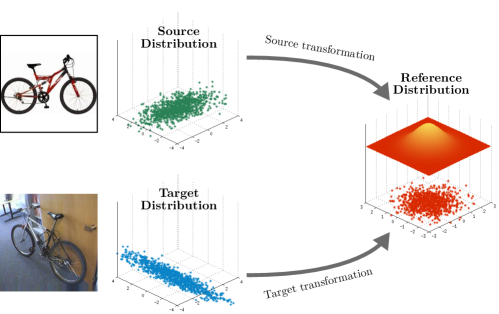
Figure 1: DIAL learn a pair of transformations that shift the observed source and target distribution to match a desired reference distribution.

Many scientists today believe we are witnessing the golden age of computer vision. The massive adoption of machine learning and, in particular, of deep learning techniques as well as the availability of large fully annotated datasets have enabled amazing progresses in the field. A natural question is if the novel generation of computer vision technologies is robust enough to operate in real world scenarios. One of the fundamental requirements for developing systems working in the wild is devising computational models which are immune to the domain shift problem, i.e. which are accurate when test data are drawn from a (slightly) different data distribution than training samples. Unfortunately, recent studies in the literature have shown that, even with powerful deep architectures, the domain shift problem can only be alleviated but not entirely solved [1] and several methods for deep domain adaptation have been developed.

Domain adaptation focuses on learning classification or regression models on some target data by exploiting additional knowledge derived from a related source task. In particular, unsupervised domain adaptation focuses on the challenging scenario where no labeled data are available in the target domain. Several approaches have been proposed for unsupervised domain adaptation in the past, the most successful of which are based on deep architectures [2, 3, 4, 5]. Previous unsupervised domain adaptation methods can be roughly divided in two categories. The first category includes methods which attempt to reduce the discrepancy between source and target distributions by minimizing the distance between the mean embeddings of the learned representations, i.e. the so-called Maximum Mean Discrepancy (MMD) [2, 5]. A second class of methods learns domain invariant features by maximizing a domain-confusion objective function, modelling the loss of an auxiliary classifier which should discriminate if a sample belongs to the source or to the target domain [3, 4].

Following these recent approaches, in this paper we present a domain adaptation method which simultaneously learns discriminative deep representations while coping with domain shift in the unsupervised setting. Differently from previous works, we do not focus on learning domain-invariant features by explicitly optimizing additional loss terms (e.g. MMD, domain-confusion). We argue instead that domain adaptation can be achieved by embedding in the network some Domain Alignment layers (DA-layers) which operate by aligning both source and target distributions to a canonical one. We also show that several different transformations can be employed in our DA-layers to match source and target data distributions to the reference, thus highlighting the generality of our approach. We call our algorithm DIAL – DomaIn Alignment Layers. Our experimental evaluation, conducted on the most widely used domain adaptation benchmark, i.e. the Office-31 [6] dataset, demonstrates that DIAL greatly alleviates the domain discrepancy and outperforms most state of the art techniques.

2 Related Work

In the last decade unsupervised domain adaptation have received considerable interest in the computer vision community as in many applications labeled data are not available in the target domain [7, 8, 9, 10, 11, 12, 13, 2, 3, 4].

Traditional methods for unsupervised domain adaptation attempt to reduce the domain shift by adopting two main approaches. A first strategy, the so-called instance re-weighting [7, 8, 9, 10, 11], is based on building models for the target domain by adopting appropriately re-weighted source samples. The idea is to assign different importance to source samples such as to reflect their similarity with the target data. This approach has been proposed in [7] where a nonparametric method called Kernel Mean Matching is used to set weights without explicitly estimating the data distributions. Similarly, Gong et al. [10] introduced the notion of landmark datapoints, a subset of source samples which are similar to target data, and proposed a landmark-based domain adaptation method. Chu et al. [8] presented a framework for joint source sample selection and classifier learning. While these works considered hand-crafted features, similar ideas can be also exploited in the case of deep architectures. An example is the work in [11] where deep autoencoders are used to build source sample weights.

The large majority of previous unsupervised domain adaptation methods are based on feature alignment, i.e. domain shift is reduced by projecting source and target data in a common subspace. Several feature alignment methods have been proposed in the past, both considering shallow models [14, 15, 16] and deep architectures [2, 3, 4]. Focusing on works adopting deep architectures, most methods align source and target feature representations by adding in the objective function a regularization term attempting to (i) reduce Maximum Mean Discrepancy [2, 5, 17] or (ii) maximize a domain confusion loss [3, 4]. Recent studies have also investigated alternative methodologies, such as building specific encoder-decoder networks to jointly learn source labels and reconstruct unsupervised target images  [18, 19]. Our approach significantly departs from previous works by reducing the discrepancy between source and target distributions through the introduction of our DA-layers. The most similar work to ours is [20] where Li et al. proposed to revisit batch normalization for deep domain adaptation. While our approach develops from a similar intuition, our method can be regarded as a generalization of [20], as we consider several transformation in our DA layers and we introduce a prior over the network parameters in order to benefit from the target samples during training. Experiments presented in Sec. 4 show the significant added value of our idea.

3 DIAL: DomaIn Alignment Layers

Let $\mathcal{X}$ and $\mathcal{Y}$ denote the input space (e.g. images) and the output space (e.g. image categories) of our learning task, respectively. We consider an unsupervised domain adaptation setting, where we have a source domain described in terms of a probability distribution $p^{s}_{\mathtt{x}y}$ over $\mathcal{X}\times\mathcal{Y}$ and a target domain following $p^{t}_{\mathtt{x}y}$. The source and target distributions differ in general and are unknown, but we are provided with $n$ labeled observations $\mathcal{S}=\{(x_{1}^{s},y_{1}^{s}),\ldots,(x_{n}^{s},y_{n}^{s})\}$ from the source domain, i.e. they are sampled from $p^{s}_{\mathtt{x}y}$, and $m$ unlabeled observations $\mathcal{T}=\{x_{1}^{t},\ldots,x_{m}^{t}\}$ sampled from the marginal distribution $p^{t}_{\mathtt{x}}$. The goal of the learning task is to estimate a predictor for the target domain, using the observations in $\mathcal{S}$ and $\mathcal{T}$. This task is particularly challenging because we lack observed labels from the target domain and the discrepancy between the source and target domains, which in general exists, prevents predictors trained on the source domain to be readily applicable to samples from the target domain.

One key element for the success of an unsupervised domain adaptation algorithm is its ability of reducing the discrepancy between source and target domains. There are different approaches to achieve this goal, but we focus on aligning the domains at the feature level. Within this family of methods the most successful ones couple the training process and the domain adaptation step within deep neural architectures [4, 5, 2], yielding alignments at different level of abstractions. Our method is close in spirit to this line of works but we distinguish from them by (a) not relying on the covariate shift assumption, i.e. we in general assume $p^{s}_{\mathtt{y}|x}\neq p^{t}_{\mathtt{y}|x}$, and by (b) hard-coding the domain-invariance properties directly into our deep neural network. The rationale behind the former choice is the impossibility theorem for domain adaptation given in [21], which intuitively states that no domain adaptation algorithm can succeed (in terms of the notion of learnability) if it relies on the covariate shift assumption and achieves a low discrepancy between the source and target unlabeled distributions, i.e. $p^{s}_{\mathtt{x}}$ and $p^{t}_{\mathtt{x}}$, respectively. Since the latter assumption is what one implicitly pursues by performing domain alignments at the feature level, we drop the former assumption. The other distinguishing aspect of our method is an architectural solution to achieve domain-invariance, which contrasts with the majority of approaches that rely on additional loss terms (e.g. MMD-type losses [2] or adversarial losses [3, 4]) that induce an external pressure on the networks’ parameters at training time to fulfill the domain-invariance requirement. Works exists that do not rely on the covariate-shift assumption and take a loss-based approach to feature alignment, but those typically implement the source and target predictors using different sets of parameters (not necessarily disjoint) [22, 5]. Instead, the method we propose is able to avoid the covariate shift assumption and at the same time have the set of learnable network parameters, denoted by $\theta$ in this work, that is totally shared. The key element of our method is the domain-alignment layer that we describe below.

3.1 Source and Target Predictors

We implement source and target predictors as two deep neural networks that share the same structure and the same parameters given by $\theta$. However, the two networks differ by having a number of layers that perform a domain-specific operation. Those layers are called Domain-Alignment Layers (DA-layers) and their role is to apply a data transformation that aligns the input distribution to a pre-fixed reference distribution. In Figure 1, we provide an illustration of the basic principle. In general, the input distributions to DA-layers in the source and target predictors differ, but the reference distribution remains fixed. As a result, the data transformations that are applied in the DA-layers of the source and target predictors differ. Consequently, source and target predictors implement different functions, thus violating the aforementioned covariate shift assumption, while still sharing the same set of learnable parameters. More details about the neural network architectures will be provided in the experimental section.

To better understand how the domain-alignment transformation works, we consider a single DA-layer in isolation. The desired output distribution, namely the reference distribution, is decided a priori and thus known. The input distribution instead is unknown, but we can rely on a sample $\mathcal{D}$ thereof. Now given a transformation $g$ from a family of transformations $\mathcal{G}$ we can push the reference distribution into the pre-image under $g$ via a variable change. This yields a family of distributions among which we can select the one, say $\hat{g}$, that most likely represents sample $\mathcal{D}$. In other words, if $\mathtt{v}$ is a random variable following the reference distribution and we assume that the input observations in $\mathcal{D}$ are realizations of random variable $\mathtt{u}=g^{-1}(\mathtt{v})$, then we can determine the transformation $\hat{g}\in\mathcal{G}$ as the one that maximizes the likelihood $p_{\mathtt{u}}(\mathcal{D}|g)$. We can alternatively encode some prior knowledge about the transformation by taking a Maximum-A-Posteriori (MAP) approach and thus maximize $p_{\mathtt{u}}(g|\mathcal{D},\psi)$, where $\psi$ encodes hyper-parameters governing the prior over $g$.

This idea paves the way to a number of transformations that could be obtained by playing with different reference distributions and families of transformations. In this work, we restrict our focus to some families of DA-layers. In all the cases we consider in this work we assume that $\mathcal{G}$ consists of channel-wise linear transformations of the form $\mathcal{G}=\{u\mapsto\mathrm{diag}(a)^{-\frac{1}{2}}(u-b)\,:\,a,b\in\mathbb{R}^{d},a>0\}$ where $\mathrm{diag}(a)$ is a diagonal matrix with diagonal elements given by $a$. A first family of approaches is obtained by imposing the standard normal distribution as reference distribution and depending on the prior knowledge we inject we obtain the following variations of DA-layers:

Batch normalization.

By pushing the standard normal distribution, i.e. the reference distribution of $\mathtt{v}$, into the pre-image under $g\in\mathcal{G}$ we obtain a distribution for random variable $\mathtt{u}=g^{-1}(\mathtt{v})$ that is normal with mean $b$ and covariance $\mathrm{diag}(a)$. The maximum likelihood estimates of $a$ and $b$ given sample $\mathcal{D}$, consisting of i.i.d. realizations of $\mathtt{u}$, are given by $\hat{a}=\sigma^{2}(\mathcal{D})$ and $\hat{b}=\mu(\mathcal{D})$ respectively, where $\mu(\mathcal{D})$ and $\sigma^{2}(\mathcal{D})$ represent the sample mean and the diagonal of the sample covariance of $\mathcal{D}$, respectively. The resulting domain-alignment transformation is $\hat{g}(u)=\mathrm{diag}(\sigma^{2}(\mathcal{D}))^{-\frac{1}{2}}\left[u-\mu(\mathcal{D})\right]$. This transformation corresponds to the well-known batch-normalization layer [23], when $\mathcal{D}$ is the mini-batch of a training iteration.

Batch normalization with prior on variance.

This setting is similar to the previous one, but instead of considering a maximum likelihood estimate of the transformation parameter $a$ we opt for a MAP estimate. To this end we introduce an Inverse-Gamma($\alpha$,$\beta$) prior on the transformation parameter $a$, yielding a posterior distribution for $a$ that is Inverse-Gamma($\bar{\alpha}$,$\bar{\beta}$) with $\bar{\alpha}=\alpha+\frac{|\mathcal{D}|}{2}$ and $\bar{\beta}=\beta+\frac{|\mathcal{D}|}{2}\sigma^{2}(\mathcal{D})$. The corresponding MAP estimate is given by $\hat{a}=\frac{\bar{\beta}}{\bar{\alpha}+1}$. The hyperparameters of the prior distribution, namely $\alpha$ and $\beta$ are set to $\alpha=\frac{|\mathcal{D}|}{2}-1$ and $\beta=\epsilon\frac{\mathcal{D}}{2}$, where $\epsilon$ is intuitively a prior variance. In this way we have that $\hat{\beta}$ gives approximately equal weight to the sample variance and the prior variance, yielding $\hat{\beta}=\epsilon+\sigma^{2}(\mathcal{D})$. Finally, the estimate of $b$ remains the maximum likelihood estimate, namely the sample mean, i.e. $\hat{b}=\mu(\mathcal{D})$. Note that the data transformation we obtain with this procedure is the actual implementation of batch normalization that we find in most deep learning frameworks, for $\epsilon$ typically appears as a small additive constant for the variance that prevents numerical issues. In our case, however $\epsilon$ is not necessarily set to a small constant as we will see in the experimental section.

A second family of approaches is obtained by imposing the Laplace distribution as reference distribution. In this case we do not explore variations involving prior knowledge, although it would be possible.

Laplace Batch normalization.

If we assume that the reference distribution follows a standard Laplace distribution, then the maximum likelihood estimate $\hat{b}$ corresponds to the sample median, while the maximum likelihood estimate of $a$ is given by the mean absolute value deviation from the sample median, i.e. $\hat{a}=\frac{1}{|\mathcal{D}|}\sum_{x\in\mathcal{D}}|x-\hat{b}|$.

3.2 Training and Inference

Training.

During the training phase we consider the datasets $\mathcal{S}$ and $\mathcal{T}$ and we estimate the neural network weights $\theta$. Note that these parameters are shared by the source and the target predictors. To compute $\theta$ we define a posterior distribution of $\theta$ given the observations $\mathcal{S}$ and $\mathcal{T}$, $\pi(\theta|\mathcal{S},\mathcal{T})$, and maximize it over $\Theta$ to obtain a MAP estimate $\hat{\theta}$:

$$\hat{\theta}\in\operatornamewithlimits{\arg\,\max}_{\theta\in\Theta}\pi(\theta|\mathcal{S},\mathcal{T})\,.$$ (1)

The posterior distribution is defined as $\pi(\theta|\mathcal{S},\mathcal{T})\propto\pi(y_{\mathcal{S}}|x_{\mathcal{S}},\theta)\pi(\theta|\mathcal{T})$, where $y_{\mathcal{S}}=\{y_{1},\dots,y_{n}\}$ and $x_{\mathcal{S}}=\{x_{1},\dots,x_{n}\}$ indicate the set of labels and data points in $\mathcal{S}$, respectively. The term $\pi(y_{\mathcal{S}}|x_{\mathcal{S}},\theta)$ is the likelihood of $\theta$ with respect to the source dataset, while $\pi(\theta|\mathcal{T})$ is a prior term depending on the unlabeled target samples. Assuming the data samples to be i.i.d., the likelihood term is given by

$$\pi(y_{\mathcal{S}}|x_{\mathcal{S}},\theta)=\prod_{i=1}^{n}f^{\theta}_{y^{s}_{i}}(x^{s}_{i};x_{\mathcal{S}})\,,$$ (2)

where $f^{\theta}_{y^{s}_{i}}(x^{s}_{i};x_{\mathcal{S}})$ is the probability that sample point $x^{s}_{i}$ takes label $y^{s}_{i}$ according to the source predictor.

In analogy to previous works on semi-supervised learning  [24] and unsupervised domain adaptation [5], the prior distribution $\pi(\theta|\mathcal{T})$ is defined in order to promote models that exhibit well separated classes. This is achieved by defining $\pi(\theta|\mathcal{T})\propto\exp\left(-\lambda\,h(\theta|\mathcal{T})\right)$, where $\lambda$ is a user-defined parameter and $h(\theta|\mathcal{T})$ is the empirical entropy of $\mathtt{y}|\theta$ conditioned on $\mathtt{x}$, i.e. :

$$h(\theta|\mathcal{T})=-\frac{1}{m}\sum_{i=1}^{m}\sum_{y\in\mathcal{Y}}f_{y}^{\theta}(x^{t}_{i};x_{\mathcal{T}})\log f_{y}^{\theta}(x^{t}_{i};x_{\mathcal{T}})\,,$$ (3)

where $f_{y}(x^{t}_{i};\mathcal{T})$ represents the probability that sample point $x_{i}^{t}$ takes label $y$ according to the target predictor.

Inference.

Once the optimal network parameters $\hat{\theta}$ are estimated by solving (1), the dependence of the target predictor $f_{y}^{\theta}(x;x_{\mathcal{T}})$ from $x_{\mathcal{T}}$ can be removed. In fact, after fixing $\hat{\theta}$, the input distribution to each DA-layer also becomes fixed, and we can thus compute and store the required transformation once and for all. E.g. , for the special case of Batch normalization discussed in Section 3.1, this means simply to store the values of $\mu(\mathcal{D})$ and $\sigma(\mathcal{D})$.

4 Experiments

In this section we extensively evaluate our approach and compare it with state-of-the-art unsupervised domain adaptation methods. We also provide a detailed analysis of the proposed framework, performing a sensitivity study and demonstrating empirically the effect of our domain alignment strategy.

4.1 Experimental Setup

To evaluate the proposed approach, we consider the Office-31 [6] dataset. Office-31 is a standard benchmark for testing domain adaptation methods. It contains 4652 images organized in 31 classes from three different domains: Amazon (A), DSRL (D) and Webcam (W). Amazon images are collected from amazon.com, Webcam and DSLR images were manually gathered in an office environment. In our experiments we consider all possible source/target combinations of these domains and adopt the full protocol setting [10], i.e. we train on the entire labeled source and unlabeled target data and test on annotated target samples.

4.1.1 Networks and Training.

We apply the proposed method to two state-of-the-art CNNs, i.e. AlexNet [25] and Inception-BN [23]. We train our networks using mini-batch stochastic gradient descent with momentum, as implemented in the Caffe library, using the following meta-parameters: weight decay $5\times 10^{-4}$, momentum $0.9$, initial learning rate $10^{-3}$. We augment the input data by scaling all images to $256\times 256$ pixels, randomly cropping $227\times 227$ pixels (for AlexNet) or $224\times 224$ pixels (Inception-BN) patches and performing random flips. In all experiments we choose the parameter $\lambda$, which is fixed for tests of a given setting, by cross-validation.

AlexNet [25] is a well-know architecture with five convolutional and three fully-connected layers, denoted as fc6, fc7 and fc8. The outputs of fc6 and fc7 are commonly used in the domain-adaptation literature as pre-trained feature representations [1, 26] for traditional machine learning approaches. In our experiments we modify AlexNet by appending a DA-layer to each fully-connected layer. Differently from the original AlexNet, we do not perform dropout on the outputs of fc6 and fc7. We initialize the network parameters from a publicly-available model trained on the ILSVRC-2012 data, we finetune all layers, and learn from scratch the last fc layer (we increase its learning rate by a factor of $10$). During training, each mini-batch contains a number of source and target samples proportional to the size of the corresponding dataset, while the batch size remains fixed at 256. We train for a total of 60 epochs (where “epoch” refers to a complete pass over the source set), reducing the learning rate by a factor $10$ after 54 epochs.

Inception-BN [23] is a very deep architecture obtained by concatenating “inception” blocks. Each block is composed of several parallel convolutions with batch normalization and pooling layers. To apply the proposed method to Inception-BN, we replace each batch-normalization layer with a DA-layer. Similarly to AlexNet, we initialize the network’s parameters from a publicly-available model trained on the ILSVRC-2012 data and freeze the first three inception blocks. Each batch is composed of 32 source images and 16 target images. In the Office-31 experiments we train for 20 epochs, reducing the learning rate by a factor 10 every $33\,\%$ of the total number of iterations.

4.1.2 DIAL variations.

To evaluate the robustness of our framework, we tested the $3$ DIAL variations we discussed in Section 3.1: classical Batch Normalization, reported as BN, Batch Normalization with prior on variance, reported as Epsilon, Laplacian Batch Normalization, reported as Laplacian BN.

Furthermore, we also tested a new sparse regularizer that has been recently proposed in [27], which operates at level of the centered features in the batch-normalization layer (before normalization by the variance). This is beneficial in terms of decorrelating the features and can be integrated readily in our framework. We consider the new regularizer for our DA-layers that are based on batch-normalization and regard them as Batch Normalization with sparsity, reported as sparse and Batch Normalization with prior on variance and sparsity, reported as Epsilon sparse.

4.2 Results

4.2.1 Comparison with State-of-the art Methods.

Method	Source	Amazon	Amazon	Webcam	Webcam	DSLR	DSLR	Average
	Target	Webcam	DSLR	Amazon	DSLR	Amazon	Webcam
AlexNet – source [25]		$61.6$	$63.8$	$49.8$	$99.0$	$51.1$	$95.4$	$70.1$
DDC [28]		$61.8$	$64.4$	$52.2$	$98.5$	$52.1$	$95.0$	$70.6$
DAN [2]		$68.5$	$67.0$	$53.1$	$99.0$	$54.0$	$96.0$	$72.9$
ReverseGrad [4]		$73.0$	–	–	$99.2$	–	$96.4$	–
DIAL – AlexNet $sparse$		$76.5$	$72.4$	$55.9$	$99.4$	$58.6$	$97.0$	$76.5$
Inception-BN – source [23]		$70.3$	$70.5$	$57.9$	$100.0$	$60.1$	$94.3$	$75.5$
AdaBN [20]		$74.2$	$73.1$	$57.4$	$99.8$	$59.8$	$95.7$	$76.7$
AdaBN + CORAL [20]		$75.4$	$72.7$	$60.5$	$99.6$	$59.0$	$96.2$	$77.2$
DIAL – Inception-BN $BN$		$82.9$	$87.3$	$62.6$	$99.9$	$63.1$	$98.2$	$82.4$

Table 1: Results on the Office-31 dataset using the full protocol.

In our first series of experiments, summarized in Table 1, we compare our approach, applied to both AlexNet and Inception-BN, with several state-of-the-art methods on the Office-31 dataset. In particular, we consider: several deep methods based on AlexNet-like architectures, i.e. Deep Adaptation Networks (DAN) [2], Deep Domain Confusion (DDC) [28], the ReverseGrad network [4]; a recent deep method based on the Inception-BN architecture, i.e. AdaBN [20] with and without CORAL feature alignment [26]. We compare these baselines to the AlexNet and Inception-BN networks modified with our approach as explained in Section 4.1.1, reporting the best results among the DA-layer variations we experimented with (see Table. 2). In the table our approach is denoted as DIAL – AlexNet and DIAL – Inception-BN. As a reference, we further report the results obtained considering standard AlexNet and Inception-BN networks trained only on source data.

Among the deep methods based on the AlexNet architecture, DIAL – AlexNet shows the best average performance. Among the methods based on Inception-BN, our approach considerably outperforms the others, with an average accuracy of five points higher than the second best, and improvements on the single experiments as high as ten points. It is interesting to note that the relative increase in accuracy from the source-only Inception-BN to DIAL – Inception-BN is higher than that from the source only AlexNet to DIAL – AlexNet. The considerable success of our method in conjunction with Inception-BN can be attributed to the fact that, differently from AlexNet, this network is pre-trained with batch normalization, and thus initialized with weights that are already calibrated for normalized features.

4.2.2 In-depth analysis of DA-layers.

Method	Source	Amazon	Amazon	Webcam	Webcam	DSLR	DSLR	Average
	Target	Webcam	DSLR	Amazon	DSLR	Amazon	Webcam
Baselines
AlexNet – source [25]		$61.6$	$63.8$	$49.8$	$99.0$	$51.1$	$95.4$	$70.1$
AlexNet – Entropy loss		$63.7$	$65.6$	$35.5$	$96.6$	$42.9$	$99.6$	$67.3$
With entropy loss
DIAL – AlexNet $BN$		$73.2$	$71.7$	$56.2$	$99.3$	$59.6$	$95.9$	$76.0$
DIAL – AlexNet $Epsilon$		$71.6$	$71.7$	$56.7$	$99.3$	$59.4$	$99.2$	$76.3$
DIAL – AlexNet $sparse$		$76.5$	$72.4$	$55.9$	$99.4$	$58.6$	$97.0$	$76.5$
DIAL – AlexNet $Epsilon$ $sparse$		$72.1$	$72.3$	$57.0$	$99.7$	$59.0$	$97.2$	$76.2$
DIAL – AlexNet $Laplacian$ $BN$		$73.0$	$72.0$	$55.1$	$98.7$	$56.7$	$96.6$	$75.4$
Without entropy loss
DIAL – AlexNet $BN$		$62.2$	$65.5$	$47.1$	$99.2$	$47.6$	$95.2$	$69.5$
DIAL – AlexNet $Epsilon$		$65.3$	$64.5$	$47.3$	$99.5$	$48.4$	$95.0$	$70.0$
DIAL – AlexNet $sparse$		$60.6$	$64.0$	$47.0$	$99.3$	$48.1$	$95.6$	$69.1$
DIAL – AlexNet $Epsilon$ $sparse$		$64.6$	$65.3$	$46.9$	$99.7$	$48.4$	$95.7$	$70.1$
DIAL – AlexNet $Laplacian$ $BN$		$61.8$	$65.3$	$46.8$	$98.4$	$46.8$	$94.8$	$69.0$

Table 2: Analysis of the different variants of the proposed DA layers on the Office-31 dataset using the full protocol.

Figure 2: Comparison of the different variants of the proposed method on the Office-31 dataset (average accuracy across different transfer tasks)

In our second series of experiments we aim to characterize the effects of different variations of the proposed DA-layers. To do this, we perform an ablation study considering all possible combinations of the following network variations: (i) with and without the entropy term on the target samples in the loss function; (ii) with and without DA-layers; (iii) with the DA-layer variations (Sec. 4.1.2).

The results are reported in Table 2, and further synthesized in Figure 2. As anticipated in the previous section, the DIAL – AlexNet sparse variant achieves the best accuracy. Overall, independently from the particular DA-layer variant, the networks utilizing our proposal in its full extent (i.e. those in the “With entropy loss” section of Table 2) consistently outperform the others, further confirming the validity of our domain adaptation approach.

From the results in Table 2, we see that the use of an entropy loss term by itself does not provide any advantage over the baseline approach. On the contrary, an average drop in accuracy of about $3\,\%$ is observed when comparing AlexNet – Entropy loss to AlexNet – source, with partial results greatly varying depending on the particular source / target pair. Interestingly, AlexNet – Entropy loss shows better accuracy compared to AlexNet – source in all the settings in which the target dataset is smaller than the source dataset, i.e. A$\rightarrow$W, A$\rightarrow$D and D$\rightarrow$W. This may be explained by the fact that the entropy term is more effective when there are sufficient source samples to appropriately bias the decision boundary. As shown in Figure 2, the best performance between the proposed variations of our domain alignment layers are obtained when considering BN with sparse activations. Adding a sparse regularizer on the activations helps to decorrelate the filter responses [27] and our results demonstrate that it has a positive effect on domain adaptation tasks.

5 Conclusions

In this paper we presented DIAL, a general framework for unsupervised, deep domain adaptation. Our main contribution is the introduction of novel, domain-alignment layers, which reduce domain shift by matching source and target distributions to a freely definable reference distribution. We also show that improved performance can be obtained by exploiting unlabeled target data introducing an entropy loss in the objective function. We evaluated the proposed approach devising a simple implementation of our DA-layers based on multiple batch normalization transformations. The results of our experiments demonstrate that DIAL outperforms state-of-the-art domain adaptation methods. Future works will investigate how to extend the proposed approach to a multi-source/multi-target setting. We also plan to consider other reference distributions for domain alignment in order to further improve performance.

References

- [1] Donahue, J., Jia, Y., Vinyals, O., Hoffman, J., Zhang, N., Tzeng, E., Darrell, T.: Decaf: A deep convolutional activation feature for generic visual recognition. In: ICML. (2014)
- [2] Long, M., Wang, J.: Learning transferable features with deep adaptation networks. In: ICML. (2015)
- [3] Tzeng, E., Hoffman, J., Darrell, T., Saenko, K.: Simultaneous deep transfer across domains and tasks. In: ICCV. (2015)
- [4] Ganin, Y., Lempitsky, V.: Unsupervised domain adaptation by backpropagation. ICML (2015)
- [5] Long, M., Wang, J., Jordan, M.I.: Unsupervised domain adaptation with residual transfer networks. NIPS (2016)
- [6] Saenko, K., Kulis, B., Fritz, M., Darrell, T.: Adapting visual category models to new domains. In: ECCV. (2010)
- [7] Huang, J., Gretton, A., Borgwardt, K.M., Schölkopf, B., Smola, A.J.: Correcting sample selection bias by unlabeled data. In: NIPS. (2006)
- [8] Chu, W.S., De la Torre, F., Cohn, J.F.: Selective transfer machine for personalized facial action unit detection. In: CVPR. (2013)
- [9] Yamada, M., Sigal, L., Raptis, M.: No bias left behind: Covariate shift adaptation for discriminative 3d pose estimation. In: ECCV. (2012)
- [10] Gong, B., Grauman, K., Sha, F.: Connecting the dots with landmarks: Discriminatively learning domain-invariant features for unsupervised domain adaptation. In: ICML. (2013)
- [11] Zeng, X., Ouyang, W., Wang, M., Wang, X.: Deep learning of scene-specific classifier for pedestrian detection. In: ECCV. (2014)
- [12] Zen, G., Sangineto, E., Ricci, E., Sebe, N.: Unsupervised domain adaptation for personalized facial emotion recognition. In: ICMI. (2014)
- [13] Costante, G., Ciarfuglia, T.A., Valigi, P., Ricci, E.: A transfer learning approach for multi-cue semantic place recognition. In: IROS. (2013)
- [14] Gong, B., Shi, Y., Sha, F., Grauman, K.: Geodesic flow kernel for unsupervised domain adaptation. In: CVPR. (2012)
- [15] Long, M., Ding, G., Wang, J., Sun, J., Guo, Y., Yu, P.S.: Transfer sparse coding for robust image representation. In: CVPR. (2013)
- [16] Fernando, B., Habrard, A., Sebban, M., Tuytelaars, T.: Unsupervised visual domain adaptation using subspace alignment. In: ICCV. (2013)
- [17] Sun, B., Saenko, K.: Deep coral: Correlation alignment for deep domain adaptation. arXiv preprint arXiv:1607.01719 (2016)
- [18] Ghifary, M., Kleijn, W.B., Zhang, M., Balduzzi, D., Li, W.: Deep reconstruction-classification networks for unsupervised domain adaptation. In: ECCV. (2016)
- [19] Bousmalis, K., Trigeorgis, G., Silberman, N., Krishnan, D., Erhan, D.: Domain separation networks. In: NIPS. (2016)
- [20] Li, Y., Wang, N., Shi, J., Liu, J., Hou, X.: Revisiting batch normalization for practical domain adaptation. arXiv preprint arXiv:1603.04779 (2016)
- [21] Ben-David, S., Lu, T., Luu, T., Pál, D.: Impossibility theorems for domain adaptation. In: AISTATS. (2010)
- [22] Rozantsev, A., Salzmann, M., Fua, P.: Beyond sharing weights for deep domain adaptation. arXiv preprint arXiv:1603.06432 (2016)
- [23] Ioffe, S., Szegedy, C.: Batch normalization: Accelerating deep network training by reducing internal covariate shift. arXiv preprint arXiv:1502.03167 (2015)
- [24] Grandvalet, Y., Bengio, Y.: Semi-supervised learning by entropy minimization. In: NIPS. (2004)
- [25] Krizhevsky, A., Sutskever, I., Hinton, G.E.: Imagenet classification with deep convolutional neural networks. In: NIPS. (2012)
- [26] Sun, B., Feng, J., Saenko, K.: Return of frustratingly easy domain adaptation. In: AAAI. (2016)
- [27] Ren, M., Liao, R., Urtasun, R., Sinz, F.H., Zemel, R.S.: Normalizing the normalizers: Comparing and extending network normalization schemes. arXiv preprint arXiv:1611.04520 (2016)
- [28] Tzeng, E., Hoffman, J., Zhang, N., Saenko, K., Darrell, T.: Deep domain confusion: Maximizing for domain invariance. arXiv preprint arXiv:1412.3474 (2014)