Hybrid Dialog State Tracker with ASR Features

Abstract

This paper presents a hybrid dialog state tracker enhanced by trainable Spoken Language Understanding (SLU) for slot-filling dialog systems. Our architecture is inspired by previously proposed neural-network-based belief-tracking systems. In addition we extended some parts of our modular architecture with differentiable rules to allow end-to-end training. We hypothesize that these rules allow our tracker to generalize better than pure machine-learning based systems. For evaluation we used the Dialog State Tracking Challenge (DSTC) 2 dataset - a popular belief tracking testbed with dialogs from restaurant information system. To our knowledge, our hybrid tracker sets a new state-of-the-art result in three out of four categories within the DSTC2.

1 Introduction

A belief-state tracker is an important component of dialog systems whose responsibility is to predict user’s goals based on history of the dialog. Belief-state tracking was extensively studied in the Dialog State Tracking Challenge (DSTC) series [Williams et al., 2016] by providing shared testbed for various tracking approaches. The DSTC abstracts away the subsystems of end-to-end spoken dialog systems, focusing only on the dialog state tracking. It does so by providing datasets of Automatic Speech Recognition (ASR) and Spoken Language Understanding (SLU) outputs with reference transcriptions, together with annotation on the level of dialog acts and user goals on slot-filling tasks where dialog system tries to fill predefined slots with values from a known ontology (e.g. moderate value for a pricerange slot).

In this work we improve state-of-the-art results on DSTC 2 [Henderson et al., 2014a] by combining two central ideas previously proposed in different successful models: 1) machine learning core with hand-coded rules, an idea already explored by ?) and ?) with 2) a complex neural network based architecture that processes ASR features proposed by  ?). Their network consist of two main units. One unit handles generic behaviour that is independent of the actual slot value and the other depends on slot value and can account for common confusions.

When compared to ?) that inspired our work: 1) our model does not require auto-encoder pre-training and shared initial training on all slots which makes the training easier; 2) our approach combines a rule-based core of the tracker and RNNs while their model used only RNNs; 3) we use different NN architecture to process SLU features.

In the next section we describe the structure of our model, after that we detail how we evaluated the model on the DSTC2 dataset. We close the paper with a section on the lessons we learned.

2 Hybrid dialog state tracker model

The tracker operates separately on the probability distribution for each slot. Each turn, the tracker generates these distributions to reflect the user’s goals based on the last action of the machine, the observed user actions, the probability distributions from the previous turn and an internal hidden state. The probability distribution $h^{s}_{t}[v]$ is a distribution over all possible values $v$ from the domain of slot $s$ at dialog turn $t$. The joint belief state is represented by a probability distribution over the Cartesian product of the individual slot domains.

Figure 1: The structure of the Hybrid tracker at turn $t$. It is a recurrent model that uses the probability distribution $h^{s}_{t-1}$ and hidden state $l^{s}_{t-1}$ from the previous turn (recurrent information flow is depicted by dashed blue lines). Inputs of the machine-learned part of the model (represented by functions $G$ and $F$ based on recurrent $L$) are the turn and value features $f_{t}$, $f_{v}$ and the hidden state. The features are used to produce transition coefficients $a$ for the $R$ function which transforms the output of the SLU $u^{s}_{t}$ into belief $h^{s}_{t}$.

In the following notation $i^{s}_{t}$ denotes a user action pre-processed into a probability distribution of informed values for the slot $s$ and turn $t$. During the pre-processing, every Affirm() from the SLU is transformed into Inform(s=v) depending on a machine action of the turn. The $f_{t}$ denotes turn features consisting of unigrams, bigrams, and trigrams extracted from the ASR hypotheses $N$-best list. They are weighted by the probability of the corresponding hypothesis on the $N$-best list. The same approach is used in ?). To make our system comparable to the best-performing tracker [Williams, 2014] we also included features from batch ASR (recognition hypotheses and the unigram word-confusion matrix). The batch ASR hypotheses are encoded in the same way as hypotheses from the regular ASR. The confusion matrix information is encoded as weighted unigrams. The last part of the turn features encodes machine-action dialog acts. We are using trigram-like encoding dialogact-slot-value with weight $1.0$. The other features are value features $f_{v_{i}}$ created from turn features, which contain occurrence of $v_{i}$, by replacing occurrence of the value $v_{i}$ and slot name $s$ by a common tag (inform-food-italian $\rightarrow$ inform-<slot>-<value>). This technique is called delexicalization by  ?).

From a high-level perspective, our model consists of a rule-based core represented by a function $R$ that specifies how the belief state evolves based on new observations. The rules $R$ depend on the output of machine-learned SLU and on transition coefficients $a_{v_{i},v_{j}}$ that specify how easy it would be to override a previously internalized slot value $v_{j}$ with a new value $v_{i}$ in the given situation. The $a_{v_{i},v_{j}}$ transition coefficients are computed as a sum of functions $F$ and $G$ where $F$ accounts for generic value-independent behavior which can however be corrected by the value-dependent function $G$. The structure of the tracker is shown in Figure 1.

In the next subsection, we will describe the rule-based component of the Hybrid tracker. Afterwards, in Section 2.2, we will describe the machine-learned part of the tracker followed by the description of the trainable SLU in Section 2.3.

2.1 Rule-based part

The rule-based part of our tracker, inspired by ?), is specified by a function $R(h^{s}_{t-1},u_{t}^{s},a)=h^{s}_{t}$, which is a function of a slot–value probability distribution $h^{s}_{t-1}$ in the previous turn, the output $u_{t}^{s}$ of a trainable SLU and of transition coefficients $a$ which control how the new belief $h^{s}_{t}$ is computed. The first equation specifies the belief update rule for the probability assigned to slot value $v_{i}$:

$$h^{s}_{t}[v_{i}]=h^{s}_{t-1}[v_{i}]-\tilde{h}^{s}_{t}[v_{i}]+u^{s}_{t}[v_{i}]\cdot\sum_{v_{j}\neq v_{i}}{h^{s}_{t-1}[v_{j}]\cdot a_{v_{i}v_{j}}}$$ (1)

where $\tilde{h}^{s}_{t}[v_{i}]$ expresses how much probability will be transferred from $h^{s}_{t-1}[v_{j}]$ to other slot values in $h^{s}_{t}$. This is computed as:

$$\tilde{h}^{s}_{t}[v_{i}]=h^{s}_{t-1}[v_{i}]\cdot\sum_{v_{j}\neq v_{i}}{u^{s}_{t}[v_{j}]\cdot a_{v_{j}v_{i}}}$$ (2)

where $a_{v_{i}v_{j}}$ is called the transition coefficient between values $v_{i}$ and $v_{j}$. These coefficients are computed by the machine-learned part of our model.

2.2 Machine-learned part

The machine-learned part modulates behavior of the rule-based part $R$ by transition coefficients $a_{v_{i}v_{j}}$ that control the amount of probability which is transferred from $h^{s}_{t-1}[v_{j}]$ to $h^{s}_{t}[v_{i}]$ as in ?). However, our computation of the coefficients involves two different functions:

$$a_{v_{i}v_{j}}=F(l_{t-1},f_{t},v_{i},v_{j})+G(f_{t},v_{i},{v_{j}})$$ (3)

where the function $F$ controls generic behavior of the tracker, which does not take into account any features about $v_{i}$ or $v_{j}$. On the other hand, function $G$ provides value-dependent corrections to the generic behavior described by $F$.

Value Independent Model. $F$ is specified as:

$$F(l_{t-1},f_{t},v_{i},v_{j})=\begin{cases}c_{\text{new}}&\text{if~{}}v_{i}=\text{\it None}\\ c_{\text{override}}&\text{if~{}}v_{i}\neq v_{j}\\ \end{cases}$$ (4)

where the $F$ function takes values of $c_{\text{new}}$ and $c_{\text{override}}$ from a function $L$. The function $\langle c_{\text{new}}$, $c_{\text{override}}$, $l_{t}\rangle=L(l_{t-1},f_{t})$ is a recurrent function that takes its hidden state vector $l_{t-1}$ from the previous turn and the turn features $f_{t}$ as input and it outputs two scalars $c_{\text{new}}$, $c_{\text{override}}$ and a new hidden state $l_{t}$. An interpretation of these scalar values is the following:

• $c_{\text{new}}$ — describes how easy it would be to change the belief from hypothesis None to an instantiated slot value,

• $c_{\text{override}}$ — models a goal change, that is, how easily it would be to override the current belief with a new observation.

In our implementation, $L$ is formed by 5 LSTM [Hochreiter and Schmidhuber, 1997] cells with $tanh$ activation. We use a recurrent network for $L$ since it can learn to output different values of the $c$ parameters for different parts of the dialog (e.g., it is more likely that a new hypothesis will arise at the beginning of a dialog). This way, the recurrent network influences the rule-based component of the tracker. The function $L$ uses the turn features $f_{t}$, which encode information from the ASR, machine actions and the currently tracked slot.

Value Dependent Model. The function $G(f_{t},v_{i},{v_{j}})$ corrects the generic behavior of $F$. $G$ is implemented as a multi-layer perceptron with linear activations, that is: $G(f_{t},v_{i},{v_{j}})=MLP(f_{t},f_{v_{i}})|_{v_{j}}$. The MLP uses turn features $f_{t}$ together with delexicalized features $f_{v_{i}}$ for slot value $v_{i}$. In our implementation the MLP computes a whole vector with values for each $v_{k}$ at once. However, in this notation we use just the value corresponding to $v_{j}$. To stress this we use the restriction operator $|_{v_{j}}$.

2.3 Spoken Language Understanding part

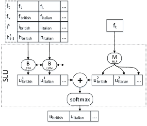
Figure 2: The SLU consists of two units. The first unit processes turn features $f_{t}$, per-value features $f_{v}$, original informs $i^{s}$ and belief from the previous turn $h^{s}_{t-1}$ by a bidirectional LSTM $B$ and outputs a vector $u^{1}$. The second unit maps turn features $f_{t}$ by an MLP $M$ (with two linear hidden layers of sizes 50 and 20 - effect of the first layer is to regularize information passed through the $M$) onto $u^{2}$. Softmaxed sum of those output vectors is used as a probability distribution of informed values $u^{s}_{t}$.

The SLU part of the tracker shown in Figure 2 is inspired by an architecture, proposed in ?), consisting of two separate units. The first unit works with value-independent features $f_{v_{i}}$ where slot values (like indian, italian, north, etc.) from the ontology are replaced by tags. This allows the unit to work with values that have not been seen during training.

The features are processed by a bidirectional LSTM $B$ (with 10 $tanh$ activated cells) which enables the model to compare the likelihoods of the values in the user utterance. Even though this is not a standard usage of the LSTM it has proved as crucial especially for estimating the None value which means that no value from the ontology was mentioned. The other benefit of this architecture is that it can weight its output $u^{1}$ according to how many ontology values have been detected during turn $t$.

However, not all ontology values can be replaced by tags because of speech-recognition errors or simply because the ontology representation is not the same as the representation in natural language (e.g. dontcare~it does not matter). For this purpose, the model uses a second unit that maps untagged features directly into a value vector $u^{2}$. Because of its architecture, the unit is able to work only with ontology values seen during training. At the end, outputs $u^{1}$, $u^{2}$ of the two units are summed together and turned into a probability distribution $u$ via softmax. Since all parts of our model ($R$, $F$, $G$, SLU) are differentiable, all parameters of the model can be trained jointly by gradient-descent methods.

3 Evaluation

Method. From each dialog in the dstc2_train data ($1612$ dialogs) we extracted training samples for the slots food, pricerange and area and used all of them to train each tracker. The development data dstc2_dev ($506$ dialogs) were used to select the $f_{t}$ and $f_{v}$ features. We took the $2000$ most frequent $f_{t}$ features and the $100$ most frequent $f_{v}$ features.

The cost that we optimized consists of a tracking cost, which is computed as a cross-entropy between a belief state $h^{s}_{t}$ and a goal annotation, and of an SLU cost, which is a cross-entropy between the output of the SLU $u_{t}^{s}$ and a semantic annotation. We did not use any regularization on model parameters. We trained the model for 30 epochs by SGD with the AdaDelta [Zeiler, 2012] weight-update rule and batch size 16 on fully unrolled dialogs. We use the model from the best iteration according to error rate on dstc2_dev. The evaluated model was an ensemble of 10 best trackers (according to the tracking accuracy on dstc2_dev) selected from $62$ trained trackers. All trackers used the same training settings with difference in initial parameter weights only). Our tracker did not track the name slot because there are no training data available for it. Therefore, we always set value for the name to None.

Results. This section briefly summarizes results of our tracker on dstc2_test (1117 dialogs) in all DSTC2 categories as can be seen in Table 1. We also provide evaluation of the tracker without specific components to measure their contribution in the overall accuracy.

	dstc2_test
	ASR	Batch ASR	Accuracy	L2	post DSTC	test validated
Hybrid Tracker – this work	$\surd$	$\surd$	.810	.318	$\surd$	$\surd$
DST2 stacking ensemble [Henderson et al., 2014a]	$\surd$	$\surd$	.798	.308	$\surd$	$\surd$
Hybrid Tracker – this work	$\surd$	$\surd$	.796	.338	$\surd$
?)	$\surd$	$\surd$	.784	.735
Hybrid Tracker – this work	$\surd$		.780	.356	$\surd$
?)	$\surd$		.775	.758
Hybrid Tracker without G – this work	$\surd$		.772	.368	$\surd$
Hybrid Tracker without M – this work	$\surd$		.770	.373	$\surd$
?)	$\surd$		.768	.346
Hybrid Tracker without bidir – this work	$\surd$		.763	.375	$\surd$
?)	$\surd$		.762	.436	$\surd$
YARBUS [Fix and Frezza-buet, 2015]	$\surd$		.759	.358	$\surd$
?)	$\surd$		.750	.416
Neural Belief Tracker [Mrkšić et al., 2016]	$\surd$		.73?	???	$\surd$
TL-DST [Lee and Stent, 2016]			.747	.451	$\surd$
Hybrid Tracker – this work			.746	.414	$\surd$
?)			.745	.433	$\surd$
?)			.739	.721
?)			.737	.406
Knowledge-based tracker [Kadlec et al., 2014]			.737	.429	$\surd$
?)			.735	.433
?)			.729	.452
?)			.726	.427
YARBUS [Fix and Frezza-buet, 2015]			.725	.440	$\surd$
?)			.718	.437
Focus baseline			.719	.464
HWU baseline			.711	.466

Table 1: Joint slot tracking accuracy and L2 (denotes the squared L2 norm between the estimated belief distribution and correct distribution) for various systems reported in the literature. The trackers that used ASR/Batch ASR have $\surd$ in the corresponding column. The results of systems that did not participate in DSTC2 are marked by $\surd$ in the “post DSTC” column. The first group shows results of trackers that used dstc test data for validation. The second group lists individual trackers that use ASR and Batch ASR features. The third group lists systems that use only the ASR features. The last group lists baseline systems provided by DSTC organizers.

In the standard categories using Batch ASR and ASR features, we set new state-of-the-art results. In the category without ASR features (SLU only) our tracker is slightly behind the best tracker [Lee and Stent, 2016].

For completeness, we also evaluated our tracker in the “non-standard” category that involves trackers using test data for validation. This setup was proposed in ?) where an ensemble was trained from all DSTC2 submissions. However, this methodology discards a direct comparison with the other categories since it can overfit to test data. Our tracker in this category is a weighted averaging ensemble of trackers trained for the categories with ASR and batch ASR.

We also tested contribution of specialization components $G$ and $M$ by training new ensembles of models without those components. Accuracy of the ensembles can be seen in Table 1. From the results can be seen that removing either of the components hurts the performance in a similar way.

In the last part of evaluation we studied importance of the bidirectional LSTM layer $B$ by ensembling models with linear layer instead. From the table we can see a significant drop in accuracy, showing the $B$ is a crucial part of our model.

4 Lessons learned

Originally we designed the special SLU unit $M$ with a sigmoid activation inspired by architecture of [Henderson et al., 2014b]. However, we found it difficult to train because gradients were propagated poorly through that layer causing its output to resemble priors of ontology values rather than probabilities of informing some ontology value based on corresponding ASR hypotheses as suggested by the network hierarchy. The problem resulted in an inability to learn alternative wordings of ontology values which are often present in the training data. One such example can be “asian food” which appears 16 times in the training data as a part of the best ASR hypothesis while 13 times it really informs about “asian oriental” ontology value. Measurements on dstc2_dev have shown that the SLU was not able to recognize this alias anytime. We managed to solve this training issue by simplifying the special SLU sigmoid to linear activation instead. The resulting SLU is able to recognize common alternative wordings as “asian food” appearing more than 10 times in training data, as well as rare alternatives like “anywhere” (meaning area:dontcare) appearing only 5 times in training data.

5 Conclusion

We have presented an end-to-end trainable belief tracker with modular architecture enhanced by differentiable rules. The modular architecture of our tracker outperforms other approaches in almost all standard DSTC categories without large modifications making our tracker successful in a wide range of input-feature settings.

References

- [Fix and Frezza-buet, 2015] Jeremy Fix and Herve Frezza-buet. 2015. YARBUS : Yet Another Rule Based belief Update System.
- [Henderson et al., 2014a] Matthew Henderson, Blaise Thomson, and Jason D. Williams. 2014a. The second dialog state tracking challenge. In Proceedings of the 15th Annual Meeting of the Special Interest Group on Discourse and Dialogue (SIGDIAL), pages 263–272, Philadelphia, PA, U.S.A., June. Association for Computational Linguistics.
- [Henderson et al., 2014b] Matthew Henderson, Blaise Thomson, and Steve Young. 2014b. Word-based dialog state tracking with recurrent neural networks. In Proceedings of the 15th Annual Meeting of the Special Interest Group on Discourse and Dialogue (SIGDIAL), pages 292–299, Philadelphia, PA, U.S.A., June. Association for Computational Linguistics.
- [Hochreiter and Schmidhuber, 1997] Sepp Hochreiter and Jürgen Schmidhuber. 1997. Long short-term memory. Neural computation, 9(8):1735–1780.
- [Kadlec et al., 2014] Rudolf Kadlec, Miroslav Vodolan, Jindrich Libovicky, Jan Macek, and Jan Kleindienst. 2014. Knowledge-based dialog state tracking. In Spoken Language Technology Workshop (SLT), 2014 IEEE, pages 348–353. IEEE.
- [Lee and Stent, 2016] Sungjin Lee and Amanda Stent. 2016. Task lineages: Dialog state tracking for flexible interaction. In Proceedings of the 17th Annual Meeting of the Special Interest Group on Discourse and Dialogue, pages 11–21, Los Angeles, September. Association for Computational Linguistics.
- [Lee et al., 2014] Byung-Jun Lee, Woosang Lim, Daejoong Kim, and Kee-Eung Kim. 2014. Optimizing generative dialog state tracker via cascading gradient descent. In Proceedings of the 15th Annual Meeting of the Special Interest Group on Discourse and Dialogue (SIGDIAL), pages 273–281, Philadelphia, PA, U.S.A., June. Association for Computational Linguistics.
- [Mrkšić et al., 2016] Nikola Mrkšić, Diarmuid Ó Séaghdha, Tsung-Hsien Wen, Blaise Thomson, and Steve Young. 2016. Neural belief tracker: Data-driven dialogue state tracking. arXiv preprint arXiv:1606.03777.
- [Ren et al., 2014] Hang Ren, Weiqun Xu, and Yonghong Yan. 2014. Markovian discriminative modeling for dialog state tracking. In Proceedings of the 15th Annual Meeting of the Special Interest Group on Discourse and Dialogue (SIGDIAL), pages 327–331, Philadelphia, PA, U.S.A., June. Association for Computational Linguistics.
- [Smith, 2014] Ronnie Smith. 2014. Comparative error analysis of dialog state tracking. In Proceedings of the 15th Annual Meeting of the Special Interest Group on Discourse and Dialogue (SIGDIAL), pages 300–309, Philadelphia, PA, U.S.A., June. Association for Computational Linguistics.
- [Sun et al., 2014] Kai Sun, Lu Chen, Su Zhu, and Kai Yu. 2014. The sjtu system for dialog state tracking challenge 2. In Proceedings of the 15th Annual Meeting of the Special Interest Group on Discourse and Dialogue (SIGDIAL), pages 318–326, Philadelphia, PA, U.S.A., June. Association for Computational Linguistics.
- [Vodolán et al., 2015] Miroslav Vodolán, Rudolf Kadlec, and Jan Kleindienst. 2015. Hybrid dialog state tracker. In Proceedings of NIPS 2015 Workshop on Machine Learning for Spoken Language Understanding and Interaction, pages 1–6, La Jolla, CA, USA. Neural Information Processing Systems Foundation.
- [Williams et al., 2016] Jason D. Williams, Antoine Raux, and Matthew Henderson. 2016. The dialog state tracking challenge series: A review. Dialogue & Discourse, 7(3):4–33.
- [Williams, 2014] Jason D. Williams. 2014. Web-style ranking and slu combination for dialog state tracking. In Proceedings of the 15th Annual Meeting of the Special Interest Group on Discourse and Dialogue (SIGDIAL), pages 282–291, Philadelphia, PA, U.S.A., June. Association for Computational Linguistics.
- [Yu et al., 2015] Kai Yu, Kai Sun, Lu Chen, and Su Zhu. 2015. Constrained Markov Bayesian Polynomial for Efficient Dialogue State Tracking. IEEE/ACM Transactions on Audio, Speech, and Language Processing, 23(12):2177–2188.
- [Zeiler, 2012] Matthew D. Zeiler. 2012. Adadelta: an adaptive learning rate method. arXiv preprint arXiv:1212.5701.