Spinon decay in the spin-1/2 Heisenberg chain with weak next nearest neighbour exchange

Abstract

Integrable models support elementary excitations with infinite lifetimes. In the spin-1/2 Heisenberg chain these are known as spinons. We consider the stability of spinons when a weak integrability breaking perturbation is added to the Heisenberg chain in a magnetic field. We focus on the case where the perturbation is a next nearest neighbour exchange interaction. We calculate the spinon decay rate in leading order in perturbation theory using methods of integrability and identify the dominant decay channels. The decay rate is found to be small, which indicates that spinons remain well-defined excitations even though integrability is broken.

1 Introduction

Integrable many-particle quantum systems are special in that they support stable elementary excitations. These typically are related in very complicated ways to the basic degrees of freedom. For example, in the Heisenberg antiferromagnet the elementary excitations are interacting spin-1/2 objects called spinons [1, 2]. Crucially, these elementary excitations are protected from decay into multi-particle excitations by the existence of local integrals of motion, even in cases where decay is kinematically allowed. In such situations application of integrability breaking perturbations has the immediate effect of inducing particle decay, and an important question is how large the corresponding decay rates are. If they are small, the elementary excitations of the integrable model will remain a good basis for describing the physics of the perturbed model. Such questions have been investigated in some detail for integrable quantum field theories [3, 4, 5, 6]. The case of integrable lattice models is considerably harder, and to the best of our knowledge has not been investigated so far. The added difficulty compared to field theory cases is that the description of the ground and excited states is more complicated (see below). The question of what effects weak integrability breaking perturbations have on the excitation spectrum of lattice models is also of importance in so-called mobile impurity approaches to the calculation of threshold singularity exponents in lattice models [7]. As pointed out in Ref. [8] in the context of the Hubbard model, there exist different formulations of mobile impurity models [9], which correspond to different choices of bases of elementary excitations. One may argue that for integrable models the “integrable” basis of elementary excitations ought to be the preferred choice. An obvious question is then whether this remains the case even if integrability is weakly broken. This is intimately related to how large the decay rate of the excitations is once a perturbation is applied. For the Hubbard model the available integrable model technology [10] does not currently permit to answer this question. In this work we therefore consider the simpler case of the spin-$1/2$ Heisenberg XXZ chain of length $L$ in a magnetic field $h$

$$\qquad H(J,\Delta,h)=J\sum_{j=1}^{L}\left(S_{j}^{x}S_{j+1}^{x}+S_{j}^{y}S_{j+1}^{y}+\Delta S_{j}^{z}S_{j+1}^{z}\right)-h\sum_{j=1}^{L}S_{j}^{z}\ .$$ (1)

Here $J<0$ and $S_{j}^{\alpha}$ are spin operators with commutation relations

$$[S_{i}^{\alpha},S_{j}^{\beta}]=i\delta_{ij}\varepsilon_{\alpha\beta\gamma}S_{i}^{\gamma}\ .$$ (2)

The spectrum of (1) is gapless for $\left|\Delta\right|\leq 1$ and $|h|<J(1+\Delta)$ [11, 12]. The model is integrable and elementary excitations over the ground state carry $S^{z}$ quantum number $1/2$ and are known as ”spinons” [1, 2, 11, 12]. A simple way of perturbing the model away from the integrable point is by introducing a next nearest neighbour interaction

$$\delta H=\kappa\sum_{j}S_{j}^{z}S_{j+2}^{z}\ .$$ (3)

This interaction destroys integrability, but still commutes with the total spin operator along the z-axis $S^{z}=\sum_{j}S_{j}^{z}$. Hence the z-component of the total spin remains a good quantum number. In presence of the perturbation spinons cease to be exact elementary excitations and we expect them to acquire a finite life-time. Using Fermi’s golden rule for small perturbations the decay rate can be expressed in the form

$$\Gamma=2\pi\sum_{f}\left|\mathcal{M}(i\to f)\right|^{2}\rho_{f}(E_{i})\;\delta_{p_{f},p_{i}}$$ (4)

where $E_{f}$ and $p_{f}$ ($E_{i}$ and $p_{i}$) are the energy and momentum of the final (initial) state [13], $\rho_{f}(E)$ the density of states of the final state and the matrix element $\mathcal{M}$ is given by

$$\mathcal{M}=\left<f\right|\delta H\left|i\right>\ .$$ (5)

We are interested in the case where the initial state is an exact one-spinon eigenstate of (1), while the final state is any exact eigenstate of the unperturbed system.

Most of our analysis will focus on the isotropic Heisenberg model at $\Delta=1$ and $h>0$. Other values of $\Delta$ can be treated in the same way and $h<0$ by considering the spin overturned sector. The outline of this paper is as follows. Section 2 presents a brief summary of the Bethe Ansatz solution of the Heisenberg model. We then describe the excited states that contribute to the decay rate in section 3. We then use the Algebraic Bethe Ansatz to obtain explicit expressions for the matrix elements describing the spinon decay, cf. 4. In section 5 we then numerically determine the contributions of various decay channels to the decay rate. We end with a discussion of our results in section 6.

2 Bethe Ansatz solution of the XXX-chain

2.1 Coordinate Bethe Ansatz

Eigenstates of the XXZ Hamiltonian (1) can be constructed by means of the Bethe Ansatz [14] for any value of the anisotropy $\Delta$. As $S^{z}$ commutes with the XXZ Hamiltonian and with the perturbation $\delta H$, it is convenient to work in a sector with a fixed number of down-spins $N$ with respect to the ferromagnetic state

$$\left|0\right>:=\left|S^{z}=\frac{L}{2}\right>=\bigotimes_{j=1}^{L}\left|\uparrow\right>_{j}\ ,$$ (6)

which will be used as a reference state in the following. Energy eigenstates with $N$ down-spins take the form

$$\left|N\right>=\sum_{j_{1},\dots,j_{N}=1}^{L}a(j_{1},\dots,j_{N})\prod_{a=1}^{N}S_{j_{a}}^{-}\left|0\right>\ ,$$ (7)

where $1\leq j_{1}<j_{2}<\dots<j_{N}\leq L$. The wave functions have Bethe Ansatz form [11, 12, 15, 16]

$$a(j_{1},\dots,j_{N})= \sum_{P\in S_{N}}(-1)^{[P]}\mathcal{A}_{P}\;\text{exp}\left(i\sum_{a=1}^{N}k_{Pa}j_{a}\right)\ ,$$

$$\mathcal{A}_{P}= \prod_{a<b}\left(e^{i(k_{P_{a}}+k_{P_{b}})}+1-2\Delta e^{ik_{P_{a}}}\right).$$ (8)

The energy of the state with wave function (8) is given by

$$E =J\sum_{a=1}^{N}(\cos{k_{a}}-\Delta)-h\left(\frac{L}{2}-N\right).$$ (9)

2.2 Bethe equation for the XXX model

Imposing periodic boundary conditions on the wave functions (8) leads to quantization conditions for the wave numbers $k_{a}$ known as Bethe Ansatz equations

$$e^{ik_{a}L}=\prod_{a\neq b}^{N}\left[-\frac{2\Delta e^{ik_{a}}-e^{ik_{a}+ik_{b}}-1}{2\Delta e^{ik_{b}}-e^{ik_{a}+ik_{b}}-1}\right].$$ (10)

From here on we set $\Delta=1$. It is convenient to introduce rapidity variables $\lambda_{a}$ defined by

$$e^{ik_{a}}=\frac{\lambda_{a}-i/2}{\lambda_{a}+i/2}.$$ (11)

In terms of the rapidity variables the Bethe Ansatz equations read

$$\left(\frac{\lambda_{a}-i/2}{\lambda_{a}+i/2}\right)^{L}=\prod_{\begin{subarray}{c}b=1\\ b\neq a\end{subarray}}^{N}\frac{\lambda_{a}-\lambda_{b}-i}{\lambda_{a}-\lambda_{b}+i}\ ,\ a=1,\dots,N.$$ (12)

A standard way of analyzing (12) is by employing the string hypothesis. This assumes that all solutions of (12) are composed of strings of the form

$$\lambda^{n,j}_{\alpha}=\lambda^{n}_{\alpha}+\frac{i}{2}(n+1-2j)+\delta^{n,j}_{\alpha}\ ,\quad j=1,\dots,n.$$ (13)

Here $\delta^{n,j}_{\alpha}$ are deviations from “ideal” strings and are assumed to be exponentially small in system size. Let us now consider a solution to (12) that contains $M_{n}$ strings of length $n$ with corresponding string centres $\lambda^{n}_{\alpha}$ (this implies that $\sum_{n}M_{n}n=N$). Substituting (13) into (12) and neglecting the deviations we obtain a set of coupled equations for the set $\{\lambda^{n}_{\alpha}\}$. Taking logarithms we arrive at

$$L\theta\left(\frac{\lambda^{n}_{\alpha}}{n}\right)=2\pi I^{n}_{\alpha}+\sum_{(m,\beta)\neq(n,\alpha)}\theta_{nm}(\lambda^{n}_{\alpha}-\lambda^{m}_{\beta}).$$ (14)

Here $I^{n}_{\alpha}$ are integer or half-odd integers numbers (arising from taking logarithms), $\theta(x)=2{\rm arctan}(2x)$, and

$$\theta_{nm}(x)=\begin{cases}\theta\big{(}\frac{x}{2n}\big{)}+2\sum_{j=1}^{n-1}\theta\big{(}\frac{x}{2j}\big{)}&\text{for }m=n\\ \theta\big{(}\frac{x}{|n-m|}\big{)}+2\theta\big{(}\frac{x}{|n-m|+2}\big{)}+\ldots+2\theta\big{(}\frac{x}{n+m-2}\big{)}+\theta\big{(}\frac{x}{n+m}\big{)}&\text{for }m\neq n\end{cases}.$$ (15)

Equations (14) are called Takahashi’s equations. They relate the solutions of the BAE to a set of integer of half-odd integer numbers, which therefore can be considered as quantum numbers of our problem. The permitted ranges of the $I^{n}_{\alpha}$ are [11]

$$|I^{n}_{\alpha}|\leq\frac{1}{2}\left[L-1-\sum_{m=1}^{\infty}\left(2{\rm min}(m,n)-\delta_{n,m}\right)M_{m}\right].$$ (16)

Energy and momentum of solutions to (14) are given by

$$E = \sum_{m=1}^{\infty}\sum_{\beta=1}^{M_{m}}\left(-\pi Ja_{n}(\lambda^{m}_{\beta})+mh\right)-\frac{hL}{2}\ ,$$

$$P = \pi+\sum_{m=1}^{\infty}\sum_{\beta=1}^{M_{m}}\frac{2\pi I^{m}_{\beta}}{L}$$ (17)

where we have defined

$$a_{n}(x)=\frac{1}{2\pi}\frac{n}{x^{2}+(n/2)^{2}}\ .$$ (18)

All solutions to Takahashi’s equations correspond to highest weight states of the spin SU(2) algebra [2]

$$S^{+}|\{\lambda^{n}_{\alpha}\}\rangle=0.$$ (19)

A complete set of energy eigenstates is then obtained by acting with the spin lowering operator on these highest weight states

$$\left(S^{-}\right)^{m}|\{\lambda^{n}_{\alpha}\}\rangle\ ,\quad m=0,1,\dots,L-2\sum_{n}nM_{n}.$$ (20)

3 Low lying excitations and spectrum

In order to have access to single-spinon excitations we need to consider odd chain lengths $L$. For even values of $L$ the lowest excitations involve at least two spinons [2].

3.1 One particle and one hole excitations

For odd $L$ with an odd number $N$ of down spins there are two degenerate lowest energy states. They are obtained by considering real solutions (1-strings) to the Bethe Ansatz equations and choosing either

$$I^{1}_{\alpha}=-\frac{N}{2}+\alpha\ ,\quad\alpha=1,\dots,N,$$ (21)

or

$$I^{1}_{\alpha}=-\frac{N}{2}+1+\alpha\ ,\quad\alpha=1,\dots,N,$$ (22)

The corresponding configurations of half-odd integers for $N=11$ look as follows:

The energy density $e(h)$ of these two states in the thermodynamic limit

$$L,N\to\infty,\frac{N}{L}=n=\text{fixed}$$ (23)

can be expressed in terms of the solution of a linear integral equation for the root density $\rho_{1}(\lambda)$, cf. Ref. [11]

$$\rho_{1}(\lambda)=a_{1}(\lambda)-\int_{-B}^{B}\text{d}\eta\;a_{2}\left(\lambda-\eta\right)\ \rho_{1}(\eta).$$ (24)

Here the integration boundary $B$ is determined by the density of down spins $n$ through

$$\int_{-B}^{B}\text{d}\lambda\;\rho_{1}(\lambda)=n.$$ (25)

The energy per site is then given by

$$e(h)=\int_{-B}^{B}\text{d}\lambda\;\rho_{1}(\lambda)\varepsilon^{(0)}_{1}(\lambda)\ ,$$ (26)

where

$$\varepsilon^{(0)}_{1}(\lambda)=-J\pi a_{1}(\lambda)+h\ .$$ (27)

The two states above are particular limits of one-parameter particle-like and hole-like excitations. The particle excitation corresponds to $I^{1}_{\alpha}$ configurations of the form

whereas the hole-like excitation is obtained by promoting one half-odd integer $I_{\alpha}^{1}$ in the ground state configuration to the “Fermi edge” that has one fewer half-odd integer:

Both types of excitations involve a single parameter: $I^{p}$ for the particle excitation and $I^{h}$ for the hole excitation. For asymptotically large system sizes $L$ the energies and momenta of these excitations are given by [11]

$$E^{p} =Le+\varepsilon_{1}(\lambda^{p})+o(1),\qquad\left|\lambda^{p}\right|>B\ ,$$ (28)

$$P^{p} =\pi+2\pi\int_{0}^{\lambda^{p}}\text{d}\lambda\;\rho_{1}(\lambda)+{\cal O}(L^{-1})\ ,$$ (29)

$$E^{h} =Le-\varepsilon(\lambda^{h})+o(1),\qquad\left|\lambda^{h}\right|<B\ ,$$ (30)

$$P^{h} =\pi-2\pi\int_{0}^{\lambda^{h}}\text{d}\lambda\;\rho_{1}(\lambda)+{\cal O}(L^{-1})\ ,$$ (31)

where the dressed energy $\epsilon_{1}(\lambda)$ is a solution to the linear integral equation

$$\varepsilon_{1}(\lambda)=\varepsilon^{(0)}_{1}(\lambda)-\frac{1}{2\pi}\int_{-B}^{B}\text{d}\mu\;\ a_{2}(\mu-\lambda)\ \varepsilon_{1}(\mu).$$ (32)

The rapidities $\lambda^{p}$ and $\lambda^{h}$ are continuous parameters above and below the “Fermi-edge” respectively. They are related to the parameters $I^{p}$ and $I^{h}$ through Takahashi’s equations (14).

The excitation energy for a one-spinon excitation can now be extracted by simply subtracting the extensive part of the energy (which equals the ground state energy per site of the Heisenberg chain), which allows us to extract the spinon energy and momentum

$$\epsilon_{s}(\lambda)=|\varepsilon_{1}(\lambda)|\ ,\qquad p_{s}(\lambda)=\pi+2\pi\ {\rm sgn}(|\lambda|-B)\int_{0}^{\lambda}d\mu\ \rho_{1}(\mu)\ .$$ (33)

The corresponding dispersion relation is plotted for several values of magnetic field $h$ in Fig. 1 where the value for the magnetic field is fixed by imposing $\varepsilon_{1}(B)=0$.

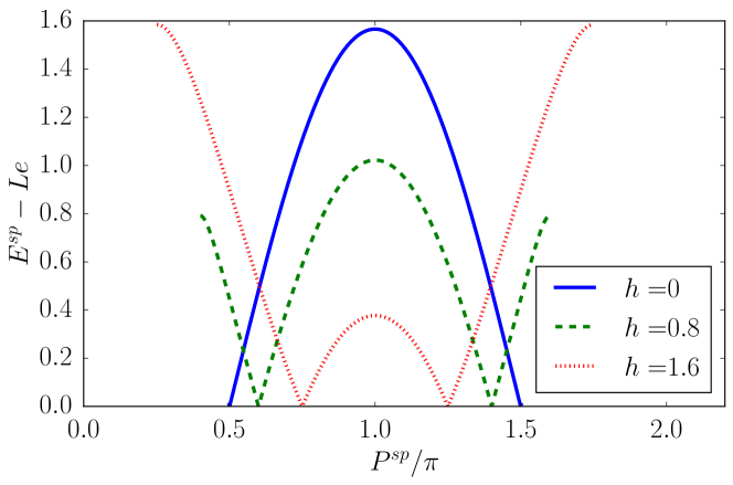
Figure 1: Energy-momentum dispersion of the one-parameter excitations for different values of the magnetic field h.

We note that by construction the spinon dispersion is identical to the one extracted from the two-spinon excitation of the Heisenberg model with even chain lengths $L$, apart from a shift in momentum by $\pi$.

3.2 Excitations involving several particles and/or holes

As $\delta H$ commutes with $S^{z}$, the decay of the single-particle (hole) excitation described above can only involve excited states with the same $S^{z}$ quantum number. These are obtained in the following ways:

1. One can consider solutions of Takahashi’s equations only involving 1-strings. These will involve additional particle-hole excitations on top of the 1-spinon excitation constructed above.

2. One can consider solutions of Takahashi’s equations involving $n$-strings with $n\geq 2$. As a result of the magnetic field these excitations have a gap.

3. One can consider excitations of the form (20) that are not SU(2) highest-weight states. These again have a gap for $h>0$ because

   $$[S^{-},H(J,\Delta,h)]=-hS^{-}$$ (34)

As we are dealing with an interacting theory, this leaves us with an infinite number of possible decay channels, i.e. even to first order in perturbation theory in $\kappa$, a single spinon can decay into excitations involving $3,5,7,\dots$ particles. As in one dimension the accessible phase space shrinks with the number of particles involved [17], it is reasonable to assume that the dominant decay channels will involve excitations with low numbers of particles. In the following we will focus on excitations involving $3$ particles. We have considered a class of five-particle excitations where we excite two particle- and hole-type excitations in addition to the one-spinon excitation, and found the corresponding decay rate to be smaller (see section 5).

3.2.1 “pph-excitation”

This excitation involves only 1-strings and corresponds to configurations of the (half-odd) integers $I^{1}_{\alpha}$ looking as follows

States of this kind can be thought of as a sub-class of 3-spinon excitations that involves two particles and one hole, which are parametrized by $I^{h}$ and $I^{p}_{1,2}$ respectively (or equivalently by the corresponding rapidities $\lambda^{h}$, $\lambda^{p}_{1,2}$). Energy and momentum of this excitation are given by

$$E^{pph} =Le+\epsilon_{s}(\lambda_{1}^{p})+\epsilon_{s}(\lambda_{2}^{p})+\epsilon_{s}(\lambda^{h})+o(1)\ ,$$ (35)

$$P^{pph} =p_{s}(\lambda^{p}_{1})+p_{s}(\lambda^{p}_{2})+p_{s}(\lambda^{h})+{\cal O}(L^{-1})\ ,$$ (36)

where $\epsilon_{s}(\lambda)$ and $p_{s}(\lambda)$ are defined in (33). The excitation energy is obtained subtracting the ground state energy, and the corresponding continuum of 3-spinon excited states is shown in Fig. 2(a). The grey shading reflects the density of excitations at given values of energy and momentum. Darker regions correspond to higher densities. The intensity of the shading is obtained by considering large but finite $L$ and varying $I^{h}$ and $I^{p}_{1,2}$ over all allowed values for a given excitation, and calculating approximate values of $\lambda^{h},\lambda^{p}_{1,2}$ by solving the equation

$$p_{s}(\lambda^{h})=\frac{2\pi I^{h}}{L}\ ,\quad p_{s}(\lambda^{p}_{j})=\frac{2\pi I^{p}_{j}}{L}\ ,\ j=1,2.$$ (37)

The corresponding approximate excitation energy is then obtained by substituting these values into (36). Each set $\{I^{h},I^{p}_{1,2}\}$ provides one point in the $P^{pph}$-$E^{pph}$-plane and the collection of all these points generates a shading that reflects the density of states.

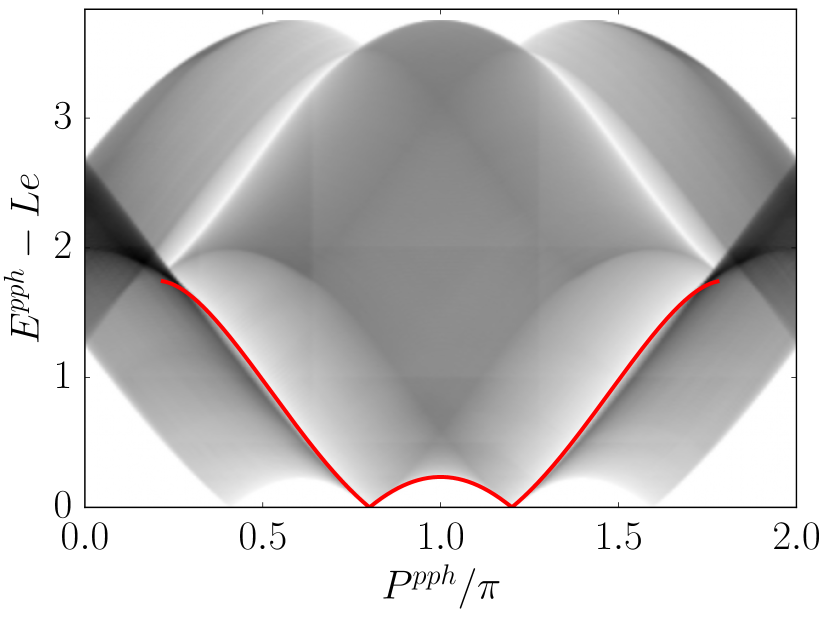
(a)

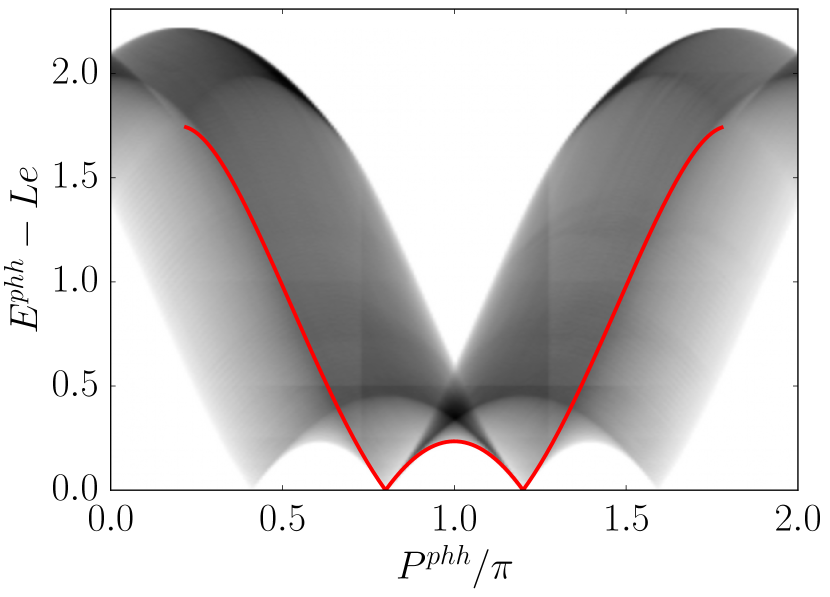
(b)

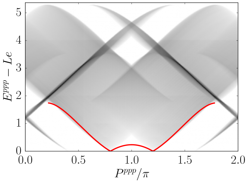
(c)

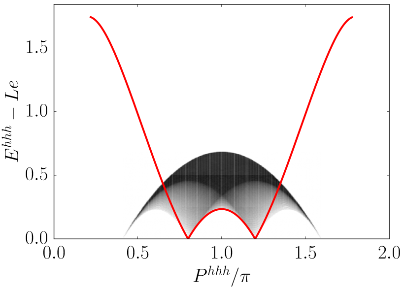
(d)

Figure 2: Excitation continua (grey) for (a) two particle one hole (b) one particle two holes (c) three particle and (d) three holes at magnetization $m=3/10$. The 1-spinon dispersion is shown in red. The shading of the continuum reflects the density of states (see main text). Decay of the single spinon is kinematically allowed in part of the Brillouin zone.

We see that for momenta $\pi(\frac{1}{2}+m)<p_{s}(\lambda)<\pi(\frac{3}{2}-m)$ decay of the 1-spinon excitation is kinematically forbidden, while it is allowed for some values in the regions $p_{s}(\lambda)>\pi(\frac{3}{2}-m)$ and $p_{s}(\lambda)<\pi(\frac{1}{2}+m)$.

3.2.2 “phh-excitation”

This excitation involves only 1-strings and corresponds to configurations of the (half-odd) integers $I^{1}_{\alpha}$ looking as follows

States of this kind are a sub-class of 3-spinon excitations that involves one particle and two holes, which are parametrized by $I^{p}$ and $I^{h}_{1,2}$ or equivalently by the corresponding rapidities $\lambda^{p},\lambda^{h}_{1,2}$. Energy and momentum of this excitation are given by

$$E^{phh} =Le+\epsilon_{s}(\lambda^{p})+\epsilon_{s}(\lambda^{h}_{1})+\epsilon_{s}(\lambda^{h}_{2})+o(1)\ ,$$ (38)

$$P^{phh} =p_{s}(\lambda^{p})+p_{s}(\lambda^{h}_{1})+p_{s}(\lambda^{h}_{2})+{\cal O}(L^{-1})\ ,$$ (39)

where $\epsilon_{s}(\lambda)$ and $p_{s}(\lambda)$ are defined in (33). The excitation energy is again obtained by subtracting the ground state energy and is shown as a function of the total momentum in Fig. 2(b).

3.2.3 “ppp-excitations”

This excitation involves only 1-strings and corresponds to configurations of the (half-odd) integers $I^{1}_{\alpha}$ looking as follows

States of this kind are a sub-class of 3-spinon excitations that involves three particles. Energy and momentum of this excitation are

$$E^{ppp} =Le+\sum_{j=1}^{3}\epsilon_{s}(\lambda_{j}^{p})+o(1)\ ,$$ (40)

$$P^{ppp} =\sum_{j=1}^{3}p_{s}(\lambda^{p}_{j})+{\cal O}(L^{-1}),$$ (41)

where $\epsilon_{s}(\lambda)$ and $p_{s}(\lambda)$ are defined in (33). The excitation energy is again obtained by subtracting the ground state energy and is shown as a function of the total momentum in Fig. 2(c).

3.2.4 “hhh-excitations”

This excitation involves only 1-strings and corresponds to configurations of the (half-odd) integers $I^{1}_{\alpha}$ looking as follows

States of this kind are a sub-class of 3-spinon excitations that involves three holes. Energy and momentum of this excitation are

$$E^{hhh} =Le+\sum_{j=1}^{3}\epsilon_{s}(\lambda_{j}^{h})+o(1)\ ,$$ (42)

$$P^{hhh} =\sum_{j=1}^{3}p_{s}(\lambda^{h}_{j})+{\cal O}(L^{-1}),$$ (43)

where $\epsilon_{s}(\lambda)$ and $p_{s}(\lambda)$ are defined in (33). The excitation energy is again obtained by subtracting the ground state energy and is shown as a function of the total momentum in Fig. 2(d).

3.2.5 Excitations involving a single 2-string

We now turn to the simplest excitation involving a single 2-string. This corresponds to solutions of (14) with $M_{1}=N-2$, $M_{2}=1$ and configurations of the half-odd integers $I^{1}_{\alpha}$, $I^{2}_{1}$ of the kind

We note that the permitted values for $I^{2}_{1}$ have range

$$|I^{2}_{1}|\leq\frac{1}{2}\left[L-2N\right].$$ (44)

The excitation is parametrized by the two half-odd integers $I^{p},I^{2}_{1}$ or equivalently the corresponding rapidities $\lambda^{p},\lambda^{s}$. Energy and momentum of this excitation are given by

$$E^{2sp} =Le+\epsilon_{s}(\lambda^{p})+\varepsilon_{2}(\lambda^{s})\,,\qquad\left|\lambda^{p}\right|>B\ ,$$ (45)

$$P^{2sp} =p_{s}(\lambda^{p})+p_{2}(\lambda^{s})\ ,$$ (46)

where $\varepsilon_{2}$ and $p_{2}(\lambda)$ are given by [11]

$$\varepsilon_{2}(\lambda) = h+\int_{|\mu|>B}\text{d}\mu\;a_{1}(\lambda-\mu)\ \varepsilon_{1}(\mu)\ ,$$

$$p_{s}(\lambda) = \theta\Big{(}\frac{\lambda}{2}\Big{)}-\int_{-B}^{B}d\mu\ \theta_{21}(\lambda-\mu)\ \rho_{1}(\mu).$$ (47)

Excitation continua that encompass the two-particle continuum (46) are obtained by adding particle-hole excitations, e.g.

$$E^{2s3p2h} =Le+\sum_{j=1}^{3}\epsilon_{s}(\lambda^{p}_{j})+\sum_{k=1}^{2}\epsilon_{s}(\lambda^{h}_{k})+\varepsilon_{2}(\lambda^{s})\,,\qquad\left|\lambda^{h}_{j}\right|<B<\left|\lambda^{p}_{k}\right|\ ,$$ (48)

$$P^{2s3p2h} =\sum_{j=1}^{3}p_{s}(\lambda^{p}_{j})+\sum_{k=1}^{2}p_{s}(\lambda^{h}_{k})+p_{2}(\lambda^{s})\ .$$ (49)

The continuum (49) is shown in Fig. 3 for several magnetizations. We see that the single spinon excitation cannot decay into the 2-string excitation for kinematic reasons.

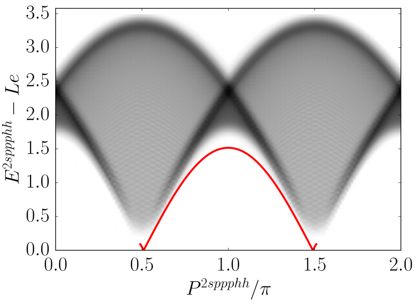
(a)

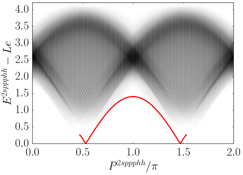
(b)

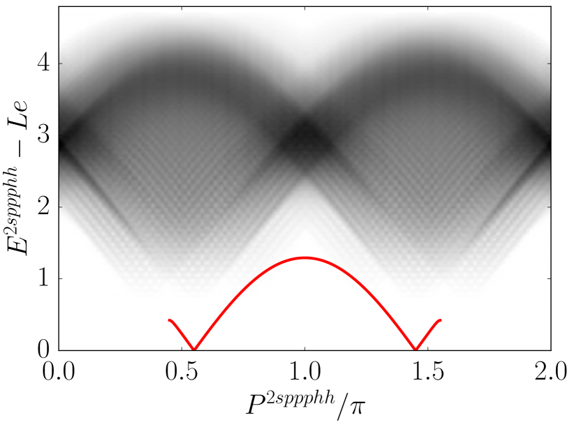
(c)

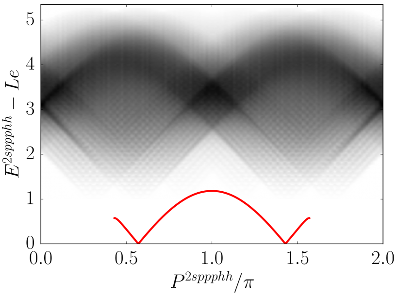
(d)

Figure 3: One two-string and $3p2h$ excitation continuum (grey) at magnetization (a) $m=0.01$, (b) $m=0.03$, (c) $m=0.05$ and (d) $m=0.07$, (the corresponding magnetic fields are $h=0.09$, $h=0.26$, $h=0.42$ and $h=0.58$ respectively). The 1-spinon dispersion is shown in red. The shading of the continuum reflects the density of states (see main text). Decay of the single spinon is kinematically not allowed.

If we keep on adding particle-hole excitation at small magnetic fields decay of the 1-spinon excitation will eventually become kinematically allowed. However, the decay rate is then expected to be negligible on the basis of aforementioned phase-space arguments, cf. Ref. [17].

3.2.6 Excitations involving longer strings

Excitations involving longer strings have larger gaps at finite magnetic fields [11]. We expect contributions from decay channels involving such excitations to be small for the same reasons we put forward in the 2-string case above.

3.2.7 Excitations that are not highest weight states

As mentioned above, excitations which are not highest weight states have gaps that are proportional to the magnetic field $h$. Nevertheless, decay of a single spinon into excitations that are not highest weight states will generally be allowed at sufficiently small $h$. As an example let us consider highest-weight states with $M_{1}=N-1$, $M_{n\geq 2}=0$. The lowest energy states in this sector correspond to integers

$$I^{1}_{\alpha}=-\frac{N}{2}+\alpha\ ,\quad\alpha=1,\dots,N,$$ (50)

or

$$I^{1}_{\alpha}=-\frac{N}{2}-1+\alpha\ ,\quad\alpha=1,\dots,N,$$ (51)

In complete analogy to our discussion above, these can be viewed as particular limits of a 1-spinon excitation. Acting with the spin lowering operator gives a 1-parameter excited state with a dispersion that equals the 1-spinon dispersion shifted upwards in energy by $h$. Hence decay of our 1-spinon excitation into this particular descendant state is kinematically not allowed. However, if we add an additional particle-hole pair the situation changes. Let us consider configurations of integers such as

States of this kind can be thought of as a sub-class of 3-spinons. Energy and momentum of the excitation obtained by acting with the spin-lowering operator on this state are given by

$$E^{pph}_{\rm desc} =Le+\epsilon_{s}(\lambda_{1}^{p})+\epsilon_{s}(\lambda_{2}^{p})+\epsilon_{s}(\lambda^{h})+h+o(1)\ ,$$ (52)

$$P^{pph}_{\rm desc} =\pi+p_{s}(\lambda^{p}_{1})+p_{s}(\lambda^{p}_{2})+p_{s}(\lambda^{h})+{\cal O}(L^{-1})\ .$$ (53)

Inspection of Fig. 2(a) shows that decay of the 1-spinon excitation into this continuum is kinematically allowed at sufficiently weak fields. However, as shown in A this decay is strongly suppressed for large system sizes $L$.

4 Algebraic Bethe Ansatz and Derivation of the Matrix Element

4.1 Algebraic Bethe Ansatz

In order to determine decay rates we require matrix elements of the perturbing operator between energy eigenstates. These can be obtained using the Algebraic Bethe Ansatz [12]. In the following we will first consider the XXZ case with anisotropy parameter $\Delta=\cos\gamma$ and only later specialize to the isotropic limit $\Delta=1$. A key object is the monodromy matrix

$$T(\lambda)=\begin{pmatrix}A(\lambda)&B(\lambda)\\ C(\lambda)&D(\lambda)\end{pmatrix}\ ,$$ (54)

where $A,B,C,D$ are operators acting on the Hilbert space of the chain and $\lambda$ is known as spectral parameter. The mondromy matrix fulfils the Yang-Baxter equation

$$R(\lambda-\mu)(T(\lambda)\otimes 1) (1\otimes T(\mu))=$$

$$(1\otimes T(\mu))(T(\lambda)\otimes 1)R(\lambda-\mu)\ ,$$ (55)

where the $R$-matrix has the form

$$R(\lambda,\mu)=\begin{pmatrix}1&0&0&0\\ 0&b(\lambda,\mu)&c(\lambda,\mu)&0\\ 0&c(\lambda,\mu)&b(\lambda,\mu)&0\\ 0&0&0&1\end{pmatrix}.$$ (56)

Here we have defined

$$b(\lambda) =\frac{\sinh(\lambda)}{\sinh(\lambda+i\gamma)}$$ (57)

$$c(\lambda) =\frac{\sinh(i\gamma)}{\sinh(\lambda+i\gamma)}$$ (58)

The Yang-Baxter algebra determines intertwining relations for the operators $A,B,C,D$. Eigenstates of (1) can be constructed as

$$\left|\lambda_{1},\dots,\lambda_{N}\right>=\prod_{i=1}^{N}B(\lambda_{i})\left|0\right>\ ,$$ (59)

where the set of rapidities $\{\lambda_{i}\}_{i\in\{1,\dots,N\}}$ are solutions to the Bethe equations

$$\frac{a(\mu_{j})}{d(\mu_{j})}=\prod_{k\neq j}\frac{b(\mu_{k}-\mu_{j})}{b(\mu_{j}-\mu_{k})}\ ,\quad j=1,\dots,N.$$ (60)

The reference state $\left|0\right>$ satisfies

$$A(\lambda)\left|0\right>=\left|0\right> D(\lambda)\left|0\right>=d(\lambda)\left|0\right> C(\lambda)\left|0\right>=0\ .$$ (61)

The functions $a(\mu)$ and $d(\mu)$ are given by

$$a(\mu)=1 d(\mu)=\Big{(}b(\mu-i\frac{\gamma}{2})\Big{)}^{L}.$$ (62)

The isotropic limit $\Delta=1$ corresponds to taking $\gamma\to 0$, while rescaling the spectral parameters

$$\mu_{j}=\gamma\lambda_{j}\ ,\quad\lambda_{j}\ {\rm fixed}.$$ (63)

This recovers the Bethe Ansatz equations (12) from (60). The global spin lowering operator is obtained as [2]

$$-i\lim_{\lambda\to\infty}\lambda\,B(\lambda)=S^{-}.$$ (64)

4.2 Determinant Formulas for Matrix Elements in the XXZ chain

The Algebraic Bethe Ansatz provides a convenient setting for calculating scalar products as well as the norm of Bethe states [18, 19, 20]. Matrix elements can be analyzed by utilizing the expression of local spin operators $\sigma_{j}^{z}$ in terms of the operators $A,B,C,D$, cf. Ref. [21]. With the help of these relations matrix elements of spin operators $S^{\alpha}_{j}$ between eigenstates of the XXZ Hamiltonian were derived in Ref. [21], and general operators were considered in Ref. [22]. Explicit expressions for the operator $S^{z}_{j}S^{z}_{j+1}$ were obtained in Ref. [23]. Following the derivation of Ref. [23] we obtain (see B for details)

$$\sum_{j}\left<\lambda_{1},\dots,\lambda_{N}\right|S_{j}^{z}S_{j+2}^{z}\left|\mu_{1},\dots,\mu_{M}\right>=$$

$$Le^{iP_{\{\lambda\}}+2iP_{\{\mu\}}}\delta_{P_{\{\lambda\}},P_{\{\mu\}}}\delta_{M,N}\left\{-\phi(i\gamma)\frac{\prod_{k}\phi(\lambda_{k}+i\gamma/2)^{2}\phi(\mu_{k}+i\gamma/2)\phi(\mu_{k}-i\gamma/2)^{-3}}{\prod_{a>b}\phi(\lambda_{b}-\lambda_{a})\prod_{b>a}\phi(\mu_{b}-\mu_{a})}\right.$$

$$\times\sum_{n}A_{n}\left(\text{det}\left(G_{n}^{(1)}+B_{n}^{(1)}\right)+\text{det}\left(G_{n}^{(2)}+B_{n}^{(2)}\right)-\text{det}\left(G^{(1)}\right)-\text{det}\left(G^{(2)}\right)\right)$$

$$\hskip 28.45274pt-\frac{1}{2}\frac{\prod_{k}\phi(\lambda_{k}+i\gamma/2)^{3}\phi(\mu_{k}-i\gamma/2)^{-3}}{\prod_{a>b}\phi(\lambda_{b}-\lambda_{a})\prod_{a<b}\phi(\mu_{b}-\mu_{a})}$$

$$\left.\hskip 56.9055pt\times\sum_{n=1}\sum_{m\neq n}A_{nm}\left[\text{det}\left(G_{nm}+B_{nm}\right)-\text{det}\left(G_{nm}\right)\right]\right\}\ .$$ (65)

Here $P_{\{\lambda\}}$ is the total momentum of the state parametrized by the rapidities $\{\lambda_{j}\}$

$$P_{\{\lambda\}}=\sum_{j=1}^{N}\left[\pi+\ln\left(\frac{\lambda_{j}+\frac{i\gamma}{2}}{\lambda_{j}-\frac{i\gamma}{2}}\right)\right],$$ (66)

and

$$H_{ab} =\frac{\phi(i\gamma)}{\phi(\lambda_{a}-\mu_{b})}\Big{(}a(\mu_{b})\prod_{k\neq a}\phi(\lambda_{k}-\mu_{b}+i\gamma)-d(\mu_{b})\prod_{k\neq a}\phi(\lambda_{k}-\mu_{b}-i\gamma)\Big{)},$$ (67)

$$(G^{(1)}_{n})_{ab} =\begin{cases}H_{ab}&b\neq n\\ \frac{\phi(i\gamma)\phi(2\lambda_{a})}{\phi(\lambda_{a}-\frac{i\gamma}{2})^{2}\phi(\lambda_{a}+\frac{i\gamma}{2})^{2}}&b=n\end{cases}\ ,$$ (68)

$$(G^{(2)}_{n})_{ab} =\begin{cases}H_{ab}&b\neq n\\ \frac{\partial^{2}}{\partial x^{2}}\left(\frac{\phi(i\gamma)}{\phi(\lambda_{a}-x)\phi(\lambda_{a}-x+i\gamma)}\right)\big{|}_{x=\frac{i\gamma}{2}}&b=n\end{cases}\ ,$$ (69)

$$(B^{(1)}_{n})_{ab} =(1-\delta_{bn})d(\mu_{b})\prod_{i\neq n}\phi(\mu_{i}-\mu_{b}+i\gamma)\phi(\mu_{b}+i\gamma/2)$$

$$\times\left(\frac{\phi^{\prime}(i\gamma)}{\phi(i\gamma)}-\sum_{d\neq n}\frac{\phi(i\gamma)}{\phi(\mu_{d}-i\gamma/2)\phi(\mu_{d}+i\gamma/2)}+\sum_{d\neq m,n}\frac{\phi^{\prime}(\mu_{d}-i\gamma/2)}{\phi(\mu_{d}-i\gamma/2)}\right.$$

$$\left.-\sum_{b}\frac{\phi^{\prime}(\lambda_{b}+i\gamma/2)}{\phi(\lambda_{b}+i\gamma/2)}+\frac{\phi(i\gamma)}{\phi(\mu_{m}+i\gamma/2)\phi(\mu_{m}-i\gamma/2)}\right)\ ,$$ (70)

$$(B^{(2)}_{n})_{ab} =(1-\delta_{bn})\frac{1}{2}d(\mu_{b})\prod_{i\neq n}\frac{\phi(\mu_{i}-\mu_{b}-i\gamma)\phi(\mu_{b}+i\gamma)\phi(i\gamma)}{\phi(\lambda_{a}+i\gamma/2)\phi(\lambda_{a}-i\gamma/2)}\ .$$ (71)

$$(G_{nm})_{ab} =\begin{cases}H_{ab}&b\neq m,n\\ \frac{\phi(i\gamma)\phi(2\lambda_{a})}{\phi(\lambda_{a}-\frac{i\gamma}{2})^{2}\phi(\lambda_{a}+\frac{i\gamma}{2})^{2}}&b=m\\ \frac{\partial^{2}}{\partial x^{2}}\left(\frac{\phi(i\gamma)}{\phi(\lambda_{a}-x)\phi(\lambda_{a}-x+i\gamma)}\right)\big{|}_{x=\frac{i\gamma}{2}}&b=n\end{cases}$$ (72)

$$(B_{nm})_{ab} =(1-\delta_{bm})(1-\delta_{bn})d(\mu_{b})\prod_{i\neq m,n}\frac{\phi(\mu_{i}-\mu_{b}-i\gamma)\phi(\mu_{b}+i\gamma/2)^{2}\phi(i\gamma)}{\phi(\lambda_{a}-i\gamma/2)\phi(\lambda_{a}+i\gamma/2)}\ .$$ (73)

Finally, the function $\phi(\lambda)$ is given by

$$\phi(\lambda)=\begin{cases}\lambda&\Delta=1\\ \sinh(\lambda)&\left|\Delta\right|<1\end{cases}.$$ (74)

In the isotropic case $\Delta=1$ of interest to us the matrix element in the rescaled rapidity variables (63) is obtained by simply setting $\gamma=1$ in the above expressions.

5 Decay rates

We are now in a position to compute the rates of decay of the one-spinon excitation into the various multi-particle excitations considered above. In practice the calculation is carried out in a large, finite volume $L$. The energy eigenstates are of the form (59) and involve $N$ rapidity variables, which constitute a solution to the Bethe Ansatz equations. We will denote the states corresponding to the one-spinon and the two-particle one-hole continuum by

$$|N;J\rangle,\qquad|N;I^{p}_{1},I^{p}_{2},I^{h}\rangle\ ,$$ (75)

Our notations for the respective energies (17) are

$$E(J)\ ,\quad E^{pph}(I^{p}_{1},I^{p}_{2},I^{h})\ .$$ (76)

Here $J$ and $I^{p}_{1,2},I^{h}$ denote the half-odd integers corresponding to the spinon and the particles/hole respectively. Other excitations are labelled analogously. The decay rate is then given by

$$\Gamma_{{\rm sp}\rightarrow{\rm pph}}(p_{J})\equiv\kappa^{2}\gamma_{{\rm sp}\rightarrow{\rm pph}}(p_{J}) = \pi\kappa^{2}\sum_{I^{p}_{1},I^{p}_{2},I^{h}}|\langle N;I^{p}_{1},I^{p}_{2},I^{h}|\sum_{j=1}^{L}S^{z}_{j}S^{z}_{j+2}|N;J\rangle|^{2}$$ (77)

$$\quad\times\ \delta_{J,I^{p}_{1}+I^{p}_{2}-I^{h}}\ \delta(E^{pph}(I^{p}_{1},I^{p}_{2},I^{h})-E(J))\ ,$$

where we have used (17) to simplify the momentum conservation delta function. The momentum $p_{J}$ of the initial spinon excitation is given by

$$p_{J}=\begin{cases}\frac{2\pi J}{L}&\text{if }|J|>\frac{N}{2}-1\ ,\\ -\frac{2\pi J}{L}&\text{if }|J|\leq\frac{N}{2}.\end{cases}$$ (78)

We regularize the delta function expressing energy conservation by

$$\delta_{\eta}(x)=\frac{1}{\sqrt{\pi}\eta}e^{-\left(\frac{x}{\eta}\right)^{2}},$$ (79)

where $\lim_{\eta\to 0}\delta_{\eta}(x)=\delta(x)$. For very small $\eta$, but still with a sufficient number of final states in the regime where $\delta_{\eta}(x)$ is large, we expect the result to be close to the answer in the thermodynamic limit. For (77) to be finite in the thermodynamic limit, the matrix elements should scale as $L^{-1}$. As shown in Fig. 4, the decay in $L$ is very slightly faster than $L^{-2}$ and is compatible with the functional form

$$\left(\mathcal{M}_{pph}^{2}L^{2}\right) =\frac{a+b/L}{L^{c}}\ ,$$ (80)

where $c$ is a very small exponent. In the range of lattice lengths accessible to us, equally good fits can be obtained by replacing $L^{c}$ by $(\ln L)^{c}$ in (80).

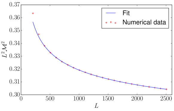
Figure 4: Scaling of matrix elements with system size $L$. The initial state contains one spinon with momentum $p=5.5$, while the final state contains three high-energy excitations with momenta $p_{p}=4.5,p_{p}=4.65,p_{h}=3.65$. The fit is to the functional form (80) with $a=0.42$, $b=5.6$, $c=0.044$. We have also considered additional excitations around the Fermi points in the final state as well as different momenta and found similar behaviour.

The situation is analogous to that for the dynamical structure factor [24, 25, 26, 27, 28, 29, 30, 31]. For the latter it was shown that in order to obtain finite results in the thermodynamic limit, an infinite summation over states that contain additional particle-hole pairs located at the “Fermi points” $\pm B$ was required. On the other hand, the result obtained by working at a fixed value of $L\approx 1000$ and not carrying out this summation was found to give an excellent approximation to the thermodynamic limit. We expect the decay rate to behave in an analogous way. In the following we determine the contributions of the 3-particle excitations described in section 3 to the decay rate for finite system sizes in the range $L\sim 500-1000$. We have verified that taking into account states with one additional particle-hole excitation gives only small corrections.

We now fix $L$ and then compute (77) for several values of the broadening $\eta$. The decay rates into the excitations considered in section 3 are shown in Figs 5(a), 5(b), 5(c) and 5(d).

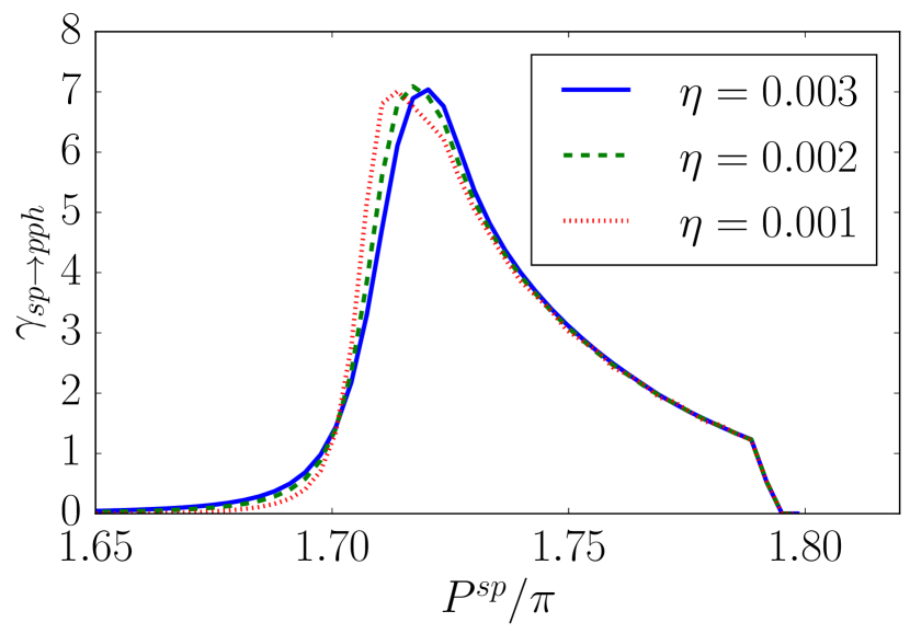
(a)

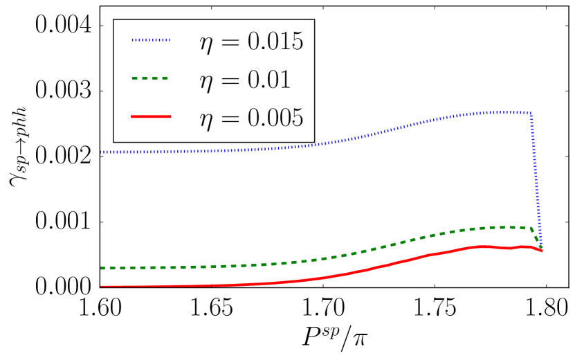
(b)

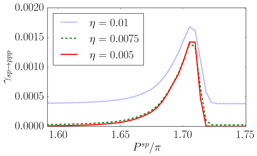
(c)

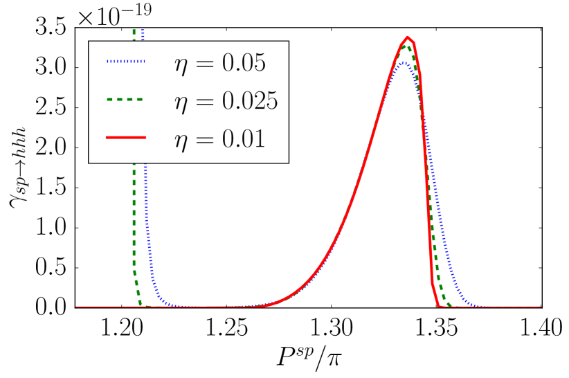
(d)

Figure 5: Coefficients of the decay rate for magnetization $m=3/10$ and several values of the broadening $\eta$ for (a) pph-type processes for $L=615$, (b) phh-type processes for $L=435$, (c) ppp-type processes for $L=455$, (d) hhh-type processes for $L=675$.

We see that the dominant decay channel for a one spinon excitation is decay into a 3-spinon excitation of pph type. We have argued above excitations involving higher numbers of particles should give smaller contributions to the decay rate. In order to check this assumption we have calculated the decay rate into a 5-spinon excitation of type ppphh, which we expect to provide the largest contribution among the 5-spinon excitations. The result is shown in Fig. 6(b). As expected the contribution is small. Moreover, it is mostly due to umklapp-type terms in the pph-channel, meaning particle-hole type excitations around the “Fermi sea” on top of the pph-type excitations (cf. Fig. 6(a)).

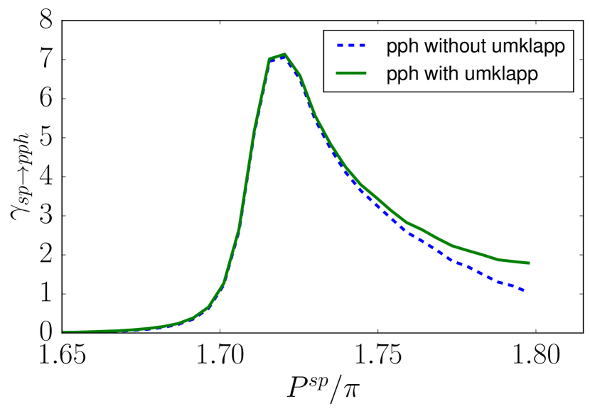
(a)

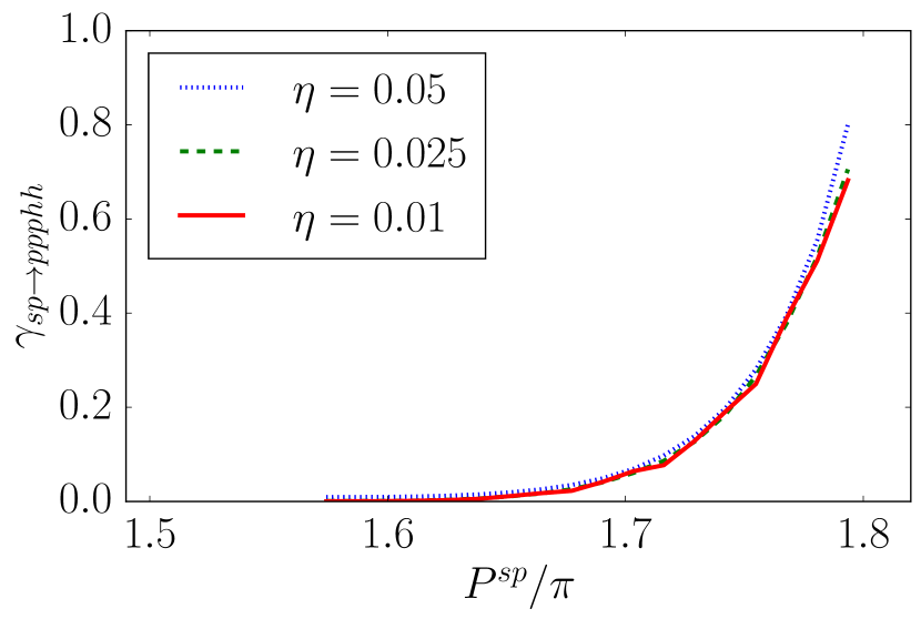
(b)

Figure 6: Coefficients of the decay rate for magnetization $m=3/10$ for (a) pph-type processes with and without umklapp terms for $\eta=0.002$ at $L=415$ and (b) ppphh-type processes for $L=155$ and several values of the broadening $\eta$.

It is clear from Fig. 5 that all other 3-spinon decay channels can be neglected compared to the pph one. Moreover, the decay rate coefficient is of order unity, which means that the decay rate itself is small and proportional to the square of the strength of the integrability breaking perturbation.

5.1 Extrapolation to $\eta=0$

The results of the previous section are for finite values of the system size and require a small, finite regularization parameter $\eta$. We will consider the extrapolation of these results to the thermodynamic limit and $\eta=0$. As we have seen above, the matrix elements of the perturbing operator scale as $L^{-1}$ up to corrections that decay algebraically with very small exponent or logarithmically, cf. Fig. 4. We expect that in order to take the thermodynamic limit, one would have to sum over an infinite number of particle-hole excitations at the Fermi points, in analogy with available results for the spin-spin correlation function [27, 28, 29, 30, 32]. Our situation is more complicated as we need to consider excited states with several elementary excitations at finite energies and summing over an infinite number of particle-hole excitations on top of these is beyond the scope of our work. However, we note that the main source of finite-size effects in our calculation is the necessity to have a sufficiently large value of the broadening $\eta$. This is required in order to obtain a good approximation to density of final states $\rho_{f}(E_{i})$. This imposes a restriction $\eta>\eta_{0}(L)={\rm const}/L$. Importantly, $\eta_{0}(L)$ tends to zero much faster than ${\cal M}^{2}L^{2}$. This allows us to extrapolate our results to $\eta=0$ as follows. We construct a smooth interpolation function $\mathcal{M}^{\text{cont}}_{pph}(p,z_{1}^{p},z_{2}^{p})$ for the matrix element multiplied by $L$, and then turn the sums over Bethe Ansatz (half-odd) integers into integrals using the Euler-Maclaurin sum formula. Taking the limit $\eta\to 0$ results in

$$\gamma^{\rm extra}_{\rm sp\rightarrow pph}(p) =\frac{1}{4\pi}\int_{D}\text{d}z_{1}^{p}\;\int_{D}\text{d}z_{2}^{p}\;\delta(\epsilon_{s}(z_{1}^{p})+\epsilon_{s}(z_{2}^{p})+\epsilon_{s}(z_{1}^{p}+z_{2}^{p}-p)-\varepsilon(p))$$

$$\hskip 56.9055pt\times\left|\mathcal{M}^{\text{cont}}_{pph}(p,z_{1}^{p},z_{2}^{p})\right|^{2}\ ,$$ (81)

where $D$ is the domain where the one-spinon exciation exists (the interval $[\pi/5,2\pi-\pi/5]$ for magnetization $m=3/10$). We stress again that we do not claim that this integral is the exact form one would get after summing all particle-hole pairs in the thermodynamic limit, but that the result of such a calculation is expected to be numerically very close to what is obtained here. One of the integrals can be carried out using the delta-function, which gives

$$\gamma^{\rm extra}_{\rm sp\rightarrow pph}(p) =\frac{1}{4\pi}\int_{D}\text{d}z_{1}^{p}\;\frac{\left|\mathcal{M}^{\text{cont}}_{pph}(p,z_{1}^{p},z)\right|^{2}}{\left|\varepsilon^{\prime}(z)+\varepsilon^{\prime}(z_{1}^{p}+z-p)\right|}\ ,$$ (82)

where $z$ is the solution of the equation $\epsilon_{s}(z_{1}^{p})+\epsilon_{s}(z)+\epsilon_{s}(z_{1}^{p}+z-p)-\varepsilon(p)=0$. Carrying out the remaining integral numerically leads to the result shown in Fig. 7

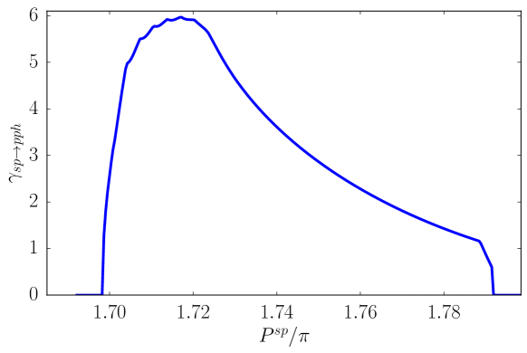
Figure 7: Decay rate to the pph-channel for $\eta\to 0$ at magnetization $m=3/10$. The wiggles are due to the finite size effects of the interpolated matrix element at $L=615$.

5.2 Density of kinematically allowed states and finiteness in the thermodynamic limit

A simpler quantity of interest is the density of final states to which transitions from the 1-spinon excitation are kinematically allowed. For free fermions this density of states exhibits a van Hove singularity that leads to logarithmic divergence at the threshold [33]. In the thermodynamic limit the pph channel density of kinematically relevant states is given by

$$\rho_{\text{pph}}(p) =\frac{1}{4\pi}\int_{D}\text{d}z_{1}^{p}\;\frac{1}{\left|\varepsilon^{\prime}(\tilde{z})+\varepsilon^{\prime}(z_{1}^{p}+z-p)\right|}$$ (83)

where $z$ is the same as in (82). Analogous expressions hold in the other channels. Results for the various possible types of 3-spinon final states are shown in Fig. 8. We see that densities of states are finite and do not display the kind of singularity encountered for free fermions.

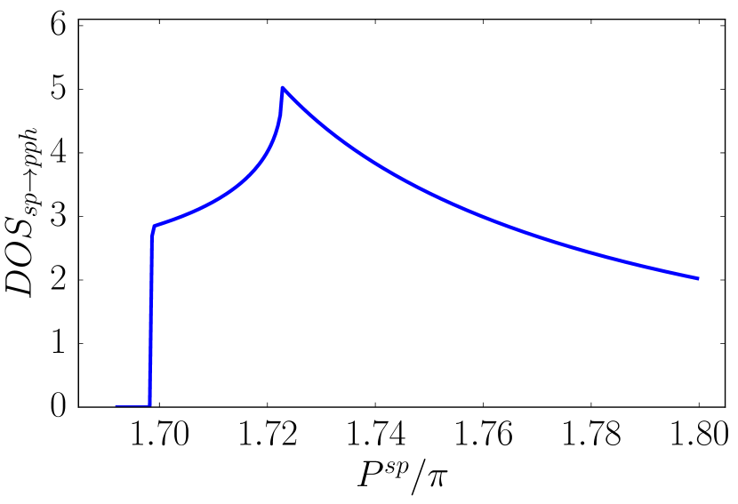
(a)

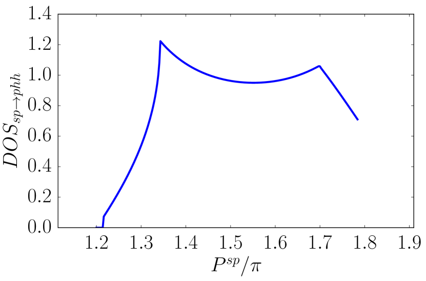
(b)

(c)

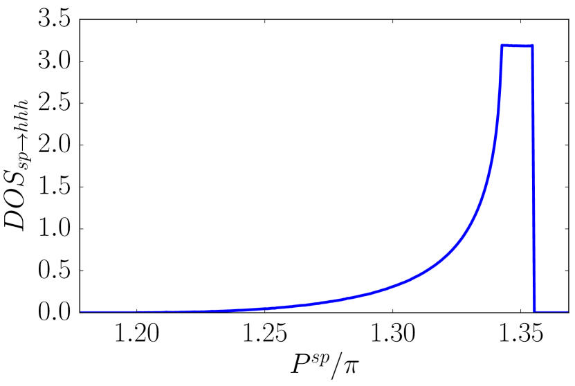
(d)

Figure 8: Density of states for the (a) pph-channel (b) phh-channel, (c) ppp-channel and (d) hhh-channel in the thermodynamic limit at magnetization $m=3/10$.

6 Conclusions

We have considered decay rates of the elementary spinon excitation in the spin-1/2 Heisenberg XXX model in a magnetic field perturbed by a weak integrability breaking interaction $\kappa\sum_{j}S_{j}^{z}S^{z}_{j+2}$. We have argued that the leading contribution arises from three spinon decay and have determined the corresponding rate. The latter is found to be small, indicating that spinons remain long-lived excitations in the non-integrable theory. Decay of elementary string excitations can be analyzed in an analogous fashion. This would be particularly interesting to do in the attractive regime $\Delta<0$ of the XXZ chain in a field, where they play an important role in the dynamics.

7 Acknowledgments

We are grateful to J.-S. Caux, L. Glazman and R. Pereira for helpful discussions. This work was supported by the EPSRC under grant EP/N01930X/1 and by the Clarendon Scholarship fund (SG).

Appendix A Matrix elements and suppression for non-highest weight states

We want to consider the normed matrix element of $\delta H$ between a highest weight state and a non-highest weight state

$$\frac{\left<\{\lambda\}\right|(S^{+})^{k}\sum_{j}S^{z}_{j}S^{z}_{j+2}\left|\{\mu\}\right>}{\sqrt{\left<\{\lambda\}\vphantom{\{\lambda\}}\right|(S^{+}S^{-})^{k}\left|\{\lambda\}\vphantom{\{\lambda\}}\right>}\sqrt{\left<\{\mu\}\ \vphantom{\{\mu\}}\right|\left.\{\mu\}\vphantom{\{\mu\}}\right>}}$$ (84)

where $\left<\{\lambda\}\right|$ and $\left|\{\mu\}\right>$ are highest weight Bethe ansatz states. We see immediately from the commutation relation

$$[S^{+},S^{z}_{j}]=-S^{+}_{j}$$ (85)

and from the relation for highest weight states $S^{+}\left|\{\mu\}\right>=0$ that for $k\geq 3$ the matrix element is exactly $0$. Furthermore inserting the cyclic shift operator (cf.[2]) $\;\text{exp}\left(i\hat{P}\right)$ and using

$$e^{-i\hat{P}}S_{j}^{a}e^{i\hat{P}}=S_{j+1}^{a}\quad a=z,+,-$$ (86)

and the fact that the highest weight states are eigenstates of the shift operator with eigenvalue $\;\text{exp}\left(iP_{\{\lambda\}}\right)$, where $P_{\{\lambda\}}$ is the momentum of the highest weight state, we obtain

$$\left<\{\lambda\}\right|e^{-i\hat{P}}e^{i\hat{P}} (S^{+})^{k}\sum_{j}S^{z}_{j}S^{z}_{j+2}\left|\{\mu\}\right>$$

$$=e^{i(P_{\{\lambda\}}-P_{\{\mu\}})}\left<\{\lambda\}\right|(S^{+})^{k}\sum_{j}S^{z}_{j}S^{z}_{j+2}\left|\{\mu\}\right>$$ (87)

and therefore we see that the momenta have to conincide. Using the commutation relation (85) we obtain for the normed matrix element for $k=1$ and $k=2$:

$$\frac{\left<\{\lambda\}\right|S^{+}\sum_{j}S^{z}_{j}S^{z}_{j+2}\left|\{\mu\}\right>}{\sqrt{\left<\{\mu\}\ \vphantom{\{\mu\}}\right|\left.\{\mu\}\vphantom{\{\mu\}}\right>\left<\{\lambda\}\vphantom{\{\lambda\}}\right|S^{+}S^{+}S^{-}S^{-}\left|\{\lambda\}\vphantom{\{\lambda\}}\right>}}$$

$$\qquad=\frac{1}{\sqrt{L-2(N-1)}}\frac{-\left<\{\lambda\}\right|\sum_{j}S^{+}_{j}S^{z}_{j+2}+S^{z}_{j}S^{+}_{j+2}\left|\{\mu\}\right>}{\sqrt{\left<\{\mu\}\ \vphantom{\{\mu\}}\right|\left.\{\mu\}\vphantom{\{\mu\}}\right>\left<\{\lambda\}\ \vphantom{\{\lambda\}}\right|\left.\{\lambda\}\vphantom{\{\lambda\}}\right>}}$$ (88)

$$\frac{\left<\{\lambda\}\right|(S^{+})^{2}\sum_{j}S^{z}_{j}S^{z}_{j+2}\left|\{\mu\}\right>}{\sqrt{\left<\{\mu\}\ \vphantom{\{\mu\}}\right|\left.\{\mu\}\vphantom{\{\mu\}}\right>\left<\{\lambda\}\vphantom{\{\lambda\}}\right|S^{+}S^{+}S^{-}S^{-}\left|\{\lambda\}\vphantom{\{\lambda\}}\right>}}$$

$$\qquad=\frac{1}{\sqrt{L-2(N-1)}\sqrt{L-2(N-2)}}\frac{2\left<\{\lambda\}\right|\sum_{j}S^{+}_{j}S^{+}_{j+2}\left|\{\mu\}\right>}{\sqrt{\left<\{\mu\}\ \vphantom{\{\mu\}}\right|\left.\{\mu\}\vphantom{\{\mu\}}\right>\left<\{\lambda\}\ \vphantom{\{\lambda\}}\right|\left.\{\lambda\}\vphantom{\{\lambda\}}\right>}}$$ (89)

We can now check numerically for solutions of the Bethe equation with same momenta using similar determinant expression as in (cf. B) for these matrix elements, that due to the normalization factor the matrix element is suppressed for large $L$ at finite magnetic field.

Appendix B Calculation of the next-nearest neighbor spin operator matrix element

We want to calculate the matrix element

$$\left<\{\lambda\}\right|\sigma_{j}^{z}\sigma^{z}_{j+2}\left|\{\mu\}\right>$$ (90)

with $\left|\{\mu\}\right>$, $\left|\{\mu\}\right>$ Bethe states and $\{\mu\}$, $\{\lambda\}$ satisfying the Bethe equations (12). We do the calculation for all $\Delta$. To obtain the formula for $\Delta=1$ the general functions $a$ and $d$ have to be replaced for the ones mentioned above and $\gamma$ has to be set to $1$ corresponding to the rescaling of $\{\lambda\}$ with $\gamma$ and taking the limit $\gamma\to 0$.

The $\sigma$ operators are given in terms of the Bethe-Ansatz operators $A,B,C,D$, as obtained in [21]:

$$\sigma_{j}^{z}=-2\prod_{i=1}^{j-1}(A+D)(\xi_{i})D(\xi_{j})\prod_{k=j+1}^{L}(A+D)(\xi_{k})+1$$ (91)

where $\xi_{i}$ is an inhomogeneity parameter, introduced at every site in the chain for technical reasons. We will set $\xi_{i}\to i\gamma/2$ in the end, but will keep them for the calculation. We note that now $d(\lambda)$ is defined as:

$$d(\lambda)=\prod_{l=1}^{L}b(\lambda-\xi_{l})$$ (92)

With this we can write the matrix element as:

$$\left<\{\lambda\}\right|\sigma_{j}^{z} \sigma^{z}_{j+2}\left|\{\mu\}\right>=\left<\{\lambda\}\right|\sigma_{j}^{z}\left|\{\mu\}\right>+\left<\{\lambda\}\right|\sigma_{j+2}^{z}\left|\{\mu\}\right>-\langle\{\lambda\}|\{\mu\}\rangle$$

$$+4\left<\{\lambda\}\right|\prod_{i=1}^{j-1}(A+D)(\xi_{i})D(\xi_{j})(A+D)(\xi_{j+1})D(\xi_{j+2})\prod_{k=j+3}^{L}(A+D)(\xi_{k})\left|\{\mu\}\right>$$ (93)

The maxtrix elements and the overlap in the first line are known [21, 20]. However as we are interested in $\sum_{j}\sigma_{j}^{z}\sigma_{j+2}^{z}$ and as $\left|\{\lambda\}\right>$ and $\left|\{\mu\}\right>$ are orthogonal and eigenstates of $\sigma^{z}$, we only need to calculate the expression in the second line. From the Yang-Baxter algebra one can derive the commutation relations between the operators $A,B,C,D$ and from this one gets ([12]):

$$A(\mu)\prod_{j=1}^{N}B(\lambda_{j})\left|0\right> =a(\mu)\prod_{j=1}^{N}b^{-1}(\lambda_{j}-\mu)\prod_{j=1}^{N}B(\lambda_{j})\left|0\right>$$

$$-\sum_{n=1}^{N}a(\lambda_{n})\frac{c(\lambda_{n}-\mu)}{b(\lambda_{n}-\mu)}\prod_{j\neq n}^{N}b^{-1}(\lambda_{j}-\lambda_{n})B(\mu)\prod_{j\neq n}^{N}B(\lambda_{j})\left|0\right>$$ (94)

$$D(\mu)\prod_{j=1}^{N}B(\lambda_{j})\left|0\right> =d(\mu)\prod_{j=1}^{N}b^{-1}(\mu-\lambda_{j})\prod_{j=1}^{N}B(\lambda_{j})\left|0\right>$$

$$-\sum_{n=1}^{N}d(\lambda_{n})\frac{c(\mu-\lambda_{n})}{b(\mu-\lambda_{n})}\prod_{j\neq n}^{N}b^{-1}(\lambda_{n}-\lambda_{j})B(\mu)\prod_{j\neq n}^{N}B(\lambda_{j})\left|0\right>$$ (95)

We furthermore know that

$$\prod_{i=1}^{j}(A+D)(\xi_{i})\left|\{\lambda\}\right>=\;\text{exp}\left(-ijP_{\{\lambda\}}\right)\left|\{\lambda\}\right>$$ (96)

where $\left|\{\lambda\}\right>$ is a Bethe state and $P_{\{\lambda\}}$ is the total momentum of $\left|\{\lambda\}\right>$ and

$$\prod_{i=1}^{L}(A+D)(\xi_{i})\left|\{\lambda\}\right>=1.$$ (97)

We now need to calculate the matrix element:

$$\mathcal{D}=\left<\{\lambda\}\right|D(\xi_{j})(A+D)(\xi_{j+1})D(\xi_{j+2})\left|\{\mu\}\right>$$ (98)

Using the commutation relations for $A,B,C,D$ (cf. [12]) we obtain:

$$\mathcal{D} =\text{I}+\text{II}$$ (99)

where I is dependent on simple matrix elements where two rapidities are replaced with inhomogeneities and II is dependent on a matrix element with three insertions of inhomogeneities:

$$\text{I}= \sum_{a=1}^{N}\frac{d(\mu_{a})c(\xi_{j+2}-\mu_{a})}{b(\xi_{j+2}-\mu_{a})}\prod_{i\neq a}^{N}\frac{1}{b(\mu_{a}-\mu_{i})}\Bigg{\{}\frac{1}{b(\xi_{j+2}-\xi_{j+1})}\prod_{i\neq a}^{N}\frac{1}{b(\mu_{i}-\xi_{j+1})}$$

$$\times\ \sum_{b\neq a}^{N}\frac{d(\mu_{b})c(\xi_{j}-\mu_{b})}{b(\xi_{j}-\mu_{b})b(\mu_{b}-\xi_{j+2})}\prod_{i\neq a,b}^{N}\frac{1}{b(\mu_{b}-\mu_{i})}\left<\{\lambda\}\right|B(\xi_{j})B(\xi_{j+2})\prod_{j\neq a,b}^{N}B(\mu_{j})\left|0\right>$$

$$+\frac{c(\xi_{j+1}-\xi_{j+2})}{b(\xi_{j+1}-\xi_{j+2})}\prod_{i\neq a}^{N}\frac{1}{b(\mu_{i}-\xi_{j+2})}\sum_{b\neq a}^{N}\frac{d(\mu_{b})c(\xi_{j}-\mu_{b})}{b(\xi_{j}-\mu_{b})}\frac{1}{b(\mu_{b}-\xi_{j+1})}$$

$$\times\prod_{i\neq a,b}^{N}\frac{1}{b(\mu_{b}-\mu_{i})}\left<\{\lambda\}\right|B(\xi_{j})B(\xi_{j+1})\prod_{j\neq a,b}^{N}B(\mu_{j})\left|0\right>\Bigg{\}}$$

$$\text{II}= \sum_{a=1}^{N}\frac{d(\mu_{a})c(\xi_{j+2}-\mu_{a})}{b(\xi_{j+2}-\mu_{a})}\prod_{i\neq a}^{N}\frac{1}{b(\mu_{a}-\mu_{i})}$$

$$\Bigg{\{}\sum_{b\neq a}^{N}\Bigg{[}\frac{c(\mu_{b}-\xi_{j+1})}{b(\mu_{b}-\xi_{j+1})}\prod_{i\neq a,b}^{N}\frac{1}{b(\mu_{i}-\mu_{b})}\frac{1}{b(\xi_{j+2}-\mu_{b})}$$

$$\hskip 85.35826pt+d(\mu_{b})\frac{c(\xi_{j+1}-\mu_{b})}{b(\xi_{j+1}-\mu_{b})b(\mu_{b}-\xi_{j+2})}\prod_{i\neq a,b}^{N}\frac{1}{b(\mu_{b}-\mu_{i})}\Bigg{]}$$

$$\hskip 28.45274pt\sum_{c\neq a,b}^{N}\frac{d(\mu_{c})c(\xi_{j}-\mu_{c})}{b(\xi_{j}-\mu_{c})b(\mu_{c}-\xi_{j+1})b(\mu_{c}-\xi_{j+2})}\prod_{i\neq a,b,c}^{N}\frac{1}{b(\mu_{c}-\mu_{i})}$$

$$\hskip 28.45274pt\left<\{\lambda\}\right|B(\xi_{j})B(\xi_{j+1})B(\xi_{j+2})\prod_{i\neq a,b,c}^{N}B(\mu_{i})\left|0\right>\Bigg{\}}$$ (100)

Now we can use Slavnov’s formula [20] for the overlap of two states. One of the states has to be a Bethe state, the other state can be parametrized by an arbitrary set of rapidities. Let $\{\lambda\}$ be solutions of the Bethe equations (12) and $\{\mu\}$ arbitrary, then one gets:

$$\langle\{\lambda\}|\{\mu\}\rangle=\frac{\text{det}\left(H(\{\lambda\},\{\mu\})\right)}{\prod_{j>k}\phi(\lambda_{k}-\lambda_{j})\prod_{j<k}\phi(\mu_{k}-\mu_{j})}$$ (101)

where $H$ is a matrix defined as

$$H_{ab}=\frac{\phi(i\gamma)}{\phi(\lambda_{a}-\mu_{b})}\left(a(\mu_{b})\prod_{k\neq a}\phi(\lambda_{k}-\mu_{b}+i\gamma)-d(\mu_{b})\prod_{k\neq a}\phi(\lambda_{k}-\mu_{b}-i\gamma)\right)$$ (102)

with $\phi(x)=x$ and $\gamma$ set to $1$ in the $\Delta=1$ scaling limit.

We will now treat I and II seperately.

B.1 Part II

For the part II, the limit of the $\xi_{j},\xi_{j+1}$ and $\xi_{j+2}$ can be taken seperately for the matrix element and the prefactor. Taking the limit $\xi_{i}\to i\gamma/2$ for the prefactor amounts to replacing the $\xi_{i}$ with $i\gamma/2$. For the matrix element we obtain using Slavnov’s determinant formula:

$$\left<\{\lambda\}\right|B(\xi_{j}) B(\xi_{j+1})B(\xi_{j+2})\prod_{i\neq k,m,n}B(\mu_{i})\left|0\right>=$$

$$\frac{\text{det}\left(H(\{\lambda\},\{\mu_{i\neq k,m,n},\xi_{j},\xi_{j+1},\xi_{j+2}\}\right)}{(\prod_{a>b}\phi(\lambda_{a}-\lambda_{b})\prod_{a<b}\phi(\mu_{b}-\mu_{a}))\big{|}_{\mu_{k}\to\xi_{j},\mu_{m}\to\xi_{j+1},\mu_{n}\to\xi_{j+2}}}$$ (103)

where

$$\prod_{a<b}\phi(\mu_{b}-\mu_{a}) \big{|}_{\mu_{k}\to\xi_{j},\mu_{m}\to\xi_{j+1},\mu_{n}\to\xi_{j+2}}=\frac{\phi(\xi_{j}-\xi_{j+1})\phi(\xi_{j}-\xi_{j+2})\phi(\xi_{j+1}-\xi_{j+2})}{\phi(\mu_{k}-\mu_{m})\phi(\mu_{k}-\mu_{n})\phi(\mu_{m}-\mu_{n})}$$

$$\hskip 28.45274pt\times\prod_{c\neq k,m,n}\frac{\phi(\xi_{j}-\mu_{c})\phi(\xi_{j+1}-\mu_{c})\phi(\xi_{j+2}-\mu_{c})}{\phi(\mu_{k}-\mu_{c})\phi(\mu_{m}-\mu_{c})\phi(\mu_{n}-\mu_{c})}\prod_{a<b}\phi(\mu_{b}-\mu_{a})$$ (104)

and in the determinant we have to replace $\mu_{k}\to\xi_{j},\mu_{m}\to\xi_{j+1}$ and $\mu_{n}\to\xi_{j+2}$. Therefore the important part when taking the limits is:

$$\lim_{\xi_{j},\xi_{j+2}\to i\gamma/2}\frac{\text{det}\left(H(\{\lambda\},\{\mu_{i\neq k,m,n},\xi_{j},i\gamma/2,\xi_{j+2}\}\right)}{\phi(\xi_{j}-i\gamma/2)\phi(\xi_{j}-\xi_{j+2})\phi(i\gamma/2-\xi_{j+2})}$$ (105)

where the limit $\xi_{j+1}\to i\gamma/2$ is already taken. Let us now take the limit $\xi_{j+2}\to i\gamma/2$. We see that both numerator and denominator go to zero here. Therefore using the rule of l’Hospital we obtain:

$$\lim_{\xi_{j},\xi_{j+2}\to i\gamma/2}\frac{\text{det}\left(H(\{\lambda\},\{\mu_{i\neq k,m,n},\xi_{j},i\gamma/2,\xi_{j+2}\}\right)}{\phi(\xi_{j}-i\gamma/2)\phi(\xi_{j}-\xi_{j+2})\phi(i\gamma/2-\xi_{j+2})}=$$

$$\qquad\lim_{\xi_{j}\to i\gamma/2}\frac{1}{\phi(\xi_{j}-i\gamma/2)\phi(\xi_{j}-i\gamma/2)}\lim_{x\to i\gamma/2}\frac{\text{d}}{\text{d}x}\text{det}\left(H(\{\lambda\},\{\mu_{i\neq k,m,n},\xi_{j},i\gamma/2,x\})\right)$$ (106)

Analogous to [34] we can now use a Laplace expansion of the determinant for the column that is dependent on $x$ and evaluate the derivative and limit:

$$\lim_{x\to i\gamma/2}\frac{\text{d}}{\text{d}x}\text{det}\left(H(\{\lambda\},\{\mu_{i\neq k,m,n},\xi_{j},i\gamma/2,x\})\right)=$$

$$\qquad=\lim_{x\to i\gamma/2}\frac{\text{d}}{\text{d}x}\sum_{i}(-1)^{(n+i)}C_{i}(x)\;\text{minor}_{ni}(H(\{\lambda\},\{\mu_{i\neq k,m,n},\xi_{j},i\gamma/2,x\}))$$

$$\qquad=\lim_{x\to i\gamma/2}\sum_{i}(-1)^{(n+i)}\left(\frac{\text{d}}{\text{d}x}C_{i}(x)\right)\;\text{minor}_{ni}(H(\{\lambda\},\{\mu_{i\neq k,m,n},\xi_{j},i\gamma/2,x\}))$$ (107)

where the minor is not dependent on $x$ and $C_{i}(x)$ is the $i$th element of the column $n$. Therefore we get:

$$\lim_{x\to i\gamma/2}\frac{\text{d}}{\text{d}x} \text{det}\left(H(\{\lambda\},\{\mu_{i\neq k,m,n},\xi_{j},i\gamma/2,x\})\right)=\text{det}\left(H_{1}(\{\lambda\},\{\mu\};m,n)\big{|}_{\mu_{k}\to\xi_{j}}\right)$$ (108)

with

$$(H_{1})_{ab}(\{\lambda\},\{\mu\};m,n) =\begin{cases}H_{ab}&b\neq m,n\\ \frac{\phi(i\gamma)}{\phi(\lambda_{a}-\frac{i\gamma}{2})\phi(\lambda_{a}+\frac{i\gamma}{2})}&b=m\\ \frac{\phi(i\gamma)\phi(2\lambda_{a})}{\phi(\lambda_{a}-\frac{i\gamma}{2})^{2}\phi(\lambda_{a}+\frac{i\gamma}{2})^{2}}&b=n\end{cases}$$ (109)

Repeating this step for the limit $\xi_{j}\to i\gamma/2$ using the rule of l’Hospital twice we finally obtain:

$$M_{ijk}^{(2)} \equiv\lim_{\xi_{j},\xi_{j+1},\xi_{j+2}\to i\gamma/2}\left<\{\lambda\}\right|B(\xi_{j})B(\xi_{j+1})B(\xi_{j+2})\prod_{i\neq k,m,n}B(\mu_{i})\left|0\right>$$

$$=\frac{1}{2}\prod_{i}\phi\left(\lambda_{i}+\frac{i\gamma}{2}\right)^{3}\phi(\mu_{m}-\mu_{n})\phi(\mu_{k}-\mu_{m})\phi(\mu_{k}-\mu_{n})$$

$$\quad\times\prod_{c\neq k,m,n}\frac{\phi(\mu_{c}-\mu_{k})\phi(\mu_{c}-\mu_{m})\phi(\mu_{c}-\mu_{n})}{\phi(\mu_{c}-\frac{i\gamma}{2})^{3}}$$

$$\quad\times\frac{\text{det}\left(H_{2}\right)}{\prod_{a>b}\phi(\lambda_{b}-\lambda_{a})\prod_{a<b}\phi(\mu_{b}-\mu_{a})}$$ (110)

where

$$(H_{2})_{ab}(\{\lambda\},\{\mu\};k,m,n) =\begin{cases}H_{ab}&b\neq m,n,k\\ \frac{\phi(i\gamma)}{\phi(\lambda_{a}-\frac{i\gamma}{2})\phi(\lambda_{a}+\frac{i\gamma}{2})}&b=m\\ \frac{\phi(i\gamma)\phi(2\lambda_{a})}{\phi(\lambda_{a}-\frac{i\gamma}{2})^{2}\phi(\lambda_{a}+\frac{i\gamma}{2})^{2}}&b=n\\ \frac{\partial^{2}}{\partial x^{2}}\left(\frac{\phi(i\gamma)}{\phi(\lambda_{a}-x)\phi(\lambda_{a}-x+i\gamma)}\right)\big{|}_{x=\frac{i\gamma}{2}}&b=k\end{cases}$$ (111)

With this we obtain after some algebra:

II $$=-\frac{1}{2}\frac{\prod_{k}\phi(\lambda_{k}+i\gamma/2)^{3}\phi(\mu_{k}-i\gamma/2)^{-3}}{\prod_{a>b}\phi(\lambda_{b}-\lambda_{a})\prod_{a<b}\phi(\mu_{b}-\mu_{a})}\sum_{n=1}^{N}d(\mu_{n})\phi(\mu_{n}-i\gamma/2)\prod_{i}\phi(\mu_{i}-\mu_{n}-i\gamma)$$

$$\quad\sum_{m\neq n}\prod_{i}\phi(\mu_{i}-\mu_{m}+i\gamma)\phi(\mu_{m}-i\gamma/2)\left[\frac{\phi(\mu_{m}-3i\gamma/2)}{\phi(\mu_{m}-\mu_{n}-i\gamma)}-\frac{\phi(\mu_{m}+i\gamma/2)}{\phi(\mu_{m}-\mu_{m}+i\gamma)}\right]$$

$$\quad\sum_{k\neq m,n}d(\mu_{k})\prod_{i}\phi(\mu_{i}-\mu_{k}-i\gamma)\frac{\phi(\mu_{k}+i\gamma/2)^{2}}{\phi(\mu_{m}-\mu_{k}-i\gamma)\phi(\mu_{n}-\mu_{k}-i\gamma)}$$

$$\hskip 85.35826pt\times\text{det}\left(H_{2}(\{\lambda\},\{\mu\};k,m,n)\right)$$ (112)

Using a Lemma from Laplace’s determinant formula ([23]) we finally obtain:

II $$=-\frac{1}{2}\frac{\prod_{k}\phi(\lambda_{k}+i\gamma/2)^{3}\phi(\mu_{k}-i\gamma/2)^{-3}}{\prod_{a>b}\phi(\lambda_{b}-\lambda_{a})\prod_{a<b}\phi(\mu_{b}-\mu_{a})}$$

$$\qquad\times\sum_{n=1}^{N}\sum_{m\neq n}A_{nm}\left[\text{det}\left(G_{nm}+B_{nm}\right)-\text{det}\left(G_{nm}\right)\right]$$ (113)

with

$$(G_{nm})_{ab} =\begin{cases}H_{ab}&b\neq m,n\\ \frac{\phi(i\gamma)\phi(2\lambda_{a})}{\phi(\lambda_{a}-\frac{i\gamma}{2})^{2}\phi(\lambda_{a}+\frac{i\gamma}{2})^{2}}&b=m\\ \frac{\partial^{2}}{\partial x^{2}}\left(\frac{\phi(i\gamma)}{\phi(\lambda_{a}-x)\phi(\lambda_{a}-x+i\gamma)}\right)\big{|}_{x=\frac{i\gamma}{2}}&b=n\end{cases}$$ (114)

$$(B_{nm})_{ab} =(1-\delta_{bm})(1-\delta_{bn})d(\mu_{b})$$

$$\hskip 28.45274pt\prod_{i\neq m,n}\phi(\mu_{i}-\mu_{b}-i\gamma)\phi(\mu_{b}+i\gamma/2)^{2}\frac{\phi(i\gamma)}{\phi(\lambda_{a}-i\gamma/2)\phi(\lambda_{a}+i\gamma/2)}$$ (115)

B.2 Part I

First we can take the limit $\xi_{j},\xi_{j+2}\to i\gamma/2$. This again just amounts to replacing the $\xi_{j}$ and $\xi_{j+2}$ with $i\gamma/2$ in the prefactors and doing a similar analysis for the matrix element depending on both $\xi_{j}$ and $\xi_{j+2}$ as for the part II. However performing the limit $\xi_{j+1}\to i\gamma/2$ is a bit more involved, as the limit can not be taken independently for prefactor and matrix elements. This is due to terms $\propto\frac{1}{\xi_{j+1}-i\gamma/2}$ appearing in the prefactors. Doing a consistent series expansion in $\xi_{j+1}-i\gamma/2$ again utilizing the Laplace determinant expansion and then taking the limit $\xi_{j+1}\to i\gamma/2$ we obtain after some calculation:

I $$=-\phi(i\gamma)\frac{\prod_{k}\phi(\lambda_{k}+i\gamma/2)^{2}\phi(\mu_{k}+i\gamma/2)\phi(\mu_{k}-i\gamma/2)^{-3}}{\prod_{a>b}\phi(\lambda_{b}-\lambda_{a})\prod_{b>a}\phi(\mu_{b}-\mu_{a})}$$

$$\left\{\sum_{n=1}^{N}d(\mu_{n})\prod_{i}\phi(\mu_{i}-\mu_{n}-i\gamma)\frac{\phi(\mu_{n}-i\gamma/2)^{2}}{\phi(\mu_{n}+i\gamma/2)}\right.$$

$$\times\left[\sum_{m\neq n}d(\mu_{m})\prod_{i\neq n}\phi(\mu_{i}-\mu_{m}-i\gamma)\phi(\mu_{m}+i\gamma/2)\right.$$

$$\left(\frac{\phi^{\prime}(i\gamma)}{\phi(i\gamma)}-\sum_{d\neq n}\frac{\phi(i\gamma)}{\phi(\mu_{d}-i\gamma/2)\phi(\mu_{d}+i\gamma/2)}+\sum_{d\neq m,n}\frac{\phi^{\prime}(\mu_{d}-i\gamma/2)}{\phi(\mu_{d}-i\gamma/2)}\right.$$

$$-\sum_{b}\frac{\phi^{\prime}(\lambda_{b}+i\gamma/2)}{\phi(\lambda_{b}+i\gamma/2)}+\left.\frac{\phi(i\gamma)}{\phi(\mu_{m}+i\gamma/2)\phi(\mu_{m}-i\gamma/2)}\right)\text{det}\left(H_{3}(\{\lambda\},\{\mu\};m,n)\right)+$$

$$\left.\left.\sum_{m\neq n}d(\mu_{m})\phi(\mu_{m}+i\gamma/2)\prod_{i\neq n}\phi(\mu_{i}-\mu_{m}-i\gamma)\frac{1}{2}\text{det}\left(H_{4}(\{\lambda\},\{\mu\};m,n)\right)\right]\right\}$$ (116)

with

$$(H_{3})_{ab} =\begin{cases}H_{ab}&b\neq m,n\\ \frac{\phi(i\gamma)}{\phi(\lambda_{a}+i\gamma/2)\phi(\lambda_{a}-i\gamma/2)}&b=m\\ \frac{\phi(i\gamma)\phi(2\lambda_{a})}{\phi(\lambda_{a}-\frac{i\gamma}{2})^{2}\phi(\lambda_{a}+\frac{i\gamma}{2})^{2}}&b=n\end{cases}$$ (117)

$$(H_{4})_{ab} =\begin{cases}H_{ab}&b\neq m,n\\ \frac{\phi(i\gamma)}{\phi(\lambda_{a}+i\gamma/2)\phi(\lambda_{a}-i\gamma/2)}&b=m\\ \frac{\partial^{2}}{\partial x^{2}}\left(\frac{\phi(i\gamma)}{\phi(\lambda_{a}-x)\phi(\lambda_{a}-x+i\gamma)}\right)\big{|}_{x=\frac{i\gamma}{2}}&b=n\end{cases}$$ (118)

using the Lemma from Laplace’s determinant formula again, we finally obtain:

I $$=-\phi(i\gamma)\frac{\prod_{k}\phi(\lambda_{k}+i\gamma/2)^{2}\phi(\mu_{k}+i\gamma/2)\phi(\mu_{k}-i\gamma/2)^{-3}}{\prod_{a>b}\phi(\lambda_{b}-\lambda_{a})\prod_{b>a}\phi(\mu_{b}-\mu_{a})}$$

$$\quad\times\sum_{n}A_{n}\Big{(}\text{det}\left(G_{n}^{(1)}+B_{n}^{(1)}\right)+\text{det}\left(G_{n}^{(2)}+B_{n}^{(2)}\right)$$

$$\qquad\qquad\qquad-\text{det}\left(G^{(1)}\right)-\text{det}\left(G^{(2)}\right)\Big{)}$$ (119)

where

$$(G^{(1)}_{n})_{ab} =\begin{cases}H_{ab}&b\neq n\\ \frac{\phi(i\gamma)\phi(2\lambda_{a})}{\phi(\lambda_{a}-\frac{i\gamma}{2})^{2}\phi(\lambda_{a}+\frac{i\gamma}{2})^{2}}&b=n\end{cases}$$ (120)

$$(G^{(2)}_{n})_{ab} =\begin{cases}H_{ab}&b\neq n\\ \frac{\partial^{2}}{\partial x^{2}}\left(\frac{\phi(i\gamma)}{\phi(\lambda_{a}-x)\phi(\lambda_{a}-x+i\gamma)}\right)\big{|}_{x=\frac{i\gamma}{2}}&b=n\end{cases}$$ (121)

$$(B^{(1)}_{n})_{ab} =(1-\delta_{bn})d(\mu_{b})\prod_{i\neq n}\phi(\mu_{i}-\mu_{b}+i\gamma)\phi(\mu_{b}+i\gamma/2)$$

$$\left(\frac{\phi^{\prime}(i\gamma)}{\phi(i\gamma)}-\sum_{d\neq n}\frac{\phi(i\gamma)}{\phi(\mu_{d}-i\gamma/2)\phi(\mu_{d}+i\gamma/2)}+\sum_{d\neq m,n}\frac{\phi^{\prime}(\mu_{d}-i\gamma/2)}{\phi(\mu_{d}-i\gamma/2)}\right.$$

$$\left.-\sum_{b}\frac{\phi^{\prime}(\lambda_{b}+i\gamma/2)}{\phi(\lambda_{b}+i\gamma/2)}+\frac{\phi(i\gamma)}{\phi(\mu_{m}+i\gamma/2)\phi(\mu_{m}-i\gamma/2)}\right)$$ (122)

$$(B^{(2)}_{n})_{ab} =(1-\delta_{bn})\frac{1}{2}d_{\mu_{b}}$$

$$\hskip 28.45274pt\times\prod_{i\neq n}\phi(\mu_{i}-\mu_{b}-i\gamma)\phi(\mu_{b}+i\gamma)\frac{\phi(i\gamma)}{\phi(\lambda_{a}+i\gamma/2)\phi(\lambda_{a}-i\gamma/2)}$$ (123)

B.3 Total matrix element

We can now put together the total matrix element. We obtain

$$\sum_{j}\left<\{\lambda\}\right|S_{j}^{z}S_{j+2}^{z}\left|\{\mu\}\right> =e^{iP_{\{\lambda\}}+2iP_{\{\mu\}}}\sum_{j}e^{-ij(P_{\{\lambda\}}-P_{\{\mu\}})}\mathcal{D}$$ (124)

$$=Le^{iP_{\{\lambda\}}+2iP_{\{\mu\}}}\delta_{P_{\{\lambda\}},P_{\{\mu\}}}\mathcal{D}$$ (125)

References

- [1] L. D. Faddeev, L. A. Takhtajan, What is the spin of a spin wave?, Lett. A 85 375 (1981)
- [2] L.D. Faddeev and L. Takhtajan, Spectrum and scattering of excitations in the one-dimensional isotropic Heisenberg model, J. Sov. Math. 24, 241 (1984).
- [3] G. Delfino, G. Mussardo, P. Simonetti, Non-integrable quantum field theories as perturbations of certain integrable models, Nucl. Phys. B473, 469 (1996).
- [4] G. Delfino, G. Mussardo, Non-integrable aspects of the multi-frequency sine-Gordon model, Nucl. Phys. B516, 675 (1998).
- [5] G. Delfino, P. Grinza, G. Mussardo, Decay of particles above threshold in the Ising field theory with magnetic field, Nucl. Phys. B737, 291 (2006).
- [6] B. Pozsgay and G. Takacs, Characterization of resonances using finite size effects, Nucl. Phys. B 748, 485 (2006).
- [7] A. Imambekov, T. L. Schmidt, and L. I. Glazman, One-dimensional quantum liquids: Beyond the Luttinger liquid paradigm, Rev. Mod. Phys. 84, 1253 (2012); R. G. Pereira, S. R. White, and I. Affleck, Spectral function of spinless fermions on a one-dimensional lattice, Phys. Rev. B79, 165113 (2009) and references therein.
- [8] F.H.L. Essler, R.G. Pereira and I. Schneider, Spin-charge-separated quasiparticles in one-dimensional quantum fluids, Phys. Rev. B91, 245150 (2015).
- [9] T.L. Schmidt, A. Imambekov, and L. I. Glazman, Spin-charge separation in one-dimensional fermion systems beyond Luttinger liquid theory, Phys. Rev. B 82 245104 (2010); F.H.L. Essler, Threshold singularities in the one-dimensional Hubbard model, Phys. Rev. B 81, 205120 (2010).
- [10] F. H. L. Essler, H. Frahm, F. Göhmann, A. Klümper, and V. E. Korepin, The One-Dimensional Hubbard Model, Cambridge University Press, Cambridge (2005).
- [11] M. Takahashi, Thermodynamics of One-Dimensional Solvable Models, Cambridge University Press (1999)
- [12] V. Korepin, N. Bogoliubov, and A. Izergin, Quantum Inverse Scattering Method and Correlation Functions, Cambridge Monographs on Mathematical Physics, Cambridge University Press (1997)
- [13] M. Peskin, D. Schroeder, An introduction to quantum field theory, Westview Press Reading (Mass.) (1995)
- [14] H. Bethe, Zur Theorie der Metalle. I. Eigenwerte und Eigenfunktionen der linearen Atomkette, Zeitschrift für Physik, 71 205-226 (1931)
- [15] M. Gaudin, J.S. Caux, The Bethe Wavefunction, Cambridge University Press (2014)
- [16] R. Orbach, Linear Antiferromagnetic Chain with Anisotropic Coupling, Phys. Rev. 112, 309 (1958)
- [17] G. Mussardo, Statistical field theory an introduction to exactly solved models in statistical physics, Oxford University Press (2010)
- [18] M. Gaudin, B. M. McCoy, T. T. Wu, Normalization sum for the Bethe’s hypothesis wave functions of the Heisenberg-Ising chain, Phys. Rev. D 23, 417 (1981)
- [19] V. E. Korepin, Calculation of norms of Bethe wave functions, Comm. Math. Phys. 86, 391 (1982)
- [20] N. A. Slavnov, Calculation of scalar products of wave functions and form factors in the framework of the algebraic Bethe ansatz, Teor. Mat. Fiz. 79, 232 (1989)
- [21] N. Kitanine, J. M. Maillet, V. Terras, Form factors of the XXZ Heisenberg spin-1/2 finite chain, Nucl. Phys. B 554, 647 (1999)
- [22] N. Kitanine, J. M. Maillet, V. Terras, Correlation functions of the XXZ Heisenberg spin-1/2 chain in a magnetic field, Nucl. Phys. B 567, 554 (2000)
- [23] A. Klauser, J. Mossel, J. S. Caux, Adjacent spin operator dynamical structure factor of the S = 1/2 Heisenberg chain, J. Stat. Mech. P03012 (2012)
- [24] J. S. Caux, Correlation functions of integrable models: A description of the ABACUS algorithm, Journal of Mathematical Physics 50, 095214 (2016)
- [25] R. G. Pereira, J. Sirker, J. S. Caux, R. Hagemans, J. M. Maillet, S. R. White, I. Affleck, Dynamical structure factor at small q for the XXZ spin-1/2 chain, J. Stat. Mech. P08022 (2007)
- [26] J. S. Caux, R. Hagemans, J. M. Maillet, Computation of dynamical correlation functions of Heisenberg chains: the gapless anisotropic regime, J. Stat. Mech. P09003 (2005)
- [27] A. Shashi, L. I. Glazman, J. S. Caux, A. Imambekov, Nonuniversal prefactors in the correlation functions of one-dimensional quantum liquids, Phys. Rev. B 84, 045408 (2011)
- [28] A. Shashi, M. Panfil, J. S. Caux, A. Imambekov, Exact prefactors in static and dynamic correlation functions of one-dimensional quantum integrable models: Applications to the Calogero-Sutherland, Lieb-Liniger, and XXZ models, Phys. Rev. B 85, 155136 (2012)
- [29] N. Kitanine, K. K. Kozlowski, J. M. Maillet, N. A. Slavnov, V. Terras, On the thermodynamic limit of form factors in the massless XXZ Heisenberg chain, J. Math. Phys. 50 095209 (2009)
- [30] N. Kitanine, K. K. Kozlowski, J. M. Maillet, N. A. Slavnov, V. Terras, Thermodynamic limit of particle-hole form factors in the masless XXZ Heisenberg chain, J. Stat. Mech. 05 P05028 (2011)
- [31] N. Kitanine, K. K. Kozlowski, J. M. Maillet, N. A. Slavnov, V. Terras, Form factor approach to dynamical correlation functions in critical models, J. Stat. Mech., P09001 (2012)
- [32] N. Kitanine, K. K. Kozlowski, J. M. Maillet, N. A. Slavnov, V. Terras, A form factor approach to the asymptotic behavior of correlation functions in critical models, J. Stat. Mech. : Th. and Exp., P12010 (2011)
- [33] R. G. Pereira, S. R. White, I. Affleck, Spectral function of spinless fermions on a one-dimensional lattice, Phys. Rev. B 79 165113 (2009)
- [34] R. L. Hagemans, Dynamics of Heisenberg Spin Chains, PhD thesis (2007), retrieved from UvA-DARE database, uvapub:52466