Scene Recognition by Combining Local and Global Image Descriptors

Abstract

Object recognition is an important problem in computer vision, having diverse applications. In this work, we construct an end-to-end scene recognition pipeline consisting of feature extraction, encoding, pooling and classification. Our approach simultaneously utilize global feature descriptors as well as local feature descriptors from images, to form a hybrid feature descriptor corresponding to each image. We utilize DAISY features associated with key points within images as our local feature descriptor and histogram of oriented gradients (HOG) corresponding to an entire image as a global descriptor. We make use of a bag-of-visual-words encoding and apply Mini-Batch K-Means algorithm to reduce the complexity of our feature encoding scheme. A 2-level pooling procedure is used to combine DAISY and HOG features corresponding to each image. Finally, we experiment with a multi-class SVM classifier with several kernels, in a cross-validation setting, and tabulate our results on the fifteen scene categories dataset. The average accuracy of our model was 76.4% in the case of a 40%–60% random split of images into training and testing datasets respectively. The primary objective of this work is to clearly outline the practical implementation of a basic screne-recognition pipeline having a reasonable accuracy, in python, using open-source libraries. A full implementation of the proposed model is available in our github repository.

I Introduction

Object recognition is an interesting computer vision problem with diverse applications in a variety of fields such as automated surveillance, robotics, human computer interaction, video indexing and vehicle navigation [1]. In this work, we build an end-to-end pipeline for recognizing natural scene categories in python and report our results on the fifteen scene categories dataset [2]. Our pipeline essentially consists of feature extraction, encoding, pooling and classification steps. However, we augment this standard pipeline by coming up with a hybrid feature descriptor that simultaneously make use of local feature descriptors as well as global feature descriptors at a different granularity, with the objective of improving the classification accuracy. We also reduce the time-complexity of our encoding step by using Mini-Batch K-Means algorithm instead of the standard K-means algorithm, for constructing the bag of visual words, since the number of feature descriptors involved would be quite large in practice. In our experiments with the fifteen scene categories dataset, the number of feature descriptors extracted from the training data set were around 1.9 million. We utilize a 2-level pooling scheme to combine DAISY and HOG features corresponding to each image. We train a multi-class SVM classifier with multiple kernel choices in a cross-validation setting and tabulate our classification results.

We describe each of the steps in our pipeline in detail in Section II and also present our design choices and their contributions in improving the overall performance of our scene recognition pipeline. In Section III, we study the impact of the vocabulary size in our encoding step and the effects of various kernel choices as well as parameters, and present our results. We discuss the key insights in the light of our results in Section IV. Section V concludes our paper.

II Methodology

Our scene recognition pipeline involves feature extraction, encoding, pooling and classification steps. Our model has multiple tunable parameters such as size of the visual vocabulary ($K$), the kernel to be used by the SVM classifier (e.g. linear vs. Gaussian) as well as SVM hyper-parameters such as $C$ and $\gamma$. We make use of cross-validation to empirically choose the optimal hyper-parameters. We discover the optimal $K$ empirically for a linear SVM first. We use this $K$ and further perform a grid-search to discover the optimal $C$ and $\gamma$ corresponding to an SVM model having a Radial Basis Function(RBF) kernel. Details of each of our pipeline steps are presented below.

II-A Feature Extraction

From each image, we first extract DAISY[3] features corresponding to the key-points detected from the image. We make use of the skimage library (scikit–image) [4] for feature extraction. Corresponding to each keypoint in the image, we extract a DAISY descriptor. We also extract a standard HOG descriptor corresponding to the whole image at a different granularity (by making use of the parameters pixels_per_cell, cells_per_block and orientations), effectively allowing us to choose features at different scales. We make use of the DAISY descriptors extracted from all the training images to form a bag-of-visual-words by clustering them using Mini-Batch K-Means. We empirically determine the best visual vocabulary size ($K$) through cross-validation.

II-B Encoding

We make use of the local DAISY features corresponding to each keypoints to encode each image as a histogram of visual words. We use the standard “bag-of-visual-words” concept here. Concretely, we apply K-means algorithm to quantize DAISY features into ‘$K$’ clusters to form “visual words” in a vocabulary. $K$ represents the vocabulary size. Corresponding to each image, we form a histogram with ‘$K$’ as the dimensionality, by using this vocabulary. This encoded representation of the image forms the “DAISY histogram” and constitutes a portion of our hybrid feature descriptor.

II-C Pooling

We make use of a 2 level pooling scheme in our scene recognition pipeline. From the DAISY features, we construct a histogram by representing frequency of each visual word in each image. We perform this by selecting each key point in the image and looking up the cluster id corresponding to that DAISY descriptor and incrementing the count corresponding to that bin in our “DAISY histogram”. This procedure is effectively a “sum pooling”. We do an L2 normalization of the resulting histogram to form a DAISY histogram feature which we call as “DAISY histogram”. For the 2nd level pooling, we take the HOG global descriptor corresponding to each image and do an L2 normalization followed by a concatenation with the corresponding DAISY histogram feature, to form our hybrid feature descriptor.

II-D Classification

We make use of the standard SVM classifier with various kernels, for classification. We utilize the sklearn library (sckit-learn) [5] for the SVM implementations. We perform crossvalidation by randomly splitting the dataset into a training and validation set. We build the “visual vocabulary” as well as training feature vectors from the training split. We report the overall accuracy, confusion-matrix as well as standard information-retrieval statistics such as precision, recall and f-measure corresponding to our experiments.

III Results

We conducted our experiments on a standard DELL Precision Tower 5810 workstation, running 64 bit ubuntu 14.04 LTS. Once the execution pipeline described in Section II was built, the optimal size of visual vocabulary ($K$) was emperically discovered, by running the pipeline 3 times corresponding to each $K$ and averaging their accuracy. A linear SVM model was used for classification. The optimal value of $K$ was found to be 600 and the average accuracy across 3 runs was 73.14%. The results are summarized in Table I and plotted in the Figure 1

TABLE I: Average accuracy of MiniBatch K-Means for different $K$

K	Accuracy(%)
100	70.2628
200	70.3092
300	72.0269
400	71.7948
500	72.6769
600	73.1411
700	72.7233
800	71.6091
900	70.5413
1000	70.1697

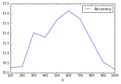
Figure 1: Plot between $K$ and Accuracy(Linear SVM)

After obtaining the optimal $K$ using a linear SVM, we changed the kernel to RBF and performed a grid search for discovering the optimal $C$ and $\gamma$ by varying log($C$) within the interval [-3 3] and log($\gamma$) within the interval [-3 2] with the value of $K$ as 600. The optimal value of log($C$) was 1.679 and log($\gamma$) was -0.163 for an accuracy of 74.5%. The optimization response surface is plotted in Figure 2.

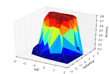
Figure 2: RBF kernel optimization response surface

We executed the pipeline with an RBF kernel for optimal $K$, $C$ and $\gamma$, and the final accuracy was found to be 76.4%. The average precision is 77%, average recall is 76% and average f1-score is 76%. The confusion matrix for the model is depicted in figure 3. The pipeline with a linear kernel and optimal $K$ reported an accuracy of 75.6%, average precision of 76%, average recall of 76% and average f1-score of 75%. This shows that kernelizing SVM marginally improves the accuracy. The confusion matrix for the classifier is shown in Figure 4.

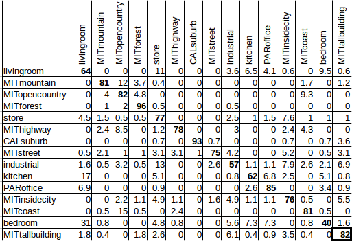
Figure 3: Confusion Matrix: SVM with hybrid feature and RBF Kernel (60% Test data)

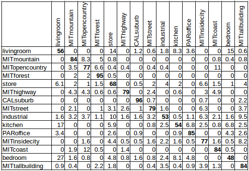
Figure 4: Confusion Matrix: SVM with hybrid features and linear Kernel (60% Test data)

We observed that executing the pipeline(linear SVM) with HOG descriptors alone is providing an accuracy of 59.1%, average precision of 59%, average recall is 59% and average f1-score is 58%. With DAISY descriptors alone, the accuracy was 70.8%, average precision was 70%, average recall was 71% and average f1-score was 70%. The confusion matrix corresponding the model with HOG features alone and the model with DAISY features alone are shown in Figures 5 and 6 respectively.

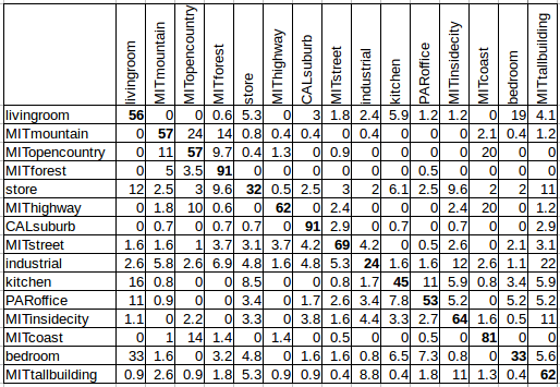
Figure 5: Confusion Matrix: SVM with HOG feature alone and RBF Kernel (60% Test data)

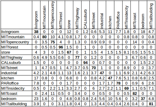
Figure 6: Confusion Matrix: SVM with DAISY features alone and linear Kernel (60% Test data)

We observe that there is a significant increase in the model accuracy while employing a hybrid feature descriptor comprising of HOG and DAISY descriptors, compared to models that utilize either HOG features or DAISY features only.

IV Discussion

We observe in section III that by utilizing a hybrid feature descriptor, our model accuracy is significantly improved. The relatively poor performance of models utilizing HOG descriptors alone can be attributed to its inability to deal with scale, orientation or translation. However, HOG descriptors can be combined with a dense feature descriptors such as DAISY which are capable of dealing with scale, orientation and translation, to produce superior results. The two-level pooling scheme used by our model improves the overall results. L2 normalization is performed on the DAISY and HOG descriptors to bring both these components to scale, so that their concatenation would result in a meaningful feature descriptor. We also used an approximation technique while building the bag-of-visual-words representation, to reduce the algorithmic complexity involved in this process. In our experiments, the number of DAISY descriptors extracted from the training dataset was around 1.9 million. The scikit-learn K-Means implementation ran for several hours to produce a reasonable clustering. We made use of the Mini-Batch K-means proposed by David Sculley in his paper titled “Web-scale k-means clustering” [6]. Execution time for the Mini-Batch K-means implementation in scikit-learn on the same dataset was around 45 seconds for K=600. The running time of Mini-Batch K-Means against different values of $K$ is summarized in Table II

TABLE II: Average execution time taken by MiniBatch K-Means for different values of $K$

K	Time(seconds)
100	7.898881
200	12.972909
300	17.126809
400	20.611251
500	23.639403
600	45.750178
700	33.864268
800	55.053441
900	74.374957
1000	52.925832

Some of the images misclassified by our model are shown in Figures 7, 8, 9, 10, 11 and 12. It is interesting to note that some of these images may be prone to misclassification even for a human being.

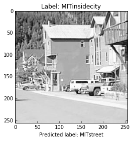
Figure 7: Sample misclassified image 1

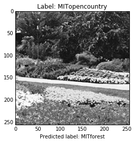
Figure 8: Sample misclassified image 2

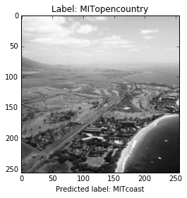
Figure 9: Sample misclassified image 3

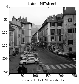
Figure 10: Sample misclassified image 4

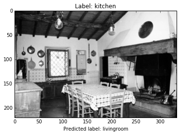
Figure 11: Sample misclassified image 5

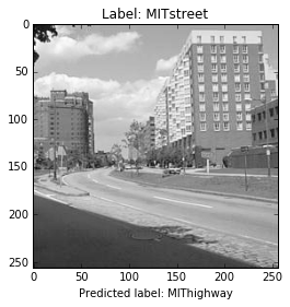
Figure 12: Sample misclassified image 6

V Conclusion

We implemented an end-to-end scene recognition pipeline consisting of feature extraction, encoding, pooling and classification steps using open-source libraries in python. We simultaneously utilized global feature descriptors as well as local feature descriptors from images, to form a hybrid feature descriptor for each image. DAISY descriptors associated with key points in images were utilized as local feature descriptor and HOG feature (at a different granularity) corresponding to an entire image was used as a global feature descriptor. We made use of a bag of visual words encoding and applied Mini-Batch K-Means algorithm to significantly reduce the complexity of our encoding scheme. A 2-level pooling scheme was used to combine DAISY and HOG features corresponding to each image. Finally, a multi-class SVM classifier was trained with multiple kernel choices in a cross-validation setting to evaluate our model perfomance. The overall accuracy of our hybrid model was 76.4% which was better than the accuracies of models that made use of HOG or DAISY features alone. A full implementation of the proposed model is available in our github repository[7].

References

- [1] A. Yilmaz, O. Javed, and M. Shah, “Object tracking: A survey,” Acm computing surveys (CSUR), vol. 38, no. 4, p. 13, 2006.
- [2] S. Lazebnik, C. Schmid, and J. Ponce, “Beyond bags of features: Spatial pyramid matching for recognizing natural scene categories,” in 2006 IEEE Computer Society Conference on Computer Vision and Pattern Recognition (CVPR’06), vol. 2. IEEE, 2006, pp. 2169–2178.
- [3] E. Tola, V. Lepetit, and P. Fua, “A fast local descriptor for dense matching,” in Computer Vision and Pattern Recognition, 2008. CVPR 2008. IEEE Conference on. IEEE, 2008, pp. 1–8.
- [4] S. Van der Walt, J. L. Schönberger, J. Nunez-Iglesias, F. Boulogne, J. D. Warner, N. Yager, E. Gouillart, and T. Yu, “scikit-image: image processing in python,” PeerJ, vol. 2, p. e453, 2014.
- [5] F. Pedregosa, G. Varoquaux, A. Gramfort, V. Michel, B. Thirion, O. Grisel, M. Blondel, P. Prettenhofer, R. Weiss, V. Dubourg et al., “Scikit-learn: Machine learning in python,” Journal of Machine Learning Research, vol. 12, no. Oct, pp. 2825–2830, 2011.
- [6] D. Sculley, “Web-scale k-means clustering,” in Proceedings of the 19th international conference on World wide web. ACM, 2010, pp. 1177–1178.
- [7] J. Wilson and M. Arif, “Scene recognition,” 2017 (accessed February 20, 2017). [Online]. Available: https://github.com/flytxtds/scene-recognition