Tuple-oriented Compression for Large-scale
 Mini-batch Stochastic Gradient Descent

Abstract

Data compression is a popular technique for improving the efficiency of data processing workloads such as SQL queries and more recently, machine learning (ML) with classical batch gradient methods. But the efficacy of such ideas for mini-batch stochastic gradient descent (MGD), arguably the workhorse algorithm of modern ML, is an open question. MGD’s unique data access pattern renders prior art, including those designed for batch gradient methods, less effective. We fill this crucial research gap by proposing a new lossless compression scheme we call tuple-oriented compression (TOC) that is inspired by an unlikely source, the string/text compression scheme Lempel-Ziv-Welch, but tailored to MGD in a way that preserves tuple boundaries within mini-batches. We then present a suite of novel compressed matrix operation execution techniques tailored to the TOC compression scheme that operate directly over the compressed data representation and avoid decompression overheads. An extensive empirical evaluation with real-world datasets shows that TOC consistently achieves substantial compression ratios by up to 51x and reduces runtimes for MGD workloads by up to 10.2x in popular ML systems.

1 Introduction

Figure 1: A: If no compression is used to train ML models on large datasets that cannot fit into memory, loading a mini-batch (IO time) from disk can be significantly more expensive than matrix operations (CPU time) performed on the mini-batch for MGD. B: One typically uses a compression scheme to compress mini-batches so that they can fit into memory. For general compression schemes (GC), a mini-batch has to be decoded before any computation can be carried out. For light-weight matrix compression schemes (LMC) and our proposed tuple-oriented compression (TOC), matrix operations can directly operate on the encoded output without decompression overheads. C: TOC has compression ratios comparable to GC. Similar to LMC, matrix operations can directly operate on the TOC output without decoding the mini-batch. D: Since TOC has good compression ratios and no decompression overheads, it reduces the MGD training time especially on large datasets. For small datasets, TOC has comparable performance to LMC. Note that MGD training time grows sharply once the data is spilled to disk.

Data compression is a popular technique for improving the efficiency of data processing workloads such as SQL queries over compressed databases [1, 27, 43, 14, 41] and more recently, machine learning with classical batch gradient methods [14]. However, to the best of our knowledge, there is no such study of data compression for mini-batch stochastic gradient descent (MGD)  [31, 45, 15, 20, 33], which is known for its fast convergence rate and statistical stability, and is arguably the workhorse algorithm [35, 19] of modern ML. This research gap is getting more crucial as training dataset sizes in ML keep growing [10, 36]. For example, if no compression is used to train ML models on large datasets that cannot fit into memory capacity or even distributed memory capacity, disk IO time becomes a significant overhead [14, 46] for MGD. Figure 1A highlights this issue in more detail.

Despite the need for a good data compression scheme to improve the efficiency of MGD workloads, unfortunately, the main existing data compression schemes designed for general data files or batch gradient methods are not a good fit for the data access pattern of MGD. Figure 1B highlights these existing solutions. For examples, general compression schemes (GC) such as Gzip and Snappy are designed for general data files. GC typically has good compression ratios on mini-batches; however, a mini-batch has to be decompressed before any computation can be carried out, and the decompression overhead is significant [14] for MGD. Light-weight matrix compression schemes (LMC) include classical methods such as compressed sparse row [37] and value indexing [21] and more recently, a state-of-the-art technique called compressed linear algebra [14]. LMC is suitable for batch gradient methods because the compression ratio of LMC is satisfactory on the whole dataset and matrix operations can directly operate on the encoded output without decompression overheads. Nevertheless, the compression ratio of LMC on mini-batches is not as good as GC in general, which makes it less attractive for MGD.

In this paper, we fill this crucial research gap by proposing a lossless matrix compression scheme called tuple-oriented compression (TOC), whose name is based on the fact that tuple boundaries (i.e., boundaries between columns/rows in the underlying tabular data) are preserved. Figure 1C highlights the advantage of TOC over existing compression schemes. TOC has both good compression ratios on mini-batches and no decompression overheads for matrix operations, which are the main operations executed by MGD on compressed data. Orthogonal to existing works like GC and LMC, TOC takes inspirations from an unlikely source—a popular string/text compression scheme Lempel-Ziv-Welch (LZW) [42, 47, 48]—and builds a compression scheme with compression ratios comparable to Gzip on mini-batches. In addition, this paper also proposes a suite of compressed matrix operation execution techniques, which are tailored to the TOC compression scheme, that operate directly over the compressed data representation and avoid decompression overheads. Even for a small dataset that fits into memory, these compressed execution techniques are often faster than uncompressed execution techniques because they can reduce computational redundancies in matrix operations. Collectively, these techniques present a fresh perspective that weaving together ideas from databases, text processing, and ML can achieve substantial efficiency gains for popular MGD-based ML workloads. Figure 1D highlights the effect of TOC in reducing the MGD runtimes, especially on large datasets.

TOC consists of three components at different layers of abstraction: sparse encoding, logical encoding, and physical encoding. All these components respect the boundaries between rows and columns in the underlying tabular data so that matrix operations can be carried out on the encoded output directly. Sparse encoding uses the well-known sparse row technique [37] as a starting point. Logical encoding uses a prefix tree encoding algorithm, which is based on the LZW compression scheme, to further compress matrices. Specifically, we notice that there are sequences of column values which are repeating across matrix rows. Thus, these repeated sequences can be stored in a prefix tree and each tree node represents a sequence. The occurrences of these sequences in the matrix can be encoded as indexes to tree nodes to reduce space. Note that we only need to store the encoded matrix and the first layer of the prefix tree as encoded outputs, as the prefix tree can be rebuilt from the encoded outputs if needed. Lastly, physical encoding encodes integers and float numbers efficiently.

We design a suite of compressed execution techniques that operate directly over the compressed data representation without decompression overheads for three classes of matrix operations. These matrix operations are used by MGD to train popular ML models such as Linear/Logistic regression, Support vector machine, and Neural network. These compressed execution techniques only need to scan the encoded table and the prefix tree at most once. Thus, they are fast, especially when TOC exploits significant redundancies. For example, right multiplication (e.g., matrix times vector) and left multiplication (e.g., vector times matrix) can be computed with one scan of the encoded table and the prefix tree. Lastly, since these compressed execution techniques for matrix operations differ drastically from the uncompressed execution techniques, we provide mathematical analysis to prove the correctness of these compressed techniques.

To summarize, the main contributions of this paper are:

1. To the best of our knowledge, this is the first work to study lossless compression techniques to reduce the memory/storage footprints and runtimes for mini-batch stochastic gradient descent (MGD), which is the workhorse algorithm of modern ML. We propose a lossless matrix compression scheme called tuple-oriented compression (TOC) with compression ratios comparable to Gzip on mini-batches.

2. We design a suite of novel compressed matrix operation execution techniques tailored to the TOC compression scheme that directly operate over the compressed data representation and avoid decompression overheads for MGD workloads.

3. We provide a formal mathematical analysis to prove the correctness of the above compressed matrix operation execution techniques.

4. We perform an extensive evaluation of TOC compared to seven compression schemes on six real datasets. Our results show that TOC consistently achieves substantial compression ratios by up to 51x. Moreover, TOC reduces MGD runtimes for three popular ML models by up to 5x compared to the state-of-the-art compression schemes and by up to 10.2x compared to the encoding methods in some popular ML systems (e.g., ScikitLearn [32], Bismarck [15] and TensorFlow [2]). An integration of TOC into Bismarck also confirmed that TOC can greatly benefit MGD performance in ML systems.

The remainder of this paper proceeds as follows: § 2 presents some required background information. § 3 explains our TOC compression scheme, while § 4 presents the techniques to execute matrix operations on the compressed data. § 5 presents the experimental results and § 6 discusses TOC extensions. § 7 presents related work, and we conclude in § 8.

2 Background

In this section, we discuss two important concepts: ML training in the generalized setting and data compression.

2.1 Machine Learning Training

2.1.1 Empirical Risk Minimization

We begin with a description of ML training in the generalized setting based on standard ML texts [40, 39]. Formally, we have a hypothesis space $\mathcal{H}$, an instance set $\mathcal{Z}$, and a loss function $\ell:\mathcal{H}\times\mathcal{Z}\mapsto\operatorname{{\mathbb{R}}}$. Given a training set $\mathcal{S}=\{z_{1},z_{2},...,z_{n}\}$ which are $n$ i.i.d. draws based on a distribution $\mathcal{D}$ on $\mathcal{Z}$, and a hypothesis $h\in\mathcal{H}$, our goal is to minimize the empirical risk over the training set $\mathcal{S}$ defined as

$$L_{\mathcal{S}}(h)=\frac{1}{n}\sum_{i=1}^{n}\ell(h,z_{i}).$$ (1)

Many ML models including Logistic/Linear regression, Support vector machine, and Neural network fit into this generalized setting [40].

2.1.2 Gradient Descent

ML training can be viewed as the process to find the optimal $\hat{h}\in\mathcal{H}$ such that $\hat{h}=\textrm{argmin}\ L_{\mathcal{S}}(h).$ This is essentially an optimization problem, and gradient descent is a common and established class of algorithms for solving this problem. There are three main variants of gradient descent: batch gradient descent, stochastic gradient descent, and mini-batch stochastic gradient descent.

Batch Gradient Descent (BGD). BGD uses all the training data to compute the gradient and update $h$ per iteration.

Stochastic Gradient Descent (SGD). SGD uses a single tuple to compute the gradient and update $h$ per iteration.

Mini-batch Stochastic Gradient Descent (MGD). MGD uses a small batch of tuples (typically tens or hundreds of tuples) to compute the gradient and update $h$ per iteration:

$$h^{(t)}\leftarrow h^{(t-1)}-\lambda\frac{1}{|B^{t}|}\sum_{z\in B^{t}}\frac{\partial\ell(h,z)}{\partial h},$$ (2)

where $B^{t}$ is the current $t$-th mini-batch we visit, $z$ is a tuple from $B^{t}$, and $\lambda$ is the learning rate.

Note that MGD can cover the spectrum of gradient descent methods by setting the mini-batch size $|B^{t}|$. For examples, MGD morphs into SGD and BGD by setting $|B^{t}|=1$ and $|B^{t}|=|\mathcal{S}|$, respectively.

MGD gains its popularity due to its fast convergence rate and statistical stability. It typically requires fewer epochs (the whole pass over a dataset is an epoch) to converge than BGD and is more stable than SGD [35]. Figure 2 illustrates the optimization efficiencies of these gradient descent variants, among which MGD with hundreds of rows in a mini-batch achieves the best balance between fast convergence rate and statistical stability. Thus, in this paper, we focus on MGD with mini-batch size ranging from tens to hundreds of tuples.

Figure 2: Optimization efficiencies of BGD, SGD, and MGD for training a neural network with one hidden layer (no convolutional layers) on Mnist. MGD (250 rows) has 250 rows in a mini-batch. MGD-20%, MGD-50%, and MGD-80% has 20, 50, and 80 percent of rows of the whole dataset in each mini-batch, respectively.

2.1.3 Shuffle Once v.s. Shuffle Always

The random sampling for tuples in SGD/MGD is typically done without replacement, which is achieved by shuffling the dataset before an epoch [6]. However, shuffling data at every epoch (shuffle always) is expensive and incurs a high overhead. Thus, we follow the standard technique of shuffling once [15, 45, 6] (i.e., shuffling the data once upfront) to improve the ML training efficiency.

2.1.4 Core Matrix Operations for Gradient Descent

The core operations, which dominate the CPU time, for using gradient descent to optimize many ML models (e.g., Linear/Logistic regression, Support vector machine, and Neural network) are matrix operations [14]. We illustrate this point using an example of Linear regression, and summarize the core matrix operations for these ML models in Table 1.

Table 1: The core matrix operations when using gradient descent to optimize popular ML models. $A=[x_{1}^{T};x_{2}^{T};...;x_{|B|}^{T}]$ is a batch of data for updating models where $(x_{i},y_{i})\in B$. $v$ and $M$ are either ML model parameters or intermediate results for computing gradients. We use logistic loss for Logistic regression, hinge loss for Support vector machine, and mean squared loss for Linear regression and Neural network. For the sake of simplicity, our neural network structure has a feed forward structure with a single hidden layer.

ML models	$A\cdot v$	$v\cdot A$	$A\cdot M$	$M\cdot A$
Linear regression	$\checkmark$	$\checkmark$
Logistic regression	$\checkmark$	$\checkmark$
Support vector machine	$\checkmark$	$\checkmark$
Neural network			$\checkmark$	$\checkmark$

Example. Consider a supervised classification algorithm Linear regression where $\mathcal{Z}=\mathcal{X}\times\mathcal{Y}$, $\mathcal{X}\subseteq\operatorname{{\mathbb{R}}}^{d}$, $\mathcal{Y}=\operatorname{{\mathbb{R}}}$, $\mathcal{H}=\operatorname{{\mathbb{R}}}^{d}$, and $\ell(h,z)=\frac{1}{2}(y-x^{T}h)^{2}$. Let matrix $A=[x_{1}^{T};x_{2}^{T};...;x_{|B|}^{T}]$, vector $Y=[y_{1};y_{2};...;y_{|B|}]$, then the aggregated gradients of the loss function is:

$$\sum_{z\in B}\frac{\partial\ell(h,z)}{\partial h}=\sum_{(x,y)\in B}(x^{T}h-y)x=((Ah-Y)^{T}A)^{T}.$$ (3)

Thus, there are two core matrix operations—matrix times vector and vector times matrix—to compute Equation 3.

2.2 Data Compression

Data compression, also known as source coding, is an important technique to reduce data sizes. There are two main components in a data compression scheme, an encoding process that encodes the data into coded symbols (hopefully with fewer bits), and a decoding process that reconstructs the original data from the compressed representation.

Based on whether the reconstructed data differs from the original data, data compression schemes usually can be classified into lossless compression or lossy compression. In this paper, we propose a lossless compression scheme called tuple-oriented compression (TOC) which is inspired by a classical lossless string/text compression scheme that has both gained academic influence and industrial popularity, Lempel-Ziv-Welch [42, 47, 48]. For examples, Unix file compression utility and GIF [44] image format are based on LZW.

3 Tuple-oriented Compression

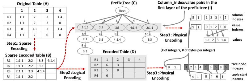
Figure 3: A running example of the TOC encoding process. TOC has three components: sparse encoding, logical encoding, and physical encoding. The red dotted lines connect these components. Sparse encoding encodes the original table A to the sparse encoded table B. Logical encoding encodes B to the encoded table D. It also outputs I, which is the column_index:value pairs in the first layer of the prefix tree C. Physical encoding encodes I and D to physical bytes efficiently.

In this section, we introduce our tuple-oriented compression (TOC). The goal of TOC is to (1) compress a mini-batch as much as possible and (2) preserve the row/column boundaries in the underlying tabular data so that matrix operations can directly operate on the compressed representation without decompression overheads. Following the popular sparse row technique [37], we use sparse encoding as a starting point, and introduce two new techniques: logical encoding and physical encoding. Figure 3 demonstrates a running example of the encoding process.

For sparse encoding, we ignore the zero values and then prefix each non-zero value with its column index. We call the value with its column index prefix as column_index:value pair. For example, in Figure 3, tuple R2 - [1.1, 2, 3, 0] is encoded as [1:1.1, 2:2, 3:3], where 1:1.1 is a column_index:value pair. As a result of sparse encoding, the original table (A) in Figure 3 is converted to the sparse encoded table (B).

3.1 Logical Encoding

The sparse encoded table (e.g., B in Figure 3) can be further compressed logically. The key idea is that there are repeating sequences of column_index:value pairs across tuples in the table. For example, R2 and R4 in the table B both have the same sequence [1:1.1, 2:2]. Thus, these occurrences of the same sequence can be encoded as the same index pointing to a dictionary entry, which represents the original sequence. Since many of these sequences have common prefixes, a prefix tree is used to store all the sequences. Finally, each original tuple is encoded as a vector of indexes pointing to prefix tree nodes.

We present the prefix tree structure and its APIs in § 3.1.1. In § 3.1.2, we present the actual prefix tree encoding algorithm, including how to dynamically build the tree and encode tuples. The comparison between our prefix tree encoding algorithm and LZW is presented in § 3.1.3.

3.1.1 Prefix Tree Structure and APIs

Each node of the prefix tree has an index. Except for the root node, each node stores a column_index:value pair as its key. Each node also represents a sequence of column_index:value pairs, which are obtained by concatenating the keys from the prefix tree root to the node itself. For example, in the prefix tree C in Figure 3, the left bottom tree node has index 9, stores key 3:3, and represents the sequence of column_index:value pairs [1:1.1, 2:2, 3:3].

The prefix tree supports two main APIs: AddNode and GetIndex.

• $n^{\prime}=\textbf{AddNode}(n,k)$. This API creates a new prefix tree node which has key $k$ and is a child of the tree node with index $n$. It also returns the index of the newly created tree node in $n^{\prime}$, which is assigned from a sequence number starting from 0.

• $n^{\prime}=\textbf{GetIndex}(n,k)$. This API looks up the tree node which has key $k$ and is a child of the tree node with index $n$. It also returns the index of the found tree node in $n^{\prime}$. If there is no such node, it returns -1.

The implementation of AddNode is straightforward. The implementation of GetIndex is more involved, and we use a standard technique reported in [7]. In essence, for each tree node, we create a hash map mapping from its child node keys to its child node indexes.

3.1.2 Prefix Tree Encoding Algorithm

Our prefix tree encoding algorithm encodes the sparse encoded table (e.g., B in Figure 3) to an encoded table (e.g., D in Figure 3). During the encoding process, we build a prefix tree (e.g., C in Figure 3) and each original tuple is encoded as a vector of indexes pointing to prefix tree nodes. Algorithm 1 presents the pseudo-code of the algorithm. Figure 3 presents a running example of executing the algorithm and encoding table B to table D.

The prefix tree encoding algorithm has two main phases. In phase i@ (line 5 to line 8 of Algorithm 1), we initialize the prefix tree with all the unique  column_index:value pairs in the sparse encoded table as the children of the root node.

In phase ii@ (line 9 to line 17 of Algorithm 1), we leverage the repeated sequences of the tuples so that the same sequence, for example R2 and R4 in Figure 3 both have the sequence [1:1, 2:2], is encoded as the same index to the prefix tree node. At its heart, we scan all the tuples to detect if part of the tuple can match a sequence that already exists in the prefix tree and build up the prefix tree along the way. We use the function LongestMatchFromTree in Algorithm 1, to find the longest sequence in the prefix tree that matches the sequence in the tuple t starting from the position $i$. The function returns the tree node index of the longest match in $n$, and the next matching starting position in $j$. If $j\neq len(\textbf{t})$, we add a new node to the prefix tree which is the child of the tree node with index $n$ and has key $\textbf{t}[j]$ to capture this new sequence in the tuple t. In this way, later tuples can leverage this new sequence. Note that the longest match found is at least of length one because we store all the unique column_index:value pairs as the children of the root node in phase i@. Table 2 gives a running example of executing Algorithm 1 on table B in Figure 3.

Our prefix tree encoding and LZW are both linear algorithms in the sense that each input unit is read at most twice and the operation on each input unit is constant. So the time complexity of Algorithm 1 is $\mathcal{O}(|\textbf{B}|)$, where $|\textbf{B}|$ is the number of column_index:value pairs in the sparse encoded table B.

Algorithm 1 Prefix Tree Encoding Algorithm

1:function PrefixTreeEncode(B)

2:     inputs: sparse encoded table B

3:     outputs: column_index:value pairs in the first layer

4:              of the prefix tree I and encoded table D

5:     Initialize C with a root node with index 0.

6:     for each tuple t in B do $\triangleright$ phase i@: initialization

7:         for each column_index:value pair t[$i$] in t do

8:              if C.GetIndex($0,\textbf{t}[i]$) = -1 then

9:                  C.AddNode($0,\textbf{t}[i]$)                             

10:     for each tuple t in B do $\triangleright$ phase ii@: encoding

11:         $i\leftarrow 0$ $\triangleright$ set the matching starting position

12:         $\textbf{D[t]}\leftarrow[]$ $\triangleright$ initialize as an empty vector

13:         while $i<$ len(t) do

14:              $(n,j)\leftarrow$ LongestMatchFromTree(t, $i$, C)

15:              D[t].append($n$)

16:              if $j<$ len(t) then

17:                  C.AddNode($n$, t[$j$])               

18:              $i\leftarrow j$               

19:     I $\leftarrow$ first_layer(C)

20:     return(I, D)

21:

22:function LongestMatchFromTree(t, $i$, C)

23:     inputs: input tuple t, matching starting position $i$

24:              in t, and prefix tree C

25:     outputs: index of the tree node of the longest match

26:              $n$ and next matching starting position $j$

27:     $j\leftarrow i$

28:     $n^{\prime}\leftarrow$ C.GetIndex($0$, t[$j$]) $\triangleright$ matching 1st element

29:     do

30:         $n\leftarrow n^{\prime}$

31:         $j\leftarrow j+1$ $\triangleright$ try matching the next element

32:         if $j<$ len(t) then

33:              $n^{\prime}\leftarrow$ C.GetIndex($n$, t[$j$]) $\triangleright$ return -1 if such a tree node does not exist

34:         else

35:              $n^{\prime}\leftarrow-1$ $\triangleright$ reaching the end of tuple t          

36:     while $n^{\prime}\neq-1$

37:     return($n$, $j$)

Table 2: We show the steps of running Algorithm 1 on table B in Figure 3. We omit the phase i@ of the algorithm, which initializes the prefix tree with nodes: 1 $\rightarrow$ [1:1.1], 2 $\rightarrow$ [2:2], 3 $\rightarrow$ [3:3], 4 $\rightarrow$ [4:1.4], and 5 $\rightarrow$ [2:1.1], where the left side of the arrow is the tree node index and the right side of the arrow is the sequence of column_index:value pairs represented by the tree node. Each entry here illustrates an iteration of the while loop (line 12 - line 17) of Algorithm 1. Column $i$ is the starting position of the tuple that we try to match the sequence in the prefix tree. Column LMFromTree shows the index and the corresponding sequence of the found longest match by the function LongestMatchFromTree. Column App is the appended tree node index for encoding the tuples in table B. Column AddNode shows the index and the corresponding sequence of the newly added tree node.

	$i$	LMFromTree	App	AddNode
R1	0	1 $\rightarrow$ [1:1.1]	1	6 $\rightarrow$ [1:1.1, 2:2]
	1	2 $\rightarrow$ [2:2]	2	7 $\rightarrow$ [2:2, 3:3]
	2	3 $\rightarrow$ [3:3]	3	8 $\rightarrow$ [3:3, 4:1.4]
	3	4 $\rightarrow$ [4:1.4]	4	NOT called
R2	0	6 $\rightarrow$ [1:1.1, 2:2]	6	9 $\rightarrow$ [1:1.1, 2:2, 3:3]
	2	3 $\rightarrow$ [3:3]	3	NOT called
R3	0	5 $\rightarrow$ [2:1.1]	5	10 $\rightarrow$ [2:1.1, 3:3]
	1	8 $\rightarrow$ [3:3, 4:1.4]	8	NOT called
R4	0	6 $\rightarrow$ [1:1.1, 2:2]	6	NOT called

3.1.3 Comparisons with Lempel-Ziv-Welch (LZW)

Our prefix tree encoding algorithm is inspired by the classical compression scheme LZW. However, a key difference between LZW and our algorithm is that we preserve the row and column boundaries in the underlying tabular data, which is crucial to directly operate matrix operations on the compressed representation. For examples, our algorithm encodes each tuple separately (although the dictionary is shared) to respect the row boundaries, and the compression unit is a column_index:value pair to respect the column boundaries. In contrast, LZW simply encodes a blob of bytes without preserving any structure information. The reason for that is LZW was invented primarily for string/text compression. There are other several noticeable differences between our algorithm and LZW, which are summarized in Table 3.

Table 3: Differences between LZW and our prefix tree encoding. c-v stands for column-index:value.

	LZW	Ours
Input	bytes	sparse encoded table
Encode unit	8 bits	c-v pair
Tree init.	all values of 8 bits	all unique c-v pairs
Tuple bound.	lost	preserved
Output	a vector of codes	encoded table & prefix tree first layer

3.2 Physical Encoding

The output of the logical encoding (i.e., I and D in Figure 3) can be further encoded physically to reduce sizes. We use two simple techniques—bit packing [26] and value indexing [21]— that can reduce sizes without incurring significant overheads when accessing the original values.

We notice that some information in I and D can be stored using arrays of non-negative integers, and these integers are typically small. For example, the maximal column index in I of Figure 3 is 4, so 1 byte is enough to encode a single integer. Bit packing is used to encode these arrays of small non-negative integers efficiently. Specifically, we use $\lceil\frac{1}{8}*\log_{2}^{\text{maximal\_integer+1}}\rceil$ bytes to encode each non-negative integer in an array. Each encoded array has a header that tells the number of integers in the array and the number of bytes used per integer. More advanced encoding methods such as Varint [12] and SIMD-BP128 [26], can also be used, and point to interesting directions for future work.

Value indexing is essentially a dictionary encoding technique. That is, we store all the unique values (excluding column indexes) in the column_index:value pairs (e.g., I in Figure 3) in an array. Then, we replace the original values with the indexes pointing to the values in the array.

Figure 3 illustrates an example of how we encode the input (e.g., I and D) to physical bytes. For I, the column indexes are encoded using bit packing, while the values are encoded using value indexing. The value indexes from applying value indexing are also encoded using bit packing. For D, we concatenate the tree node indexes from all the tuples and encode them all together using bit packing. We also encode the tuple starting indexes using bit packing.

4 Matrix Operation Execution

In this section, we introduce how to execute matrix operations on the TOC output. Most of the operations can directly operate on the compressed representation without decoding the original matrix. This direct execution avoids the tedious and expensive decoding process and reduces the runtime to execute matrix operations and MGD.

Let $A$ be a TOC compressed matrix, $c$ be a scalar, $v/M$ be an uncompressed vector/matrix respectively, we discuss four common classes of matrix operations:

1. Sparse-safe element-wise [14] operations (e.g., $A.*c$ and $A.^{2}$).

2. Right multiplication operations (e.g., $A\cdot v$ and $A\cdot M$).

3. Left multiplication operations (e.g., $v\cdot A$ and $M\cdot A$).

4. Sparse-unsafe element-wise operations [14] (e.g., $A.+c$ and $A+M$).

Informally speaking, sparse-safe operation means that zero elements in the matrix remain as zero after the operation; sparse-unsafe operation means that zero elements in the matrix may not be zero after the operation.

Figure 4 gives an overview of how to execute different matrix operations on the TOC output. The first three classes of operations can directly operate over the compressed representation without decoding the original matrix. The last class of operations needs to decode the original matrix. However, it is less likely to be used for training machine learning models because it changes the input data.

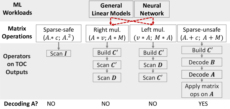
Figure 4: An overview of how to execute different matrix operations on the TOC output. For sparse-safe element-wise operations, right multiplication operations, and left multiplication operations, we can execute them on the TOC output directly. For sparse-unsafe element-wise operations, we need to fully decode the input $A$ and then apply the operation on $A$.

4.1 Shared Operators

In this subsection, we discuss some shared operators for executing matrix operations on the TOC output.

4.1.1 Access Values of I and D From Physical Bytes

As shown in Figure 4, executing many matrix operations requires scanning I or D, which are encoded to physical bytes using bit packing and value indexing as explained in § 3.2. Thus, we briefly discuss how to access values of I and D from encoded physical bytes.

To access a non-negative integer encoded using bit packing, one can simply seek to the starting position of the integer, and cast its bytes to uint_8, uint_16, or uint_32 respectively. Unfortunately, most programming languages do not support uint_24 natively. Nevertheless, one can copy the bytes into an uint_32 and mask its leading byte as zero.

To access values encoded using value indexing, one can look up the array which stores the unique values using the value indexes.

4.1.2 Build Prefix Tree For Decoding

As shown in Figure 4, executing all matrix operations except for sparse-safe element-wise operations needs to build the prefix tree $\mathbf{C^{\prime}}$, which is a simplified variant of the prefix tree C built during encoding. Each node in $\mathbf{C^{\prime}}$ has the same index and key with the node in C. The difference is that each node in $\mathbf{C^{\prime}}$ stores the index to its parent, but it does NOT store indexes to its children. Table 4 demonstrates an example of $\mathbf{C^{\prime}}$.

Table 4: An example of $\mathbf{C^{\prime}}$, which is a simplified variant of C in Figure 3. Each node in $\mathbf{C^{\prime}}$ only stores the index to its parent but NOT indexes to its children.

Index	0	1	2	3	4	5	6	7	8	9	10
Key		1:1.1	2:2	3:3	4:1.4	2:1.1	2:2	3:3	4:1.4	3:3	3:3
ParentIndex		0	0	0	0	0	1	2	3	6	5

Algorithm 2 presents how to build $\mathbf{C^{\prime}}$. There are two main phases in Algorithm 2. In phase i@, $\mathbf{C^{\prime}}$ and F are both initialized by I, where F stores the first column_index:value pair of the sequence represented by each tree node.

In phase ii@, we scan D to build $\mathbf{C^{\prime}}$ mimicking how C is built in Algorithm 1. From line 11 to line 13 of Algorithm 2, we add a new prefix tree node indexed by idx_seq_num. More specifically, the new tree node is a child of the tree node indexed by D[$i$][$j$] (line 11), the first column_index:value pair of the sequence represented by the new tree node is the same with its parent (line 12), and the key of the new tree node is the first column_index:value pair of the sequence represented by the next tree node indexed by D[$i$][$j+1$] (line 13).

Algorithm 2 Build Prefix Tree $\mathbf{C^{\prime}}$

1:function BuildPrefixTree(I, D)

2:     inputs: column_index:value pairs in the first layer

3:              of the prefix tree I and encoded table D

4:     outputs: A prefix tree used for decoding $\mathbf{C^{\prime}}$

5:     for $i\leftarrow$ 1 to len(I) do $\triangleright$ phase i@: initialize with I

6:         $\mathbf{C^{\prime}}[i]$.key $\leftarrow\textbf{I}[i-1]$

7:         $\mathbf{C^{\prime}}[i]$.parent $\leftarrow 0$

8:         $\textbf{F}{[i]}\leftarrow\textbf{I}[i-1]$ $\triangleright$ F stores the first column_index:value pair of the sequence of the node      

9:     idx_seq_num $\leftarrow$ len(I) + 1

10:     for $i\leftarrow$ 0 to len(D) - 1 do $\triangleright$ phase ii@: build $\mathbf{C^{\prime}}$

11:         for $j\leftarrow$ 0 to len(D[$i$]) -2  do $\triangleright$ skip last element

12:              $\mathbf{C^{\prime}}$[idx_seq_num].parent $\leftarrow$ D[$i$][$j$]

13:              F[idx_seq_num] $\leftarrow$ F[D[$i$][$j$]]

14:              $\mathbf{C^{\prime}}$[idx_seq_num].key $\leftarrow$ F[D[$i$][$j+1$]]

15:              idx_seq_num $\leftarrow$ idx_seq_num + 1               

16:     return ($\mathbf{C^{\prime}}$)

4.2 Sparse-safe Element-wise Operations

To execute sparse-safe element-wise operations (e.g., $A.*c$ and $A.^{2}$) on the TOC output directly, one can simply scan and modify I because all the unique column_index:value pairs in $A$ are stored in I. Algorithm  3 demonstrates how to execute matrix times scalar operation (i.e., $A.*c$) on the TOC output. Algorithms for other sparse-safe element-wise operations are similar.

Algorithm 3 Execute matrix times scalar operation (i.e., $A.*c$) on the TOC output.

1:function MatrixTimesScalar(I, c)

2:     inputs: column_index:value pairs in the first layer

3:              of the prefix tree I and a scalar c

4:     outputs: the modified I

5:     for $i\leftarrow$ 0 to len(I) -1 do

6:         $\textbf{I}[i]$.value $\leftarrow$ $\textbf{I}[i]$.value * c      

7:     return(I)

4.3 Right Multiplication Operations

We first do some mathematical analysis to transform the uncompressed execution of right multiplication operations to the compressed execution that operates directly on the TOC output without decoding the original table. The analysis also proves the algorithm correctness since the algorithm follows the transformed form directly. Then, we demonstrate the detailed algorithm. In the rest of this subsection, we use $A\cdot v$ as an example. We put the result of $A\cdot M$ (similar to $A\cdot v$) in Appendix B for brevity.

Theorem 1.

Let $A\in\Re^{n\times m}$, $v\in\Re^{m\times 1}$, D be the output of TOC on $A$, $\mathbf{C^{\prime}}$ be the prefix tree built for decoding, $\mathbf{C^{\prime}}[i].seq$ be the sequence of the tree node defined in § 3.1.1, $\mathbf{C^{\prime}}[i].key$ be the key of the tree node defined in § 4.1.2, and $\mathbf{C^{\prime}}[i].parent$ be the parent index of the tree node defined in § 4.1.2. Note that $\mathbf{C^{\prime}}[i].key$ and $\mathbf{C^{\prime}}[i].seq$ are both sparse representations of vectors (i.e., $\mathbf{C^{\prime}}[i].key\in\Re^{1\times m}$ and $\mathbf{C^{\prime}}[i].seq\in\Re^{1\times m}$). Define function $\mathcal{F}(x):\aleph\rightarrow\Re$ to be

$$\mathcal{F}(x)=\mathbf{C^{\prime}}[x].seq\cdot v,x=1,2,...,\mathrm{len}(\mathbf{C^{\prime}})-1.$$ (4)

Then, we have

$$A[i,:]\cdot v= \sum_{j=0}^{\mathrm{len}(\mathbf{D}[i,:])-1}\mathcal{F}(\mathbf{D}[i][j]),i=0,1,...,n-1$$ (5)

and

$$\mathbf{C^{\prime}}[i].seq= ~{}\mathbf{C^{\prime}}[i].key+\mathbf{C^{\prime}}[\mathbf{C^{\prime}}[i].parent].seq,$$

$$i=1,2,...,\mathrm{len}(\mathbf{C^{\prime}})-1.$$ (6)

Proof.

See Appendix A.1 ∎

Remark on Theorem 1. $A\cdot v$ can be directly executed on the TOC output following Equation 5 by scanning $\mathbf{C^{\prime}}$ first and scanning $\mathbf{D}$ second. The detailed steps are demonstrated in Algorithm 4.

First, we scan $\mathbf{C^{\prime}}$ to compute $\mathcal{F}$ function defined in Equation 4 (lines 5-7 in Algorithm 4). The dynamic programming technique is used following Equation 6. Specifically, we use H[$i$] to remember the computed value of $\mathcal{F}(i)$. We compute each H[$i$] as the sum of $\mathbf{C^{\prime}}[i].key\cdot v$ and H[$\mathbf{C^{\prime}}$[$i$].parent], which is computed already.

Second, we scan D to compute $A\cdot v$ and store it in R following Equation 5 (lines 8-11 in Algorithm 4). For each D[$i$][$j$], we simply add H[D[$i$][$j$]] to R[$i$].

Algorithm 4 Execute matrix times vector operation (i.e., $A\cdot v$) on the TOC output.

1:function MatrixTimesVector(D, I, $v$)

2:     inputs: column_index:value pairs in the first layer of the prefix tree I, encoded table D, and vector $v$

3:     outputs: the result of $A\cdot v$ in R

4:     $\mathbf{C^{\prime}}\leftarrow$ BuildPrefixTree(I, D)

5:     H $\leftarrow\overrightarrow{0}$ $\triangleright$ initialize as a zero vector

6:     for $i$ = 1 to len($\mathbf{C^{\prime}}$)-1 do $\triangleright$ scan $\mathbf{C^{\prime}}$ to compute H

7:         H[$i$] $\leftarrow\mathbf{C^{\prime}}$[$i$].key $\cdot v$ + H[$\mathbf{C^{\prime}}$[$i$].parent]      

8:     R $\leftarrow\overrightarrow{0}$ $\triangleright$ initialize as a zero vector

9:     for $i$ = 0 to len(D)-1 do $\triangleright$ scan D to compute R

10:         for $j$ = 0 to len(D[$i$,:])-1 do

11:              R[$i$] $\leftarrow$ R[$i$] + H[D[$i$][$j$]]               

12:     return(R)

4.4 Left Multiplication Operations

We first give the mathematical analysis and then present the detailed algorithm. The reason for doing so is similar to that is given in § 4.3. We only demonstrate the result of $v\cdot A$ and put the result of $M\cdot A$ to Appendix B for brevity.

Theorem 2.

Let $A\in\Re^{n\times m}$, $v\in\Re^{1\times n}$, D be the output of TOC on $A$, $\mathbf{C^{\prime}}$ be the prefix tree built for decoding, $\mathbf{C^{\prime}}[i]$.seq be the sequence of the tree node defined in § 3.1.1, $\mathbf{C^{\prime}}[i].key$ be the key of the tree node defined in § 4.1.2, and $\mathbf{C^{\prime}}[i].parent$ be the parent index of the tree node defined in § 4.1.2. Note that $\mathbf{C^{\prime}}[i].key$ and $\mathbf{C^{\prime}}[i].seq$ are both sparse representations of vectors (i.e., $\mathbf{C^{\prime}}[i].key\in\Re^{1\times m}$ and $\mathbf{C^{\prime}}[i].seq\in\Re^{1\times m}$). Define function $\mathcal{G}(x):\aleph\rightarrow\Re$ to be

$$\mathcal{G}(x)=\sum_{\begin{subarray}{c}\mathbf{D}[i,j]=x,\forall i\in\aleph,\forall j\in\aleph\end{subarray}}v[i],~{}x=1,2,...,\mathrm{len}(\mathbf{C^{\prime}})-1.$$ (7)

Then, we have

$$v\cdot A= \sum_{i=1}^{\mathrm{len}(\mathbf{C^{\prime}})-1}\mathbf{C^{\prime}}[i].seq\cdot\mathcal{G}(i).$$ (8)

Proof.

See Appendix A.2. ∎

Remark on Theorem 2. We can compute $v\cdot A$ following Equation 8 by simply scanning D first and scanning $\mathbf{C^{\prime}}$ second. Algorithm 5 presents the detailed steps. First, we scan D to compute function $\mathcal{G}$ defined in Equation 7. Specifically, we initialize $\mathbf{H}$ as a zero vector, and then add $v[i]$ to $\mathbf{H}[\mathbf{D}[i][j]]$ for each $\mathbf{D}[i][j]$ (lines 6-8 in Algorithm 5). After this step is done, $\mathcal{G}(i)=\mathbf{H}[i],i$ = 1, 2, $\dots$, len$(\mathbf{C^{\prime}})-1$.

Second, we scan $\mathbf{C^{\prime}}$ backwards to actually compute $v\cdot A$ and store it in R following Equation 8 (lines 10-12 in Algorithm 5). The dynamic programming technique is used following Equation 6. Specifically, for each $\mathbf{C^{\prime}}[i]$, we add $\mathbf{C^{\prime}}[i].key\cdot\mathbf{H}[i]$ to R and add $\mathbf{H}[i]$ to $\mathbf{H}[\mathbf{C^{\prime}}[i].parent]$.

Algorithm 5 Execute vector times matrix operation (i.e., $v\cdot A$) on the TOC output.

1:function VectorTimesMatrix(D, I, $v$)

2:     inputs: column_index:value pairs in the first layer of the prefix tree I, encoded table D, and vector $v$

3:     outputs: the result of $v\cdot A$ in R

4:     $\mathbf{C^{\prime}}\leftarrow$ BuildPrefixTree(I, D)

5:     H $\leftarrow\overrightarrow{0}$ $\triangleright$ initialize as a zero vector

6:     for $i$ = 0 to len(D)-1 do $\triangleright$ scan D to compute H

7:         for $j$ = 0 to len(D[$i$,:]) -1 do

8:              H[D[$i$][$j$]] $\leftarrow$ $v$[$i$] + H[D[$i$][$j$]]               

9:     R $\leftarrow\overrightarrow{0}$ $\triangleright$ initialize as a zero vector

10:     for $i$ = len($\mathbf{C^{\prime}}$) -1 to 1 do $\triangleright$ scan $\mathbf{C^{\prime}}$ to compute R

11:         R $\leftarrow$ R + $\mathbf{C^{\prime}}$[$i$].key $\cdot$ H[$i$]

12:         H[$\mathbf{C^{\prime}}[i]$.parent] $\leftarrow$ H[$\mathbf{C^{\prime}}$[i].parent] + H[$i$]      

13:     return(R)

4.5 Sparse-unsafe Element-wise Operations

For sparse-unsafe element-wise operations (e.g., $A.+c$ and $A+M$), we need to fully decode $A$ first and then execute the operations on $A$. Although this process is slow due to the tedious decoding step, fortunately, sparse-unsafe element-wise operations are less likely to be used for training ML models because the input data is changed. Algorithm 6 presents the detailed steps.

Algorithm 6 Execute matrix plus scalar element-wise operation (i.e., $A.+c$) on the TOC output.

1:function MatrixPlusScalar(D, I, $c$)

2:     inputs: column_index:value pairs in the first layer of the prefix tree I, encoded table D, and scalar $c$

3:     outputs: the result of $A.+c$ in R

4:     $\mathbf{C^{\prime}}\leftarrow$ BuildPrefixTree(I, D)

5:     for $i$ = 0 to len(D)-1 do

6:         B[$i$] $\leftarrow$ [] $\triangleright$ initialize B[$i$] as an empty vector

7:         for $j$ = 0 to len(D[$i$,:])-1 do

8:              reverse_seq $\leftarrow$ []

9:              tree_index $\leftarrow$ D[$i$][$j$]

10:              while tree_index $\neq$ 0 do $\triangleright$ backtrack $\mathbf{C^{\prime}}$ to get the reversed sequence of the tree node D[$i$][$j$]

11:                  reverse_seq.Append($\mathbf{C^{\prime}}$[tree_index].key)

12:                  tree_index $\leftarrow\mathbf{C^{\prime}}$[tree_index].parent               

13:              for $k$ = len(reverse_seq)-1 to 0 do

14:                  B[$i$].Append(reverse_seq[$k$])                             

15:     $A\leftarrow$ TransformToDense(B)

16:     R $\leftarrow A.+c$

17:     return(R)

4.6 Time Complexity Analysis

We give detailed time complexity analysis of different matrix operations except for $A\cdot M$ and $M\cdot A$, which we put to Appendix C for brevity. For $A.*c$, we only need to scan I, so the time complexity is $\mathcal{O}(|\mathbf{I}|)$.

For $A\cdot v$ and $v\cdot A$, we need to build $\mathbf{C^{\prime}}$ , scan $\mathbf{C^{\prime}}$, and scan D. As shown in Algorithm 2, building $\mathbf{C^{\prime}}$ needs to scan I and D, and $|\mathbf{C^{\prime}}|=|\mathbf{I}|+|\mathbf{D}|$. So the complexity of building and scanning $\mathbf{C^{\prime}}$ are $\mathcal{O}(|\mathbf{I}|+|\mathbf{D}|)$. Overall, the complexity of $A\cdot v$ and $v\cdot A$ are $\mathcal{O}(|\mathbf{I}|+|\mathbf{D}|)$. This indicates that the computational redundancy incurred by the data redundancy is generally avoided by TOC matrix execution algorithms. Thus, theoretically speaking, TOC matrix execution algorithms have good performance when there are many data redundancies.

For $A.+c$, we need to decompress A first. Similar to LZW, the decompression of TOC is linear in the sense that each element has to be outputted and the cost of each output element is constant. Thus, the complexity of decompressing A is $\mathcal{O}(|\mathbf{A}|)$. Overall, the complexity of $A.+c$ is also $\mathcal{O}(|\mathbf{A}|)$.

5 Experiments

In this section, we answer the following questions:

1. Can TOC compress mini-batches effectively?

2. Can common matrix operations be executed efficiently on TOC compressed mini-batches?

3. Can TOC reduce the end-to-end MGD runtimes significantly for training common machine learning models?

4. Can TOC compress/decompress mini-batches fastly?

Summary of Answers. We answer these questions positively by conducting extensive experiments. First, on datasets with moderate sparsity, TOC reduces mini-batch sizes notably with compression ratios up to 51x. Compression ratios of TOC are up to 3.8x larger than the state-of-the-art light-weight matrix compression schemes, and comparable to general compression schemes such as Gzip. Second, the matrix operation runtime of TOC is comparable to the light-weight matrix compression schemes, and up to 20,000x better than the state-of-the-art general compression schemes. Third, TOC reduces the end-to-end MGD runtimes by up to 1.4x, 5.6x, and 4.8x compared to the state-of-the-art compression schemes for training Neural network, Logistic regression, and Support vector machine, respectively. TOC also reduces the MGD runtimes by up to 10.2x compared to the best encoding methods used in popular machine learning systems: Bismarck, ScikitLearn, and TensorFlow. Finally, the compression speed of TOC is much faster than Gzip but slower than Snappy, whereas the decompression speed of TOC is faster than both Gzip and Snappy.

Datasets. We use six real-world datasets. The first four datasets we chose have moderate sparsity, which is a typical phenomenon for enterprise machine learning [4, 17]. Rcv1 and Deep1Billion represent the extremely sparse and dense dataset respectively. Table 5 lists the dataset statistics.

Table 5: Dataset statistics. Except for Deep1Billion, which is in the binary format, we report the sizes of the datasets stored in the text format. Sparsity is defined as $\frac{\#\text{ of non zero values}}{\#\text{ of total values}}$.

Dataset	Dimensions	Size	Sparsity
US Census [14]	2.5 M * 68	0.46 GB	0.43
ImageNet [14]	1.2 M * 900	2.8 GB	0.31
Mnist8m [14]	8.1 M * 784	11.3 GB	0.25
Kdd99 [28]	4 M * 42	1.6 GB	0.39
Rcv1 [3]	800 K * 47236	0.96 GB	0.0016
Deep1Billion [5]	1 B * 96	475 GB	1.0

Compared Methods. We compare TOC with one baseline (DEN), four light-weight matrix compression schemes (CSR, CVI, DVI, and CLA), and two general compression schemes (Snappy and Gzip). A brief summary of these methods is as follows:

1. DEN: This is the standard dense binary format for dense matrices. We store the matrix row by row and each value is encoded using IEEE-754 double format. Categorical features are encoded using the standard one-hot (dummy) encoding [16].

2. CSR: This is the standard compressed sparse row encoding for sparse matrices. We store the matrix row by row. For each row, we only store the non-zero values and associated column indexes.

3. CVI: This format is also called as CSR-VI [21, 14]. We first encode the matrix using CSR and then encode non-zero values via the value indexing in Section 3.2.

4. DVI: We first encode the matrix using DEN and then encode the values via the value indexing in Section 3.2.

5. CLA: This method [14] divides the matrix into different column-groups and compresses each column-group column-wisely. Note that matrix operations can be executed on compressed CLA matrices directly.

6. Snappy: We compress the serialized bytes of DEN using Snappy.

7. Gzip: We use Gzip to compress the serialized bytes of DEN.

Machine and System Setup. All experiments were run on Google cloud using a typical machine with a $4$ core, $2.2$ GHz Intel Xeon CPU, $15$GB RAM (unless otherwise specified), and OS Ubuntu $14.04.1$. We did not choose a more powerful machine because of the higher cost. For example, our machine costs $$131$ per month, while a machine with $4$ cores and $180$ GB RAM costs $$912$ per month. Thus, our techniques can save costs for ML workloads, especially in such cloud settings.

Our techniques were implemented in C++ and compiled using g++ $4.8.4$ with the flag O3 optimization. We also compare with four machine learning systems: ScikitLearn 0.19.1, Systemml 1.3.0, Bismarck 2.0, and TensorFlow. Furthermore, we integrate TOC into Bismarck to realize fair comparison. We put the integration detail into Appendix D.1 for brevity.

5.1 Compression Ratios

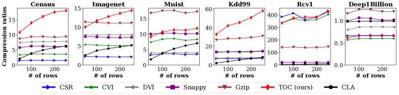
Figure 5: Compression ratios of different methods on mini-batches with varying sizes.

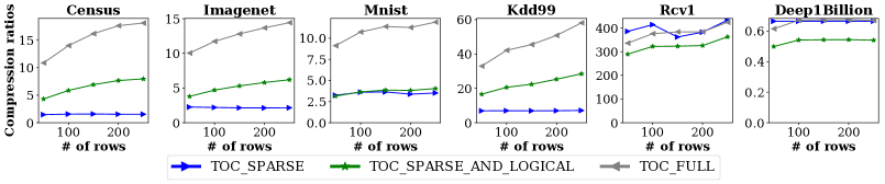
Figure 6: Compression ratios of TOC variants on varying size mini-batches. TOC_SPARSE uses sparse encoding. TOC_SPARSE_AND_LOGICAL uses sparse and logical encoding. TOC_FULL uses all the encoding techniques.

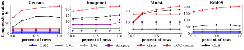
Figure 7: Compression ratios of different methods on large mini-batches. The x-axis is the percent of rows of the whole dataset in the mini-batch.

Setup. We are not aware of a first-principle way in literature to set mini-batch sizes (# of rows in a mini-batch). In practice, the mini-batch size typically depends on system constraints (e.g. number of CPUs) and is set to some number ranging from 10 to 250 [30]. Thus, we tested five mini-batch sizes 50, 100, 150, 200, and 250, which cover the most common use cases. Compression ratio is defined as the uncompressed mini-batch size (encoded using DEN) over the compressed mini-batch size. We implemented DEN, CSR, CVI, and DVI by ourselves but use CLA from Systemml and Gzip/Snappy from standard libraries. We tested mini-batches from all the real datasets with the sizes mentioned above.

Overall Results. Figure 5 presents the overall results. For the very sparse dataset Rcv1, CSR is the best encoding method and TOC’s performance is similar to CSR. For the very dense dataset Deep1Billion, which does not contain repeated subsequences of column values, Gzip is the best method but it only achieved a marginal 1.15x compression ratio. CSR and TOC have similar performance because of the sparse encoding.

For the other 4 datasets with moderate sparsity, TOC has larger compression ratios than all the other methods except on Mnist, where TOC is inferior to Gzip. The main reason is that Mnist does not contain many repeated subsequences of column values that TOC logical encoding can exploit, this is also verified by the ablation study in Figure 6.

Overall, TOC is suitable for datasets of moderate sparsity, which are commonly used datasets in enterprise ML. TOC is not suitable for very sparse datasets and very dense datasets that do not contain repeated subsequences of columns values. Note that these datasets are challenging for other compression methods too. Nevertheless, one can simply test TOC on a mini-batch sample and figure out if TOC is suitable for the dataset.

Ablation Study. We conduct an ablation study to show the effectiveness of different components (e.g., sparse encoding, logical encoding, and physical encoding) in TOC. TOC_SPARSE_AND_LOGICAL compresses better than TOC_SPARSE. TOC_FULL with all the encoding techniques compresses the best. This shows the effectiveness of all our encoding components. Figure 6 shows the ablation study results.

Large Mini-batches. We compare different compression methods on large mini-batches. Figure 7 shows the results. As the mini-batch size grows, TOC becomes more competitive. When the percent of rows of the whole dataset in the mini-batch is 1.0, this is essentially batch gradient descent (BGD) and TOC has the best compression ratio in this case. This shows the potential of applying TOC to BGD related workloads.

5.2 Matrix Operation Runtimes

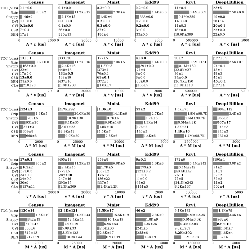
Figure 8: Average runtimes (5 runs) and 95% confidence intervals to execute different matrix operations on compressed mini-batches. From top to bottom are different matrix operations, where $c$ is a scalar, $v$ is an uncompressed vector, $M$ is an uncompressed matrix, and $A$ is the compressed matrix. From left to right are different datasets.

Setup. We tested three classes of matrix operations: sparse-safe element-wise operation ($A\cdot c$), left multiplication operations ($v\cdot A$ and $M\cdot A$), and right multiplication operations ($A\cdot v$ and $A\cdot M$), where $c$ is a scalar, $v$ is an uncompressed vector, $M$ is an uncompressed matrix, and $A$ is the compressed mini-batch. We set mini-batch size as 250 (results for other mini-batch sizes are similar). Figure 8 presents the results.

Sparse-safe Element-wise Operations ($A\cdot c$). In general, DVI, CVI, and TOC are fastest methods. This shows the effectiveness of value indexing [21] which is used by all these methods. It is noteworthy that TOC can be four orders of magnitude faster than Gzip and Snappy (e.g. on Imagenet). The slowness of these general compression schemes is caused by their significant decompression overheads.

Right Multiplication Operations ($A\cdot v$ and $A\cdot M$). For $A\cdot v$, CSR/DEN are the best methods for Rcv1/Deep1Billion due to their extreme sparsity/density respectively. For the remaining datasets of moderate sparsity, DEN, CSR, CVI, DVI, and TOC are fastest methods. CLA and general compression schemes like Snappy and Gzip are much slower. We do see that TOC is 2-3x slower than CSR on dataset Imagenet and Mnist. There are two main reasons for the slowness. First, building the prefix tree $\mathbf{C^{\prime}}$ in TOC takes extra time. Second, TOC compression ratios over CSR compression ratios are relatively small on these datasets, which render the computational redundancies exploited by TOC on these datasets also smaller.

For $A\cdot M$, we set the row size of $M$ as 20. TOC is consistently the fastest on all the datasets except for Rcv1 and Deep1Billion due to its extreme sparsity/density. CLA in Systemml does not support $A\cdot M$ yet, thus CLA is excluded.

Left Multiplication Operations ($v\cdot A$ and $M\cdot A$). The results of left multiplication operations are similar to right multiplication operations. Thus, we leave them for brevity.

Summary. Overall, TOC achieves the best runtime performance on operations: $A\cdot c$, $A\cdot M$, and $M\cdot A$. TOC can be 2-3x slower than the fastest method on operations $A\cdot v$ and $v\cdot A$. However, as we will show shortly in § 5.3, it has negligible effect in the context of overall ML training time.

5.3 End-to-End MGD Runtimes

In this subsection, we discuss the end-to-end MGD runtime performance with different compression schemes.

Compared Methods. We compare TOC with DEN, CSR, CVI, DVI, Snappy, and Gzip in C++ implementation. We also integrate TOC into Bismarck and compare it with DEN and CSR implemented in Bismarck, ScikitLearn, and TensorFlow. They are denoted as ML system name plus data format, e.g., BismarckTOC, ScikitLearnDEN, and TensorFlowCSR.
Machine Learning Models. We choose three ML models: Logistic regression (LR), Support vector machine (SVM), and Neural network (NN). LR/SVM/NN use the standard logistic/hinge/cross-entropy loss respectively. For LR and SVM, we use the standard one-versus-the-other technique to do the multi-class classification. Our NN has a feed-forward structure with two hidden layers of 200 and 50 neurons using the sigmoid activation function, and the output layer activation function is sigmoid for binary output and softmax for multi-class outputs. For Mnist, the output has 10 classes, while all the other datasets have binary outputs.
MGD Training. We use MGD to train the ML models. Each dataset is divided into mini-batches with 250 rows encoded with different methods. For the sake of simplicity, we run MGD for fixed 10 epochs. The results of more sophisticated termination conditions are similar. In each epoch, we visit all the mini-batches and update ML models using each mini-batch. For SVM/LR, we train sequentially. For NN, we use the classical way [13] to train the network parallelly. The end-to-end MGD runtimes include all the epochs of training time but do NOT include the compression time because in practice it is a one-time cost and is typically amortized among different ML models.

Dataset Generation. We use the same technique reported in [14] to generate scaled real datasets, e.g., Imagenet1m (1 million rows) and Mnist25m (25 million rows).

Summary of Results. Table 6 presents the overall results on datasets Imagenet and Mnist. We put the results on the remaining datasets to Appendix D.2 for brevity.

On Imagenet1m and Mnist1m, mini-batches encoded using all the methods fit into memory. In this case, CVI and TOC are the fastest methods. General compression schemes like Snappy and Gzip are much slower due to their significant decompression overheads. It is interesting to see that TOC is even faster than CVI for LR and SVM on ImageNet1m despite the fact that matrix operations of TOC are slower on ImageNet1m and all the data fit into memory. The reason is that TOC reduces the initial IO time because of its better compression ratio. For example, TOC uses 10 seconds to read the data while CVI takes 36 seconds to read the data on ImageNet1m. On Mnist1m, CVI is faster than TOC for LR and SVM because we need to train ten LR/SVM models and there are more matrix operations involved.

On Imagenet25m and Mnist25m, only mini-batches encoded using Snappy, Gzip, and TOC fit into memory. In this case, TOC is up to 1.4x/5.6x/4.8x faster than the state-of-the-art methods for NN/LR/SVM respectively. The speed-up of TOC for LR/SVM is larger on Imagenet25m than Mnist25m, as Mnist25m has ten output classes and we train ten models so there are more matrix operations involved.

Table 6: End-to-end MGD runtimes (in minutes) for training machine learning models: Neural network (NN), Logistic regression (LR), and Support vector machine (SVM) on datasets Imagenet and Mnist. Imagenet1m and Imagenet25m are 7GB and 170GB respectively, while Mnist1m and Mnist25m are 6GB and 150GB respectively.

Methods	Imagenet1m			Imagenet25m			Mnist1m			Mnist25m
	NN	LR	SVM	NN	LR	SVM	NN	LR	SVM	NN	LR	SVM
TOC (ours)	12.3	0.7	0.7	249	13	13	9.0	2.1	2.1	182	52	54
DEN	14.6	3.9	3.8	666	374	360	15.8	7.9	7.8	708	526	545
CSR	12.7	2.1	2.1	428	199	187	10.8	1.6	1.6	346	156	155
CVI	12.5	1.0	1.1	323	98	83	9.6	1.4	1.4	250	92	91.6
DVI	13.0	1.2	1.2	311	73.1	63	14.5	6.2	6.4	385	224	226
Snappy	14.8	3.9	4.0	348	126	127	15.8	8.5	8.4	363	210	213
Gzip	20.8	11.7	12.5	463	247	255	20.5	12.6	12.9	393	238	243
BismarckTOC	12.6	0.76	0.77	264	13.8	13.7	10.3	2.2	2.2	198	54	57
BismarckDEN	N/A	3.5	3.2	N/A	309	310	N/A	7.2	7.1	N/A	428	421
BismarckCSR	N/A	2.4	2.2	N/A	141	134	N/A	1.8	1.7	N/A	114	110
ScikitLearnDEN	14.7	4	3.6	633	454	456	14.8	8.1	7.2	638	536	488
ScikitLearnCSR	42.7	2.4	2.2	1003	332	334	32.9	4.4	3.3	865	303	284
TensorFlowDEN	11.2	3.6	3.4	550	426	439	10.9	4.4	4.2	537	439	427
TensorFlowCSR	18.4	4.4	4.3	601	373	359	14.8	6.7	6.5	512	372	341

More Dataset Sizes. We also study the MGD runtime over more different dataset sizes. Figure 9 presents the results. In general, TOC remains the fastest method among all the settings we have tested. When the dataset is small, CSR, CVI, and DVI have comparable performance to TOC because all the data fit into memory. When the dataset is large, TOC is faster than other methods because only TOC, Gzip, and Snappy data fit into memory and TOC avoids the decompression. The speed-up of TOC is larger on Logistic regression than on Neural network because there are more matrix operations involved in training Neural network.

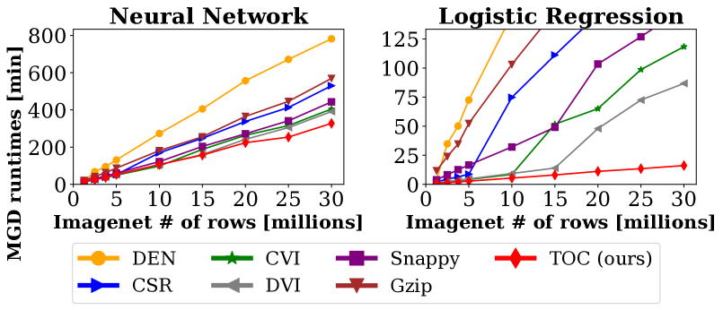
Figure 9: End-to-end MGD runtimes of ML training.

Ablation Study. We conduct an ablation study to verify whether the components in Figure 3 actually matter for TOC’s performance in reducing MGD runtimes. Specifically, we compare three variants of TOC: TOC_SPARSE (sparse encoding), TOC_SPARSE_AND_LOGICAL (sparse and logical encoding), and TOC_FULL (all the encoding techniques). Figure 10 presents the results. With more encoding techniques used, TOC’s performance becomes better, which shows the effectiveness of all our encoding components.

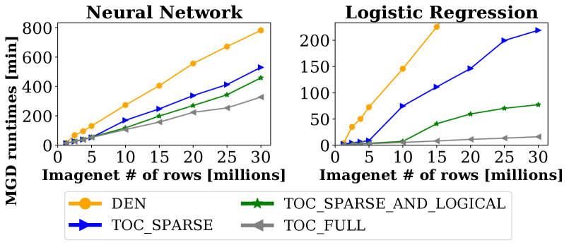
Figure 10: Ablation study of TOC for MGD runtimes.

Comparisons with Popular Machine Learning Systems. Table 6 also includes the MGD runtimes of DEN and CSR in Bismarck, ScikitLearn, and TensorFlow. We change the code of using TensorFlow and ScikitLearn a bit so that they can do disk-based learning when the dataset does not fit into memory. The table also includes BismarckTOC, which typically has less than 10 percent overhead compared with running TOC in our c++ program. This overhead is caused by the fudge factor of the database storage thus a bit larger disk IO time. On Imagenet1m and Mnist1m, BismarckTOC is comparable with the best methods in these systems (TensorFlowDEN) for NN but up to 3.2x/2.9x faster than the best methods in these systems for LR/SVM respectively. On Imagenet25m and Mnist25m, BismarckTOC is up to 2.6x/10.2x/9.8x faster than the best methods in other systems for NN/LR/SVM respectively because only the TOC data fit into memory. Thus, integrating TOC into these ML systems can greatly benefit their MGD performance.
Accuracy Study. We also plot the error rate of neural network and logistic regression as a function of time on Mnist. The goal is to compare the convergence rate of BismarckTOC with other standard tools like ScikitLearn and TensorFlow. For Mnist1m (7GB) and Mnist25m (170GB), we train 30 epochs and 10 epochs, respectively. Figure 11 presents the results. On Mnist1m and a 15GB RAM machine, BismarckTOC and TensorFlowDEN finished the training roughly at the same time, this verified our claim that BismarckTOC has comparable performance with the state-of-the-art ML system if the data fit into memory. On Mnist25m and a 15GB RAM machine, BismarckTOC finished the training much faster than other ML systems because only TOC data fit into memory. We also used a machine with 180GB RAM on Mnist25m which did not change BismarckTOC’s performance but boosted the performance of TensorFlow and ScikitLearn to be comparable with BismarckTOC as all the data fit into memory. However, renting a 180GB RAM machine is more expensive than renting a 15GB RAM machine. Thus, we believe BismarckTOC can significantly reduce users’ cloud cost.

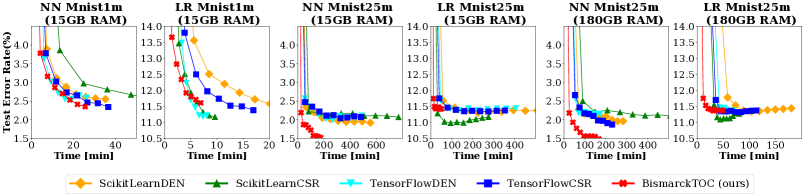
Figure 11: Test error rate on Mnist dataset as a function of time on different systems.

5.4 Compression and Decompression Runtimes

We measured the compression and decompression time of Snappy, Gzip, and TOC on mini-batches with 250 rows. The results are similar for other mini-batch sizes. Figure 12 presents the results. TOC is faster than Gzip but slower than Snappy for compression. However, TOC is faster than both Gzip and Snappy for decompression.

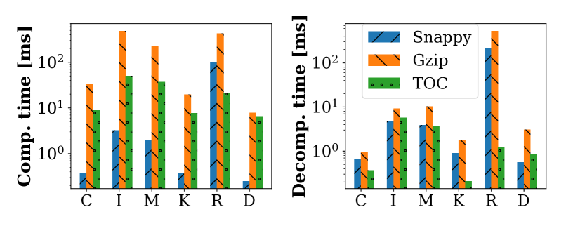
Figure 12: Left: Compression time of Snappy, Gzip and TOC on a mini-batch with 250 rows. Right: Decompression time of Snappy, Gzip, and TOC on a mini-batch with 250 rows.

6 Discussion

Advanced Neural Network. It is possible to apply TOC to more advanced neural networks such as convolutional neural networks on images. One just need to apply the common image-to-column [25] operation, which replicates the pixels of each sliding window as a matrix column. This way, the convolution operation can be expressed as the matrix multiplication operation over the replicated matrix. The replicated matrix can be compressed by TOC and we expect higher compression ratios due to the data replication.

7 Related Work

Data Compression for Analytics. There is a long line of research [1, 34, 27, 43, 14, 41] of integrating data compression into databases and relational query processing workloads on the compressed data. TOC is orthogonal to these works since TOC focuses on a different workload—mini-batch stochastic gradient descent of machine learning training.

Machine Learning Analytics Systems. There are a number of systems (e.g., MLib [29], MadLib [18], Systemml [8, 14], Bismarck [15], SimSQL [9], ScikitLearn [32], MLBase [22], and TensorFlow [2]) for machine learning workloads. Our work focuses on the algorithm perspective and is complementary to these systems, i.e., integrating TOC into these systems can greatly benefit their ML training performance.

Compressed Linear Algebra (CLA). CLA [14] compresses the whole dataset and applies batch gradient descent related operations such as vanilla BGD, L-BFGS, and conjugate gradient methods, while TOC focuses on MGD. Furthermore, CLA needs to store an explicit dictionary. When applying CLA to BGD, there are many references to dictionary entries so the dictionary cost is amortized. On a small mini-batch, there are not that many references to the dictionary entries so the explicit dictionary cost makes the CLA compression ratio less desirable. On the contrary, TOC is adapted from LZW and it does not store an explicit dictionary, so TOC achieves good compression ratios even on small mini-batches.

Factorized Learning. Factorized machine learning techniques [24, 38, 23, 11] push machine learning computations through joins and avoid the schema-based redundancy on denormalized datasets. These techniques need a schema to define the static redundancies in the denormalized datasets, while TOC can find the redundancies in the datasets automatically without a schema. Furthermore, factorized learning techniques work for BGD while TOC focuses on MGD.

8 Conclusion and Future Work

Mini-batch stochastic gradient descent (MGD) is a workhorse algorithm of modern ML. In this paper, we propose a lossless data compression scheme called tuple-oriented compression (TOC) to reduce memory/storage footprints and runtimes for MGD. TOC follows a design principle that tailors the compression scheme to the data access pattern of MGD in a way that preserves row/column boundaries in mini-batches and adapts matrix operation executions to the compression scheme as much as possible. This enables TOC to attain both good compression ratios and decompression-free executions for matrix operations used by MGD. There are a number of interesting directions for future work, including determining more workloads that can execute directly on TOC outputs and investigating the common structures between the adaptable workloads and compression schemes.

Appendix A Proof of Theorems

A.1 Theorem 1

Proof.

Without loss of generality, we use a specific row $A[i,:]$ in the proof. First, we substitute $A[i,:]$ with sequences stored in the prefix tree $\mathbf{C^{\prime}}$, then

$$A[i,:]\cdot v=\sum_{j=0}^{\mathrm{len}(\mathbf{D}[i,:])-1}\mathbf{C^{\prime}}[\mathbf{D}[i,j]].seq\cdot v$$ (9)

Plug Equation 4 into Equation 9, we get Equation 5. Following the definition of the sequence of the tree node, we immediately get Equation 6. ∎

A.2 Theorem 2

Proof.

We substitute $A$ with sequences stored in $\mathbf{C^{\prime}}$

$$v\cdot A =\sum_{i=0}^{n-1}v[i]\cdot A[i,:]$$

$$=\sum_{i=0}^{n-1}\sum_{j=0}^{\mathrm{len}(\mathbf{D}[i,:])-1}v[i]\cdot\mathbf{C^{\prime}}[\mathbf{D}[i][j]].seq.$$ (10)

Merge terms in Equation 10 with same sequences

$$v\cdot A=\sum_{i=1}^{\mathrm{len}(\mathbf{C^{\prime}})-1}\mathbf{C^{\prime}}[i].seq\cdot(\sum_{\begin{subarray}{c}\mathbf{D}[i_{k},j_{k}]=i,\forall i_{k}\in\aleph,\forall j_{k}\in\aleph\end{subarray}}v[i_{k}])$$ (11)

Plug Equation 7 into Equation 11, we get Equation 8. ∎

Appendix B More Algorithms

B.1 Right Multiplication

We present how to compute $A\cdot M,$ where $M$ is an uncompressed matrix and $A$ is a compressed matrix. This is an extension of right multiplication with vector in § 4.3.

Theorem 3.

Let $A\in\Re^{n\times m}$, $M\in\Re^{m\times p}$, D be the output of TOC on $A$, $\mathbf{C^{\prime}}$ be the prefix tree built for decoding, $\mathbf{C^{\prime}}[i].seq$ be the sequence of the tree node defined in § 3.1.1, $\mathbf{C^{\prime}}[i].key$ be the key of the tree node defined in § 4.1.2, and $\mathbf{C^{\prime}}[i].parent$ be the parent index of the tree node defined in § 4.1.2. Note that $\mathbf{C^{\prime}}[i].key$ and $\mathbf{C^{\prime}}[i].seq$ are both sparse representations of vectors (i.e., $\mathbf{C^{\prime}}[i].key\in\Re^{1\times m}$ and $\mathbf{C^{\prime}}[i].seq\in\Re^{1\times m}$). Define function $\mathcal{F}(x):\aleph\rightarrow\Re^{1\times p}$ to be

$$\mathcal{F}(x)=\mathbf{C^{\prime}}[x].seq\cdot M,x=1,2,...,\mathrm{len}(\mathbf{C^{\prime}})-1.$$ (12)

Then, we have

$$A[i,:]\cdot M= \sum_{j=0}^{\mathrm{len}(\mathbf{D}[i,:])-1}\mathcal{F}(\mathbf{D}[i][j]),i=0,1,...,n-1.$$ (13)

Proof.

Without loss of generality, we use a specific row $A[i,:]$ in the proof. First, we substitute $A[i,:]$ with sequences stored in prefix tree $\mathbf{C^{\prime}}$, then

$$A[i,:]\cdot M=\sum_{j=0}^{\mathrm{len}(\mathbf{D}[i,:])-1}\mathbf{C^{\prime}}[\mathbf{D}[i,j]].seq\cdot M$$ (14)

Plug Equation 12 into Equation 14, we get Equation 13. ∎

Algorithm 7 shows the details. First, we scan $\mathbf{C^{\prime}}$ similar to right multiplication with vector, and we use H[$i$,:] to remember the computed value of $\mathcal{F}(i)$.

Second, we scan D to compute $A\cdot M$ stored in R. For $k$th column of the result R and each D[$i$][$j$], we simply add H[D[$i$][$j$]][$k$] to R[$i$][$k$]. Because H[D[$i$][$j$]][$k$] is a random access of H, we let the loop of going over each column be the most inner loop so that we can scan D only once and have better cache performance.

Algorithm 7 Execute $A\cdot M$ on the TOC output.

1:function MatrixTimesUncompressedMatrix(D, I, $M$)

2:     inputs: column_index:value pairs in the first layer of I, encoded table D, and uncompressed matrix $M$

3:     outputs: the result of $A\cdot M$ in R

4:     $\mathbf{C^{\prime}}\leftarrow$ BuildPrefixTree(I, D)

5:     H $\leftarrow\left[0\right]$ $\triangleright$ initialize as a zero matrix

6:     for $i$ = 1 to len($\mathbf{C^{\prime}}$)-1 do $\triangleright$ scan $\mathbf{C^{\prime}}$ to compute H

7:         for $j$ = 0 to num_of_columns($M$)-1 do

8:              H[$i][j]\leftarrow\mathbf{C^{\prime}}[i].key\cdot M[:,j]+\textbf{H}[\mathbf{C^{\prime}}[i].parent][j$]               

9:     R $\leftarrow\left[0\right]$ $\triangleright$ initialize as a zero matrix

10:     for $i$ = 0 to len(D)-1 do $\triangleright$ scan D to compute R

11:         for $j$ = 0 to len(D[$i$,:])-1 do

12:              for $k$ = 0 to num_of_columns($M$)-1 do

13:                  $\textbf{R}[i][k]\leftarrow\textbf{R}[i][k]+\textbf{H}[\textbf{D}[i][j]][k]$                             

14:     return(R)

B.2 Left Multiplication

We discuss how to compute $M\cdot A$ where $M$ is an uncompressed matrix and $A$ is a compressed matrix. This is an extension of left multiplication with vector in § 4.4.

Theorem 4.

Let $A\in\Re^{n\times m}$, $M\in\Re^{p\times n}$, D be the output of TOC on $A$, $\mathbf{C^{\prime}}$ be the prefix tree built for decoding, $\mathbf{C^{\prime}}[i]$.seq be the sequence of the tree node defined in § 3.1.1, $\mathbf{C^{\prime}}[i].key$ be the key of the tree node defined in § 4.1.2, and $\mathbf{C^{\prime}}[i].parent$ be the parent index of the tree node defined in § 4.1.2. Note that $\mathbf{C^{\prime}}[i].key$ and $\mathbf{C^{\prime}}[i].seq$ are both sparse representations of vectors (i.e., $\mathbf{C^{\prime}}[i].key\in\Re^{1\times m}$ and $\mathbf{C^{\prime}}[i].seq\in\Re^{1\times m}$). Define function $\mathcal{G}(x):\aleph\rightarrow\Re^{p\times 1}$ to be

$$\mathcal{G}(x)=\sum_{\begin{subarray}{c}\mathbf{D}[i,j]=x,\forall i\in\aleph,\forall j\in\aleph\end{subarray}}M[:,i],~{}x=1,2,...,\mathrm{len}(\mathbf{C^{\prime}})-1.$$ (15)

Then, we have

$$M\cdot A= \sum_{i=1}^{\mathrm{len}(\mathbf{C^{\prime}})-1}\mathbf{C^{\prime}}[i].seq\cdot\mathcal{G}(i).$$ (16)

Proof.

We substitute $A$ with sequences stored in $\mathbf{C^{\prime}}$

$$M\cdot A =\sum_{i=0}^{n-1}M[:,i]\cdot A[i,:]$$

$$=\sum_{i=0}^{n-1}\sum_{j=0}^{\mathrm{len}(\mathbf{D}[i,:])-1}M[:,i]\cdot\mathbf{C^{\prime}}[\mathbf{D}[i][j]].seq.$$ (17)

Merge terms in Equation 17 with same sequences

$$M\cdot A=\sum_{i=1}^{\mathrm{len}(\mathbf{C^{\prime}})-1}\mathbf{C^{\prime}}[i].seq\cdot(\sum_{\begin{subarray}{c}\mathbf{D}[i_{k},j_{k}]=i,\forall i_{k}\in\aleph,\forall j_{k}\in\aleph\end{subarray}}M[:,i_{k}])$$ (18)

Plug Equation 15 into Equation 18, we get Equation 16. ∎

Algorithm 8 shows the details. First, we similarly scan D as left multiplication with vector. Specifically, we initialize $\mathbf{H}$ as a zero matrix, and then add $M[k][i]$ to $\mathbf{H}[\mathbf{D}[i][j]][k]$ for each $\mathbf{D}[i][j]$. Note that the H here is stored in transposed manner so that we only need to scan $\mathbf{D}$ once and have good cache performance at the same time.

Second, we scan $\mathbf{C^{\prime}}$ backwards to actually compute $M\cdot A$ stored in R. Specifically, for $i$th row and each $\mathbf{C^{\prime}}[j]$, we add $\mathbf{C^{\prime}}[j]$.key * $\mathbf{H}[i][j]$ to the result of $i$th row R[i,:] and add $\mathbf{H}[i][j]$ to $\mathbf{H}[i][\mathbf{C^{\prime}}[j]$.parent].

Algorithm 8 Execute $M\cdot A$ on the TOC output.

1:function UncompressedMatrixTimesMatrix(D, I, $M$)

2:     inputs: column_index:value pairs in the first layer of I, encoded table D, and uncompressed matrix $M$

3:     outputs: the result of $M\cdot A$ in R

4:     $\mathbf{C^{\prime}}\leftarrow$ BuildPrefixTree(I, D)

5:     H $\leftarrow\left[0\right]$ $\triangleright$ initialize as a zero matrix

6:     for $i$ = 0 to len(D)-1 do $\triangleright$ scan D to compute H

7:         for $j$ = 0 to len(D[$i$,:]) -1 do

8:              for $k$ = 0 to num_of_rows($M$) -1 do

9:                  $\textbf{H}[\textbf{D}[i][j]][k]\leftarrow M[k][i]+\textbf{H}[\textbf{D}[i][j]][k]$                             

10:     R $\leftarrow\left[0\right]$ $\triangleright$ initialize as a zero matrix

11:     for $i$ = len($\mathbf{C^{\prime}}$) -1 to 1 do $\triangleright$ scan $\mathbf{C^{\prime}}$ to compute R

12:         for $j$ = 0 to num_of_rows($M$) -1 do

13:              $\textbf{R}[j,:]\leftarrow\textbf{R}[j,:]+\mathbf{C^{\prime}}[i]$.key * $\textbf{H}[i][j]$

14:              Add $\textbf{H}[i][j]$ to $\textbf{H}[\mathbf{C^{\prime}}[i]$.parent$][j]$               

15:     return(R)

Appendix C More Time Complexity Analysis

Executing $M\cdot A$ and $A\cdot M$ needs to build $\mathbf{C^{\prime}}$, scan $\mathbf{C^{\prime}}$, and scan D. As shown in Algorithm 2, building $\mathbf{C^{\prime}}$ has complexity $\mathcal{O}(|\mathbf{I}|+|\mathbf{D}|)$ and $|\mathbf{C^{\prime}}|=|\mathbf{I}|+|\mathbf{D}|$. When scanning $\mathbf{C^{\prime}}$ and $\mathbf{D}$, each element needs to do r$ow\_size(\mathbf{M})/col\_size(\mathbf{M})$ operations for $M\cdot A$/$A\cdot M$ respectively. Thus, the time complexity for $M\cdot A$ and $A\cdot M$ is $\mathcal{O}(row\_size(\mathbf{M})*(|\mathbf{I}|+|\mathbf{D}|))$ and $\mathcal{O}(col\_size(\mathbf{M})*(|\mathbf{I}|+|\mathbf{D}|))$ respectively.

Appendix D More Experiments

D.1 Integration TOC into Bismarck

We integrated TOC into Bismarck and replaced its existing matrix kernels. There are three key parts of the integration. First, we allocate an arena space in Bismarck shared memory for storing the ML models. Second, we replace the existing Bismarck matrix kernel with the TOC matrix kernel for updating the ML models. Third, a database table is used to store the TOC compressed mini-batches and the serialized bytes of each TOC compressed mini-batch are stored as a bytes field of variable length in the row. After all these, we modified the UDF of ML training to read the compressed mini-batch from the table and use the replaced matrix kernel to update the ML model in the arena.

Table 7: End-to-end MGD runtimes (in minutes) for training machine learning models: Neural network(NN), Logistic regression (LR), and Support vector machine (SVM) on datasets Census and Kdd99. Census15m and Census290m is 7GB and 140GB respectively, while Kdd7m and Kdd200m is 7GB and 200GB respectively.

Methods	Census15m			Census290m			Kdd7m			Kdd200m
	NN	LR	SVM	NN	LR	SVM	NN	LR	SVM	NN	LR	SVM
TOC (ours)	35	0.8	0.7	702	16	14	16.1	0.2	0.2	323	6.1	5.9
DEN	39	4.0	4.0	1108	253	251	29	4.6	4.4	1003	608	615
CSR	38	1.8	1.8	942	161	167	19.2	0.4	0.4	438	56	53
CVI	37	1.1	1.0	844	80	67	18.5	0.3	0.3	422	31	30
DVI	38	1.2	1.1	800	46	43	28.4	1.2	1.1	611	71	71
Snappy	41	4.7	4.6	905	121	115	27.2	3.5	3.5	616	127	128
Gzip	46	11.1	11.1	965	244	241	33.5	7.5	7.5	683	235	235
BismarckTOC	38	0.87	0.88	742	17.4	14.8	16.8	0.3	0.31	329	6.4	6.3
BismarckDEN	N/A	4.2	4.3	N/A	321	310	N/A	4.0	3.8	N/A	645	644
BismarckCSR	N/A	3.2	3.2	N/A	222	234	N/A	0.9	0.9	N/A	114	115
ScikitLearnDEN	73.2	7.3	6.6	1715	604	580	42	5	4.6	1797	771	772
ScikitLearnCSR	105.1	5.7	5.1	2543	421	408.8	44	1.7	1.5	1476	166	160
TensorFlowDEN	38.1	9.4	10.5	1073	638	610	21.4	5.5	5.1	1199	781	779
TensorFlowCSR	54.7	15.1	14.0	1244	681	661	15.2	4.1	4.4	577	300	274

D.2 End-to-End MGD Runtimes

MGD runtimes on Census and Kdd99 are reported in Table 7. Overall, the results are similar to those presented in § 5.3. On small datasets like Census15m and Kdd7m, TOC has comparable performance with other methods. On large datasets like Census290m and Kdd200m, TOC is up to 1.8x/17.8x/18.3x faster than the state-of-the-art compression schemes for NN/LR/SVM respectively. We leave the results of datasets Rcv1 and Deep1Billion because of their extreme sparsity/density such that we do not expect better performance from TOC.

References

- [1] D. Abadi, S. Madden, and M. Ferreira. Integrating compression and execution in column-oriented database systems. In Proceedings of the 2006 ACM SIGMOD international conference on Management of data, pages 671–682. ACM, 2006.
- [2] M. Abadi et al. Tensorflow: A system for large-scale machine learning. In OSDI, volume 16, pages 265–283, 2016.
- [3] M. Amini, N. Usunier, and C. Goutte. Learning from multiple partially observed views-an application to multilingual text categorization. In Advances in neural information processing systems, pages 28–36, 2009.
- [4] A. Ashari et al. On optimizing machine learning workloads via kernel fusion. In ACM SIGPLAN Notices, volume 50, pages 173–182. ACM, 2015.
- [5] A. Babenko and V. Lempitsky. Efficient indexing of billion-scale datasets of deep descriptors. In Proceedings of the IEEE Conference on Computer Vision and Pattern Recognition, pages 2055–2063, 2016.
- [6] Y. Bengio. Practical recommendations for gradient-based training of deep architectures. In Neural networks: Tricks of the trade, pages 437–478. Springer, 2012.
- [7] G. E. Blelloch. Introduction to data compression. Computer Science Department, Carnegie Mellon University, 2001.
- [8] M. Boehm et al. Hybrid parallelization strategies for large-scale machine learning in systemml. Proceedings of the VLDB Endowment, 7(7):553–564, 2014.
- [9] Z. Cai et al. Simulation of database-valued markov chains using simsql. In Proceedings of the 2013 ACM SIGMOD International Conference on Management of Data, pages 637–648. ACM, 2013.
- [10] C. Chelba et al. One billion word benchmark for measuring progress in statistical language modeling. arXiv preprint arXiv:1312.3005, 2013.
- [11] L. Chen et al. Towards linear algebra over normalized data. Proceedings of the VLDB Endowment, 10(11):1214–1225, 2017.
- [12] J. Dean. Challenges in building large-scale information retrieval systems: invited talk. In Proceedings of the Second ACM International Conference on Web Search and Data Mining, pages 1–1. ACM, 2009.
- [13] J. Dean et al. Large scale distributed deep networks. In Advances in neural information processing systems, pages 1223–1231, 2012.
- [14] A. Elgohary et al. Compressed linear algebra for large-scale machine learning. Proceedings of the VLDB Endowment, 9(12):960–971, 2016.
- [15] X. Feng et al. Towards a Unified Architecture for in-RDBMS Analytics. In Proceedings of the 2012 ACM SIGMOD International Conference on Management of Data, pages 325–336. ACM, 2012.
- [16] S. Garavaglia and A. Sharma. A smart guide to dummy variables: Four applications and a macro. In Proceedings of the Northeast SAS Users Group Conference, page 43, 1998.
- [17] D. Harnik et al. Estimation of deduplication ratios in large data sets. In Mass Storage Systems and Technologies (MSST), 2012 IEEE 28th Symposium on, pages 1–11. IEEE, 2012.
- [18] J. M. Hellerstein et al. The madlib analytics library: or mad skills, the sql. Proceedings of the VLDB Endowment, 5(12):1700–1711, 2012.
- [19] G. Hinton, N. Srivastava, and K. Swersky. Neural networks for machine learning lecture 6a overview of mini-batch gradient descent. Cited on, page 14, 2012.
- [20] Z. Kaoudi et al. A cost-based optimizer for gradient descent optimization. In Proceedings of the 2017 ACM International Conference on Management of Data, pages 977–992. ACM, 2017.
- [21] K. Kourtis, G. Goumas, and N. Koziris. Optimizing sparse matrix-vector multiplication using index and value compression. In Proceedings of the 5th conference on Computing frontiers, pages 87–96. ACM, 2008.
- [22] T. Kraska et al. Mlbase: A distributed machine-learning system. In Cidr, volume 1, pages 2–1, 2013.
- [23] A. Kumar et al. To join or not to join? thinking twice about joins before feature selection. In Proceedings of the 2016 International Conference on Management of Data, pages 19–34. ACM, 2016.
- [24] A. Kumar, J. Naughton, and J. M. Patel. Learning generalized linear models over normalized data. In Proceedings of the 2015 ACM SIGMOD International Conference on Management of Data, pages 1969–1984. ACM, 2015.
- [25] L. Lai, N. Suda, and V. Chandra. Cmsis-nn: Efficient neural network kernels for arm cortex-m cpus. arXiv preprint arXiv:1801.06601, 2018.
- [26] D. Lemire and L. Boytsov. Decoding billions of integers per second through vectorization. Software: Practice and Experience, 45(1):1–29, 2015.
- [27] Y. Li and J. M. Patel. Bitweaving: fast scans for main memory data processing. In Proceedings of the 2013 ACM SIGMOD International Conference on Management of Data, pages 289–300. ACM, 2013.
- [28] M. Lichman. UCI machine learning repository, 2013.
- [29] X. Meng et al. Mllib: Machine learning in apache spark. The Journal of Machine Learning Research, 17(1):1235–1241, 2016.
- [30] D. Mishkin, N. Sergievskiy, and J. Matas. Systematic evaluation of cnn advances on the imagenet. arXiv preprint arXiv:1606.02228, 2016.
- [31] F. Niu et al. Hogwild: A lock-free approach to parallelizing stochastic gradient descent. In NIPS, 2011.
- [32] F. Pedregosa et al. Scikit-learn: Machine learning in Python. Journal of Machine Learning Research, 12:2825–2830, 2011.
- [33] C. Qin, M. Torres, and F. Rusu. Scalable asynchronous gradient descent optimization for out-of-core models. Proceedings of the VLDB Endowment, 10(10):986–997, 2017.
- [34] V. Raman et al. Db2 with blu acceleration: So much more than just a column store. Proceedings of the VLDB Endowment, 6(11):1080–1091, 2013.
- [35] S. Ruder. An overview of gradient descent optimization algorithms. arXiv preprint arXiv:1609.04747, 2016.
- [36] O. Russakovsky et al. Imagenet large scale visual recognition challenge. International Journal of Computer Vision, 115(3):211–252, 2015.
- [37] Y. Saad. Iterative methods for sparse linear systems, volume 82. siam, 2003.
- [38] M. Schleich, D. Olteanu, and R. Ciucanu. Learning linear regression models over factorized joins. In Proceedings of the 2016 International Conference on Management of Data, pages 3–18. ACM, 2016.
- [39] S. Shalev-Shwartz and S. Ben-David. Understanding Machine Learning: From Theory to Algorithms. Cambridge University Press, 2014.
- [40] S. Shalev-Shwartz et al. Learnability, stability and uniform convergence. The Journal of Machine Learning Research, 11:2635–2670, 2010.
- [41] J. Wang et al. An experimental study of bitmap compression vs. inverted list compression. In Proceedings of the 2017 ACM International Conference on Management of Data, pages 993–1008. ACM, 2017.
- [42] T. A. Welch. A technique for high-performance data compression. Computer, 6(17):8–19, 1984.
- [43] R. M. G. Wesley and P. Terlecki. Leveraging compression in the tableau data engine. In Proceedings of the 2014 ACM SIGMOD international conference on Management of data, pages 563–573. ACM, 2014.
- [44] R. H. Wiggins et al. Image file formats: Past, present, and future 1. Radiographics, 21(3):789–798, 2001.
- [45] X. Wu et al. Bolt-on differential privacy for scalable stochastic gradient descent-based analytics. In Proceedings of the 2017 ACM International Conference on Management of Data, pages 1307–1322. ACM, 2017.
- [46] H.-F. Yu et al. Large linear classification when data cannot fit in memory. ACM Transactions on Knowledge Discovery from Data (TKDD), 5(4):23, 2012.
- [47] J. Ziv and A. Lempel. A universal algorithm for sequential data compression. IEEE Transactions on information theory, 23(3):337–343, 1977.
- [48] J. Ziv and A. Lempel. Compression of individual sequences via variable-rate coding. IEEE transactions on Information Theory, 24(5):530–536, 1978.