Abstract

This note discusses methods of particle reconstruction in the forward region detectors of future $\mathup{{{\mathup{{{e}}}}}^{\scriptstyle{+}}}$ $\mathup{{{\mathup{{{e}}}}}^{\scriptstyle{-}}}$ linear colliders such as ILC or CLIC. At the nominal luminosity the innermost electromagnetic calorimeters undergo high particle fluxes from the beam-induced background. In this prospect, different methods of the background simulation and signal electron reconstruction are described.

1 Introduction

The future TeV energy range $\mathup{{{\mathup{{{e}}}}}^{\scriptstyle{+}}}$ $\mathup{{{\mathup{{{e}}}}}^{\scriptstyle{-}}}$ colliders (ILC [1], CLIC [2]) are expected to become sensitive probes for potential new physics processes or at least significantly contribute to the validation of the Standard Model (SM). Many Beyond Standard Model (BSM) searches have $t$-channel SM processes as a background [3], the rejection of this background motivates detector fiducial coverage down to the smallest possible polar angles.

The BeamCal detector system [4] is centred around the outgoing beam axis in the forward direction. Its purposes are: tagging of high energy electrons to suppress backgrounds to potential BSM process, shielding of the accelerator components from the beam-induced background, and providing supplementary beam diagnostics information extracted from the pattern of incoherent-pair energy depositions in the BeamCal [5].

To achieve nominal luminosities at the level of ${10}^{34}\text{\,}\mathrm{c}\mathrm{m}^{-2}\mathrm{s}^{-1}$, nanometre-sized beams are necessary. The high charge density in the bunches will induce strong electromagnetic fields causing deflection of the beam particles and the radiation of beamstrahlung. In addition, the beamstrahlung photons will interact with the beam particles and produce electron–positron and quark–anti-quark pairs. While the photonic component will be radiated practically along the outgoing beam axis, a noticeable fraction of leptonic and hadronic pairs will hit the BeamCal calorimeter in the forward region. The distribution of energy depositions from incoherent pairs depends on the beam parameters and shape and strength of the detector magnetic field.

Electron tagging at low angles is thus complicated by the high occupancy in the BeamCal [6]. The reconstruction software for the forward region must include a background-adaptive algorithm in order to provide maximum tagging efficiency for high energy final state electrons produced in the collisions.

In this note two such algorithms are presented and have their performance studied. The first algorithm implements clusterization of signal energy depositions in the calorimeter shower. The second method is based on fitting the laterally projected energy distribution with an analytical formula describing shower energy deposition. The approaches to the background simulation are also reviewed.

Besides the electron tagging algorithms, the reconstruction software has several features. It is usable for different detector geometries which can be defined in the configuration files. It allows tuning of the reconstruction parameters and presents a choice of several background simulation options. The code extensibility makes it technically possible for users to implement their own electron tagging algorithm.

The note is structured as follows: the BeamCal detector design is briefly described in Section 2, Section 3 contains a description of beam-induced background treatment in the simulation and Section 4 presents two methods of high energy electron reconstruction in the BeamCal, the algorithm performance and background methods are compared in Section 5, Section 6 contains the summary of this study, the tool for background conversion and the list of simulation options are described in Appendix A and Appendix B, respectively.

2 BeamCal Detector

The BeamCal is a tungsten-sandwich sampling calorimeter centred on the outgoing beam-axis. The large dose imparted by the beam-induced backgrounds requires the use of radiation hard sensors.

The choice of the segmentation for the BeamCal sensors influences the reconstruction efficiency. Figure 1 shows two different possible segmentations for the BeamCal: uniform and proportional. In the uniform type of segmentation the pads have approximately the same size. This type of design is used in the current studies. In this case the reconstruction efficiency degrades with lower radii where the background occupancy is higher. An alternative proportional segmentation without this drawback can be used, but requires further developments of the simulation.

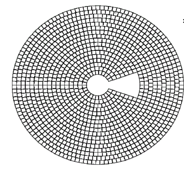
(a)

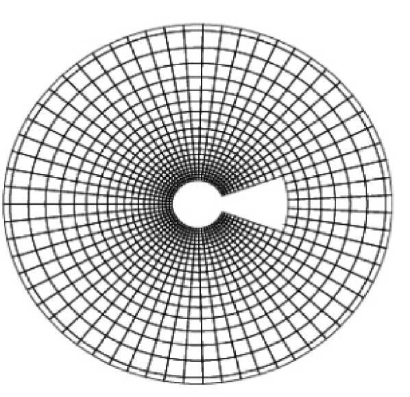
(b)

Figure 1: Different segmentation schemes for the BeamCal calorimeter: uniform 1(a) and proportional 1(b).

In the CLIC_ILD_CDR [7] geometry used for current studies the BeamCal detector has 40 layers of $3.5\text{\,}\mathrm{m}\mathrm{m}$ thick tungsten absorber and radiation-resistant $0.3\text{\,}\mathrm{m}\mathrm{m}$ sensor uniformly segmented into approximately $8\times$$8\text{\,}\mathrm{m}\mathrm{m}^{2}$ pads. The R&D studies to select the sensor material most suitable for hard radiation environment are ongoing [8, 9] and the current Geant4 simulation uses diamond sensors. Figure 2 shows a render of simulated calorimeter with a $100\text{\,}\mathrm{m}\mathrm{m}$ graphite shield to absorb particles backscattered in the direction of IP. The described BeamCal geometry covers the polar angle span from $10\text{\,}\mathrm{m}\mathrm{r}\mathrm{a}\mathrm{d}$ to $43\text{\,}\mathrm{m}\mathrm{r}\mathrm{a}\mathrm{d}$.

The possibility of adjustable geometry and segmentation is accounted for in the reconstruction framework.

Figure 2: The BeamCal in a CLIC detector model. Shown is the beam pipe, the BeamCal, and the kicker and beam position monitor of the intra-train-feedback system. The Z position is given with respect to the interaction point, the radial dimension is relative to the outgoing beam axis.

3 Simulation of the Beam-induced Background

In the current setup the simulated BeamCal event consists of the energy depositions from signal events and the energy from the background sample. For simplicity and computational efficiency the signal and background processes are generated and simulated separately.

To provide the incoherent pair background for the BeamCal reconstruction four methods were implemented. For each of the background generation methods a set of simulated background bunch crossings are required as a basis. From this background pool complete bunch crossings are used during the reconstruction. Alternatively, distributions and parametrisations derived from the background pool can be used. The procedure to select the background method and set the number of bunch crossings in the configuration file is described in the Appendix B.

3.1 Pregenerated Background

The first method uses a Monte Carlo technique and is named ‘pregenerated’. The event background sample is constructed from the corresponding number of bunch crossings occurring within the read-out time window randomly selected from the background pool. This method gives the most precise and realistic description of the background. However, the background pool – consisting of hundreds of bunch crossings – has to be provided during the reconstruction. This approach is useful to estimate the BeamCal reconstruction efficiency, but the total file sizes can be prohibitive for large scale Monte Carlo campaigns.

The procedure to convert a simulated bunch crossing into the background root file is described in Appendix A.

3.2 Parametrised Background

An alternative method of providing the energy deposition in the BeamCal by background particles is called ‘parametrised’, where the background energy deposition in each pad is generated according to the distribution

$$F(x)=\frac{A}{x}\exp{\left(\frac{x-B}{C}\right)}^{2}$$

where the $A,B$ and $C$ parameters are determined for each pad by fitting the energy depositions from the background pool. An example of background energy distributions for three selected pads is shown with the corresponding fitted functions on Figure 3. The pads were selected to represent three distinct energy spectra: pad #1 in Figure 3(a) with a quasi-symmetric Gaussian, pad #2 in Figure 3(b) with a Gaussian near 0 and pad #3 in Figure 3(c) with lower energy depositions proportional to $1/x$. The pad positions are marked on the front view of the first sensor plane in Figure 3(d). All three sample spectra are reasonably well described by the provided parametrization.

(a)

(b)

(c)

(d)

Figure 3: 3(a)–3(c) The distribution of the background energy deposition for bunch crossings at $3\text{\,}\mathrm{TeV}$ CLIC in three distinct pads fitted with the parametrisation. 3(d) The corresponding pads marked at the BeamCal front projection of layer 10. The plots show that different background energy spectra are well described by the same parametrisation.

The parametrised method gives a result that is almost as precise as the ‘pregenerated’ method except for the correlations between the energy deposits in neighbouring pads. The plot in Figure 4(a) shows the correlation matrix between the 120 innermost pads in the front projection representing the area with the highest energy deposition (the first three rings). The correlation matrix on Figure 4(b) is drawn for one of the innermost towers of pads along the detector axis. The plots show that the correlations are small in most parts of the detector and especially in the region normally used for the reconstruction (after the tenth layer). The correlations can therefore be neglected for the parametrised and the Gaussian methods of the background generation.

(a)

(b)

Figure 4: Background energy deposition correlations between pads in three inner rings of the $10^{\mathrm{th}}$ layer 4(a) and along the BeamCal axis for one of the innermost pads 4(b). The corresponding pad or layer numbers are given along the axes. The backgrounds are for CLIC at $3\text{\,}\mathrm{TeV}$.

Due to the large number of pads in the BeamCal the generation time becomes very long for a large number of bunch crossings. This method is thus applicable for cases where only a few bunch crossings take place within the read-out time window.

The procedure to convert a simulated bunch crossing into the background file usable with this and the Gaussian approach is described in Appendix A.

3.3 Gaussian Background

Another method of producing background is called ‘Gaussian’, where the background energy deposition in each pad is generated according to a Gaussian distribution with a mean of $\bar{E}_{\mathrm{Pad}}$ and a variance $\sigma_{\mathrm{Pad}}^{2}$ determined from the background pool. Although for single bunch crossings the distribution of energy deposition in a pad differs from a Gaussian distribution, for sufficiently large number of bunch crossings $N>10$ the distribution of their sum will be well described by a Gaussian with the mean $N\bar{E}_{\mathrm{Pad}}$ and the variance $N\sigma_{\mathrm{Pad}}^{2}$, according to the Central Limit Theorem. This method is thus applicable for the read-out samples over a large number of bunch crossings.

3.4 Averaged Background

The fourth possibility is similar to using the Gaussian background. The method is provided in the simulation for backward compatibility with the electron tagging reconstruction in MarlinReco [10] and can read the files with averaged energy density used in that processor. The background distribution is generated from the averages.

4 High Energy Electron Reconstruction

The techniques of shower position reconstruction in laterally segmented calorimeters were developed and presented in [11, 12, 13]. They essentially converge to two methods: a clustering algorithm based on calculation of the centre of gravity of signal pads, previously used in the FCal collaboration [14]; and a method based on fitting the energy deposition with a modelled shower shape. While the first method is simpler and faster, it is optimised for perpendicularly segmented sensors. In case of the radial segmentation, the fitting method may have better performance in terms of precision. However the main purpose of the BeamCal detector is the tagging of high-energy electrons, while measuring their spatial coordinates has lower priority. Therefore the choice between these methods will have to be made depending on the specific application or analysis.

To perform electron tagging with the BeamCal a reconstruction procedure was developed. It relies on the two aforementioned algorithms implemented as a Marlin [15] processor BeamCalClusterReco and built into the global detector reconstruction framework. The processor also takes care of background generation when the reconstruction is applied to simulated signal.

4.1 Clustering Algorithm

This clustering option is a nearest neighbour search based on the pads with significant remaining energy after the subtraction of the average background.

4.1.1 Energy Subtraction

In the first step of the algorithm the average expected energy from incoherent pair background $\vec{E}^{\mathrm{Average}}$ is removed from the total energy $\vec{E}^{\mathrm{Event}}_{\mathrm{Total}}$, which is the sum of the signal and background energy deposits for each pad. Given the remaining energy in each pad,

$$\vec{E}^{\mathrm{Event}}_{\mathrm{Remaining}}=\vec{E}^{\mathrm{Event}}_{\mathrm{Total}}-\vec{E}^{\mathrm{Average}},$$

pads for clusters are selected.

4.1.2 Pad Selection

As the next step, pads with a significant amount of remaining energy are chosen for the clustering. There are two options to select pads. A pad selection based on a constant minimal required energy depending on the ring of a pad, and a pad selection based on the standard deviation of the background energy deposit in each pad.

Constant Energy Selection

A pad is selected for further clustering if the pad energy $E_{\mathrm{Pad}}(\mathrm{Ring}_{\mathrm{Pad}})$ is larger than the minimal required energy in its ring $E^{\mathrm{Cut}}_{\mathrm{Pad}}(\mathrm{Ring}_{\mathrm{Pad}})$

$$E_{\mathrm{Pad}}(\mathrm{Ring}_{\mathrm{Pad}})>E^{\mathrm{Cut}}_{\mathrm{Pad}}(\mathrm{Ring}_{\mathrm{Pad}})\,.$$

The pad selection in this case is steered by the ETPad parameter of the BeamCalReco processor.

Variable Energy Selection

In this case, pads are selected based on the energy fluctuation of the background from event to event. The standard deviation of the energy fluctuations for the background $\sigma^{\mathrm{Pad}}_{\mathrm{BKG}}$ is calculated. Pads are selected if the remaining energy $E_{\mathrm{Pad}}$ is larger than $N_{\sigma}$ standard deviations. It is also possible to define a minimal remaining energy $E^{\mathrm{Cut}}_{\min}$ to select only pads which have at least $E^{\mathrm{Cut}}_{\min}$ remaining energy

$$E_{\mathrm{Pad}}>\max(E^{\mathrm{Cut}}_{\min},\,N_{\sigma}\cdot\sigma^{\mathrm{Pad}}_{\mathrm{BKG}})\,.$$

In the processor parameters, $E^{\mathrm{Cut}}_{\min}$ is equal to the first value of the ETPad parameter and $N_{\sigma}$ is given by the SigmaCut parameter.

4.1.3 Tower Creation and Nearest Neighbour Search

From the selected pads towers are created. A tower is simply the collection of pads with the same r and $\phi$ coordinates in the BeamCal. The tower with the largest number of selected pads is chosen. The pads in a tower do not have to be in consecutive layers. If there are towers next to the primary towers, these are added to the primary tower, and the added towers are also checked for neighbours. Finally, a cluster is created from the tower if there are more than MinimumTowerSize pads in the cluster. If there are towers not included in this first cluster, additional clusters might be created until no more towers remain.

4.1.4 Cluster Location Calculation

The tower locations are calculated based on the energy-weighted position of the pads in each tower.

The polar angle $\theta_{\mathrm{Reco}}$ is calculated from the average ring $R_{\mathrm{Cluster}}$ of the cluster, where $R_{\mathrm{Pad}}$ is the radius of a pad

$$R_{\mathrm{Cluster}}= \frac{1}{E_{\mathrm{Cluster}}}\sum_{\mathrm{Pads}}E_{\mathrm{Pad}}\,R_{\mathrm{Pad}}\,;$$

and the azimuthal angle

$$\phi_{\mathrm{Cluster}}= \mathrm{ATan2}\left(\frac{1}{E_{\mathrm{Cluster}}}\sum_{\mathrm{Pads}}E_{\mathrm{Pad}}\sin{\phi_{\mathrm{Pad}}},\qquad\frac{1}{E_{\mathrm{Cluster}}}\sum_{\mathrm{Pads}}E_{\mathrm{Pad}}\cos{\phi_{\mathrm{Pad}}}\right),$$

are calculated from the energy weighted azimuthal angle $\phi_{\mathrm{Pad}}$ of the pads in the cluster, where the sums are the average position in $Y$ and $X$, and $\mathrm{ATan2}$ is the two-argument arc-tangent function commonly found in mathematical libraries.

4.2 Shower Fitting Algorithm

This approach is based on approximating the profile of the high energy electron shower with a two-dimensional exponential distribution. The algorithm utilises a $\chi^{2}$-test to detect an excess in the energy deposition over the background. In the present case, i.e., in simulation, the average background value and its variance are extracted from the background pool. The event sample with its total energy deposition is constructed as described in Section 3. The reconstruction is performed within a subset of calorimeter layers which is defined with a starting layer and depth parameters in the configuration file.

4.2.1 Step 1

The energy depositions in the layers are projected along the calorimeter axis to its front plane. Each pad in the resulting front projection contains the following quantities, where the summation is performed over pads in the layers:

• sum of the total energy depositions behind the pad,

  $$E_{\mathrm{proj}}^{\mathrm{tot}}=\sum E_{\mathrm{Pad}}^{\mathrm{tot}}\,;$$

• sum of the average background depositions,

  $$\bar{E}_{\mathrm{proj}}^{\mathrm{bkg}}=\sum\bar{E}_{\mathrm{Pad}}^{\mathrm{bkg}}\,;$$

• sum of the background variance,

  $$\sigma^{2}_{\mathrm{proj}}=\sum\sigma^{2}_{\mathrm{Pad}}\,;$$

• quadratic norm,

  $$\chi^{2}_{\mathrm{proj}}=\sum\frac{{(E_{\mathrm{Pad}}^{\mathrm{tot}}-\bar{E}_{\mathrm{Pad}}^{\mathrm{bkg}})}^{2}}{\sigma^{2}_{\mathrm{Pad}}}\,.$$

4.2.2 Step 2

After the values are calculated, the algorithm tries to form a shower spot. It selects a pad from the projection satisfying the following criteria:

• the pad has the highest $\chi^{2}_{\mathrm{proj}}$ and it is above a configured threshold $\chi^{2}_{\mathrm{\mathrm{proj},\min}}$;

• the difference $E_{\mathrm{proj}}^{\mathrm{tot}}-\bar{E}_{\mathrm{proj}}^{\mathrm{bkg}}$ is above 70% of the configured energy threshold for the total shower energy $E_{\mathrm{min}}$ defined by the ETCluster parameter and described in Appendix B.

The selected pad is declared the central pad of the shower. Other pads within $2\rho_{M}$ (Moliere radius) are inspected for the following criteria:

• the difference $E_{\mathrm{proj}}^{\mathrm{tot}}-\bar{E}_{\mathrm{proj}}^{\mathrm{bkg}}$ is above 10% of the configured energy threshold for the total shower energy $E_{\mathrm{min}}$ defined by the ETCluster parameter (see Appendix B);

• the signal energy measured in standard deviations of the background $(E_{\mathrm{proj}}^{\mathrm{tot}}-\bar{E}_{\mathrm{proj}}^{\mathrm{bkg}})/\sigma_{\mathrm{proj}}$ is $>1$.

Such pads are added as peripheral pads to the spot.

4.2.3 Step 3

For simplicity, the shower transverse energy distribution is approximated with

$$E(r)=E_{0}\exp\left(-\frac{r}{R_{0}}\right)\,,$$

where $r$ is the distance from the shower centre, $E_{0}$ is a scaling factor and $R_{0}$ is the shower width. The shower width varies with its depth so that $R_{0}$ depends on the layers from which the energy projection is calculated.

The fit is performed with four parameters: the shower centre coordinates $R$ and $\phi$ in the polar coordinate system with the origin placed at the BeamCal centre, the scaling coefficient $E_{0}$, and the shower width $R_{0}$. Initial values of the centre coordinates are estimated with the centre-of-gravity method with logarithmic weights [13]. Using numeric integration the algorithm calculates approximate energy deposition in each spot pad $E_{\mathrm{int}}$ and calculates a $\chi^{2}$ measure:

$$\chi^{2}_{\mathrm{spot}}=\sum_{\mathrm{spot\;pads}}\frac{{(E^{\mathrm{int}}-(E_{\mathrm{proj}}^{\mathrm{tot}}-\bar{E}_{\mathrm{proj}}^{\mathrm{bkg}}))}^{2}}{\sigma^{2}_{\mathrm{proj}}}\,,$$

MINUIT [16] is then used to minimise this value by varying the $R,\phi,E_{0}$ and $R_{0}$ parameters. The resulting $R$ and $\phi$ values are treated as the shower centre and the $E^{\mathrm{int}}$ value corresponding to the minimum $\chi^{2}_{\mathrm{spot}}$ as the shower energy.

4.2.4 Step 4

Steps 2 and 3 are repeated with the next shower candidate until no more candidates are found in the front projection.

5 Algorithm Performance

The two algorithms presented in the previous section were compared in terms of efficiency, fake rate, and spatial and energy resolution. The tests were performed with beam-induced background simulated for $3\text{\,}\mathrm{TeV}$ collisions and signal samples with electron energies from $500\text{\,}\mathrm{G}\mathrm{e}\mathrm{V}$ to $1500\text{\,}\mathrm{GeV}$. The beam energy of $1.5\text{\,}\mathrm{TeV}$ corresponds to the highest and most challenging background occupancy in the BeamCal. Two methods of background generation were tested: pregenerated and Gaussian. In the reconstruction the read-out window was set to $40\text{\,}\mathrm{B}\mathrm{X}$ which means that every signal event was overlaid with background energy deposition accumulated during 40 bunch crossings.

To test the selection efficiency, mono-energetic electrons and incoherent pair background were simulated separately in the Geant4-based Mokka framework [17]. For the incoherent pair background at the $3\text{\,}\mathrm{TeV}$ CLIC, beam-beam interactions with irregular beam shapes were simulated with the GuineaPig Monte Carlo program [18]. Each element of the background collection corresponds to a single bunch crossing (BX) with different random seeds and different initial beam-particle distributions.

To produce an event for the analysis sample the signal energy deposition ($E^{\mathrm{signal}}$) was overlaid on top of the incoherent pair background ($E^{\mathrm{bkg}}$) which would accumulate within the read-out window.

The algorithm performance is demonstrated by efficiency plots shown in Figure 5 for different combinations of reconstruction (clustering and shower fitting) and background simulation methods (pregenerated and Gaussian). The fraction of detected electrons depends on their energy and polar angle with respect to the detector axis. At lower $\theta$, the background occupancy is high and therefore the efficiency is lower.

(a)

(b)

Figure 5: Polar angle dependence of the reconstruction efficiency for different methods. Efficiency for 5(a) $500\text{\,}\mathrm{GeV}$ and 5(b) $1500\text{\,}\mathrm{GeV}$ electrons hitting BeamCal.

The quality of the reconstruction was compared for three cases: clustering algorithm with pregenerated background and shower fitting algorithm with pregenerated and Gaussian backgrounds. In order to perform the comparison the configurations were optimized to obtain fake rates at approximately the same value of 5%, as shown in Figure 6. To obtain equal fake rates the shower fitting algorithm parameter TowerChi2ndfLimit was set to 5.5 for pregenerated background and 1.86 for Gaussian background, while the clusterization algorithm parameters were set to their defaults.

A reconstructed cluster was considered to be a fake electron if it differs by more than $5\text{\,}\mathrm{mrad}$ in $\theta$ and if the $\sin$ and $\cos$ of the azimuthal angle differ by more than 0.35 with respect to the generated particle. The energy of the reconstructed cluster was required to be above the configured threshold as well. Because the fake rate only depends on the selection criteria and the background, it is independent of the incident electron energy.

Figure 6: Dependence of the reconstruction fake rate on the incident electron energy.

Figure 7 shows a resolution comparison for the two algorithms as a function of the energy of the signal electron. The resolution is defined as the standard deviation of the difference between the measured quantity and the original value taken from the generator level. With the configuration described above, the polar angle resolution is in the range of $0.250.4\text{\,}\mathrm{mrad}$ for the clustering-based algorithm and $0.20.3\text{\,}\mathrm{mrad}$ for the shower fitting approach. For the reconstruction of the azimuthal angle, the clustering method gives an average of $1.2\mathrm{°}$ and the shower fitting method an average of $0.5\mathrm{°}$. In both cases the resolution increases with higher electron energy. As expected, the fitting algorithm being properly adjusted shows better resolution than the clustering algorithm. The choice of the background simulation has a negligible effect on the angular resolution.

(a)

(b)

Figure 7: Angular resolution of reconstructed electrons for different reconstruction and background simulation methods as a function of the electron energy for the polar 7(a) and azimuthal 7(b) angle.

The energy resolution is defined as the ratio of the standard deviation of the reconstructed cluster or shower energy to its average. The resolution is shown in Figure 8. The plot shows that the shower fitting algorithm provides approximately 20% better energy resolution than the clustering algorithm. There is little sensitivity to the background generation method. In all cases the resolution improves with higher electron energies.

Figure 8: Energy resolution of reconstructed electrons for different reconstruction and background simulation methods as a function of the electron energy.

6 Summary

A dedicated study of the reconstruction of high-energy electrons in the BeamCal detector at CLIC and ILC is presented. The forward detector regions at these future $\mathup{{{\mathup{{{e}}}}}^{\scriptstyle{+}}}$$\mathup{{{\mathup{{{e}}}}}^{\scriptstyle{-}}}$ colliders will be exposed to high particle fluxes from beam-induced background. This imposes constraints on the detection of signal particles at small polar angles and requires optimised background simulation as well as reconstruction algorithms.

To realistically approximate the reconstruction of high energy electrons in the forward region a reconstruction package for the Marlin framework was developed. It creates background distributions and reconstructs showers in the BeamCal.

Four different methods to create background distributions were implemented and compared: using pregenerated background distributions, parametrized distributions, Gaussian approximation, and a method that is backward compatible with the existing BeamCal reconstruction in MarlinReco. While the methods vary in complexity and performance, their impact on the reconstruction efficiency is very small. Therefore each method can be used almost interchangeably. For precise studies of the reconstruction efficiency the most realistic background creation method is recommended. The method with the smallest resource requirements is recommended for large scale Monte Carlo campaigns.

Two distinct algorithms for high-energy electron reconstruction in the BeamCal are implemented in the reconstruction package and their performance was studied. One algorithm is based on nearest neighbour clustering and the second one on the shower shape fitting. A comparison of these algorithms show their consistency in terms of reconstruction efficiency and resolution. They both can be configured and optimised for the requirements of a specific physics analysis.

Appendix A Background Conversions

To make use of the BeamCal reconstruction, a few steps are necessary to provide the background in the appropriate format. First, the particles from the background have to be simulated with a detector containing a BeamCal subdetector. A single bunch crossing of background particles can be split into several individual simulation events and files to speed up the simulation.

A.1 Creating the Background Pool

To create the ROOT files from the simulated background particles, the ReadBeamCal Marlin processor is part of the reconstruction package. Each complete run of the processor will create a single ROOT file and all SLCIO input files given to Marlin will be merged into a single bunch crossing.

The following parameters are used for the processor:

BeamCalCollectionName = BeamCalCollection

name of the BeamCal Collection;

OutputFileBackground = BeamCal.root

the name of the root file; containing the background bunch crossing;

ProbabilityFactor = 100.0

probability for a particle to be added to the bunch crossings. Allows the scaling of the background to a smaller background rate, for example to approximate the effect of beam–beam offsets.

A.2 Creating Background Parameter Files

In case of parametrized and Gaussian backgrounds the user has to supply a ROOT file with background parameters. The file is extracted from the background pool with a tool which is a part of the reconstruction processor package. The compiled package has an executable BCBackgroundPar in the $BCRECO/bin directory which should be run from the command line like:

  > $BCRECO/bin/BCBackgroundPar bckgrnd.root [[bckgrnd_2.root] ...]

This command will produce a BeamCal_bg.root file which has to be specified in the processor configuration file (see Appendix B).

Appendix B Reconstruction parameters

The Marlin processor for the BeamCal reconstruction is named “BeamCalClusterReco”. There are a number of parameters which can be configured to reconstruct simulated events. The given values are default for the package.

BeamCalCollectionName = BeamCalCollection

name of the BeamCal Collection;

MCParticleCollectionName = MCParticle

name of the Monte Carlo (generator-level) particles collection which is used to calculate total detector efficiencies;

RecoClusterCollectionname = BCalClusters

name of the Reconstructed Cluster collection;

RecoParticleCollectionname = BCalRecoParticle

name of the Reconstructed Particle collection;

CreateEfficiencyFile = true

flag to create reconstruction efficiency plots;

EfficiencyFilename = TaggingEfficiency.root

the name of the root-file which will contain the efficiency plots;

BackgroundMethod = Gaussian

defines background generation method. Possible values are: Gaussian, Parametrised, Pregenerated, Averaged. More details on the background definition are given in Section 3.

InputFileBackgrounds = [background_file(s).root]

list of the root-files with background information. In case of Pregenerated option selected, it specifies a list of background pool files each containing simulated background for single bunch crossing. In case of Gaussian or Parametrised background, it points to a single file with background parameters produced as described in Appendix A.

MinimumTowerSize = 4

in the clusterization approach this option defines a minimum number of pads for a single tower to be considered as part of a cluster;

NumberOfBX = 40

number of bunch crossings which fall into the read-out window. This value is used for background generation. For CLIC conditions the nominal value is 40, for ILC it is 1.

PrintThisEvent = -1

debug option to print event display for a given event number. The output is printed to eps-file in the current directory.

UseConstPadCuts = false

if true, the clusterization algorithm constructs clusters from pads satisfying cuts specified in the ETPad option. If false, the standard deviation of the background fluctuation in each pad is used multiplied by the SigmaCut factor.

StartingRing = 0 1 2

rings starting from which thresholds defined by ETCluster and ETPad are applied. I.e., from ring 0 the first value is applied, from ring 1 the second from ring 2 the third. Can be an arbitrary number of values as long as ETCluster and ETPad contain the same number of values. Must start with 0.

ETCluster = 3 2 1

energy in a cluster/shower to consider it an electron (GeV). Each value corresponds to an entry in StartingRing. For the shower fitting approach or if the cut is proportional to standard background fluctuation (see UseConstPadCuts option above), then only the first value is used.

ETPad = 0.5 0.3 0.2

for clusterization approach, the values set lower limit on the pad energy after background subtraction. If UseConstPadCuts is true the first value is the minimum energy a pad has to contain to be considered. This option is not used in the shower fitting approach.

SigmaCut = 3

if UseConstPadCuts option is set to false, each pad with signal energy $E_{\mathrm{tot}}-E_{\mathrm{bkg}}$ above SigmaCut$\times\sigma_{\mathrm{Pad}}$ is considered for clusters;

StartLookingInLayer = 10

layer starting from which the algorithms look for signal pads for both clusterization and shower fitting approach;

NShowerCountingLayers = 3

in the shower fitting approach, the pad energies are projected from layers between StartLookingInLayer and NShowerCountingLayers. See the algorithm description in Section 4.2.

UseChi2Selection = true

this option controls reconstruction algorithm: false for clusterization, true for shower fitting;

TowerChi2ndfLimit = 2.0

for the shower fitting algorithm, this is a limit on the square norm of projected pad energies $\chi^{2}/ndf$, where $\chi^{2}_{\mathrm{proj}}=\sum\frac{{(E_{\mathrm{Pad}}^{\mathrm{tot}}-\bar{E}_{\mathrm{Pad}}^{\mathrm{bkg}})}^{2}}{\sigma^{2}_{\mathrm{Pad}}}$ and $ndf$ is a number of pads used for projection. Reasonable value for pregenerated background is 5, for Gaussian it is 2.

References

- [1] “The International Linear Collider Technical Design Report - Volume 4: Detectors”, 2013 arXiv:1306.6329 [physics.ins-det]
- [2] “A Multi-TeV Linear Collider based on CLIC Technology: CLIC Conceptual Design Report” JAI-2012-001, KEK Report 2012-1, PSI-12-01, SLAC-R-985, https://edms.cern.ch/document/1234244/ CERN, 2012
- [3] J. Fuster “Forward tracking at the next e+ e- collider part I: the physics case” In JINST 4, 2009, pp. P08002 DOI: 10.1088/1748-0221/4/08/P08002
- [4] H. Abramowicz “Forward Instrumentation for ILC Detectors” In JINST 5, 2010, pp. P12002 DOI: 10.1088/1748-0221/5/12/P12002
- [5] Christian Grah and A. Sapronov “Beam parameter determination using beamstrahlung photons and incoherent pairs” In JINST 3, 2008, pp. P10004 DOI: 10.1088/1748-0221/3/10/P10004
- [6] Andre Sailer “Radiation and Background Levels in a CLIC Detector due to Beam-Beam Effects” CERN-THESIS-2012-223, urn:nbn:de:kobv:11-100206800, 2012 URL: http://edoc.hu-berlin.de/docviews/abstract.php?id=39829
- [7] A. Münnich and A. Sailer “The CLIC ILD CDR Geometry for the CDR Monte Carlo Mass Production”, LCD-Note, LCD-Note-2011-002, 2011
- [8] Christian Grah “Polycrystalline CVD diamonds for the beam calorimeter of the ILC” In IEEE Trans. Nucl. Sci. 56, 2009, pp. 462–467 DOI: 10.1109/TNS.2009.2013853
- [9] K. Afanaciev “Investigation of the radiation hardness of GaAs sensors in an electron beam” In JINST 7, 2012, pp. P11022 DOI: 10.1088/1748-0221/7/11/P11022
- [10] “MarlinReco, A Marlin based reconstruction software”, Website: http://ilcsoft.desy.de/portal/software_packages/marlinreco/
- [11] G.. Akopdzhanov et al. “Determination of Photon Coordinates in Hodoscope Cherenkov Spectrometer” In Nucl. Instrum. Meth. 140, 1977, pp. 441 DOI: 10.1016/0029-554X(77)90358-5
- [12] L. Bugge “On the Determination of Shower Central Positions From Lateral Samplings” In Nucl. Instrum. Meth. A242, 1986, pp. 228–236 DOI: 10.1016/0168-9002(86)90214-7
- [13] T.. Awes et al. “A Simple method of shower localization and identification in laterally segmented calorimeters” In Nucl. Instrum. Meth. A311, 1992, pp. 130–138 DOI: 10.1016/0168-9002(92)90858-2
- [14] H. Abramowicz et al. “Instrumentation of the very forward region of a linear collider detector” In IEEE Trans. Nucl. Sci. 51.6, 2004, pp. 2983–2989 DOI: 10.1109/TNS.2004.839097
- [15] F. Gaede “Marlin and LCCD: Software tools for the ILC” In Nucl. Instrum. Meth. A559, 2006, pp. 177–180
- [16] F James and M Roos “MINUIT—a system for function minimization and analysis of the parameter errors and correlations” In Comput. Phys. Commun. 10.6, 1975, pp. 343–67
- [17] P. Mora de Freitas and H. Videau “Detector Simulation with Mokka/Geant4 : Present and Future” In International Workshop on Linear Colliders (LCWS 2002), 2002 URL: http://inspirehep.net/record/609687/
- [18] Daniel Schulte “Study of Electromagnetic and Hadronic Background in the Interaction Region of the TESLA Collider”, 1996