On Polynomial Time Methods for Exact Low Rank Tensor Completion^∗

Abstract

In this paper, we investigate the sample size requirement for exact recovery of a high order tensor of low rank from a subset of its entries. We show that a gradient descent algorithm with initial value obtained from a spectral method can, in particular, reconstruct a ${d\times d\times d}$ tensor of multilinear ranks $(r,r,r)$ with high probability from as few as $O(r^{7/2}d^{3/2}\log^{7/2}d+r^{7}d\log^{6}d)$ entries. In the case when the ranks $r=O(1)$, our sample size requirement matches those for nuclear norm minimization (Yuan and Zhang, 2016a), or alternating least squares assuming orthogonal decomposability (Jain and Oh, 2014). Unlike these earlier approaches, however, our method is efficient to compute, easy to implement, and does not impose extra structures on the tensor. Numerical results are presented to further demonstrate the merits of the proposed approach.

1 Introduction

Let $\mathbf{T}\in\mathbb{R}^{d_{1}\times\cdots\times d_{k}}$ be a $k$th order tensor. The goal of tensor completion is to recover $\mathbf{T}$ based on a subset of its entries $\{T(\omega):\omega\in\Omega\}$ for some $\Omega\subset[d_{1}]\times\cdots\times[d_{k}]$ where $[d]=\{1,2,\ldots,d\}$. The problem of tensor completion has attracted a lot of attention in recent years due to its wide range of applications. See, e.g. Li and Li (2010); Sidiropoulos and Nion (2010); Tomioka et al. (2010); Gandy et al. (2011); Cohen and Collins (2012); Liu et al. (2013); Anandkumar et al. (2014); Mu et al. (2014); Semerci et al. (2014); Yuan and Zhang (2016a) and references therein. In particular, the second order (matrix) case has been extensively studied. See, e.g. Candès and Recht (2009); Keshavan et al. (2009); Candès and Tao (2010); Gross (2011); Recht (2011) among many others. One of the main revelations from these studies is that, although the matrix completion problem is in general NP-hard, it is possible to develop tractable algorithms to achieve exact recovery with high probability. Naturally one asks if the same can be said for higher order tensors. This seemingly innocent task of generalizing from second order to higher order tensors turns out to be rather delicate.

The challenges in dealing with higher order tensors comes from both computational and theoretical fronts. On the one hand, many of the standard operations for matrices become prohibitively expensive to compute for higher order tensors. A notable example is the computation of tensor spectral norm. For second order tensors, or matrices, the spectral norm is merely its largest singular value and can be computed with little effort. Yet this is no longer the case for higher order tensors where computing the spectral norm is NP-hard in general (see, e.g., Hillar and Lim, 2013). On the other hand, many of the mathematical tools, either algebraic such as characterizing the subdifferential of the nuclear norm or probabilistic such as concentration inequalities, essential to the analysis of matrix completion are still under development for higher order tenors. There is a fast growing literature to address both issues and much progresses have been made in both fronts in the past several years.

When it comes to higher order tensor completion, an especially appealing idea is to first unfold a tensor to a matrix and then treat it using techniques for matrix completion. Notable examples include Tomioka et al. (2010); Gandy et al. (2011); Liu et al. (2013); Mu et al. (2014) among others. As shown recently by Yuan and Zhang (2016a), these approaches, although easy to implement, may require an unnecessarily large amount of entries to be observed to ensure exact recovery. As an alternative, Yuan and Zhang (2016a) established a sample size requirement for recovering a third order tensor via nuclear norm minimization and showed that a $d\times d\times d$ tensor with multilinear ranks $(r,r,r)$ can be recovered exactly with high probability with as few as $O((r^{1/2}d^{3/2}+r^{2}d)(\log d)^{2})$ entries observed. Perhaps more surprisingly, Yuan and Zhang (2016b) later showed that the dependence on $d$ (e.g., the factor $d^{3/2}$) remains the same for higher order tensors and we can reconstruct a $k$th order cubic tensor with as few as $O((r^{(k-1)/2}d^{3/2}+r^{k-1}d)(\log d)^{2})$ entries for any $k\geq 3$ when minimizing a more specialized nuclear norm devised to take into account the incoherence. These sample size requirement drastically improve those based on unfolding which typically require a sample size of the order $r^{\lfloor k/2\rfloor}d^{\lceil k/2\rceil}{\rm polylog}(d)$ (see, e.g., Mu et al., 2014). Although both nuclear norm minimization approaches are based on convex optimization, they are also NP hard to compute in general. Many approximate algorithms have also been proposed in recent years with little theoretical justification. See, e.g., Kressner et al. (2014); Rauhut and Stojanac (2015); Rauhut et al. (2016). It remains unknown if there exist polynomial time algorithms that can recover a low rank tensor exactly with similar sample size requirements. The goal of the present article is to fill in the gap between these two strands of research by developing a computationally efficient approach with tight sample size requirement for completing a third order tensor.

In particular, we show that there are polynomial time algorithms that can reconstruct a $d_{1}\times d_{2}\times d_{3}$ tensor with multilinear ranks $(r_{1},r_{2},r_{3})$ from as few as

$$O\left(r_{1}r_{2}r_{3}(rd_{1}d_{2}d_{3})^{1/2}\log^{7/2}d+(r_{1}r_{2}r_{3})^{2}rd\log^{6}d\right)$$

entries where $r=\max\{r_{1},r_{2},r_{3}\}$ and $d=\max\{d_{1},d_{2},d_{3}\}$. This sample size requirement matches those for tensor nuclear norm minimization in terms of its dependence on the dimension $d_{1},d_{2}$ and $d_{3}$ although it is inferior in terms of its dependence on the ranks $r_{1},r_{2}$ and $r_{3}$. This makes our approach especially attractive in practice because we are primarily interested in high dimension (large $d$) and low rank (small $r$) instances. In particular, when $r=O(1)$, our algorithms can recover a tensor exactly based on $O(d^{3/2}\log^{7/2}d)$ observed entries, which is nearly identical to that based on nuclear norm minimization.

It is known that the problem of tensor completion can be cast as optimization over a direct product of Grassmannians (see, e.g., Kressner et al., 2014). The high level idea behind our development is similar to those used earlier by Keshavan et al. (2009) for matrix completion: if we can start with an initial value sufficiently close to the truth, then a small number of observed entries can ensure the convergence of typical optimization algorithms on Grassmannians such as gradient descent to the truth. Yet the implementation of this strategy is much more delicate and poses significant new challenges when moving from matrices to tensors.

At the core of our method is the initialization of the linear subspaces in which the fibers of a tensor reside. In the matrix case, a natural way to do so is by singular value decomposition, a tool that is no longer available for higher order tensors. An obvious solution is to unfold tensors into matrices and then applying the usual singular value decomposition based approach. This, however, requires an unnecessarily large sample size. To overcome this problem, we propose an alternative approach to estimating the singular spaces of the matrix unfoldings of a tensor. Our method is based on a carefully constructed estimate of the second moment of appropriate unfolding of a tensor, which can be viewed as a matrix version U-statistics. We show that the eigenspace of the proposed estimate concentrates around the true singular spaces of the matrix unfolding more sharply than the usual singular value decomposition based approaches, and therefore leads to consistent estimate with tighter sample size requirement.

The fact that there exist polynomial time algorithms to estimate a tensor consistently, not exactly, with $O(d^{3/2}{\rm polylog}(r,\log d))$ observed entries was first recognized by Barak and Moitra (2016). Their approach is based on sum-of-square relaxations of tensor nuclear norm. Although polynomial time solvable in principle, their method requires solving a semidefinite program of size $d^{3}\times d^{3}$ and is not amenable to practical implementation. In contrast, our approach is essentially based on the spectral decomposition of a $d\times d$ matrix and can be computed fairly efficiently. Very recently, in independent work and under further restrictions on the tensor ranks, Montanari and Sun (2016) showed that a spectral method different from ours can also achieve consistency with $O(d^{3/2}{\rm polylog}(r,\log d))$ observed entries. The rate of concentration for their estimate, however, is slower than ours and as a result, it is unclear if it provides a sufficiently accurate initial value for the exact recovery with the said sample size.

Once a good initial value is obtained, we consider reconstructing a tensor by optimizing on a direct product of Grassmannians locally. To this end, we consider a simple gradient descent algorithm adapted for our purposes. The main architect of our argument is similar to those taken by Keshavan et al. (2009) for matrix completion. We argue that the objective function, in a suitable neighbor around the truth and including the initial value, behaves like a parabola. As a result, the gradient descent algorithm necessarily converges locally to a stationary point. We then show that the true tensor is indeed the only stationary point in the neighborhood and therefore the algorithm recovers the truth. To prove these statements for higher order tensors however require a number of new probabilistic tools for tensors, and we do so by establishing several new concentration bounds, building upon those from Yuan and Zhang (2016a, b).

The rest of the paper is organized as follows. We first review necessary concepts and properties of tensors for our purpose in the next section. Section 3 describes our main result with the initialization and local optimization steps being treated in details in Sections 4 and 5. Numerical experiments presented in Section 6 complement our theoretical development. We conclude with some discussions and remarks in Section 7. Proofs of the main results are presented in Section 8.

2 Preliminaries

To describe our treatment of low rank tensor completion, we first review a few basic and necessary facts and properties of tensors. In what follows, we shall denote a tensor or matrix by a boldfaced upper-case letter, and its entries the same upper-case letter in normal font with appropriate indices. Similarly, a vector will be denoted by a boldfaced lower-case letter, and its entries by the same letter in normal font. For notational simplicity, we shall focus primarily on third order ($k=3$) tensors. Although our discussion can mostly be extended to higher order tensor straightforwardly. Subtle differences in treatment between third and higher order tensors will be discussed in Section 7.

The goal of tensor completion is to recover a tensor from partial observations of its entries. The problem is obviously underdetermined in general. To this end, we focus here on tensors that are of low multilinear ranks.

For a tensor $\mathbf{A}\in\mathbb{R}^{d_{1}\times d_{2}\times d_{3}}$, define the matrix ${\cal M}_{1}(\mathbf{A})\in\mathbb{R}^{d_{1}\times(d_{2}d_{3})}$ by the entries

$${\cal M}_{1}(\mathbf{A})(i_{1},(i_{2}-1)d_{3}+i_{3})=A(i_{1},i_{2},i_{3}),\qquad\forall i_{1}\in[d_{1}],i_{2}\in[d_{2}],i_{3}\in[d_{3}].$$

In other words, the columns of ${\cal M}_{1}(\mathbf{A})$ are the mode-1 fibers, $\{(A(i_{1},i_{2},i_{3}))_{i_{1}\in[d_{1}]}:i_{2}\in[d_{2}],i_{3}\in[d_{3}]\}$, of $\mathbf{A}$. We can define ${\cal M}_{2}$ and ${\cal M}_{3}$ in the same fashion. It is clear that ${\cal M}_{j}:\mathbb{R}^{d_{1}\times d_{2}\times d_{3}}\to\mathbb{R}^{d_{j}\times(d_{1}d_{2}d_{3}/d_{j})}$ is a vector space isomorphism and often referred to as matricization or unfolding. The multilinear ranks of $\mathbf{A}$ are given by

$$r_{1}(\mathbf{A}) = \operatorname{rank}({\cal M}_{1}(\mathbf{A}))={\rm dim}({\rm span}\{(A(i_{1},i_{2},i_{3}))_{i_{1}\in[d_{1}]}:i_{2}\in[d_{2}],i_{3}\in[d_{3}]\}),$$

$$r_{2}(\mathbf{A}) = \operatorname{rank}({\cal M}_{2}(\mathbf{A}))={\rm dim}({\rm span}\{(A(i_{1},i_{2},i_{3}))_{i_{2}\in[d_{2}]}:i_{1}\in[d_{1}],i_{3}\in[d_{3}]\}),$$

$$r_{3}(\mathbf{A}) = \operatorname{rank}({\cal M}_{3}(\mathbf{A}))={\rm dim}({\rm span}\{(A(i_{1},i_{2},i_{3}))_{i_{3}\in[d_{3}]}:i_{1}\in[d_{1}],i_{2}\in[d_{2}]\}).$$

Note that, in general, $r_{1}(\mathbf{A})\neq r_{2}(\mathbf{A})\neq r_{3}(\mathbf{A})$.

Let $\mathbf{U}$, $\mathbf{V}$ and $\mathbf{W}$ be the left singular vectors of ${\cal M}_{1}(\mathbf{A})$, ${\cal M}_{2}(\mathbf{A})$ and ${\cal M}_{3}(\mathbf{A})$ respectively. It is not hard to see that there exists a so-called core tensor $\mathbf{C}\in\mathbb{R}^{r_{1}(\mathbf{A})\times r_{2}(\mathbf{A})\times r_{3}(\mathbf{A})}$ such that

$$\mathbf{A}=\sum_{j_{1}=1}^{r_{1}(\mathbf{A})}\sum_{j_{2}=1}^{r_{2}(\mathbf{A})}\sum_{j_{3}=1}^{r_{3}(\mathbf{A})}C(j_{1},j_{2},j_{3})(\mathbf{u}_{j_{1}}\otimes\mathbf{v}_{j_{2}}\otimes\mathbf{w}_{j_{3}}),$$ (1)

where $\mathbf{u}_{j}$, $\mathbf{v}_{j}$ and $\mathbf{w}_{j}$ are the $j$th column of $\mathbf{U}$, $\mathbf{V}$ and $\mathbf{W}$ respectively, and

$$\mathbf{x}\otimes\mathbf{y}\otimes\mathbf{z}:=(x_{i_{1}}y_{i_{2}}z_{i_{3}})_{i_{1}\in[d_{1}],i_{2}\in[d_{2}],i_{3}\in[d_{3}]},$$

is a so-called rank-one tensor. Following the notation from de Silva and Lim (2008), (1) can also be more compactly represented as a trilinear multiplication:

$$\mathbf{A}=(\mathbf{U},\mathbf{V},\mathbf{W})\cdot\mathbf{C}:=\mathbf{C}\times_{1}\mathbf{U}\times_{2}\mathbf{V}\times_{3}\mathbf{W},$$

where the marginal product $\times_{1}:\mathbb{R}^{r_{1}\times r_{2}\times r_{3}}\times\mathbb{R}^{d_{1}\times r_{1}}\to\mathbb{R}^{d_{1}\times r_{2}\times r_{3}}$ is given by

$$\mathbf{A}\times_{1}\mathbf{B}=\left(\sum_{j_{1}=1}^{r_{1}}A(j_{1},j_{2},j_{3})B(i_{1},j_{1})\right)_{i_{1}\in[d_{1}],j_{2}\in[r_{2}],j_{3}\in[r_{3}]},$$

and $\times_{2}$ and $\times_{3}$ are similarly defined.

The collection of all tensors of dimension $d_{1}\times d_{2}\times d_{3}$ whose multilinear ranks are at most $\mathbf{r}=(r_{1},r_{2},r_{3})$ can be written as

$${\cal A}(\mathbf{r})=\left\{(\mathbf{X},\mathbf{Y},\mathbf{Z})\cdot\mathbf{C}:\mathbf{X}\in{\cal V}(d_{1},r_{1}),\mathbf{Y}\in{\cal V}(d_{2},r_{2}),\mathbf{Z}\in{\cal V}(d_{3},r_{3}),\mathbf{C}\in\mathbb{R}^{r_{1}\times r_{2}\times r_{3}}\right\},$$

where ${\cal V}(d,r)$ is the Stiefel manifold of orthonormal $r$-frames in $\mathbb{R}^{d}$. In fact, any tensor $\mathbf{A}\in{\cal A}(\mathbf{r})$ can be identified with a $r_{1}$ dimensional linear subspace in $\mathbb{R}^{d_{1}}$, a $r_{2}$ dimensional linear subspace in $\mathbb{R}^{d_{2}}$, a $r_{3}$ dimensional linear subspace in $\mathbb{R}^{d_{3}}$ and a core tensor in $\mathbb{R}^{r_{1}\times r_{2}\times r_{3}}$ so that ${\cal A}(\mathbf{r})$ is isomorphic to ${\cal G}(d_{1},r_{1})\times{\cal G}(d_{2},r_{2})\times{\cal G}(d_{3},r_{3})\times\mathbb{R}^{r_{1}\times r_{2}\times r_{3}}$ where ${\cal G}(d,r)$ is the Grassmannian of $r$-dimensional linear subspaces in $\mathbb{R}^{d}$.

Another common way of defining tensor ranks is through the so-called CP decomposition which expresses a tensor as the sum of the smallest possible number of rank-one tensors. The number of rank-one tensors in the CP decomposition of a tensor is commonly referred to as its CP rank. It is not hard to see that for a tensor of multilinear ranks $(r_{1},r_{2},r_{3})$, its CP rank is necessarily between $\max\{r_{1},r_{2},r_{3}\}$ and $\min\{r_{1}r_{2},r_{1}r_{3},r_{2}r_{3}\}$. We shall focus here primarily on multilinear ranks because it allows for stable numerical computation, as well as refined theoretical analysis. But our results can be straightforwardly translated into CP ranks through the relationship between multilinear ranks and CP rank.

In addition to being of low rank, another essential property that $\mathbf{T}$ needs to satisfy so that we can possibly recover it from a uniformly sampled subset of its entries is the incoherence of linear subspaces spanned by its fibers (see, e.g., Candès and Recht, 2009). More specifically, let ${\cal X}$ be a $r$ dimensional linear subspace in $\mathbb{R}^{d}$ and $\mathbf{P}_{\cal X}:\mathbb{R}^{d}\to\mathbb{R}^{d}$ be its projection matrix. We can define the coherence for ${\cal X}$ as

$$\mu({\cal X})=\frac{d}{r}\max_{1\leq i\leq d}\left\|\mathbf{P}_{\cal X}\mathbf{e}_{i}\right\|^{2},$$

where $\mathbf{e}_{i}$ is the $i$th canonical basis of an Euclidean space, that is, it is a vector whose $i$th entry is one and all other entries are zero. Note that

$$\mu({\cal X})=\frac{\max_{1\leq i\leq d}\|\mathbf{P}_{\cal X}\mathbf{e}_{i}\|^{2}}{d^{-1}\sum_{i=1}^{d}\|\mathbf{P}_{\cal X}\mathbf{e}_{i}\|^{2}},$$

for

$$\sum_{i=1}^{d}\|\mathbf{P}_{\cal X}\mathbf{e}_{i}\|^{2}={\rm trace}(\mathbf{P}_{\cal X})=r.$$

Now for a tensor $\mathbf{A}\in\mathbb{R}^{d_{1}\times d_{2}\times d_{3}}$, denote by ${\cal U}(\mathbf{A})$ the linear space spanned by its mode-1 fibers, ${\cal V}(\mathbf{A})$ mode-2 fibers, and ${\cal W}(\mathbf{A})$ mode-3 fibers. With slight abuse of notation, we define the coherence of $\mathbf{A}$ as

$$\mu(\mathbf{A})=\max\left\{\mu({\cal U}(\mathbf{A})),\mu({\cal V}(\mathbf{A})),\mu({\cal W}(\mathbf{A}))\right\}.$$

In what follows, we shall also encounter various tensor norms. Recall that the vector-space inner product between two tensors $\mathbf{X},\mathbf{Y}\in\mathbb{R}^{d_{1}\times d_{2}\times d_{3}}$ is defined as

$$\langle\mathbf{X},\mathbf{Y}\rangle=\sum_{\omega\in[d_{1}]\times[d_{2}]\times[d_{3}]}X(\omega)Y(\omega).$$

The corresponding norm, referred to as Frobenius norm, for a tensor $\mathbf{A}\in\mathbb{R}^{d_{1}\times d_{2}\times d_{3}}$ is given by

$$\|\mathbf{A}\|_{\rm F}:=\langle\mathbf{A},\mathbf{A}\rangle^{1/2}.$$

We can also define the spectral norm of $\mathbf{A}$ as

$$\|\mathbf{A}\|:=\sup_{\mathbf{u}_{j}\in\mathbb{R}^{d_{j}}:\|\mathbf{u}_{1}\|=\|\mathbf{u}_{2}\|=\|\mathbf{u}_{3}\|=1}\langle\mathbf{A},\mathbf{u}_{1}\otimes\mathbf{u}_{2}\otimes\mathbf{u}_{3}\rangle,$$

where, with slight abuse of notation, we write $\|\cdot\|$ both as the spectral norm for a tensor and as the usual $\ell_{2}$ norm for a vector for brevity. The nuclear nom is the dual of spectral norm:

$$\|\mathbf{A}\|_{\star}=\underset{\mathbf{X}\in\mathbb{R}^{d_{1}\times d_{2}\times d_{3}},\|\mathbf{X}\|\leq 1}{\sup}\langle\mathbf{A},\mathbf{X}\rangle.$$

Another norm of interest is the max norm or the entrywise sup norm of $\mathbf{A}$:

$$\|\mathbf{A}\|_{\max}:=\max_{\omega\in[d_{1}]\times[d_{2}]\times[d_{3}]}\left|A(\omega)\right|.$$

The following relationships among these norms are immediate and are stated here for completeness. We shall make use of them without mentioning throughout the rest of our discussion.

Lemma 1.

For any $\mathbf{A}\in\mathbb{R}^{d_{1}\times d_{2}\times d_{3}}$,

$$\|\mathbf{A}\|_{\max}\leq\|\mathbf{A}\|\leq\|\mathbf{A}\|_{\rm F}\leq\sqrt{r_{1}(\mathbf{A})r_{2}(\mathbf{A})r_{3}(\mathbf{A})}\|\mathbf{A}\|,$$

and

$$\|\mathbf{A}\|_{\star}\leq\min\Big{\{}\sqrt{r_{1}(\mathbf{A})r_{2}(\mathbf{A})},\sqrt{r_{1}(\mathbf{A})r_{3}(\mathbf{A})},\sqrt{r_{2}(\mathbf{A})r_{3}(\mathbf{A})}\Big{\}}\|\mathbf{A}\|_{\rm F}.$$

The proof of Lemma 1 is included in the Appendix A for completeness. We are now in position to describe our approach to tensor completion.

3 Tensor Completion

Assume that $\mathbf{T}$ has multilinear ranks $\mathbf{r}:=(r_{1},r_{2},r_{3})$ and coherence at most $\mu_{0}$, we want to recover $\mathbf{T}$ based on $\big{(}\omega_{i},T(\omega_{i})\big{)}$ for $i=1,2,\ldots,n$ where $\omega_{i}$ are independently and uniformly drawn from $[d_{1}]\times[d_{2}]\times[d_{3}]$. This sampling scheme is often referred to the Bernoulli model, or sampling with replacement (see, e.g., Gross, 2011; Recht, 2011). Another commonly considered scheme is the so-called uniform sampling without replacement where we observe $T(\omega)$ for $\omega\in\Omega$ and $\Omega$ is a uniformly sampled subset of $[d_{1}]\times[d_{2}]\times[d_{3}]$ with size $|\Omega|=n$. It is known that both sampling schemes are closely related in that, given a uniformly sampled subset $\Omega$ of size $n$, one can always create a sample $\omega_{i}\in\Omega$, $i=1,\ldots,n$ so that $\omega_{i}$s follow the Bernoulli model. This connection ensures that any method that works for Bernoulli model necessarily works for uniform sampling without replacement as well. From a technical point of view, it has been demonstrated that working with the Bernoulli model leads to considerably simpler arguments for a number of matrix or tensor completion approaches. See, e.g., Gross (2011); Recht (2011); Yuan and Zhang (2016a), among others. For these reasons, we shall focus on the Bernoulli model in the current work.

A natural way to solve this problem is through the following optimization:

$$\min_{\mathbf{A}\in{\cal A}(\mathbf{r})}{1\over 2}\left\|{\cal P}_{\Omega}(\mathbf{A}-\mathbf{T})\right\|_{\rm F}^{2}.$$

where the linear operator ${\cal P}_{\Omega}:\mathbb{R}^{d_{1}\times d_{2}\times d_{3}}\to\mathbb{R}^{d_{1}\times d_{2}\times d_{3}}$ is given by

$${\cal P}_{\Omega}\mathbf{X}=\sum_{i=1}^{n}{\cal P}_{\omega_{i}}\mathbf{X},$$

and ${\cal P}_{\omega}\mathbf{X}$ is a $d_{1}\times d_{2}\times d_{3}$ tensor whose $\omega$ entry is $X(\omega)$ and other entries are zero. Equivalently, we can reconstruct $\mathbf{T}=(\mathbf{U},\mathbf{V},\mathbf{W})\cdot\mathbf{G}$ by $\widehat{\mathbf{T}}:=(\widehat{\mathbf{U}},\widehat{\mathbf{V}},\widehat{\mathbf{W}})\cdot\widehat{\mathbf{G}}$ where the tuple $(\widehat{\mathbf{U}},\widehat{\mathbf{V}},\widehat{\mathbf{W}},\widehat{\mathbf{G}})$ solves

$$\min_{\mathbf{X}\in{\cal V}(d_{1},r_{1}),\mathbf{Y}\in{\cal V}(d_{2},r_{2}),\mathbf{Z}\in{\cal V}(d_{3},r_{3}),\mathbf{C}\in\mathbb{R}^{r_{1}\times r_{2}\times r_{3}}}{1\over 2}\left\|{\cal P}_{\Omega}((\mathbf{X},\mathbf{Y},\mathbf{Z})\cdot\mathbf{C}-\mathbf{T})\right\|_{\rm F}^{2}.$$ (2)

Recall that $\mathbf{X}\otimes\mathbf{Y}\otimes\mathbf{Z}$ is a sixth order tensor of dimension $d_{1}\times d_{2}\times d_{3}\times r_{1}\times r_{2}\times r_{3}$. With slight abuse of notation, for any $\omega\in[d_{1}]\times[d_{2}]\times[d_{3}]$, denote by $(\mathbf{X}\otimes\mathbf{Y}\otimes\mathbf{Z})(\omega)$ a third order tensor with the first three indices of $\mathbf{X}\otimes\mathbf{Y}\otimes\mathbf{Z}$ fixed at $\omega$. By the first order optimality condition, we get

$$\sum_{i=1}^{n}\left\langle(\mathbf{X}\otimes\mathbf{Y}\otimes\mathbf{Z})(\omega_{i}),\mathbf{C}\right\rangle(\mathbf{X}\otimes\mathbf{Y}\otimes\mathbf{Z})(\omega_{i})=\sum_{i=1}^{n}T(\omega_{i})(\mathbf{X}\otimes\mathbf{Y}\otimes\mathbf{Z})(\omega_{i}),$$

so that

$${\rm vec}(\mathbf{C})=\left(\sum_{i=1}^{n}{\rm vec}((\mathbf{X}\otimes\mathbf{Y}\otimes\mathbf{Z})(\omega_{i})){\rm vec}((\mathbf{X}\otimes\mathbf{Y}\otimes\mathbf{Z})(\omega_{i}))^{\top}\right)^{-1}\times$$

$$\left(\sum_{i=1}^{n}T(\omega_{i}){\rm vec}((\mathbf{X}\otimes\mathbf{Y}\otimes\mathbf{Z})(\omega_{i}))\right).$$ (3)

Here, we assumed implicitly that $n\geq r_{1}r_{2}r_{3}$. In general, there may be multiple minimizers to (2) and we can replace the inverse by the Moore-Penrose pseudoinverse to yield a solution. Plugging it back to (2) suggests that $(\widehat{\mathbf{U}},\widehat{\mathbf{V}},\widehat{\mathbf{W}})$ is the solution to

$$\max_{\mathbf{X}\in{\cal V}(d_{1},r_{1}),\mathbf{Y}\in{\cal V}(d_{2},r_{2}),\mathbf{Z}\in{\cal V}(d_{3},r_{3})}F(\mathbf{X},\mathbf{Y},\mathbf{Z}),$$

where

$$F(\mathbf{X},\mathbf{Y},\mathbf{Z})=\left(\sum_{i=1}^{n}T(\omega_{i}){\rm vec}((\mathbf{X}\otimes\mathbf{Y}\otimes\mathbf{Z})(\omega_{i}))\right)^{\top}\times$$

$$\times\left(\sum_{i=1}^{n}{\rm vec}((\mathbf{X}\otimes\mathbf{Y}\otimes\mathbf{Z})(\omega_{i})){\rm vec}((\mathbf{X}\otimes\mathbf{Y}\otimes\mathbf{Z})(\omega_{i}))^{\top}\right)^{-1}\left(\sum_{i=1}^{n}T(\omega_{i}){\rm vec}((\mathbf{X}\otimes\mathbf{Y}\otimes\mathbf{Z})(\omega_{i}))\right).$$

Let $\tilde{\mathbf{X}}=\mathbf{X}\mathbf{Q}_{1}$, $\tilde{\mathbf{Y}}=\mathbf{Y}\mathbf{Q}_{2}$ and $\tilde{\mathbf{Z}}=\mathbf{Z}\mathbf{Q}_{3}$, where $\mathbf{Q}_{j}\in{\cal O}(r_{j})$ and ${\cal O}(r)$ is the set of $r\times r$ orthonormal matrices. It is easy to verify that

$$F(\mathbf{X},\mathbf{Y},\mathbf{Z})=F(\tilde{\mathbf{X}},\tilde{\mathbf{Y}},\tilde{\mathbf{Z}})$$

so that it suffices to optimize $F(\mathbf{X},\mathbf{Y},\mathbf{Z})$ over

$$(\mathbf{X},\mathbf{Y},\mathbf{Z})\in({\cal V}(d_{1},r_{1})/{\cal O}(r_{1}))\times({\cal V}(d_{2},r_{2})/{\cal O}(r_{2}))\times({\cal V}(d_{3},r_{3})/{\cal O}(r_{3})).$$

Recall that ${\cal V}(d,r)/{\cal O}(r)\cong{\cal G}(d,r)$, the Grassmaniann of $r$ dimensional linear subspace in $\mathbb{R}^{d}$. Optimizing $F$ can then be cast an optimization problem over a direct product of Grassmanian manifolds, a problem that has been well studied in the literature. See, e.g., Absil et al. (2008). In particular, (quasi-)Newton (see, e.g., Elden and Savas, 2009; Savas and Lim, 2010), gradient descent (see, e.g., Keshavan et al., 2009), and conjugate gradient (see, e.g., Kressner et al., 2014) methods have all been proposed previously to solve optimization problems similar to the one we consider here.

There are two prerequisites for any of these methods to be successful. The highly non-convex nature of the optimization problem dictates that even if any of the aforementioned iterative algorithms converges, it could only converge to a local optimum. Therefore a good initial value is critical. This unfortunately is an especially challenging task for tensors. For example, if we consider random initial values, then an prohibitively large number, in fact exponential in $d$, of seeds would be required to ensure the existence of a good starting point. Alternatively, in the second order or matrix case, Keshavan et al. (2009) suggests a singular value decomposition based approach for initialization. The method, however, cannot be directly applied for higher order tensors as similar type of spectral decomposition becomes NP hard to compute (Hillar and Lim, 2013). To address this challenge, we propose here a new spectral method that is efficient to compute and at the same time is guaranteed to produce an initial value sufficiently close to the optimal value.

With the initial value coming from a neighborhood near the truth, any of the aforementioned methods could then be applied in principle. In order for them to converge to the truth, we need to make sure that the objective function $F$ behaves well in the neighborhood. In particular, we shall show that, when $n$ is sufficiently large, $F$ behaves like a parabola in a neighborhood around the truth, and therefore ensures the local convergence of algorithms such as gradient descent.

We shall address both aspects, initialization and local convergence, separately in the next two sections. In summary, we can obtain a sample size requirement for exact recovery of $\mathbf{T}$ via polynomial time algorithms. As in the matrix case, the sample size requirement depends on notions of condition number of $\mathbf{T}$. Recall that the condition number for a matrix $\mathbf{A}$ is given by $\kappa(\mathbf{A})=\sigma_{\max}(\mathbf{A})/\sigma_{\min}(\mathbf{A})$ where $\sigma_{\max}$ and $\sigma_{\min}$ are the largest and smallest nonzero singular values of $\mathbf{A}$ respectively. We can straightforwardly generalize the concept to a third order tensor $\mathbf{A}$ as:

$$\kappa(\mathbf{A})={\max\left\{\sigma_{\max}({\cal M}_{1}(\mathbf{A})),\sigma_{\max}({\cal M}_{2}(\mathbf{A})),\sigma_{\max}({\cal M}_{3}(\mathbf{A}))\right\}\over\min\left\{\sigma_{\min}({\cal M}_{1}(\mathbf{A})),\sigma_{\min}({\cal M}_{2}(\mathbf{A})),\sigma_{\min}({\cal M}_{3}(\mathbf{A}))\right\}}.$$

Our main result can then be summarized as follows:

Theorem 1.

Assume that $\mathbf{T}\in\mathbb{R}^{d_{1}\times d_{2}\times d_{3}}$ is a rank-$(r_{1},r_{2},r_{3})$ tensor whose coherence is bounded by $\mu(\mathbf{T})\leq\mu_{0}$ and condition number is bounded by $\kappa(\mathbf{T})\leq\kappa_{0}$. Then there exists a polynomial time algorithm that recovers $\mathbf{T}$ exactly based on $\{\big{(}\omega_{i},T(\omega_{i})\big{)}:1\leq i\leq n\}$, with probability at least $1-d^{-\alpha}$ if $\omega_{i}$s are independently and uniformly sampled from $[d_{1}]\times[d_{2}]\times[d_{3}]$ and

$$n\geq C\left\{\alpha^{3}\mu_{0}^{3}\kappa_{0}^{4}r_{1}r_{2}r_{3}(rd_{1}d_{2}d_{3})^{1/2}\log^{7/2}d+\alpha^{6}\mu_{0}^{6}\kappa_{0}^{8}(r_{1}r_{2}r_{3})^{2}rd\log^{6}d\right\},$$ (4)

for a universal constant $C>0$, and an arbitrary constant $\alpha\geq 1$, where $d=\max\{d_{1},d_{2},d_{3}\}$ and $r=\max\{r_{1},r_{2},r_{3}\}$.

4 Second Order Method for Estimating Singular Spaces

We now describe a spectral algorithm that produces good initial values for $\mathbf{U}$ and $\mathbf{V}$ and $\mathbf{W}$ based on ${\cal P}_{\Omega}\mathbf{T}$. To fix ideas, we focus on estimating $\mathbf{U}$. $\mathbf{V}$ and $\mathbf{W}$ can be treated in an identical fashion. Denote by

$$\widehat{\mathbf{T}}={d_{1}d_{2}d_{3}\over n}{\cal P}_{\Omega}\mathbf{T}.$$

It is clear that $\mathbb{E}(\widehat{\mathbf{T}})=\mathbf{T}$ so that ${\cal M}_{1}(\widehat{\mathbf{T}})$ is an unbiased estimate of ${\cal M}_{1}(\mathbf{T})$. Recall that $\mathbf{U}$ is the left singular vectors of ${\cal M}_{1}(\mathbf{T})$, it is therefore natural to consider estimating $\mathbf{U}$ by the leading singular vectors of ${\cal M}_{1}(\widehat{\mathbf{T}})$. The main limitation of this naïve approach is its inability to take advantage of the fact that ${\cal M}_{1}(\widehat{\mathbf{T}})$ may be unbalanced in that $d_{1}\ll d_{2}d_{3}$, and the quality of an estimate of $\mathbf{U}$ is driven largely by the greater dimension ($d_{2}d_{3}$) although we are only interested in estimating the singular space in a lower dimensional ($d_{1}$) space.

To specifically address this issue, we consider here a different technique for estimating singular spaces from a noisy matrix, which is more powerful when the underlying matrix is unbalanced in that it is either very fat or very tall. More specifically, let $\mathbf{M}\in\mathbb{R}^{m_{1}\times m_{2}}$ be a rank $r$ matrix. Our goal is to estimate the left singular space of $\mathbf{M}$ based on $n$ pairs of observations $\{(\omega_{i},\mathbf{M}(\omega_{i})):1\leq i\leq n\}$ where $\omega_{i}$s are independently and uniformly sampled from $[m_{1}]\times[m_{2}]$. Recall that $\mathbf{U}$ is also the eigenspace of $\mathbf{M}\mathbf{M}^{\top}$ which is of dimension $m_{1}\times m_{1}$. Instead of estimating $\mathbf{M}$, we shall consider instead estimating $\mathbf{M}\mathbf{M}^{\top}$. To this end, write $\mathbf{X}_{i}=(m_{1}m_{2}){\cal P}_{\omega_{i}}\mathbf{M}$, that is a $m_{1}\times m_{2}$ matrix whose $\omega_{i}$ entry is $(m_{1}m_{2})\mathbf{M}(\omega_{i})$, and other entries are zero. It is clear that $\mathbb{E}\left(\mathbf{X}_{i}\right)=\mathbf{M}$. We shall then consider estimating $\mathbf{N}:=\mathbf{M}\mathbf{M}^{\top}$ by

$$\widehat{\mathbf{N}}:={1\over n(n-1)}\sum_{i<j}(\mathbf{X}_{i}\mathbf{X}_{j}^{\top}+\mathbf{X}_{j}\mathbf{X}_{i}^{\top})$$ (5)

Our first result shows that $\widehat{\mathbf{N}}$ could be a very good estimate of $\mathbf{N}$ even in situations when $n\ll m_{2}$.

Theorem 2.

Let $\mathbf{M}\in\mathbb{R}^{m_{1}\times m_{2}}$ and $\mathbf{X}_{i}=(m_{1}m_{2}){\cal P}_{\omega_{i}}\mathbf{M}$ ($i=1,2,\ldots,n$), where $\omega_{i}$s are independently and uniformly sampled from $[m_{1}]\times[m_{2}]$. There exists an absolute constant $C>0$ such that for any $\alpha>1$, if

$$n\geq{8\over 3}{(\alpha+1)\log m\over\min\{m_{1},m_{2}\}},\qquad m:=\max\{m_{1},m_{2}\}\geq 2$$

then

$$\|\widehat{\mathbf{N}}-\mathbf{M}\mathbf{M}^{\top}\|\leq$$

$$C\cdot\alpha^{2}\cdot{m_{1}^{3/2}m_{2}^{3/2}\log m\over n}\left[\left(1+\frac{m_{1}}{m_{2}}\right)^{1/2}+{m_{1}^{1/2}m_{2}^{1/2}\over n}+\left({n\over m_{2}\log m}\right)^{1/2}\right]\cdot\|\mathbf{M}\|_{\max}^{2},$$

with probability at least $1-m^{-\alpha}$, where $\widehat{\mathbf{N}}$ is given by (5).

In particular, if $\|\mathbf{M}\|_{\max}=O((m_{1}m_{2})^{-1/2})$, then $\|\widehat{\mathbf{N}}-\mathbf{M}\mathbf{M}^{\top}\|\to_{p}0$ as soon as $n\gg\big{(}(m_{1}m_{2})^{1/2}+m_{1}\big{)}\log m$. This is to be contrast with estimating $\mathbf{M}$. As shown by Recht (2011),

$$\widehat{\mathbf{M}}:={1\over n}\sum_{i=1}^{n}\mathbf{X}_{i}$$

is a consistent estimate of $\mathbf{M}$ in terms of spectral norm if $n\gg m\log m$. The two sample size requirements differ when $m_{1}\ll m_{2}$ in which case $\widehat{\mathbf{N}}$ is still a consistent estimate of $\mathbf{M}\mathbf{M}^{\top}$ yet $\widehat{\mathbf{M}}$ is no longer a consistent estimate of $\mathbf{M}$ if $(m_{1}m_{2})^{1/2}\log m_{2}\ll n\ll m_{2}\log m_{2}$.

Equipped with Theorem 2, we can now address the initialization of $\mathbf{U}$ (and similarly $\mathbf{V}$ and $\mathbf{W}$). Instead of estimating it by the singular vectors of ${\cal M}_{1}(\widehat{\mathbf{T}})$, we shall do so based on an estimate of ${\cal M}_{1}(\mathbf{T}){\cal M}_{1}(\mathbf{T})$. With slight abuse of notation, write $\mathbf{X}_{i}=(d_{1}d_{2}d_{3}){\cal M}_{1}({\cal P}_{\omega_{i}}\mathbf{T})$ and

$$\widehat{\mathbf{N}}:={1\over n(n-1)}\sum_{i<j}(\mathbf{X}_{i}\mathbf{X}_{j}^{\top}+\mathbf{X}_{j}\mathbf{X}_{i}^{\top}).$$

We shall then estimate $\mathbf{U}$ by the leading $r$ left singular vectors of $\widehat{\mathbf{N}}$, hereafter denoted by $\widehat{\mathbf{U}}$.

As we are concerned with the linear spaces spanned by the column vector of $\mathbf{U}$ and $\widehat{\mathbf{U}}$ respectively, we can measure the estimation error by the projection distance defined over Grassmannian:

$$d_{\rm p}(\mathbf{U},\widehat{\mathbf{U}}):=\frac{1}{\sqrt{2}}\|\mathbf{U}\mathbf{U}^{\top}-\widehat{\mathbf{U}}\widehat{\mathbf{U}}^{\top}\|_{\rm F}.$$

The following result is an immediate consequence of Theorem 2 and Davis-Kahn Theorem, and its proof is deferred to the Appendix.

Corollary 1.

Assume that $\mathbf{T}\in\mathbb{R}^{d_{1}\times d_{2}\times d_{3}}$ is a rank-$(r_{1},r_{2},r_{3})$ tensor whose coherence is bounded by $\mu(\mathbf{T})\leq\mu_{0}$ and condition number is bounded by $\kappa(\mathbf{T})\leq\kappa_{0}$. Let $\mathbf{U}$ be the left singular vectors of ${\cal M}_{1}(\mathbf{T})$ and $\widehat{\mathbf{U}}$ be defined as above, then there exist absolute constants $C_{1},C_{2}>0$ such that for any $\alpha>1$, if

$$n\geq C_{1}\left(\alpha(d_{1}d_{2}d_{3})^{1/2}+d_{1}\log d\right),$$

then

$$d_{\rm p}(\mathbf{U},\widehat{\mathbf{U}})\leq C_{2}\alpha^{2}\mu_{0}^{3}\kappa_{0}^{2}r_{1}^{3/2}r_{2}r_{3}\left({(d_{1}d_{2}d_{3})^{1/2}\log d\over n}+\sqrt{d_{1}\log d\over n}\right),$$

with probability at least $1-d^{-\alpha}$.

In the light of Corollary 1, $\widehat{\mathbf{U}}$ (and similarly $\widehat{\mathbf{V}}$ and $\widehat{\mathbf{W}}$) is a consistent estimate of $\mathbf{U}$ whenever

$$n\gg\left[r_{1}^{3/2}r_{2}r_{3}(d_{1}d_{2}d_{3})^{1/2}+r_{1}^{3}r_{2}^{2}r_{3}^{2}d\right]\log d.$$

5 Exact Recovery by Optimizing Locally

Now that a good initial value sufficiently close to $(\mathbf{U},\mathbf{V},\mathbf{W})$ is identified, we can then proceed to optimize

$$F(\mathbf{X},\mathbf{Y},\mathbf{Z})=\min_{\mathbf{C}\in\mathbb{R}^{r_{1}\times r_{2}\times r_{3}}}{1\over 2}\|{\cal P}_{\Omega}((\mathbf{X},\mathbf{Y},\mathbf{Z})\cdot\mathbf{C}-\mathbf{T})\|_{\rm F}^{2}$$

locally. To this end, we argue that $F$ indeed is well-behaved in a neighborhood around $(\mathbf{U},\mathbf{V},\mathbf{W})$ so that such a local optimization is amenable to computation. For brevity, write

$$\mathcal{J}(d_{1},d_{2},d_{3},r_{1},r_{2},r_{3}):=\mathcal{G}(d_{1},r_{1})\times\mathcal{G}(d_{2},r_{2})\times\mathcal{G}(d_{3},r_{3}).$$

We can also generalize the projection distance $d_{\rm p}$ on Grassmaniann to $\mathcal{J}(d_{1},d_{2},d_{3},r_{1},r_{2},r_{3})$ as follows:

$$d_{\rm p}\left((\mathbf{U},\mathbf{V},\mathbf{W}),(\mathbf{X},\mathbf{Y},\mathbf{Z})\right)=d_{\rm p}(\mathbf{U},\mathbf{X})+d_{\rm p}(\mathbf{V},\mathbf{Y})+d_{\rm p}(\mathbf{W},\mathbf{Z}).$$

We shall focus, in particular, on a neighborhood around $(\mathbf{U},\mathbf{V},\mathbf{W})$ that are incoherent:

$${\cal N}(\delta,\mu)=\biggl{\{}(\mathbf{X},\mathbf{Y},\mathbf{Z})\in\mathcal{J}(d_{1},d_{2},d_{3},r_{1},r_{2},r_{3}):d_{\rm p}\left((\mathbf{U},\mathbf{V},\mathbf{W}),(\mathbf{X},\mathbf{Y},\mathbf{Z})\right)\leq\delta,$$

$${\rm and}\ \max\left\{\mu(\mathbf{X}),\mu(\mathbf{Y}),\mu(\mathbf{Z})\right\}\leq\mu\biggr{\}}$$

For a third order tensor $\mathbf{A}$, denote by

$$\Lambda_{\max}(\mathbf{A})=\max\left\{\sigma_{\max}({\cal M}_{1}(\mathbf{A})),\sigma_{\max}({\cal M}_{2}(\mathbf{A})),\sigma_{\max}({\cal M}_{3}(\mathbf{A}))\right\},$$

and

$$\Lambda_{\min}(\mathbf{A})=\min\left\{\sigma_{\min}({\cal M}_{1}(\mathbf{A})),\sigma_{\min}({\cal M}_{2}(\mathbf{A})),\sigma_{\min}({\cal M}_{3}(\mathbf{A}))\right\}.$$

Theorem 3.

Let $\mathbf{T}\in\mathbb{R}^{d_{1}\times d_{2}\times d_{3}}$ be a rank-$(r_{1},r_{2},r_{3})$ tensor such that

$$\mu(\mathbf{T})\leq\mu_{0},\qquad\Lambda_{\min}(\mathbf{T})\geq\underline{\Lambda},\qquad\Lambda_{\max}(\mathbf{T})\leq\overline{\Lambda},\qquad{\rm and}\qquad\kappa(\mathbf{T})\leq\kappa_{0}.$$

There exist absolute constants $C_{1},C_{2},C_{3},C_{4},C_{5}>0$ such that for any $\alpha>1$ and $(\mathbf{X},\mathbf{Y},\mathbf{Z})\in\mathcal{N}\big{(}C_{1}(\alpha\kappa_{0}\log d)^{-1},4\mu_{0})$,

$$C_{2}\left(\|\mathbf{G}-\mathbf{C}\|_{\rm F}^{2}+\underline{\Lambda}^{2}d^{2}_{\rm p}\left((\mathbf{U},\mathbf{V},\mathbf{W}),(\mathbf{X},\mathbf{Y},\mathbf{Z})\right)\right)\leq{d_{1}d_{2}d_{3}\over n}F(\mathbf{X},\mathbf{Y},\mathbf{Z})$$

$$\leq C_{3}\alpha\overline{\Lambda}^{2}d^{2}_{\rm p}\left((\mathbf{U},\mathbf{V},\mathbf{W}),(\mathbf{X},\mathbf{Y},\mathbf{Z})\right)\log d,$$

and

$${d_{1}d_{2}d_{3}\over n}\left\|{\rm grad}\ F(\mathbf{X},\mathbf{Y},\mathbf{Z})\right\|_{\rm F}\geq C_{4}\left(\underline{\Lambda}^{2}d_{\rm p}\left((\mathbf{U},\mathbf{V},\mathbf{W}),(\mathbf{X},\mathbf{Y},\mathbf{Z})\right)\right),$$

with probability at least $1-3d^{-\alpha}$, provided that

$$n\geq C_{5}\left\{\alpha^{3}\mu_{0}^{3/2}\kappa_{0}^{4}r(r_{1}r_{2}r_{3}d_{1}d_{2}d_{3})^{1/2}\log^{7/2}d+\alpha^{6}\mu_{0}^{3}\kappa_{0}^{8}r_{1}r_{2}r_{3}r^{2}d\log^{6}d\right\}$$

where $\mathbf{C}\in\mathbb{R}^{r_{1}\times r_{2}\times r_{3}}$ is given by (3).

Theorem 3 shows that the objective function $F$ behaves like a parabola in ${\cal N}(\delta,4\mu_{0})$ for sufficiently small $\delta$, and furthermore, $(\mathbf{U},\mathbf{V},\mathbf{W})$ is the unique stationary point in ${\cal N}(\delta,4\mu_{0})$. This implies that a gradient descent type of algorithm may be employed to optimize $F$ within ${\cal N}(\delta,4\mu_{0})$. In particular, to fix ideas, we shall focus here on a simple gradient descent type of algorithms similar to the popular choice of matrix completion algorithm proposed by Keshavan et al. (2009). As suggested by Keshavan et al. (2009), to guarantee that the coherence condition is satisfied, a penalty function is imposed so that the objective function becomes:

$$\tilde{F}(\mathbf{X},\mathbf{Y},\mathbf{Z}):=F(\mathbf{X},\mathbf{Y},\mathbf{Z})+G(\mathbf{X},\mathbf{Y},\mathbf{Z})$$

where

$$G(\mathbf{X},\mathbf{Y},\mathbf{Z}):=\rho\sum_{j_{1}=1}^{d_{1}}G_{0}\Big{(}\frac{d_{1}\|\mathbf{x}_{j_{1}}\|^{2}}{3\mu_{0}r_{1}}\Big{)}+\rho\sum_{j_{2}=1}^{d_{2}}G_{0}\Big{(}\frac{d_{2}\|\mathbf{y}_{j_{2}}\|^{2}}{3\mu_{0}r_{2}}\Big{)}+\rho\sum_{j_{3}=1}^{d_{3}}G_{0}\Big{(}\frac{d_{3}\|\mathbf{z}_{j_{3}}\|^{2}}{3\mu_{0}r_{3}}\Big{)}$$

and

$$G_{0}(z)=\begin{cases}0,&{\rm if}\ z\leq 1\\ e^{(z-1)^{2}}-1,&{\rm if}\ z\geq 1.\end{cases}$$

It turns out that, with a sufficiently large $\rho>0$, we can ensure low coherence at all iterations in a gradient descent algorithm. More specifically, let $\mathbf{B}\in\mathbb{R}^{d\times r}$ be an element of the tangent space at $\mathbf{A}\in\mathcal{G}(d,r)$ and $\mathbf{B}=\mathbf{L}{\bf\Theta}\mathbf{R}^{\top}$ be its singular value decomposition. The geodesic starting from $\mathbf{A}$ in the direction $\mathbf{B}$ is defined as ${\cal H}(\mathbf{A},\mathbf{B},t)=\mathbf{A}\mathbf{R}\cos({\bf\Theta}t)\mathbf{R}^{\top}+\mathbf{L}\sin({\bf\Theta}t)\mathbf{R}^{\top}$ for $t\geq 0$. Interested readers are referred to Edelman et al. (1998) for further details on the differential geometry of Grassmannians. The gradient descent algorithm on the direct product of Grassmannians is given below:

Algorithm 1 Gradient descent algorithm on Grassmannians (GoG)

Set up values of $\max\_{\rm Iteration}$, tolerance $\varepsilon_{{\rm tol}}>0$, paramter $\gamma=\frac{\delta}{4}$ and step counter $k=0$.

2:Initiate $(\mathbf{X}^{(0)},\mathbf{Y}^{(0)},\mathbf{Z}^{(0)})=(\widehat{}\mathbf{U},\widehat{}\mathbf{V},\widehat{}\mathbf{W})\in\mathcal{J}(d_{1},d_{2},d_{3},r_{1},r_{2},r_{3})$

while $k<\max\_{\rm Iteration}$ do

4:     Compute the negative gradient $(\mathbf{D}_{\mathbf{X}}^{(k)},\mathbf{D}_{\mathbf{Y}}^{(k)},\mathbf{D}_{\mathbf{Z}}^{(k)})=-{\rm grad}\ \tilde{F}(\mathbf{X}^{(k)},\mathbf{Y}^{(k)},\mathbf{Z}^{(k)})$

     For $t\geq 0$, denote the geodesics

$$\mathbf{X}^{(k)}(t)={\cal H}(\mathbf{X}^{(k)},\mathbf{D}_{\mathbf{X}}^{(k)},t)$$

$$\mathbf{Y}^{(k)}(t)={\cal H}(\mathbf{Y}^{(k)},\mathbf{D}_{\mathbf{Y}}^{(k)},t)$$

$$\mathbf{Z}^{(k)}(t)={\cal H}(\mathbf{Z}^{(k)},\mathbf{D}_{\mathbf{Z}}^{(k)},t)$$

6:     Minimize $t\mapsto\tilde{F}(\mathbf{X}^{(k)}(t),\mathbf{Y}^{(k)}(t),\mathbf{Z}^{(k)}(t))$ for $t\geq 0$, subject to

$$d_{\rm p}\big{(}({\mathbf{X}}^{(k)}(t),{\mathbf{Y}}^{(k)}(t),{\mathbf{Z}}^{(k)}(t)),({\mathbf{X}}^{(0)},{\mathbf{Y}}^{(0)},{\mathbf{Z}}^{(0)}))\leq\gamma.$$

     Set $\mathbf{X}^{(k+1)}=\mathbf{X}^{(k)}(t_{k}),\mathbf{Y}^{(k+1)}=\mathbf{Y}^{(k)}(t_{k})$ and $\mathbf{Z}^{(k+1)}=\mathbf{Z}^{(k)}(t_{k})$ where $t_{k}$ is the minimal solution.

8:     Set $k=k+1$.

end while

10:Return $({\mathbf{X}}^{(k+1)},\mathbf{Y}^{(k+1)},\mathbf{Z}^{(k+1)})$.

Our next result shows that this algorithm indeed converges to $(\mathbf{U},\mathbf{V},\mathbf{W})$ when an appropriate initial value is provided.

Theorem 4.

Let $\mathbf{T}\in\mathbb{R}^{d_{1}\times d_{2}\times d_{3}}$ be a rank-$(r_{1},r_{2},r_{3})$ tensor such that

$$\mu(\mathbf{T})\leq\mu_{0},\qquad\Lambda_{\max}(\mathbf{T})\leq\overline{\Lambda},\qquad{\rm and}\qquad\kappa(\mathbf{T})\leq\kappa_{0}.$$

Then there exist absolute constants $C_{1},C_{2},C_{3}>0$ such that for any $\alpha>1$, if

$$\rho\geq C_{1}\alpha n(d_{1}d_{2}d_{3})^{-1}\overline{\Lambda}^{2}\log d,$$

$$(\mathbf{X}^{(0)},\mathbf{Y}^{(0)},\mathbf{Z}^{(0)})\in\mathcal{N}\big{(}C_{2}(\alpha\kappa_{0}^{2}\log d)^{-1},3\mu_{0}\big{)},$$

and

$$n\geq C_{3}\left\{\alpha^{3}\mu_{0}^{3/2}\kappa_{0}^{4}r(r_{1}r_{2}r_{3}d_{1}d_{2}d_{3})^{1/2}\log^{7/2}d+\alpha^{6}\mu_{0}^{3}\kappa_{0}^{8}r_{1}r_{2}r_{3}r^{2}d\log^{6}d\right\},$$

then Algorithm 1 initiated with $(\mathbf{X}^{(0)},\mathbf{Y}^{(0)},\mathbf{Z}^{(0)})$ converges to $(\mathbf{U},\mathbf{V},\mathbf{W})$ with probability at least $1-d^{-\alpha}$.

6 Numerical Experiments

To complement our theoretical developments, we also conducted several sets of numerical experiments to investigate the performance of the proposed approach. In particular, we focus on recovering a cubic tensor $\mathbf{T}\in\mathbb{R}^{d\times d\times d}$ with multilinear ranks $r_{1}=r_{2}=r_{3}=r$ from $n$ randomly sampled entries. To fix ideas, we focus on completing orthogonal decomposable tensors in this section, i.e., the core tensor $\mathbf{G}\in\mathbb{R}^{r\times r\times r}$ is diagonal. Note that even though our theoretical analysis requires $n\gtrsim r^{7/2}d^{3/2}$, our simulation results seem to suggest that our approach can be successful for as few as $O(\sqrt{r}d^{3/2})$ observed entries. To this end, we shall consider sample size $n=\alpha\sqrt{r}d^{3/2}$ for some $\alpha>0$.

More specifically, we consider $\mathbf{T}=d\sum_{k=1}^{r}\mathbf{u}_{k}\otimes\mathbf{v}_{k}\otimes\mathbf{w}_{k}\in\mathbb{R}^{d\times d\times d}$ with $d=50,100$ and $r=2,3,4,5$. The orthonormal vectors $\{\mathbf{u}_{k},k=1,\ldots,r\},\{\mathbf{v}_{k},k=1,\ldots,r\},\{\mathbf{w}_{k},k=1,\ldots,r\}$ are obtained from the eigenspace of randomly generated standard Gaussian matrices which guarantee the incoherence conditions based on the delocalization property of eigenvectors of Gaussian random matrices. For each choice of $r$ and $\alpha=\frac{n}{\sqrt{r}d^{3/2}}$, the gradient descent algorithm from Section 5 with initialization described in Section 4 is applied in $50$ simulation runs. We claim that the underlying tensor is successfully recovered if the returned tensor $\widehat{}\mathbf{T}$ satisfies that $\|\widehat{\mathbf{T}}-\mathbf{T}\|_{\rm F}/\|\mathbf{T}\|_{\rm F}\leq 10^{-7}$. The reconstruction rates are given in Figure 1 and  2. It suggests that approximately when $n\geq 7\sqrt{r}d^{3/2}$, the algorithm reconstructed the true tensor with near certainty.

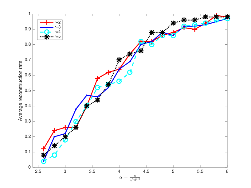
Figure 1: Average reconstruction rate of the proposed approach when $d=50$ and $r=2,3,4,5$. For each $r$ and $\alpha$, the algorithm is repeated for $50$ times.

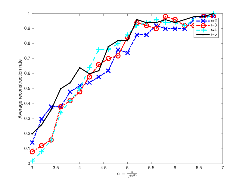
Figure 2: Average reconstruction rate of the proposed approach when $d=100$ and $r=2,3,4,5$. For each $r$ and $\alpha$, the algorithm is repeated for $50$ times.

As mentioned before, in addition to the gradient descent algorithm described in Section 5, several other algorithms can also be applied to optimize $F(\mathbf{X},\mathbf{Y},\mathbf{Z})$ locally. A notable example is the geometrical conjugate gradient descent algorithm on Riemannian manifolds proposed by Kressner et al. (2014). Although we have focused on the analysis of the gradient descent algorithm, we believe similar results could also be established for these other algorithms as well. In essence, the success of these methods is determined by the quality of the initialization, which the method from Section 4 could be readily applied. We leave the more rigorous theoretical analysis for future work, we conducted a set of numerical experiments to illustrate the similarity between these optimization algorithms while highlighting the crucial role of initialization.

We considered a similar setup as before with $d=50$,$r=5$ and $d=100,r=3$. We shall refer to our method as GoG and the geometrical conjugate gradient descent algorithm as GeoCG, for brevity. Note that the GeoCG algorithm was proposed without considering the theoretical requirement on the sample size and the algorithm is initiated with a random guess. We first tested both algorithms with a reliable initialization as proposed in Section 4. That is, we started with $\widehat{}\mathbf{U},\widehat{}\mathbf{V},\widehat{}\mathbf{W}$ obtained from the spectral algorithm and let $\widehat{\mathbf{C}}\in\mathbb{R}^{r\times r\times r}$ be the minimizer of (2). Then, the GeoCG(Spectral) algorithm is initialized from the starting point $\widehat{}\mathbf{A}^{(0)}=(\widehat{}\mathbf{U},\widehat{}\mathbf{V},\widehat{}\mathbf{W})\cdot\widehat{}\mathbf{C}$. For each $\alpha=\frac{n}{\sqrt{r}d^{3/2}}$, the GeoCG algorithm is repeated for $50$ times. The reconstruction rates are as shown in the Cyan curves in Figure 3 and 4. It is clear that both algorithms perform well and are comparable.

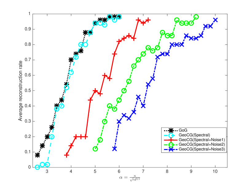
Figure 3: Comparison between GoG and GeoCG algorithm when $d=50$ and $r=5$. The successful rates of GeoCG algorithm depend on the initialization. Here GeoCG(Spectral) means that the GeoCG algorithm is initialized with the spectral methods as GoG algorithm. The black and Cyan curves show that GoG and GeoCG algorithm perform similarly when both are initialized with spectral methods. Here GeoCG(Spectral+Noise$X$) means that GeoCG algorithm is initialized with spectral methods plus random perturbation. If $X$ is larger, the perturbation is larger and the initialization is further away from the truth, in which case the reconstruction rate decreases.

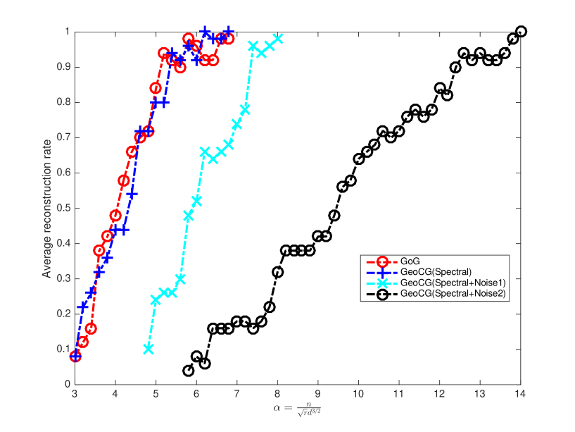
Figure 4: Comparison between GoG and GeoCG algorithm when $d=100$ and $r=3$. The successful rates of GeoCG algorithm depend on the initialization.

To illustrate that successful recovery hinges upon the appropriate initialization, we now consider applying GeoCG algorithm with a randomly perturbed spectral initialization. More specifically, the GeoCG algorithm is initialized with $\widehat{}\mathbf{A}^{(0)}+\sigma\mathbf{Z}$ where $\mathbf{Z}\in\mathbb{R}^{d\times d\times d}$ is a random tensor with i.i.d. standard normal entries and $\sigma>0$ represents the noise level. Figure 3 and 4 show that the reconstruction rate decreases when $\sigma$ gets larger.

These observations confirm the insights from our theoretical development: that the objective function $F$ is well-behaved locally and therefore with appropriate initialization can lead to successful recovery of low rank tensors.

7 Discussions

In this paper, we proved that with $n\geq C\mu_{0}^{3}r_{1}r_{2}r_{3}(rd_{1}d_{2}d_{3})^{1/2}\log^{7/2}(d)$ uniformly sampled entries, a tensor $\mathbf{T}$ of multilinear ranks ($r_{1},r_{2},r_{3}$) can be recovered with high probability with a polynomial time algorithm. In doing so, we argue that the underlying optimization problem is well behaved in a neighborhood around the truth and therefore, the sample size requirement is largely driven by our ability to initialize the algorithm appropriately. To this end, a new spectral method based on estimating the second moment of tensor unfoldings is proposed. In the low rank case, e.g., $r=O(1)$, this sample size requirement is essentially of the same order as $d^{3/2}$, up to a polynomial of $\log d$ term. This matches the sample size requirement for nuclear norm minimization which is NP hard to compute in general. An argument put forth by Barak and Moitra (2016) suggests that such a dependence on the dimension may be optimal for polynomial time algorithms unless a more efficient algorithm exists for the 3-SAT problem.

Even though our framework is established for third order tensors, it can be naturally extended to higher order tensors. Indeed, to complete a $k$th order tensor $\mathbf{T}\in\mathbb{R}^{d\times d\times\ldots\times d}$ with multilinear ranks $(r,r,\ldots,r)$, we can apply similar type of algorithms for optimizing over product of Grassmanianns. In order to ensure exact recovery, we can start with similar initialization where we unfold the tensor to $d\times d^{k-1}$ matrices. Following an identical argument, it can be derived in the same fashion that the sample size requirement for exact recovery now becomes

$$n\geq Cd^{k/2}{\rm polylog}(r,\log d)$$

for some constant $C>0$. Unlike the third order case, the dependence on the dimensionality ($d^{k/2}$) is worse than the nuclear norm minimization ($d^{3/2}$) for $k>3$. See Yuan and Zhang (2016b). In general, it remains unclear whether the requirement of $d^{k/2}$ is the best attainable for polynomial time algorithms for $k>3$.

8 Proofs

Throughout the proofs, we shall use $C$ and similarly $C_{1},C_{2}$ and etc. to denote generic numerical positive constants that may take different values at each appearance.

Proof of Theorem 1.

In view of Theorem 4, the proof of Theorem 1 is immediate if we are able to find an initial point $(\mathbf{X}^{(0)},\mathbf{Y}^{(0)},\mathbf{Z}^{(0)})\in\mathcal{N}\big{(}C(\alpha\kappa_{0}^{2}\log d)^{-1},3\mu_{0})$. Clearly, under the conditions on $n$ given in Theorem 1, the spectral initialization $(\widehat{}\mathbf{U},\widehat{}\mathbf{V},\widehat{}\mathbf{W})$ satisifies that

$$d_{\rm p}\Big{(}(\widehat{}\mathbf{U},\widehat{}\mathbf{V},\widehat{}\mathbf{W}),(\mathbf{U},\mathbf{V},\mathbf{W})\Big{)}\leq C(\alpha\kappa_{0}^{2}\log d)^{-1}$$

with probability at least $1-3d^{-\alpha}$. It remains to show that we can derive an incoherent initial value from $(\widehat{}\mathbf{U},\widehat{}\mathbf{V},\widehat{}\mathbf{W})$ in polynomial time, which is an immediate consequence of the following lemma due to Keshavan et al. (2009).

Lemma 2.

Let $\widehat{}\mathbf{U},\mathbf{U}\in\mathbb{R}^{d\times r}$ with $\widehat{}\mathbf{U}^{\top}\widehat{}\mathbf{U}=\mathbf{U}^{\top}\mathbf{U}=\mathbf{I}_{r}$ and $\mu(\mathbf{U})\leq\mu_{0}$. If $d_{\rm p}(\widehat{}\mathbf{U},\mathbf{U})\leq\delta\leq\frac{1}{16}$, then there exists an algorithm on $\widehat{}\mathbf{U}$ whose complexity is $O(dr^{2})$ which produces a candidate $\tilde{}\mathbf{U}\in\mathcal{G}(d,r)$ such that $\mu(\tilde{}\mathbf{U})\leq 3\mu_{0}$ and $d_{\rm p}(\tilde{}\mathbf{U},\mathbf{U})\leq 4\delta.$

By applying the algorithm claimed in Lemma 2 onto $\widehat{}\mathbf{U},\widehat{}\mathbf{V},\widehat{}\mathbf{W}$, we obtain $(\mathbf{X}^{(0)},\mathbf{Y}^{(0)},\mathbf{Z}^{(0)})=(\tilde{}\mathbf{U},\tilde{}\mathbf{V},\tilde{}\mathbf{W})\in\mathcal{N}\big{(}C(\alpha\kappa_{0}^{2}\log d)^{-1},3\mu_{0})$, which concludes the proof of Theorem 1. ∎

Proof of Theorem 2.

Note that $\widehat{\mathbf{N}}$ is actually U-statistics. Using a standard decoupling technique for U-statistics (see, e.g., de la Peña and Montgomery-Smith, 1995; De la Pena and Giné, 1999), we get

$$\mathbb{P}(\|\widehat{\mathbf{N}}-\mathbf{N}\|>t)\leq 15\mathbb{P}(15\|\tilde{\mathbf{N}}-\mathbf{N}\|>t)$$

for any $t>0$, where

$$\tilde{\mathbf{N}}:={1\over 2n(n-1)}\sum_{i\neq j}(\mathbf{X}_{i}\mathbf{Y}_{j}^{\top}+\mathbf{Y}_{j}\mathbf{X}_{i}^{\top}),$$

and $\{\mathbf{Y}_{i}:1\leq i\leq n\}$ is an independent copy of $\{\mathbf{X}_{i}:1\leq i\leq n\}$. We shall then focus, in what follows, on bounding $\mathbb{P}(\|\tilde{\mathbf{N}}-\mathbf{N}\|>t)$.

Observe that

$$\tilde{\mathbf{N}}={1\over 2n(n-1)}(\mathbf{S}_{1n}\mathbf{S}_{2n}^{\top}+\mathbf{S}_{2n}\mathbf{S}_{1n}^{\top})-{1\over 2n(n-1)}\sum_{i=1}^{n}(\mathbf{X}_{i}\mathbf{Y}_{i}^{\top}+\mathbf{Y}_{i}\mathbf{X}_{i}^{\top}),$$

where

$$\mathbf{S}_{1k}=\sum_{i=1}^{k}\mathbf{X}_{i},\qquad{\rm and}\qquad\mathbf{S}_{2k}=\sum_{i=1}^{k}\mathbf{Y}_{i}.$$

An application of Chernoff bound yields that, with probability at least $1-m^{-\alpha}$,

$$\|\mathbf{S}_{1n}\|_{\ell_{\infty}}\leq(3\alpha+7)m_{1}m_{2}\|\mathbf{M}\|_{\max}\left({n\over m_{2}}+\log m\right)$$

for any $\alpha>0$, where

$$\|\mathbf{S}_{1n}\|_{\ell_{\infty}}:=\max_{1\leq j\leq m_{2}}\sum_{1\leq i\leq m_{1}}\left|(\mathbf{S}_{1n})_{ij}\right|.$$

See, e.g., Yuan and Zhang (2016b). Denote this event by ${\cal E}_{1}$. On the other hand, as shown by Recht (2011), with probability at least $1-2m^{-\alpha}$,

$$\left\|{1\over n}\mathbf{S}_{1n}-\mathbf{M}\right\|\leq\sqrt{8(\alpha+1)m_{1}m_{2}m\log m\over 3n}\|\mathbf{M}\|_{\max},$$

and

$$\left\|{1\over n}\mathbf{S}_{2n}-\mathbf{M}\right\|\leq\sqrt{8(\alpha+1)m_{1}m_{2}m\log m\over 3n}\|\mathbf{M}\|_{\max}.$$

Denote this event by ${\cal E}_{2}$. Write ${\cal E}={\cal E}_{1}\cap{\cal E}_{2}$. It is not hard to see that for any $t\geq 0$,

$$\mathbb{P}\left\{\left\|\tilde{\mathbf{N}}-\mathbf{N}\right\|>t\right\}\leq\mathbb{P}\left\{\left\|\tilde{\mathbf{N}}-\mathbf{N}\right\|>t\bigcap{\cal E}\right\}+3m^{-\alpha}$$

We shall now proceed to bound the first probability on the right hand side.

Write

$$\tilde{\mathbf{N}}-\mathbf{N} = {1\over 2n(n-1)}\left[\left(\mathbf{S}_{1n}-n\mathbf{M}\right)(\mathbf{S}_{2n}-n\mathbf{M})^{\top}+(\mathbf{S}_{2n}-n\mathbf{M})\left(\mathbf{S}_{1n}-n\mathbf{M}\right)^{\top}\right]$$

$$\hskip 50.0pt+{1\over 2(n-1)}\left[\mathbf{M}\left(\mathbf{S}_{2n}-n\mathbf{M}\right)^{\top}+\left(\mathbf{S}_{2n}-n\mathbf{M}\right)\mathbf{M}^{\top}\right]$$

$$\hskip 50.0pt+{1\over 2(n-1)}\left[\mathbf{M}\left(\mathbf{S}_{1n}-n\mathbf{M}\right)^{\top}+\left(\mathbf{S}_{1n}-n\mathbf{M}\right)\mathbf{M}^{\top}\right]$$

$$\hskip 50.0pt-{1\over 2n(n-1)}\sum_{i=1}^{n}(\mathbf{X}_{i}\mathbf{Y}_{i}^{\top}+\mathbf{Y}_{i}\mathbf{X}_{i}^{\top}-2\mathbf{M}\mathbf{M}^{\top})$$

$$=: \mathbf{A}_{1}+\mathbf{A}_{2}+\mathbf{A}_{3}+\mathbf{A}_{4}.$$

We bound each of the four terms on the rightmost hand side separately. For brevity, write

$$\Delta_{1k}=\mathbf{S}_{1k}-k\mathbf{M},\qquad{\rm and}\qquad\Delta_{2k}=\mathbf{S}_{2k}-k\mathbf{M}.$$

We begin with

$$\mathbf{A}_{1}={1\over 2n(n-1)}\left(\Delta_{1n}\Delta_{2n}^{\top}+\Delta_{2n}\Delta_{1n}^{\top}\right).$$

By Markov inequality, for any $\lambda>0$,

$$\mathbb{P}\left\{\left\|\mathbf{A}_{1}\right\|>t\bigcap{\cal E}\right\}\leq\mathbb{P}\left\{\operatorname{tr}\exp\left(\lambda\mathbf{A}_{1}\right)>\exp(\lambda t)\bigcap{\cal E}\right\}\leq e^{-\lambda t}\mathbb{E}\operatorname{tr}\exp\left[\lambda\mathbf{A}_{1}{\bf 1}_{\cal E}\right].$$

Repeated use of Golden-Thompson inequality yields,

$$\mathbb{E}\operatorname{tr}\exp\left[\lambda\mathbf{A}_{1}{\bf 1}_{\cal E}\right] = \mathbb{E}\left(\mathbb{E}\left\{\operatorname{tr}\exp\left[\lambda\mathbf{A}_{1}\right]{\bf 1}_{\cal E}\biggr{|}\mathbf{S}_{1n}\right\}\right)$$

$$\leq \mathbb{E}\biggr{(}\mathbb{E}\left\{\operatorname{tr}\exp\left[{\lambda\over 2n(n-1)}(\Delta_{1n}\Delta_{2,n-1}^{\top}+\Delta_{2,n-1}\Delta_{1n}^{\top})\right]{\bf 1}_{\cal E}\biggr{|}\mathbf{S}_{1n}\right\}\times$$

$$\hskip 20.0pt\left\|\mathbb{E}\left\{\exp\left[{\lambda\over 2n(n-1)}(\Delta_{1n}(\mathbf{Y}_{n}-\mathbf{M})^{\top}+(\mathbf{Y}_{n}-\mathbf{M})\Delta_{1n}^{\top})\right]{\bf 1}_{\cal E}\biggr{|}\mathbf{S}_{1n}\right\}\right\|\biggl{)}$$

$$\leq \cdots\cdots$$

$$\leq \mathbb{E}\left(\left\|\mathbb{E}\left\{\exp\left[{\lambda\over 2n(n-1)}(\Delta_{1n}(\mathbf{Y}_{n}-\mathbf{M})^{\top}+(\mathbf{Y}_{n}-\mathbf{M})\Delta_{1n}^{\top})\right]{\bf 1}_{\cal E}\biggr{|}\mathbf{S}_{1n}\right\}\right\|^{n}\right)$$

By triangular inequality,

$$\left\|{\lambda\over 2n(n-1)}\left[\Delta_{1n}(\mathbf{Y}_{n}-\mathbf{M})^{\top}+(\mathbf{Y}_{n}-\mathbf{M})\Delta_{1n}^{\top}\right]\right\|\leq{\lambda\over n(n-1)}\left(\|\Delta_{1n}\mathbf{Y}_{n}^{\top}\|+\|\Delta_{1n}\mathbf{M}^{\top}\|\right).$$

Under the even ${\cal E}_{1}$,

$$\|\Delta_{1n}\mathbf{Y}_{n}^{\top}\| \leq \|\mathbf{S}_{1n}\mathbf{Y}_{n}^{\top}\|+n\|\mathbf{M}\mathbf{Y}_{n}^{\top}\|$$

$$\leq (3\alpha+7)m_{1}^{2}m_{2}^{2}\|\mathbf{M}\|^{2}_{\max}\left({n\over m_{2}}+\log m\right)+nm_{1}m_{2}\|\mathbf{M}\|_{\max}\|\mathbf{M}\|.$$

On the other hand, under the event ${\cal E}_{2}$,

$$\|\Delta_{1n}\mathbf{M}^{\top}\|\leq\|\Delta_{1n}\|\|\mathbf{M}\|\leq\sqrt{{8\over 3}n(\alpha+1)m_{1}m_{2}m\log m}\|\mathbf{M}\|_{\max}\|\mathbf{M}\|$$

Recall that

$$n\cdot\min\{m_{1},m_{2}\}\geq{8\over 3}(\alpha+1)\log m.$$

Then

$$\left\|{\lambda\over 2n(n-1)}\left[\Delta_{1n}(\mathbf{Y}_{n}-\mathbf{M})^{\top}+(\mathbf{Y}_{n}-\mathbf{M})\Delta_{1n}^{\top}\right]\right\|$$

$$\leq {\lambda\over n(n-1)}\left((3\alpha+7)m_{1}^{2}m_{2}^{2}\|\mathbf{M}\|^{2}_{\max}\left({n\over m_{2}}+\log m\right)+nm_{1}m_{2}\|\mathbf{M}\|_{\max}\|\mathbf{M}\|\right).$$

Therefore, for any

$$\lambda\leq n(n-1)\left((3\alpha+7)m_{1}^{2}m_{2}^{2}\|\mathbf{M}\|^{2}_{\max}\left({n\over m_{2}}+\log m\right)+nm_{1}m_{2}\|\mathbf{M}\|_{\max}\|\mathbf{M}\|\right)^{-1},$$

we get

$$\mathbb{E}\left\{\exp\left[{\lambda\over 2n(n-1)}\left[\Delta_{1n}(\mathbf{Y}_{n}-\mathbf{M})^{\top}+(\mathbf{Y}_{n}-\mathbf{M})\Delta_{1n}^{\top}\right]\right]{\bf 1}_{\cal E}\biggr{|}\mathbf{S}_{1n}\right\}$$

$$\preceq \mathbf{I}_{m_{1}}+\mathbb{E}\left\{\left[{\lambda\over 2n(n-1)}\left[\Delta_{1n}(\mathbf{Y}_{n}-\mathbf{M})^{\top}+(\mathbf{Y}_{n}-\mathbf{M})\Delta_{1n}^{\top}\right]\right]^{2}{\bf 1}_{\cal E}\biggr{|}\mathbf{S}_{1n}\right\}$$

$$\preceq \mathbf{I}_{m_{1}}+\mathbb{E}\left\{\left[{\lambda\over 2n(n-1)}\left(\Delta_{1n}\mathbf{Y}_{n}^{\top}+\mathbf{Y}_{n}\Delta_{1n}^{\top}\right)\right]^{2}{\bf 1}_{\cal E}\biggr{|}\mathbf{S}_{1n}\right\}$$

$$\preceq \mathbf{I}_{m_{1}}+{\lambda^{2}m_{1}m_{2}\|\mathbf{M}\|_{\max}^{2}\over 4n^{2}(n-1)^{2}}\left[(m_{1}+2)\Delta_{1n}\Delta_{1n}^{\top}+\operatorname{tr}(\Delta_{1n}\Delta_{1n}^{\top})\mathbf{I}_{m_{1}}\right]{\bf 1}_{\cal E}$$

where in the first inequality, we used the facts that

$$\exp(\mathbf{A})\leq\mathbf{I}_{d}+\mathbf{A}+\mathbf{A}^{2}$$

for any $\mathbf{A}\in\mathbb{R}^{d\times d}$ such that $\|\mathbf{A}\|\leq 1$, and

$$\mathbb{E}\left\{\left[{\lambda\over 2n(n-1)}\left[\Delta_{1n}(\mathbf{Y}_{n}-\mathbf{M})^{\top}+(\mathbf{Y}_{n}-\mathbf{M})\Delta_{1n}^{\top}\right]\right]{\bf 1}_{\cal E}\biggr{|}\mathbf{S}_{1n}\right\}=0.$$

Recall that

$$\operatorname{tr}(\Delta_{1n}\Delta_{1n}^{\top})\leq m_{1}\|\Delta_{1n}\Delta_{1n}^{\top}\|.$$

This implies that

$$\left\|\mathbb{E}\left\{\exp\left[{\lambda\over 2n(n-1)}\left[\Delta_{1n}(\mathbf{Y}_{n}-\mathbf{M})^{\top}+(\mathbf{Y}_{n}-\mathbf{M})\Delta_{1n}^{\top}\right]\right]{\bf 1}_{\cal E}\biggr{|}\mathbf{S}_{1n}\right\}\right\|$$

$$\leq 1+{\lambda^{2}\|\mathbf{M}\|_{\max}^{2}m_{1}^{2}m_{2}\over 2n^{2}(n-1)^{2}}\|\Delta_{1n}\Delta_{1n}^{\top}\|{\bf 1}_{\cal E}$$

$$\leq 1+{8(\alpha+1)\lambda^{2}\|\mathbf{M}\|_{\max}^{4}m_{1}^{3}m_{2}^{2}m\log m\over 3n(n-1)^{2}},$$

where the last inequality follows from the definition of ${\cal E}_{2}$. Thus,

$$\mathbb{E}\operatorname{tr}\exp\left[\lambda\mathbf{A}_{1}{\bf 1}_{\cal E}\right] \leq \exp\left[\lambda^{2}{16(\alpha+1)\|\mathbf{M}\|_{\max}^{4}m_{1}^{3}m_{2}^{2}m\log m\over 3(n-1)^{2}}\right].$$

Taking

$$\lambda = \min\biggl{\{}{3(n-1)^{2}t\over 64(\alpha+1)\|\mathbf{M}\|_{\max}^{4}m_{1}^{3}m_{2}^{2}m\log m},$$

$$\hskip 20.0pt{n(n-1)\over(6\alpha+14)m_{1}^{2}m_{2}^{2}\|\mathbf{M}\|^{2}_{\max}\left({n/m_{2}}+\log m\right)},{n(n-1)\over 2nm_{1}m_{2}\|\mathbf{M}\|_{\max}\|\mathbf{M}\|}\biggr{\}}$$

yields

$$\mathbb{P}\left\{\left\|\mathbf{A}_{1}\right\|>t\bigcap{\cal E}\right\} \leq \exp\biggl{(}-\min\biggl{\{}{3(n-1)^{2}t^{2}\over 128(\alpha+1)\|\mathbf{M}\|_{\max}^{4}m_{1}^{3}m_{2}^{2}m\log m},$$

$$\hskip 20.0pt{n(n-1)t\over(12\alpha+28)m_{1}^{2}m_{2}^{2}\|\mathbf{M}\|^{2}_{\max}\left({n/m_{2}}+\log m\right)},{n(n-1)t\over 4nm_{1}m_{2}\|\mathbf{M}\|_{\max}\|\mathbf{M}\|}\biggr{\}}\biggr{)}$$

We now proceed to bound $\mathbf{A}_{2}$ and $\mathbf{A}_{3}$. Both terms can be treated in an identical fashion and we shall consider only $\mathbf{A}_{2}$ here to fix ideas. As before, it can be derived that

$$\mathbb{P}\left\{\left\|\mathbf{A}_{2}\right\|>t\bigcap{\cal E}\right\}\leq\exp(-\lambda t)\left\|\mathbb{E}\left\{\exp\left[{\lambda\over 2(n-1)}(\mathbf{M}(\mathbf{Y}_{n}-\mathbf{M})^{\top}+(\mathbf{Y}_{n}-\mathbf{M})\mathbf{M}^{\top})\right]{\bf 1}_{\cal E}\right\}\right\|^{n}.$$

By taking

$$\lambda\leq{n-1\over\|\mathbf{M}\|^{2}+m_{1}m_{2}\|\mathbf{M}\|\|\mathbf{M}\|_{\max}},$$

we can ensure

$$\left\|{\lambda\over 2(n-1)}(\mathbf{M}(\mathbf{Y}_{n}-\mathbf{M})^{\top}+(\mathbf{Y}_{n}-\mathbf{M})\mathbf{M}^{\top})\right\| \leq {\lambda\over n-1}\left(\|\mathbf{M}\|^{2}+m_{1}m_{2}\|\mathbf{M}\|\|\mathbf{M}\|_{\max}\right)\leq 1.$$

If this is the case, we can derive as before that

$$\left\|\mathbb{E}\left\{\exp\left[{\lambda\over 2(n-1)}(\mathbf{M}(\mathbf{Y}_{n}-\mathbf{M})^{\top}+(\mathbf{Y}_{n}-\mathbf{M})\mathbf{M}^{\top})\right]{\bf 1}_{\cal E}\right\}\right\|$$

$$\leq 1+\left\|\mathbb{E}\left\{\left[{\lambda\over 2(n-1)}(\mathbf{M}(\mathbf{Y}_{n}-\mathbf{M})^{\top}+(\mathbf{Y}_{n}-\mathbf{M})\mathbf{M}^{\top})\right]^{2}{\bf 1}_{\cal E}\right\}\right\|$$

$$\leq 1+\left\|\mathbb{E}\left\{\left[{\lambda\over 2(n-1)}(\mathbf{M}\mathbf{Y}_{n}^{\top}+\mathbf{Y}_{n}\mathbf{M}^{\top})\right]^{2}{\bf 1}_{\cal E}\right\}\right\|$$

$$\leq 1+{\lambda^{2}m_{1}^{2}m_{2}\|\mathbf{M}\|_{\max}^{2}\|\mathbf{M}\|^{2}\over 2(n-1)^{2}}.$$

In particular, taking

$$\lambda=\min\left\{{n-1\over 2\|\mathbf{M}\|^{2}},{n-1\over 2m_{1}m_{2}\|\mathbf{M}\|\|\mathbf{M}\|_{\max}},{(n-1)^{2}t\over nm_{1}^{2}m_{2}\|\mathbf{M}\|_{\max}^{2}\|\mathbf{M}\|^{2}}\right\}$$

yields

$$\mathbb{P}\left\{\left\|\mathbf{A}_{2}\right\|>t\bigcap{\cal E}\right\}\leq\exp\left(-\min\left\{{(n-1)t\over 4\|\mathbf{M}\|^{2}},{(n-1)t\over 2m_{1}m_{2}\|\mathbf{M}\|\|\mathbf{M}\|_{\max}},{(n-1)^{2}t^{2}\over 2nm_{1}^{2}m_{2}\|\mathbf{M}\|_{\max}^{2}\|\mathbf{M}\|^{2}}\right\}\right).$$

Finally, we treat $\mathbf{A}_{4}$. Observe that

$$\|\mathbf{X}_{i}\mathbf{Y}_{i}^{\top}+\mathbf{Y}_{i}\mathbf{X}_{i}^{\top}-2\mathbf{M}\mathbf{M}^{\top}\| \leq 2\|\mathbf{X}_{i}\mathbf{Y}_{i}^{\top}\|+2\|\mathbf{M}\|^{2}$$

$$\leq 2m_{1}^{2}m_{2}^{2}\|\mathbf{M}\|_{\max}^{2}+2\|\mathbf{M}\|^{2}$$

$$\leq 4m_{1}^{2}m_{2}^{2}\|\mathbf{M}\|_{\max}^{2},$$

where the last inequality follows from the fact that $\|\mathbf{M}\|\leq\|\mathbf{M}\|_{\rm F}\leq\sqrt{m_{1}m_{2}}\|\mathbf{M}\|_{\max}$. On the other hand

$$\mathbb{E}\left(\mathbf{X}_{i}\mathbf{Y}_{i}^{\top}+\mathbf{Y}_{i}\mathbf{X}_{i}^{\top}-2\mathbf{M}\mathbf{M}^{\top}\right)^{2}\preceq\mathbb{E}\left(\mathbf{X}_{i}\mathbf{Y}_{i}^{\top}+\mathbf{Y}_{i}\mathbf{X}_{i}^{\top}\right)^{2}\preceq{2(m_{1}+1)m_{1}^{2}m_{2}^{3}\|\mathbf{M}\|_{\max}^{4}}\mathbf{I}.$$

An application of matrix Bernstein inequality (Tropp, 2012) yields

$$\mathbb{P}\left\{\|\mathbf{A}_{4}\|>t\cap{\cal E}\right\} \leq \mathbb{P}\left\{\|\mathbf{A}_{4}\|>t\right\}$$

$$\leq m_{1}\exp\left(-{n^{2}(n-1)^{2}t^{2}/2\over 2n(m_{1}+1)m_{1}^{2}m_{2}^{3}\|\mathbf{M}\|_{\max}^{4}+4m_{1}^{2}m_{2}^{2}\|\mathbf{M}\|_{\max}^{2}t/3}\right).$$

Putting the probability bounds for $\mathbf{A}_{1}$, $\mathbf{A}_{2}$, $\mathbf{A}_{3}$, $\mathbf{A}_{4}$ together, we have

$$\mathbb{P}\{\|\tilde{\mathbf{N}}-\mathbf{N}\|>t/15\}\leq\sum_{k=1}^{4}\mathbb{P}\{\|\mathbf{A}_{k}\|>t/60\cap{\cal E}\}+\mathbb{P}\{{\cal E}^{c}\}\leq 7m^{-\alpha}$$

by taking

$$t=C\cdot\alpha^{2}\cdot{m_{1}^{3/2}m_{2}^{3/2}\log m\over n}\left[\left(1+\frac{m_{1}}{m_{2}}\right)^{1/2}+{m_{1}^{1/2}m_{2}^{1/2}\over n}+\left({n\over m_{2}\log m}\right)^{1/2}\right]\cdot\|\mathbf{M}\|_{\max}^{2},$$

for some $C\geq 1680$. This immediately implies that

$$\mathbb{P}\big{\{}\|\widehat{}\mathbf{N}-\mathbf{N}\|\geq t\big{\}}\leq 105m^{-\alpha}.$$

The proof is then concluded by replacing $\alpha$ with $\alpha+\log_{m}105$ and adjusting the constant $C$ accordingly. ∎

Proof of Theorem 3.

Let $\mathbf{P}_{\mathbf{U}}$, $\mathbf{P}_{\mathbf{V}}$ and $\mathbf{P}_{\mathbf{W}}$ be the projection matrices onto the column space of $\mathbf{U}$, $\mathbf{V}$ and $\mathbf{W}$ respectively. Denote by $\mathbf{Q}_{\mathbf{T}}:\mathbb{R}^{d_{1}\times d_{2}\times d_{3}}\to\mathbb{R}^{d_{1}\times d_{2}\times d_{3}}$ a linear operator such that for any $\mathbf{A}\in\mathbb{R}^{d_{1}\times d_{2}\times d_{3}}$,

$$\mathbf{Q}_{\mathbf{T}}\mathbf{A}:=(\mathbf{P}_{\mathbf{U}},\mathbf{P}_{\mathbf{V}},\mathbf{P}_{\mathbf{W}})\cdot\mathbf{A}+(\mathbf{P}_{\mathbf{U}}^{\perp},\mathbf{P}_{\mathbf{V}},\mathbf{P}_{\mathbf{W}})\cdot\mathbf{A}+(\mathbf{P}_{\mathbf{U}},\mathbf{P}_{\mathbf{V}}^{\perp},\mathbf{P}_{\mathbf{W}})\cdot\mathbf{A}+(\mathbf{P}_{\mathbf{U}},\mathbf{P}_{\mathbf{V}},\mathbf{P}_{\mathbf{W}}^{\perp})\cdot\mathbf{A},$$

where $\mathbf{P}_{\mathbf{U}}^{\perp}=I-\mathbf{P}_{\mathbf{U}}$, and $\mathbf{P}_{\mathbf{V}}^{\perp}$ and $\mathbf{P}_{\mathbf{W}}^{\perp}$ are defined similarly. We shall also write $\mathbf{Q}_{\mathbf{T}}^{\perp}={\cal I}-\mathbf{Q}_{\mathbf{T}}$ where ${\cal I}$ is the identity map.

Basic facts about Grassmanianns.

Before proceeding, we shall first review some basic facts about the Grassmannians necessary for our proof. For further details, interested readers are referred to Edelman et al. (1998). To fix ideas, we shall focus on $\mathbf{U}\in\mathcal{G}(d_{1},r_{1})$. The tangent space of $\mathcal{G}(d_{1},r_{1})$ at $\mathbf{U}$, denoted by ${\cal T}_{\mathbf{U}}\subset\mathbb{R}^{d_{1}\times r_{1}}$, can be identified with the property $\mathbf{U}^{\top}\mathbf{D}_{\mathbf{U}}={\bf 0}$. The geodesic path from $\mathbf{U}$ to another point $\mathbf{X}\in{\cal G}(d_{1},r_{1})$ with respect to the canonical Riemann metric can be explicitly expressed as:

$$\mathbf{X}(t)=\mathbf{U}\mathbf{R}_{\mathbf{U}}\cos({\bf\Theta}_{\mathbf{U}}t)\mathbf{R}_{\mathbf{U}}^{\top}+\mathbf{L}_{\mathbf{U}}\sin({\bf\Theta_{\mathbf{U}}}t)\mathbf{R}_{\mathbf{U}}^{\top},\quad 0\leq t\leq 1$$

for some $\mathbf{D}_{\mathbf{U}}\in{\cal T}_{\mathbf{U}}$ and $\mathbf{D}_{\mathbf{U}}=\mathbf{L}_{\mathbf{U}}{\bf\Theta}_{\mathbf{U}}\mathbf{R}_{\mathbf{U}}^{\top}$ is its thin singular value decomposition. We can identify $\mathbf{X}(0)=\mathbf{U}$ and $\mathbf{X}(1)=\mathbf{X}$. The diagonal element of ${\bf\Theta}_{\mathbf{U}}$ lie in $[-\pi/2,\pi/2]$ and can be viewed as the principle angles between $\mathbf{U}$ and $\mathbf{X}$.

It is easy to check

$$d_{\rm p}(\mathbf{U},\mathbf{X})=\|\sin{\bf\Theta}_{\mathbf{U}}\|_{\rm F}\quad{\rm and}\quad\|{\bf\Delta}_{\mathbf{X}}\|_{\rm F}=\|\mathbf{U}-\mathbf{X}\|_{\rm F}=2\|\sin{\bf\Theta}_{\mathbf{U}}/2\|_{\rm F}.$$

Note that for any $\theta\in[0,\pi/2]$,

$$\frac{\theta}{2}\leq\sqrt{2}\sin(\theta/2)\leq\sin\theta\leq 2\sin(\theta/2)\leq\theta.$$

This implies that

$$d_{\rm p}(\mathbf{U},\mathbf{X})\leq\|\Delta_{\mathbf{X}}\|_{\rm F}\leq\sqrt{2}d_{\rm p}(\mathbf{U},\mathbf{X}).$$

Moreover,

$$\|\mathbf{U}^{\top}{\bf\Delta}_{\mathbf{X}}\|_{\rm F}=\|\cos({\bf\Theta}_{\mathbf{U}})-\mathbf{I}\|_{\rm F}=4\|\sin^{2}{\bf\Theta}_{\mathbf{U}}/2\|_{\rm F}\leq 2\|\sin{\bf\Theta}_{\mathbf{U}}\|_{\rm F}^{2}=2d_{\rm p}^{2}(\mathbf{U},\mathbf{X}).$$

With slight abuse of notation, write $\mathbf{D}_{\mathbf{X}}={d\mathbf{X}(t)\over dt}\big{|}_{t=1}\in{\cal T}_{\mathbf{X}}$. $\mathbf{D}_{\mathbf{X}}$ can be more explicitly expressed as

$$\mathbf{D}_{\mathbf{X}}=-\mathbf{U}\mathbf{R}_{\mathbf{U}}{\bf\Theta_{\mathbf{U}}}\sin{\bf\Theta_{\mathbf{U}}}\mathbf{R}_{\mathbf{U}}^{\top}+\mathbf{L}_{\mathbf{U}}{\bf\Theta}_{\mathbf{U}}\cos{\bf\Theta}_{\mathbf{U}}\mathbf{R}_{\mathbf{U}}^{\top}.$$

It is clear that

$$\|\mathbf{D}_{\mathbf{X}}\|_{\rm F}^{2}=\|{\bf\Theta}_{\mathbf{U}}\sin{\bf\Theta}_{\mathbf{U}}\|_{\rm F}^{2}+\|{\bf\Theta}_{\mathbf{U}}\cos{\bf\Theta}_{\mathbf{U}}\|_{\rm F}^{2}=\|{\bf\Theta}_{\mathbf{U}}\|_{\rm F}^{2},$$

so that

$$d_{\rm p}(\mathbf{U},\mathbf{X})\leq\|\mathbf{D}_{\mathbf{X}}\|_{\rm F}\leq 2d_{\rm p}(\mathbf{U},\mathbf{X}).$$

A couple of other useful relations can also be derived:

$$\|\mathbf{D}_{\mathbf{X}}-{\bf\Delta}_{\mathbf{X}}\|_{\rm F}^{2}=\|{\bf\Theta}_{\mathbf{U}}\|_{\rm F}^{2}+4\|\sin({\bf\Theta}_{\mathbf{U}}/2)\|_{\rm F}^{2}-2\langle{\bf\Theta}_{\mathbf{U}},\sin{\bf\Theta}_{\mathbf{U}}\rangle\leq\|{\bf\Theta_{\mathbf{U}}}-2\sin({\bf\Theta}_{\mathbf{U}}/2)\|_{\rm F}^{2}\leq d_{\rm p}^{4}(\mathbf{U},\mathbf{X}),$$

and

$$\|\mathbf{U}^{\top}\mathbf{D}_{\mathbf{X}}\|_{\rm F}=\|{\bf\Theta}_{\mathbf{U}}\sin{\bf\Theta}_{\mathbf{U}}\|_{\rm F}\leq 2\|\sin{\bf\Theta}_{\mathbf{U}}\|_{\rm F}^{2}=2d_{\rm p}^{2}(\mathbf{U},\mathbf{X}).$$

Lower bound of the first statement.

Note that

$$F(\mathbf{X},\mathbf{Y},\mathbf{Z})=\frac{1}{2}\big{\|}\mathcal{P}_{\Omega}\big{(}\widehat{\mathbf{T}}-\mathbf{T}\big{)}\big{\|}_{\rm F}^{2}\geq\frac{1}{4}\big{\|}\mathcal{P}_{\Omega}\mathbf{Q}_{\mathbf{T}}(\widehat{\mathbf{T}}-\mathbf{T})\big{\|}_{\rm F}^{2}-\frac{1}{2}\big{\|}\mathcal{P}_{\Omega}\mathbf{Q}_{\mathbf{T}}^{\perp}(\widehat{\mathbf{T}})\big{\|}_{\rm F}^{2},$$ (6)

where

$$\widehat{\mathbf{T}}=(\mathbf{X},\mathbf{Y},\mathbf{Z})\cdot\mathbf{C}$$

and $\mathbf{C}$ is given by (3). To derive the lower bound in the first statement, we shall lower bound $\|\mathcal{P}_{\Omega}\mathbf{Q}_{\mathbf{T}}(\widehat{\mathbf{T}}-\mathbf{T})\|_{\rm F}^{2}$ and upper bound $\|\mathcal{P}_{\Omega}\mathbf{Q}_{\mathbf{T}}^{\perp}(\widehat{\mathbf{T}})\|_{\rm F}^{2}$

By Lemma 5 of Yuan and Zhang (2016a), if $n\geq C_{1}\alpha\mu_{0}^{2}r^{2}d\log d$, then

$$\mathbb{P}\left\{\left\|\mathbf{Q}_{\mathbf{T}}\left(\mathcal{I}-\frac{d_{1}d_{2}d_{3}}{n}\mathcal{P}_{\Omega}\right)\mathbf{Q}_{\mathbf{T}}\right\|\geq\frac{1}{2}\right\}\leq d^{-\alpha},$$

where the operator norm is induced by the Frobenius norm, or the vectorized $\ell_{2}$ norm. Denote this event by ${\cal E}_{1}$. We shall now proceed under ${\cal E}_{1}$. On event ${\cal E}_{1}$,

$$\|\mathcal{P}_{\Omega}\mathbf{Q}_{\mathbf{T}}(\widehat{\mathbf{T}}-\mathbf{T})\|_{\rm F}^{2}\geq\left\langle\mathcal{P}_{\Omega}\mathbf{Q}_{\mathbf{T}}(\widehat{\mathbf{T}}-\mathbf{T}),\mathbf{Q}_{\mathbf{T}}(\widehat{}\mathbf{T}-\mathbf{T})\right\rangle\geq\frac{n}{2d_{1}d_{2}d_{3}}\|\mathbf{Q}_{\mathbf{T}}(\widehat{\mathbf{T}}-\mathbf{T})\|_{\rm F}^{2}.$$

Recall that

$$\mathbf{Q}_{\mathbf{T}}(\widehat{\mathbf{T}}-\mathbf{T})=(\mathbf{U},\mathbf{V},\mathbf{W})\cdot(\mathbf{G}-\mathbf{C})+({\bf\Delta}_{\mathbf{X}},\mathbf{V},\mathbf{W})\cdot\mathbf{C}+(\mathbf{U},{\bf\Delta}_{\mathbf{Y}},\mathbf{W})\cdot\mathbf{C}+(\mathbf{U},\mathbf{V},{\bf\Delta}_{\mathbf{Z}})\cdot\mathbf{C},$$ (7)

where

$${\bf\Delta_{X}}:=\mathbf{X}-\mathbf{U},\quad{\bf\Delta_{Y}}:=\mathbf{Y}-\mathbf{V},\quad{\rm and}\quad{\bf\Delta_{Z}}:=\mathbf{Z}-\mathbf{W}.$$

Therefore,

$$\|\mathbf{Q}_{\mathbf{T}}(\widehat{\mathbf{T}}-\mathbf{T})\|_{\rm F}^{2}= \|(\mathbf{U},\mathbf{V},\mathbf{W})\cdot(\mathbf{G}-\mathbf{C})\|_{\rm F}^{2}+\|({\bf\Delta}_{\mathbf{X}},\mathbf{V},\mathbf{W})\cdot\mathbf{C}\|_{\rm F}^{2}+\|(\mathbf{U},{\bf\Delta}_{\mathbf{Y}},\mathbf{W})\cdot\mathbf{C}\|_{\rm F}^{2}$$

$$+\|(\mathbf{U},\mathbf{V},{\bf\Delta}_{\mathbf{Z}})\cdot\mathbf{C}\|_{\rm F}^{2}+2\langle(\mathbf{U},\mathbf{V},\mathbf{W})\cdot(\mathbf{G}-\mathbf{C}),({\bf\Delta}_{\mathbf{X}},\mathbf{V},\mathbf{W})\cdot\mathbf{C}\rangle$$

$$+2\langle(\mathbf{U},\mathbf{V},\mathbf{W})\cdot(\mathbf{G}-\mathbf{C}),(\mathbf{U},{\bf\Delta}_{\mathbf{Y}},\mathbf{W})\cdot\mathbf{C}\rangle$$

$$+2\langle(\mathbf{U},\mathbf{V},\mathbf{W})\cdot(\mathbf{G}-\mathbf{C}),(\mathbf{U},\mathbf{V},{\bf\Delta}_{\mathbf{Z}})\cdot\mathbf{C}\rangle$$

$$+2\langle({\bf\Delta}_{\mathbf{X}},\mathbf{V},\mathbf{W})\cdot\mathbf{C},(\mathbf{U},{\bf\Delta}_{\mathbf{Y}},\mathbf{W})\cdot\mathbf{C}\rangle$$

$$+2\langle({\bf\Delta}_{\mathbf{X}},\mathbf{V},\mathbf{W})\cdot\mathbf{C},(\mathbf{U},\mathbf{V},{\bf\Delta}_{\mathbf{Z}})\cdot\mathbf{C}\rangle$$

$$+2\langle(\mathbf{U},{\bf\Delta}_{\mathbf{Y}},\mathbf{W})\cdot\mathbf{C},(\mathbf{U},\mathbf{V},{\bf\Delta}_{\mathbf{Z}})\cdot\mathbf{C}\rangle.$$

It is clear that

$$\|(\mathbf{U},\mathbf{V},\mathbf{W})\cdot(\mathbf{G}-\mathbf{C})\|_{\rm F}^{2}=\|\mathbf{G}-\mathbf{C}\|_{\rm F}^{2}.$$

We now bound each of the remaining terms on the righthand side separately.

Note that

$$\|({\bf\Delta}_{\mathbf{X}},\mathbf{V},\mathbf{W})\cdot\mathbf{C}\|_{\rm F}^{2} \geq \frac{1}{2}\|({\bf\Delta}_{\mathbf{X}},\mathbf{V},\mathbf{W})\cdot\mathbf{G}\|_{\rm F}^{2}-\|({\bf\Delta}_{\mathbf{X}},\mathbf{V},\mathbf{W})\cdot(\mathbf{C}-\mathbf{G})\|_{\rm F}^{2}$$

$$\geq {1\over 2}\sigma_{\min}^{2}({\cal M}_{1}(\mathbf{G}))\|{\bf\Delta}_{\mathbf{X}}\|_{\rm F}^{2}-\sigma_{\max}^{2}({\cal M}_{1}(\mathbf{C}-\mathbf{G}))\|{\bf\Delta}_{\mathbf{X}}\|_{\rm F}^{2}$$

$$\geq {1\over 2}\sigma_{\min}^{2}({\cal M}_{1}(\mathbf{G}))\|{\bf\Delta}_{\mathbf{X}}\|_{\rm F}^{2}-\|\mathbf{C}-\mathbf{G}\|_{\rm F}^{2}\|{\bf\Delta}_{\mathbf{X}}\|_{\rm F}^{2}$$

$$= {1\over 2}\sigma_{\min}^{2}({\cal M}_{1}(\mathbf{T}))\|{\bf\Delta}_{\mathbf{X}}\|_{\rm F}^{2}-\|\mathbf{C}-\mathbf{G}\|_{\rm F}^{2}\|{\bf\Delta}_{\mathbf{X}}\|_{\rm F}^{2}$$

Similarly,

$$\|(\mathbf{U},{\bf\Delta}_{\mathbf{Y}},\mathbf{W})\cdot\mathbf{C}\|_{\rm F}^{2}\geq{1\over 2}\sigma_{\min}^{2}({\cal M}_{2}(\mathbf{T}))\|{\bf\Delta}_{\mathbf{Y}}\|_{\rm F}^{2}-\|\mathbf{C}-\mathbf{G}\|_{\rm F}^{2}\|{\bf\Delta}_{\mathbf{Y}}\|_{\rm F}^{2},$$

and

$$\|(\mathbf{U},\mathbf{V},{\bf\Delta}_{\mathbf{Z}})\cdot\mathbf{C}\|_{\rm F}^{2}\geq{1\over 2}\sigma_{\min}^{2}({\cal M}_{3}(\mathbf{T}))\|{\bf\Delta}_{\mathbf{Z}}\|_{\rm F}^{2}-\|\mathbf{C}-\mathbf{G}\|_{\rm F}^{2}\|{\bf\Delta}_{\mathbf{Z}}\|_{\rm F}^{2}.$$

On the other hand,

$$\left|\langle(\mathbf{U},\mathbf{V},\mathbf{W})\cdot(\mathbf{G}-\mathbf{C}),({\bf\Delta}_{\mathbf{X}},\mathbf{V},\mathbf{W})\cdot\mathbf{C}\rangle\right|$$

$$= \left|\langle(\mathbf{U},\mathbf{V},\mathbf{W})\cdot(\mathbf{G}-\mathbf{C}),(\mathbf{P}_{\mathbf{U}}{\bf\Delta}_{\mathbf{X}},\mathbf{V},\mathbf{W})\cdot\mathbf{C}\rangle\right|$$

$$\leq \left\|(\mathbf{U},\mathbf{V},\mathbf{W})\cdot(\mathbf{G}-\mathbf{C})\right\|_{\rm F}\left\|(\mathbf{P}_{\mathbf{U}}{\bf\Delta}_{\mathbf{X}},\mathbf{V},\mathbf{W})\cdot\mathbf{C}\right\|_{\rm F}$$

$$\leq \|\mathbf{G}-\mathbf{C}\|_{\rm F}\|\mathbf{P}_{\mathbf{U}}{\bf\Delta}_{\mathbf{X}}\|_{\rm F}\|\mathbf{C}\|$$

$$\leq 2\|\mathbf{C}\|\|\mathbf{G}-\mathbf{C}\|_{\rm F}d_{\rm p}^{2}(\mathbf{U},\mathbf{X}).$$

Observe that

$$\|\mathbf{C}\|\leq\|\mathbf{G}\|+\|\mathbf{G}-\mathbf{C}\|\leq\|\mathbf{G}\|+\|\mathbf{G}-\mathbf{C}\|_{\rm F}=\|\mathbf{T}\|+\|\mathbf{G}-\mathbf{C}\|_{\rm F}.$$

We get

$$\left|\langle(\mathbf{U},\mathbf{V},\mathbf{W})\cdot(\mathbf{G}-\mathbf{C}),({\bf\Delta}_{\mathbf{X}},\mathbf{V},\mathbf{W})\cdot\mathbf{C}\rangle\right|\leq 2\|\mathbf{T}\|\|\mathbf{G}-\mathbf{C}\|_{\rm F}d_{\rm p}^{2}(\mathbf{U},\mathbf{X})$$

$$+2\|\mathbf{G}-\mathbf{C}\|_{\rm F}^{2}d_{\rm p}^{2}(\mathbf{U},\mathbf{X}).$$

Similarly,

$$\left|\langle(\mathbf{U},\mathbf{V},\mathbf{W})\cdot(\mathbf{G}-\mathbf{C}),(\mathbf{U},{\bf\Delta}_{\mathbf{Y}},\mathbf{W})\cdot\mathbf{C}\rangle\right|\leq 2\|\mathbf{T}\|\|\mathbf{G}-\mathbf{C}\|_{\rm F}d_{\rm p}^{2}(\mathbf{V},\mathbf{Y})$$

$$+2\|\mathbf{G}-\mathbf{C}\|_{\rm F}^{2}d_{\rm p}^{2}(\mathbf{V},\mathbf{Y}).$$

and

$$\left|\langle(\mathbf{U},\mathbf{V},\mathbf{W})\cdot(\mathbf{G}-\mathbf{C}),(\mathbf{U},\mathbf{V},{\bf\Delta}_{\mathbf{Z}})\cdot\mathbf{C}\rangle\right|\leq 2\|\mathbf{T}\|\|\mathbf{G}-\mathbf{C}\|_{\rm F}d_{\rm p}^{2}(\mathbf{W},\mathbf{Z})$$

$$+2\|\mathbf{G}-\mathbf{C}\|_{\rm F}^{2}d_{\rm p}^{2}(\mathbf{W},\mathbf{Z}).$$

Finally, we note that

$$\left|\langle({\bf\Delta}_{\mathbf{X}},\mathbf{V},\mathbf{W})\cdot\mathbf{C},(\mathbf{U},{\bf\Delta}_{\mathbf{Y}},\mathbf{W})\cdot\mathbf{C}\rangle\right|$$

$$= \left|\langle(\mathbf{P}_{\mathbf{U}}{\bf\Delta}_{\mathbf{X}},\mathbf{V},\mathbf{W})\cdot\mathbf{C},(\mathbf{U},\mathbf{P}_{\mathbf{V}}{\bf\Delta}_{\mathbf{Y}},\mathbf{W})\cdot\mathbf{C}\rangle\right|$$

$$\leq \|\mathbf{C}\|^{2}\|\mathbf{P}_{\mathbf{U}}{\bf\Delta}_{\mathbf{X}}\|_{\rm F}\|\mathbf{P}_{\mathbf{V}}{\bf\Delta}_{\mathbf{Y}}\|_{\rm F}$$

$$\leq 4\left(\|\mathbf{T}\|+\|\mathbf{G}-\mathbf{C}\|_{\rm F}\right)^{2}d_{\rm p}^{2}(\mathbf{U},\mathbf{X})d_{\rm p}^{2}(\mathbf{V},\mathbf{Y}).$$

And similarly,

$$\left|\langle({\bf\Delta}_{\mathbf{X}},\mathbf{V},\mathbf{W})\cdot\mathbf{C},(\mathbf{U},\mathbf{V},{\bf\Delta}_{\mathbf{Z}})\cdot\mathbf{C}\rangle\right|\leq 4\left(\|\mathbf{T}\|+\|\mathbf{G}-\mathbf{C}\|_{\rm F}\right)^{2}d_{\rm p}^{2}(\mathbf{U},\mathbf{X})d_{\rm p}^{2}(\mathbf{W},\mathbf{Z}),$$

and

$$\left|\langle(\mathbf{U},{\bf\Delta}_{\mathbf{Y}},\mathbf{W})\cdot\mathbf{C},(\mathbf{U},\mathbf{V},{\bf\Delta}_{\mathbf{Z}})\cdot\mathbf{C}\rangle\right|\leq 4\left(\|\mathbf{T}\|+\|\mathbf{G}-\mathbf{C}\|_{\rm F}\right)^{2}d_{\rm p}^{2}(\mathbf{V},\mathbf{Y})d_{\rm p}^{2}(\mathbf{W},\mathbf{Z}).$$

Putting all these bounds together, we get

$$\|\mathbf{Q}_{\mathbf{T}}(\widehat{\mathbf{T}}-\mathbf{T})\|_{\rm F}^{2}\geq\|\mathbf{G}-\mathbf{C}\|_{\rm F}^{2}+\left({\Lambda_{\min}^{2}\over 2}-\|\mathbf{C}-\mathbf{G}\|_{\rm F}^{2}\right)\left(\|{\bf\Delta_{X}}\|_{\rm F}^{2}+\|{\bf\Delta_{Y}}\|_{\rm F}^{2}+\|{\bf\Delta_{Z}}\|_{\rm F}^{2}\right)$$

$$-4\|\mathbf{T}\|\|\mathbf{G}-\mathbf{C}\|_{\rm F}d_{\rm p}^{2}((\mathbf{U},\mathbf{V},\mathbf{W}),(\mathbf{X},\mathbf{Y},\mathbf{Z}))$$

$$-4\|\mathbf{G}-\mathbf{C}\|_{\rm F}^{2}d_{\rm p}^{2}((\mathbf{U},\mathbf{V},\mathbf{W}),(\mathbf{X},\mathbf{Y},\mathbf{Z}))$$

$$-{8}\left(\|\mathbf{T}\|+\|\mathbf{G}-\mathbf{C}\|_{\rm F}\right)^{2}d_{\rm p}^{4}((\mathbf{U},\mathbf{V},\mathbf{W}),(\mathbf{X},\mathbf{Y},\mathbf{Z})),$$

where, with slight abuse of notation, we write

$$\Lambda_{\min}:=\min\left\{\sigma_{\min}({\cal M}_{1}(\mathbf{T})),\sigma_{\min}({\cal M}_{2}(\mathbf{T})),\sigma_{\min}({\cal M}_{3}(\mathbf{T}))\right\}.$$

Recall that

$$\|{\bf\Delta}_{\mathbf{X}}\|_{\rm F}\geq d_{\rm p}(\mathbf{X},\mathbf{U}),\quad\|{\bf\Delta}_{\mathbf{Y}}\|_{\rm F}\geq d_{\rm p}(\mathbf{Y},\mathbf{V}),\quad{\rm and}\quad\|{\bf\Delta}_{\mathbf{Z}}\|_{\rm F}\geq d_{\rm p}(\mathbf{Z},\mathbf{W}),$$

so that

$$\|{\bf\Delta_{X}}\|_{\rm F}^{2}+\|{\bf\Delta_{Y}}\|_{\rm F}^{2}+\|{\bf\Delta_{Z}}\|_{\rm F}^{2}\geq\frac{1}{3}d_{\rm p}^{2}((\mathbf{U},\mathbf{V},\mathbf{W}),(\mathbf{X},\mathbf{Y},\mathbf{Z})).$$

We can further bound $\|\mathbf{Q}_{\mathbf{T}}(\widehat{\mathbf{T}}-\mathbf{T})\|_{\rm F}^{2}$ by

$$\|\mathbf{Q}_{\mathbf{T}}(\widehat{\mathbf{T}}-\mathbf{T})\|_{\rm F}^{2} \geq \|\mathbf{G}-\mathbf{C}\|_{\rm F}^{2}$$

$$+\left({\Lambda_{\min}^{2}\over 6}-5\|\mathbf{C}-\mathbf{G}\|_{\rm F}^{2}-4\|\mathbf{T}\|\|\mathbf{G}-\mathbf{C}\|_{\rm F}\right)d_{\rm p}^{2}((\mathbf{U},\mathbf{V},\mathbf{W}),(\mathbf{X},\mathbf{Y},\mathbf{Z}))$$

$$-{16}\left(\|\mathbf{T}\|^{2}+\|\mathbf{G}-\mathbf{C}\|_{\rm F}^{2}\right)d_{\rm p}^{4}((\mathbf{U},\mathbf{V},\mathbf{W}),(\mathbf{X},\mathbf{Y},\mathbf{Z}))$$

Note that

$$\Lambda_{\min}\geq\kappa_{0}^{-1}\Lambda_{\max}(\mathbf{T})\geq\kappa_{0}^{-1}\|\mathbf{T}\|.$$

If $d_{\rm p}\big{(}(\mathbf{U},\mathbf{V},\mathbf{W}),(\mathbf{X},\mathbf{Y},\mathbf{Z})\big{)}\leq C(\alpha\kappa_{0}\log d)^{-1}$ for a sufficiently small $C$, we can ensure that

$$\|\mathbf{T}\|d_{\rm p}\big{(}(\mathbf{U},\mathbf{V},\mathbf{W}),(\mathbf{X},\mathbf{Y},\mathbf{Z})\big{)}\leq\frac{\Lambda_{\min}}{16}.$$

This implies that

$$\|\mathbf{Q}_{\mathbf{T}}(\widehat{\mathbf{T}}-\mathbf{T})\|_{\rm F}^{2}\geq\frac{5}{8}\|\mathbf{G}-\mathbf{C}\|_{\rm F}^{2}+\Big{(}\frac{\Lambda_{\min}^{2}}{12}-4\|\mathbf{T}\|\|\mathbf{G}-\mathbf{C}\|_{\rm F}\Big{)}d_{\rm p}^{2}\big{(}(\mathbf{U},\mathbf{V},\mathbf{W}),(\mathbf{X},\mathbf{Y},\mathbf{Z})\big{)}.$$

We have thus proved that under the event ${\cal E}_{1}$,

$$\|{\cal P}_{\Omega}\mathbf{Q}_{\mathbf{T}}(\widehat{}\mathbf{T}-\mathbf{T})\|_{\rm F}^{2} \geq \frac{5n}{16d_{1}d_{2}d_{3}}\|\mathbf{G}-\mathbf{C}\|_{\rm F}^{2}$$ (8)

$$+\frac{n}{2d_{1}d_{2}d_{3}}\Big{(}\frac{\Lambda_{\min}^{2}}{12}-4\|\mathbf{T}\|\|\mathbf{G}-\mathbf{C}\|_{\rm F}\Big{)}d_{\rm p}^{2}\big{(}(\mathbf{U},\mathbf{V},\mathbf{W}),(\mathbf{X},\mathbf{Y},\mathbf{Z})\big{)}.$$

Now consider upper bounding $\|\mathcal{P}_{\Omega}\mathbf{Q}_{\mathbf{T}}^{\perp}\widehat{\mathbf{T}}\|_{\rm F}^{2}$. By Chernoff bound, it is easy to see that with probability $1-d^{-\alpha}$,

$$\max_{\omega\in[d_{1}]\times[d_{2}]\times[d_{3}]}\sum_{i=1}^{n}\mathbb{I}(\omega_{i}=\omega)\leq C\alpha\log d$$

for some constant $C>0$. Denote this event by ${\cal E}_{2}$. Under this event

$$\|\mathcal{P}_{\Omega}\mathbf{Q}_{\mathbf{T}}^{\perp}\widehat{\mathbf{T}}\|_{\rm F}^{2}\leq C(\alpha\log d)\left\langle\mathcal{P}_{\Omega}\mathbf{Q}_{\mathbf{T}}^{\perp}\widehat{\mathbf{T}},\mathbf{Q}_{\mathbf{T}}^{\perp}\widehat{\mathbf{T}}\right\rangle.$$

To this end, it suffices to obtain upper bounds of

$$\left|\left\langle\mathcal{P}_{\Omega}\mathbf{Q}_{\mathbf{T}}^{\perp}\widehat{\mathbf{T}},\mathbf{Q}_{\mathbf{T}}^{\perp}\widehat{\mathbf{T}}\right\rangle\right|\leq\frac{n}{d_{1}d_{2}d_{3}}\|\mathbf{Q}_{\mathbf{T}}^{\perp}\widehat{}\mathbf{T}\|_{\rm F}^{2}+\left|\left\langle\mathcal{P}_{\Omega}\mathbf{Q}_{\mathbf{T}}^{\perp}\widehat{\mathbf{T}},\mathbf{Q}_{\mathbf{T}}^{\perp}\widehat{\mathbf{T}}\right\rangle-\frac{n}{d_{1}d_{2}d_{3}}\|\mathbf{Q}_{\mathbf{T}}^{\perp}\widehat{}\mathbf{T}\|_{\rm F}^{2}\right|.$$

For $\gamma_{1},\gamma_{2}>0$, define

$$\mathcal{K}(\gamma_{1},\gamma_{2}):=\big{\{}\mathbf{A}\in\mathbb{R}^{d_{1}\times d_{2}\times d_{3}}:\|\mathbf{A}\|_{\rm F}\leq 1,\|\mathbf{A}\|_{\max}\leq\gamma_{1},\|\mathbf{A}\|_{\star}\leq\gamma_{2}\big{\}}.$$

Consider the following empirical process:

$$\beta_{n}({\gamma_{1},\gamma_{2}}):=\underset{\mathbf{A}\in\mathcal{K}(\gamma_{1},\gamma_{2})}{\sup}\left|\frac{1}{n}\left\langle\mathcal{P}_{\Omega}\mathbf{A},\mathbf{A}\right\rangle-\frac{1}{d_{1}d_{2}d_{3}}\|\mathbf{A}\|_{\rm F}^{2}\right|.$$

Obviously,

$$\left|\left\langle\mathcal{P}_{\Omega}\mathbf{Q}_{\mathbf{T}}^{\perp}\widehat{\mathbf{T}},\mathbf{Q}_{\mathbf{T}}^{\perp}\widehat{\mathbf{T}}\right\rangle\right|\leq\frac{n}{d_{1}d_{2}d_{3}}\|\mathbf{Q}_{\mathbf{T}}^{\perp}\widehat{}\mathbf{T}\|_{\rm F}^{2}+n\|\mathbf{Q}_{\mathbf{T}}^{\perp}\widehat{}\mathbf{T}\|_{\rm F}^{2}\beta_{n}\Big{(}\frac{\|\mathbf{Q}_{\mathbf{T}}^{\perp}\widehat{}\mathbf{T}\|_{\max}}{\|\mathbf{Q}_{\mathbf{T}}^{\perp}\widehat{}\mathbf{T}\|_{\rm F}},\frac{\|\mathbf{Q}_{\mathbf{T}}^{\perp}\widehat{}\mathbf{T}\|_{\star}}{\|\mathbf{Q}_{\mathbf{T}}^{\perp}\widehat{}\mathbf{T}\|_{F}}\Big{)}.$$

We now appeal to the following lemma whose proof is given in Appendix C.

Lemma 3.

Given $0<\delta_{1}^{-}<\delta_{1}^{+}$, $0<\delta_{2}^{-}<\delta_{2}^{+}$ and $t\geq 1$, let

$$\bar{t}=t+\log\big{(}\log_{2}(\delta_{1}^{+}/\delta_{1}^{-})+\log_{2}(\delta_{2}^{+}/\delta_{2}^{-})+3\big{)}.$$

Then exists a universal constant $C>0$ such that with probability at least $1-e^{-t}$, the following bound holds for all $\gamma_{1}\in[\delta_{1}^{-},\delta_{1}^{+}]$ and all $\gamma_{2}\in[\delta_{2}^{-},\delta_{2}^{+}]$

$$\beta_{n}(\gamma_{1},\gamma_{2})\leq C\gamma_{1}\gamma_{2}\Big{(}\sqrt{\frac{d}{nd_{1}d_{2}d_{3}}}\log d+\frac{\log^{3/2}d}{n}\Big{)}+2\gamma_{1}\sqrt{\frac{\bar{t}}{nd_{1}d_{2}d_{3}}}+2\gamma_{1}^{2}\frac{\bar{t}}{n}$$

For any $\mathbf{A}\in\mathbb{R}^{d_{1}\times d_{2}\times d_{3}}$, we have $\frac{\|\mathbf{A}\|_{\max}}{\|\mathbf{A}\|_{\rm F}}\in[1/d_{1}d_{2}d_{3},1]$ and $\frac{\|\mathbf{A}\|_{\star}}{\|\mathbf{A}\|_{\rm F}}\in[1,d]$, we apply Lemma 3 with $\delta_{1}^{-}=\frac{1}{d_{1}d_{2}d_{3}}$, $\delta_{1}^{+}=1$, $\delta_{2}^{-}=1$ and $\delta_{2}^{+}=d$. By setting $t=\alpha\log d$ with ${\bar{t}}=t+\log\big{(}\log_{2}(d_{1})+\log_{2}(d_{2})+\log_{2}(d_{3})+\log_{2}(d)+3\big{)}\leq 6\alpha\log d$, we obtain that with probability at least $1-d^{-\alpha}$, for all $\gamma_{1}\in[(d_{1}d_{2}d_{3})^{-1},1]$ and $\gamma_{2}\in[1,d]$,

$$\beta_{n}(\gamma_{1},\gamma_{2})\leq C_{1}\alpha\gamma_{1}\gamma_{2}\Big{(}\sqrt{\frac{d}{nd_{1}d_{2}d_{3}}}\log d+\frac{\log^{3/2}d}{n}\Big{)}+C_{1}\alpha\gamma_{1}\sqrt{\frac{\log d}{nd_{1}d_{2}d_{3}}}+C_{1}\alpha\gamma_{1}^{2}\frac{\log d}{n}.$$

Denote this event by ${\cal E}_{3}$. Under ${\cal E}_{3}$, for any $\mathbf{A}\in\mathbb{R}^{d_{1}\times d_{2}\times d_{3}}$,

$$\|\mathbf{A}\|_{\rm F}^{2}\beta_{n}\Big{(}\frac{\|\mathbf{A}\|_{\max}}{\|\mathbf{A}\|_{\rm F}},\frac{\|\mathbf{A}\|_{\star}}{\|\mathbf{A}\|_{F}}\Big{)}\leq C_{1}\alpha\|\mathbf{A}\|_{\max}\|\mathbf{A}\|_{\star}\Big{(}\sqrt{\frac{d}{nd_{1}d_{2}d_{3}}}\log d+\frac{\log^{3/2}d}{n}\Big{)}$$

$$+C_{1}\alpha\|\mathbf{A}\|_{\max}\|\mathbf{A}\|_{\rm F}\sqrt{\frac{\log d}{nd_{1}d_{2}d_{3}}}+C_{1}\alpha\|\mathbf{A}\|_{\max}^{2}\frac{\log d}{n}.$$

This implies that

$$\left\langle\mathcal{P}_{\Omega}\mathbf{A},\mathbf{A}\right\rangle\leq\frac{n}{d_{1}d_{2}d_{3}}\|\mathbf{A}\|_{\rm F}^{2}+C\alpha\|\mathbf{A}\|_{\max}\|\mathbf{A}\|_{\star}\Big{(}\sqrt{\frac{nd}{d_{1}d_{2}d_{3}}}\log d+\log^{3/2}d\Big{)}.$$ (9)

We shall now focus on ${\cal E}_{3}$ and obtain

$$\left\langle\mathcal{P}_{\Omega}\mathbf{Q}_{\mathbf{T}}^{\perp}\widehat{}\mathbf{T},\mathbf{Q}_{\mathbf{T}}^{\perp}\widehat{}\mathbf{T}\right\rangle\leq \frac{n}{d_{1}d_{2}d_{3}}\|\mathbf{Q}_{\mathbf{T}}^{\perp}\widehat{}\mathbf{T}\|_{\rm F}^{2}$$

$$+C\alpha\|\mathbf{Q}_{\mathbf{T}}^{\perp}\widehat{}\mathbf{T}\|_{\max}\|\mathbf{Q}_{\mathbf{T}}^{\perp}\widehat{}\mathbf{T}\|_{\star}\Big{(}\sqrt{\frac{nd}{d_{1}d_{2}d_{3}}}\log d+\log^{3/2}d\Big{)}.$$ (10)

It remains to bound $\|\mathbf{Q}_{\mathbf{T}}^{\perp}\widehat{\mathbf{T}}\|_{\max}$, $\|\mathbf{Q}_{\mathbf{T}}^{\perp}\widehat{}\mathbf{T}\|_{\star}$ and $\|\mathbf{Q}_{\mathbf{T}}^{\perp}\widehat{\mathbf{T}}\|_{\rm F}$. Recall that

$$\mathbf{Q}_{\mathbf{T}}^{\perp}\widehat{}\mathbf{T}=(\mathbf{P}_{\mathbf{U}}^{\perp}\mathbf{X},\mathbf{P}_{\mathbf{V}}^{\perp}\mathbf{Y},\mathbf{Z})\cdot\mathbf{C}+(\mathbf{P}_{\mathbf{U}}^{\perp}\mathbf{X},\mathbf{Y},\mathbf{P}_{\mathbf{W}}^{\perp}\mathbf{Z})\cdot\mathbf{C}+(\mathbf{X},\mathbf{P}_{\mathbf{V}}^{\perp}\mathbf{Y},\mathbf{P}_{\mathbf{W}}^{\perp}\mathbf{Z})\cdot\mathbf{C}$$

$$+(\mathbf{P}_{\mathbf{U}}^{\perp}\mathbf{X},\mathbf{P}_{\mathbf{V}}^{\perp}\mathbf{Y},\mathbf{P}_{\mathbf{W}}^{\perp}\mathbf{Z})\cdot\mathbf{C}.$$

Recall that $\Lambda_{\max}(\mathbf{C}):=\max\{\|{\cal M}_{k}(\mathbf{C})\|,k=1,2,3\}$. Clearly, $\Lambda_{\max}(\mathbf{C})\leq\Lambda_{\max}+\|\mathbf{G}-\mathbf{C}\|_{\rm F}$ where, with slight abuse of notation, we write $\Lambda_{\max}:=\Lambda_{\max}(\mathbf{T})$ for brevity. Then,

$$\|\mathbf{Q}_{\mathbf{T}}^{\perp}\widehat{}\mathbf{T}\|_{\rm F}\leq\big{(}\Lambda_{\max}+\|\mathbf{G}-\mathbf{C}\|_{\rm F}\big{)}\Big{(}\|\mathbf{P}_{\mathbf{U}}^{\perp}\mathbf{X}\|_{\rm F}\|\mathbf{P}_{\mathbf{V}}^{\perp}\mathbf{Y}\|_{\rm F}+\|\mathbf{P}_{\mathbf{U}}^{\perp}\mathbf{X}\|_{\rm F}\|\mathbf{P}_{\mathbf{W}}^{\perp}\mathbf{Z}\|_{\rm F}+\|\mathbf{P}_{\mathbf{W}}^{\perp}\mathbf{Z}\|_{\rm F}\|\mathbf{P}_{\mathbf{V}}^{\perp}\mathbf{Y}\|_{\rm F}\Big{)}$$

$$+\big{(}\Lambda_{\max}+\|\mathbf{G}-\mathbf{C}\|_{\rm F}\big{)}\|\mathbf{P}_{\mathbf{U}}^{\perp}\mathbf{X}\|_{\rm F}\|\mathbf{P}_{\mathbf{V}}^{\perp}\mathbf{Y}\|_{\rm F}\|\mathbf{P}_{\mathbf{W}}^{\perp}\mathbf{Z}\|_{\rm F}.$$

Observe that

$$\|\mathbf{P}_{\mathbf{U}}^{\perp}\mathbf{X}\|_{\rm F}=\|\mathbf{P}_{\mathbf{U}}^{\perp}{\bf\Delta}_{\mathbf{X}}\|_{\rm F}\leq\|{\bf\Delta}_{\mathbf{X}}\|_{\rm F}\leq\sqrt{2}d_{\rm p}(\mathbf{U},\mathbf{X})$$

and

$$d_{\rm p}\big{(}(\mathbf{U},\mathbf{V},\mathbf{W}),(\mathbf{X},\mathbf{Y},\mathbf{Z})\big{)}\leq(C\alpha\kappa_{0}\log d)^{-1}.$$

Therefore,

$$\|\mathbf{Q}_{\mathbf{T}}^{\perp}\widehat{}\mathbf{T}\|_{\rm F} \leq \big{(}\Lambda_{\max}+\|\mathbf{G}-\mathbf{C}\|_{\rm F}\big{)}\Big{(}2d_{\rm p}^{2}\big{(}(\mathbf{U},\mathbf{V},\mathbf{W}),(\mathbf{X},\mathbf{Y},\mathbf{Z})\big{)}+2\sqrt{2}d_{\rm p}^{3}\big{(}(\mathbf{U},\mathbf{V},\mathbf{W}),(\mathbf{X},\mathbf{Y},\mathbf{Z})\big{)}\Big{)}$$

$$\leq 3\big{(}\Lambda_{\max}+\|\mathbf{G}-\mathbf{C}\|_{\rm F}\big{)}d_{\rm p}^{2}\big{(}(\mathbf{U},\mathbf{V},\mathbf{W}),(\mathbf{X},\mathbf{Y},\mathbf{Z})\big{)}.$$

It is clear that

$$\max_{k=1,2,3}\big{\{}\operatorname{rank}({\cal M}_{k}(\mathbf{Q}_{\mathbf{T}}^{\perp}\widehat{}\mathbf{T}))\big{\}}\leq 4r.$$

By Lemma 1,

$$\|\mathbf{Q}_{\mathbf{T}}^{\perp}\widehat{}\mathbf{T}\|_{\star}\leq 4r\|\mathbf{Q}_{\mathbf{T}}^{\perp}\widehat{}\mathbf{T}\|_{\rm F}\leq 12r\big{(}\Lambda_{\max}+\|\mathbf{G}-\mathbf{C}\|_{\rm F}\big{)}d_{\rm p}^{2}\big{(}(\mathbf{U},\mathbf{V},\mathbf{W}),(\mathbf{X},\mathbf{Y},\mathbf{Z})\big{)}.$$

Because of the incoherence condition

$$\max\{\mu({\bf\Delta}_{\mathbf{X}}),\mu({\bf\Delta}_{\mathbf{Y}}),\mu({\bf\Delta}_{\mathbf{Z}})\}\leq 9\mu_{0},$$

we get

$$\|\mathbf{Q}_{\mathbf{T}}^{\perp}\widehat{}\mathbf{T}\|_{\max}\leq 54\big{(}\Lambda_{\max}+\|\mathbf{C}-\mathbf{G}\|_{\rm F}\big{)}\mu_{0}^{3/2}\sqrt{\frac{r_{1}r_{2}r_{3}}{d_{1}d_{2}d_{3}}}.$$

By putting the bounds of $\|\mathbf{Q}_{\mathbf{T}}^{\perp}\widehat{}\mathbf{T}\|_{\rm F},\|\mathbf{Q}_{\mathbf{T}}^{\perp}\widehat{}\mathbf{T}\|_{\max}$ and $\|\mathbf{Q}_{\mathbf{T}}^{\perp}\widehat{}\mathbf{T}\|_{\star}$ into (10), we conclude that on event ${\cal E}_{3}$,

$$\Big{<}{\cal P}_{\Omega}\mathbf{Q}_{\mathbf{T}}^{\perp}\widehat{}\mathbf{T},\mathbf{Q}_{\mathbf{T}}^{\perp}\widehat{}\mathbf{T}\Big{>}\leq \frac{9n}{d_{1}d_{2}d_{3}}\big{(}\Lambda_{\max}+\|\mathbf{G}-\mathbf{C}\|_{\rm F}\big{)}^{2}d_{\rm p}^{4}\big{(}(\mathbf{U},\mathbf{V},\mathbf{W}),(\mathbf{X},\mathbf{Y},\mathbf{Z})\big{)}$$

$$+C_{1}\bigg{(}\alpha r(\Lambda_{\max}+\|\mathbf{G}-\mathbf{C}\|_{\rm F})^{2}\mu_{0}^{3/2}\sqrt{\frac{r_{1}r_{2}r_{3}}{d_{1}d_{2}d_{3}}}\Big{(}\sqrt{\frac{nd}{d_{1}d_{2}d_{3}}}\log d+\log^{3/2}d\Big{)}\bigg{)}$$

$$\times d_{\rm p}^{2}\big{(}(\mathbf{U},\mathbf{V},\mathbf{W}),(\mathbf{X},\mathbf{Y},\mathbf{Z})\big{)}$$ (11)

for a universal constant $C_{1}>0$. If $d_{\rm p}\big{(}(\mathbf{U},\mathbf{V},\mathbf{W}),(\mathbf{X},\mathbf{Y},\mathbf{Z})\big{)}\leq(C_{2}\alpha\kappa_{0}\log d)^{-1}$ and

$$n\geq C_{2}\Big{(}\alpha^{4}\mu_{0}^{3}\kappa_{0}^{4}r^{2}r_{1}r_{2}r_{3}d\log^{4}d+\alpha^{2}\mu_{0}^{3/2}\kappa_{0}^{2}r(r_{1}r_{2}r_{3}d_{1}d_{2}d_{3})^{1/2}\log^{5/2}d\Big{)}.$$

The above upper bound can be simplified as

$$\Big{<}{\cal P}_{\Omega}\mathbf{Q}_{\mathbf{T}}^{\perp}\widehat{}\mathbf{T},\mathbf{Q}_{\mathbf{T}}^{\perp}\widehat{}\mathbf{T}\Big{>} \leq \frac{n}{8C\alpha d_{1}d_{2}d_{3}\log d}\|\mathbf{G}-\mathbf{C}\|_{\rm F}^{2}$$ (12)

$$+\frac{n}{96C\alpha d_{1}d_{2}d_{3}\log d}\Lambda_{\min}^{2}d_{\rm p}^{2}\big{(}(\mathbf{U},\mathbf{V},\mathbf{W}),(\mathbf{X},\mathbf{Y},\mathbf{Z})\big{)}.$$

Therefore, under ${\cal E}_{2}\cap{\cal E}_{3}$,

$$\|\mathcal{P}_{\Omega}\mathbf{Q}_{\mathbf{T}}^{\perp}\widehat{\mathbf{T}}\|_{\rm F}^{2}\leq\frac{n}{8d_{1}d_{2}d_{3}}\|\mathbf{G}-\mathbf{C}\|_{\rm F}^{2}+\frac{n}{96d_{1}d_{2}d_{3}}\Lambda_{\min}^{2}d_{\rm p}^{2}((\mathbf{U},\mathbf{V},\mathbf{W}),(\mathbf{X},\mathbf{Y},\mathbf{Z})).$$ (13)

Combining (6),(8) and (13), we conclude that

$$F(\mathbf{X},\mathbf{Y},\mathbf{Z}) \geq \frac{n}{64d_{1}d_{2}d_{3}}\|\mathbf{G}-\mathbf{C}\|_{\rm F}^{2}$$ (14)

$$+\frac{n}{d_{1}d_{2}d_{3}}\Big{(}{\Lambda_{\min}^{2}\over 192}-\|\mathbf{T}\|\|\mathbf{G}-\mathbf{C}\|_{\rm F}\Big{)}d_{\rm p}^{2}((\mathbf{U},\mathbf{V},\mathbf{W}),(\mathbf{X},\mathbf{Y},\mathbf{Z})),$$

with probability at least

$$\mathbb{P}\{{\cal E}_{1}\cap{\cal E}_{2}\cap{\cal E}_{3}\}\geq 1-3d^{-\alpha}.$$

Upper bound of the first statement.

Let

$$\tilde{\mathbf{T}}=(\mathbf{X},\mathbf{Y},\mathbf{Z})\cdot\mathbf{G}.$$

By definition of $\widehat{\mathbf{T}}$,

$$F(\mathbf{X},\mathbf{Y},\mathbf{Z})={1\over 2}\|{\cal P}_{\Omega}(\widehat{\mathbf{T}}-\mathbf{T})\|_{\rm F}^{2}\leq{1\over 2}\|{\cal P}_{\Omega}(\tilde{\mathbf{T}}-\mathbf{T})\|_{\rm F}^{2}\leq\|{\cal P}_{\Omega}\mathbf{Q}_{\mathbf{T}}(\tilde{\mathbf{T}}-\mathbf{T})\|_{\rm F}^{2}+\|{\cal P}_{\Omega}\mathbf{Q}_{\mathbf{T}}^{\perp}\tilde{\mathbf{T}}\|_{\rm F}^{2}$$

Again, by Lemma 5 of Yuan and Zhang (2016a), on event ${\cal E}_{1}\cap{\cal E}_{2}$,

$$\|{\cal P}_{\Omega}\mathbf{Q}_{\mathbf{T}}(\tilde{\mathbf{T}}-\mathbf{T})\|_{\rm F}^{2} \leq C(\alpha\log d)\left\langle{\cal P}_{\Omega}\mathbf{Q}_{\mathbf{T}}(\tilde{}\mathbf{T}-\mathbf{T}),\mathbf{Q}_{\mathbf{T}}(\tilde{}\mathbf{T}-\mathbf{T})\right\rangle$$

$$\leq {3C\alpha n\log d\over 2d_{1}d_{2}d_{3}}\|\mathbf{Q}_{\mathbf{T}}(\tilde{\mathbf{T}}-\mathbf{T})\|_{\rm F}^{2}.$$

Recall that

$$\mathbf{Q}_{\mathbf{T}}(\tilde{\mathbf{T}}-\mathbf{T})=({\bf\Delta}_{\mathbf{X}},\mathbf{V},\mathbf{W})\cdot\mathbf{G}+(\mathbf{U},{\bf\Delta}_{\mathbf{Y}},\mathbf{W})\cdot\mathbf{G}+(\mathbf{U},\mathbf{V},{\bf\Delta}_{\mathbf{Z}})\cdot\mathbf{G}.$$

We have

$$\|\mathbf{Q}_{\mathbf{T}}(\tilde{\mathbf{T}}-\mathbf{T})\|_{\rm F}^{2} \leq 3\left(\|({\bf\Delta}_{\mathbf{X}},\mathbf{V},\mathbf{W})\cdot\mathbf{G}\|_{\rm F}^{2}+\|(\mathbf{U},{\bf\Delta}_{\mathbf{Y}},\mathbf{W})\cdot\mathbf{G}\|_{\rm F}^{2}+\|(\mathbf{U},\mathbf{V},{\bf\Delta}_{\mathbf{Z}})\cdot\mathbf{G}\|_{\rm F}^{2}\right).$$

Note that

$$\|({\bf\Delta}_{\mathbf{X}},\mathbf{V},\mathbf{W})\cdot\mathbf{G}\|_{\rm F}^{2}\leq\sigma_{\max}^{2}({\cal M}_{1}(\mathbf{G}))\|{\bf\Delta}_{\mathbf{X}}\|_{\rm F}^{2}\leq\Lambda_{\max}^{2}\|{\bf\Delta}_{\mathbf{X}}\|_{\rm F}^{2}.$$

Similar bounds hold for $\|(\mathbf{U},{\bf\Delta}_{\mathbf{Y}},\mathbf{W})\cdot\mathbf{G}\|_{\rm F}^{2}$ and $\|(\mathbf{U},\mathbf{V},{\bf\Delta}_{\mathbf{Z}})\cdot\mathbf{G}\|_{\rm F}^{2}$. We get on event ${\cal E}_{1}\cap{\cal E}_{2}$,

$$\|{\cal P}_{\Omega}\mathbf{Q}_{\mathbf{T}}(\tilde{\mathbf{T}}-\mathbf{T})\|_{\rm F}^{2}\leq{9C\alpha n\log d\over d_{1}d_{2}d_{3}}\Lambda_{\max}^{2}d^{2}_{\rm p}((\mathbf{U},\mathbf{V},\mathbf{W}),(\mathbf{X},\mathbf{Y},\mathbf{Z})).$$ (15)

On the other hand, following the same argument for bounding $\|{\cal P}_{\Omega}\mathbf{Q}_{\mathbf{T}}^{\perp}\widehat{\mathbf{T}}\|_{\rm F}^{2}$ as in (13), we can show that

$$\|{\cal P}_{\Omega}\mathbf{Q}_{\mathbf{T}}^{\perp}\tilde{\mathbf{T}}\|_{\rm F}^{2}\leq C\alpha\log d\Big{<}{\cal P}_{\Omega}\mathbf{Q}_{\mathbf{T}}^{\perp}\tilde{\mathbf{T}},\mathbf{Q}_{\mathbf{T}}^{\perp}\tilde{}\mathbf{T}\Big{>}\leq{n\over 96d_{1}d_{2}d_{3}}\Lambda_{\min}^{2}d^{2}_{\rm p}((\mathbf{U},\mathbf{V},\mathbf{W}),(\mathbf{X},\mathbf{Y},\mathbf{Z})),$$

under the event ${\cal E}_{1}\cap{\cal E}_{2}\cap{\cal E}_{3}$. In summary, we get on event ${\cal E}_{1}\cap{\cal E}_{2}\cap{\cal E}_{3}$,

$${d_{1}d_{2}d_{3}\over n}F(\mathbf{X},\mathbf{Y},\mathbf{Z})\leq 10C\alpha\Lambda_{\max}^{2}d^{2}_{\rm p}((\mathbf{U},\mathbf{V},\mathbf{W}),(\mathbf{X},\mathbf{Y},\mathbf{Z}))\log d.$$ (16)

The bounds (14) and (16) imply that

$$\frac{n}{64d_{1}d_{2}d_{3}}\|\mathbf{G}-\mathbf{C}\|_{\rm F}^{2}+\frac{n}{d_{1}d_{2}d_{3}}\Big{(}\frac{\Lambda_{\min}^{2}}{192}-\|\mathbf{T}\|\|\mathbf{G}-\mathbf{C}\|_{\rm F}\Big{)}d_{\rm p}^{2}\big{(}(\mathbf{U},\mathbf{V},\mathbf{W}),(\mathbf{X},\mathbf{Y},\mathbf{Z})\big{)}$$

$$\leq F(\mathbf{X},\mathbf{Y},\mathbf{Z})\leq\frac{10C\alpha n}{d_{1}d_{2}d_{3}}\Lambda_{\max}^{2}d_{\rm p}^{2}\big{(}(\mathbf{U},\mathbf{V},\mathbf{W}),(\mathbf{X},\mathbf{Y},\mathbf{Z})\big{)}\log d$$

which guarantees that

$$\|\mathbf{G}-\mathbf{C}\|_{\rm F}\leq C(\alpha\log d)^{1/2}\Lambda_{\max}d_{\rm p}\big{(}(\mathbf{U},\mathbf{V},\mathbf{W}),(\mathbf{X},\mathbf{Y},\mathbf{Z})\big{)}.$$ (17)

Recall that $\Lambda_{\max}\leq\bar{\Lambda}$ and $\Lambda_{\min}\geq\underline{\Lambda}$. We conclude that on event ${\cal E}_{1}\cap{\cal E}_{2}\cap{\cal E}_{3}$,

$$\frac{1}{128}\|\mathbf{G}-\mathbf{C}\|_{\rm F}^{2}+\frac{1}{384}\underline{\Lambda}^{2}d_{\rm p}^{2}\big{(}(\mathbf{U},\mathbf{V},\mathbf{W}),(\mathbf{X},\mathbf{Y},\mathbf{Z})\big{)}$$

$$\leq\frac{d_{1}d_{2}d_{3}}{n}F(\mathbf{X},\mathbf{Y},\mathbf{Z})\leq C(\alpha\log d)\bar{\Lambda}^{2}d_{\rm p}^{2}\big{(}(\mathbf{X},\mathbf{Y},\mathbf{Z}),(\mathbf{U},\mathbf{V},\mathbf{W})\big{)}.$$

Second statement.

Observe that

$$\|{\rm grad}\ F(\mathbf{X},\mathbf{Y},\mathbf{Z})\|_{\rm F}\geq\frac{\left\langle{\rm grad}\ F(\mathbf{X},\mathbf{Y},\mathbf{Z}),(\mathbf{D}_{\mathbf{X}},\mathbf{D}_{\mathbf{Y}},\mathbf{D}_{\mathbf{Z}})\right\rangle}{\left(\|\mathbf{D}_{\mathbf{X}}\|^{2}_{\rm F}+\|\mathbf{D}_{\mathbf{Y}}\|^{2}_{\rm F}+\|\mathbf{D}_{\mathbf{Z}}\|^{2}_{\rm F}\right)^{1/2}}.$$ (18)

Write

$$\mathbf{H}=(\mathbf{D}_{\mathbf{X}},\mathbf{Y},\mathbf{Z})\cdot\mathbf{C}+(\mathbf{X},\mathbf{D}_{\mathbf{Y}},\mathbf{Z})\cdot\mathbf{C}+(\mathbf{X},\mathbf{Y},\mathbf{D}_{\mathbf{Z}})\cdot\mathbf{C}.$$

Then

$$\left\langle{\rm grad}\ F(\mathbf{X},\mathbf{Y},\mathbf{Z}),(\mathbf{D}_{\mathbf{X}},\mathbf{D}_{\mathbf{Y}},\mathbf{D}_{\mathbf{Z}})\right\rangle=\left\langle{\cal P}_{\Omega}(\widehat{\mathbf{T}}-\mathbf{T}),\mathbf{H}\right\rangle.$$

Denote by

$$\mathbf{H}_{1}=(\mathbf{D}_{\mathbf{X}},\mathbf{V},\mathbf{W})\cdot\mathbf{C}+(\mathbf{U},\mathbf{D}_{\mathbf{Y}},\mathbf{W})\cdot\mathbf{C}+(\mathbf{U},\mathbf{V},\mathbf{D}_{\mathbf{Z}})\cdot\mathbf{C}$$

and

$$\mathbf{H}_{2}:= (\mathbf{D}_{\mathbf{X}},{\bf\Delta_{Y}},\mathbf{W})\cdot\mathbf{C}+(\mathbf{D}_{\mathbf{X}},\mathbf{V},{\bf\Delta_{Z}})\cdot\mathbf{C}+(\mathbf{D}_{\mathbf{X}},{\bf\Delta_{Y}},{\bf\Delta_{Z}})\cdot\mathbf{C}+({\bf\Delta_{X}},\mathbf{D}_{\mathbf{Y}},\mathbf{W})\cdot\mathbf{C}$$

$$+ (\mathbf{U},\mathbf{D}_{\mathbf{Y}},{\bf\Delta_{Z}})\cdot\mathbf{C}+({\bf\Delta_{X}},\mathbf{D}_{\mathbf{Y}},{\bf\Delta_{Z}})\cdot\mathbf{C}+({\bf\Delta_{X}},\mathbf{V},\mathbf{D}_{\mathbf{Z}})\cdot\mathbf{C}+(\mathbf{U},{\bf\Delta_{Y}},\mathbf{D}_{\mathbf{Z}})\cdot\mathbf{C}$$

$$+ ({\bf\Delta_{X}},{\bf\Delta_{Y}},\mathbf{D}_{\mathbf{Z}})\cdot\mathbf{C}.$$

Then, $\mathbf{H}=\mathbf{H}_{1}+\mathbf{H}_{2}$ and $\mathbf{Q}_{\mathbf{T}}\mathbf{H}_{1}=\mathbf{H}_{1}$. We write

$$\left\langle{\cal P}_{\Omega}(\widehat{\mathbf{T}}-\mathbf{T}),\mathbf{H}\right\rangle=\left\langle{\cal P}_{\Omega}\mathbf{Q}_{\mathbf{T}}(\widehat{\mathbf{T}}-\mathbf{T}),\mathbf{H}_{1}\right\rangle+\left\langle{\cal P}_{\Omega}\mathbf{Q}_{\mathbf{T}}^{\perp}\widehat{\mathbf{T}},\mathbf{H}_{1}\right\rangle+\left\langle{\cal P}_{\Omega}(\widehat{\mathbf{T}}-\mathbf{T}),\mathbf{H}_{2}\right\rangle.$$

Since $\mathbf{Q}_{\mathbf{T}}\mathbf{H}_{1}=\mathbf{H}_{1}$, we can show that under the event ${\cal E}_{1}$,

$$\left\langle{\cal P}_{\Omega}\mathbf{Q}_{\mathbf{T}}(\widehat{\mathbf{T}}-\mathbf{T}),\mathbf{H}_{1}\right\rangle\geq\frac{d_{1}d_{2}d_{3}}{2n}\left\langle\mathbf{Q}_{\mathbf{T}}(\widehat{}\mathbf{T}-\mathbf{T}),\mathbf{H}_{1}\right\rangle.$$

Based on the lower bound of $\left\langle\mathbf{Q}_{\mathbf{T}}(\widehat{}\mathbf{T}-\mathbf{T}),\mathbf{H}_{1}\right\rangle$ proved in Appendix D, we conclude that on event $\mathcal{E}_{1}\cap{\cal E}_{2}\cap{\cal E}_{3}$,

$$\left\langle{\cal P}_{\Omega}\mathbf{Q}_{\mathbf{T}}(\widehat{\mathbf{T}}-\mathbf{T}),\mathbf{H}_{1}\right\rangle\geq\frac{n}{8d_{1}d_{2}d_{3}}\zeta_{1}\geq\frac{\Lambda_{\min}^{2}}{128}\frac{n}{d_{1}d_{2}d_{3}}d_{\rm p}^{2}\big{(}(\mathbf{U},\mathbf{V},\mathbf{W}),(\mathbf{X},\mathbf{Y},\mathbf{Z})\big{)}$$ (19)

where $\zeta_{1}:=\|({\bf\Delta}_{\mathbf{X}},\mathbf{V},\mathbf{W})\cdot\mathbf{C}+(\mathbf{U},{\bf\Delta}_{\mathbf{Y}},\mathbf{W})\cdot\mathbf{C}+(\mathbf{U},\mathbf{V},{\bf\Delta}_{\mathbf{Z}})\cdot\mathbf{C}\|_{\rm F}^{2}$ with (see Appendix D)

$$\zeta_{1}\geq\frac{1}{16}\Lambda_{\min}^{2}d_{\rm p}^{2}\big{(}(\mathbf{U},\mathbf{V},\mathbf{W}),(\mathbf{X},\mathbf{Y},\mathbf{Z})\big{)}$$ (20)

on event ${\cal E}_{1}\cap{\cal E}_{2}\cap{\cal E}_{3}$. Moreover, by Cauchy-Schwarz inequality

$$\left|\left\langle{\cal P}_{\Omega}\mathbf{Q}_{\mathbf{T}}^{\perp}\widehat{\mathbf{T}},\mathbf{H}_{1}\right\rangle\right|\leq\left\langle{\cal P}_{\Omega}\mathbf{Q}_{\mathbf{T}}^{\perp}\widehat{}\mathbf{T},\mathbf{Q}_{\mathbf{T}}^{\perp}\widehat{}\mathbf{T}\right\rangle^{1/2}\left\langle{\cal P}_{\Omega}\mathbf{H}_{1},\mathbf{H}_{1}\right\rangle^{1/2}.$$

Observe that $\mathbf{Q}_{\mathbf{T}}\mathbf{H}_{1}=\mathbf{H}_{1}$. Therefore, under the event ${\cal E}_{1}\cap{\cal E}_{2}$,

$$\langle{\cal P}_{\Omega}\mathbf{Q}_{\mathbf{T}}\mathbf{H}_{1},\mathbf{Q}_{\mathbf{T}}\mathbf{H}_{1}\rangle^{1/2}\leq\sqrt{\frac{3n}{2d_{1}d_{2}d_{3}}}\|\mathbf{H}_{1}\|_{\rm F}.$$

Recall the upper bound of $\|\mathbf{G}-\mathbf{C}\|_{\rm F}$ as in (17) which implies that $\|\mathbf{G}-\mathbf{C}\|_{\rm F}\leq{\Lambda_{\min}}/{2}$ if

$$d_{\rm p}\big{(}(\mathbf{U},\mathbf{V},\mathbf{W}),(\mathbf{X},\mathbf{Y},\mathbf{Z})\big{)}\leq(C\alpha\kappa_{0}\log d)^{-1}$$

for a large enough $C>0$. As a result, on the event ${\cal E}_{1}\cap{\cal E}_{2}\cap{\cal E}_{3}$,

$$\frac{\Lambda_{\min}}{2}\leq\Lambda_{\min}(\mathbf{C})\leq\Lambda_{\max}(\mathbf{C})\leq 2\Lambda_{\max}$$ (21)

Then, on the event ${\cal E}_{1}\cap{\cal E}_{2}\cap{\cal E}_{3}$,

$$\|\mathbf{H}_{1}\|_{\rm F}\leq \|({\bf\Delta}_{\mathbf{X}},\mathbf{V},\mathbf{W})\cdot\mathbf{C}+(\mathbf{U},{\bf\Delta}_{\mathbf{Y}},\mathbf{W})\cdot\mathbf{C}+(\mathbf{U},\mathbf{V},{\bf\Delta}_{\mathbf{Z}})\cdot\mathbf{C}\|_{\rm F}$$

$$+\|({\bf\Delta}_{\mathbf{X}}-\mathbf{D}_{\mathbf{X}},\mathbf{V},\mathbf{W})\cdot\mathbf{C}+(\mathbf{U},{\bf\Delta}_{\mathbf{Y}}-\mathbf{D}_{\mathbf{Y}},\mathbf{W})\cdot\mathbf{C}+(\mathbf{U},\mathbf{V},{\bf\Delta}_{\mathbf{Z}}-\mathbf{D}_{\mathbf{Z}})\cdot\mathbf{C}\|_{\rm F}$$

$$\leq \sqrt{\zeta_{1}}+2\Lambda_{\max}\big{(}\|{\bf\Delta}_{\mathbf{X}}-\mathbf{D}_{\mathbf{X}}\|_{\rm F}+\|{\bf\Delta}_{\mathbf{Y}}-\mathbf{D}_{\mathbf{Y}}\|_{\rm F}+\|{\bf\Delta}_{\mathbf{Z}}-\mathbf{D}_{\mathbf{Z}}\|_{\rm F}\big{)}$$

$$\leq \sqrt{\zeta_{1}}+\sqrt{\zeta_{1}}8\kappa_{0}d_{\rm p}\big{(}(\mathbf{U},\mathbf{V},\mathbf{W}),(\mathbf{X},\mathbf{Y},\mathbf{Z})\big{)}\leq 2\sqrt{\zeta_{1}}$$

where we used the lower bound of $\zeta_{1}$ in (20). Moreover, it suffices to apply bound (11) and (17) to $\Big{<}{\cal P}_{\Omega}\mathbf{Q}_{\mathbf{T}}^{\perp}\widehat{}\mathbf{T},\mathbf{Q}_{\mathbf{T}}^{\perp}\widehat{}\mathbf{T}\Big{>}$. It is easy to check that as long as

$$d_{\rm p}\big{(}(\mathbf{U},\mathbf{V},\mathbf{W}),(\mathbf{X},\mathbf{Y},\mathbf{Z})\big{)}\leq(C_{1}\alpha\kappa_{0}\log d)^{-1}$$

and

$$n\geq C_{1}\Big{(}\alpha^{3}\kappa_{0}^{2}\mu_{0}^{3/2}r(r_{1}r_{2}r_{3}d_{1}d_{2}d_{3})^{1/2}\log^{7/2}d+\alpha^{6}\kappa_{0}^{4}\mu_{0}^{3}r^{2}r_{1}r_{2}r_{3}d\log^{6}d\Big{)}$$

for a sufficiently large $C_{1}$,

$$\Big{<}{\cal P}_{\Omega}\mathbf{Q}_{\mathbf{T}}^{\perp}\widehat{}\mathbf{T},\mathbf{Q}_{\mathbf{T}}^{\perp}\widehat{}\mathbf{T}\Big{>}^{1/2}\leq\sqrt{\frac{n}{d_{1}d_{2}d_{3}}}\frac{\Lambda_{\min}}{128\sqrt{6}}d_{\rm p}\big{(}(\mathbf{U},\mathbf{V},\mathbf{W}),(\mathbf{X},\mathbf{Y},\mathbf{Z})\big{)},$$ (22)

under the event ${\cal E}_{1}\cap{\cal E}_{2}\cap{\cal E}_{3}$. Due to the lower bound on $\zeta_{1}$ in (20),

$$\left|\left\langle{\cal P}_{\Omega}\mathbf{Q}_{\mathbf{T}}^{\perp}\widehat{\mathbf{T}},\mathbf{H}_{1}\right\rangle\right| \leq \sqrt{6}\sqrt{\frac{n}{d_{1}d_{2}d_{3}}}\sqrt{\zeta_{1}}\sqrt{\frac{n}{d_{1}d_{2}d_{3}}}\frac{\Lambda_{\min}}{128\sqrt{6}}d_{\rm p}\big{(}(\mathbf{U},\mathbf{V},\mathbf{W}),(\mathbf{X},\mathbf{Y},\mathbf{Z})\big{)}$$ (23)

$$\leq \frac{n}{32d_{1}d_{2}d_{3}}\zeta_{1},$$

under the event ${\cal E}_{1}\cap{\cal E}_{2}\cap{\cal E}_{3}$. It remains to control $\left|\left\langle{\cal P}_{\Omega}(\widehat{}\mathbf{T}-\mathbf{T}),\mathbf{H}_{2}\right\rangle\right|$. The following fact (Cauchy-Schwarz inequality) on ${\cal E}_{2}$ is obvious

$$\left|\left\langle{\cal P}_{\Omega}(\widehat{}\mathbf{T}-\mathbf{T}),\mathbf{H}_{2}\right\rangle\right|\leq\left\langle{\cal P}_{\Omega}(\widehat{}\mathbf{T}-\mathbf{T}),\widehat{}\mathbf{T}-\mathbf{T}\right\rangle^{1/2}\left\langle{\cal P}_{\Omega}\mathbf{H}_{2},\mathbf{H}_{2}\right\rangle^{1/2}.$$ (24)

On event ${\cal E}_{3}$, by (9)

$$\left\langle{\cal P}_{\Omega}\mathbf{H}_{2},\mathbf{H}_{2}\right\rangle\leq\frac{n}{d_{1}d_{2}d_{3}}\|\mathbf{H}_{2}\|_{\rm F}^{2}+n\|\mathbf{H}_{2}\|_{\rm F}^{2}\beta_{n}\Big{(}\frac{\|\mathbf{H}_{2}\|_{\max}}{\|\mathbf{H}_{2}\|_{\rm F}},\frac{\|\mathbf{H}_{2}\|_{\star}}{\|\mathbf{H}_{2}\|_{\rm F}}\Big{)}.$$

It is clear that

$$\|\mathbf{H}_{2}\|_{\rm F}\leq 4\Lambda_{\max}\big{(}\|{\bf\Delta}_{\mathbf{X}}\|_{\rm F}+\|{\bf\Delta}_{\mathbf{Y}}\|_{\rm F}+\|{\bf\Delta}_{\mathbf{Z}}\|_{\rm F}\big{)}\big{(}\|{\mathbf{D}}_{\mathbf{X}}\|_{\rm F}+\|{\mathbf{D}}_{\mathbf{Y}}\|_{\rm F}+\|{\mathbf{D}}_{\mathbf{Z}}\|_{\rm F}\big{)}$$

$$\leq 8\sqrt{2}\Lambda_{\max}d_{\rm p}^{2}\big{(}(\mathbf{U},\mathbf{V},\mathbf{W}),(\mathbf{X},\mathbf{Y},\mathbf{Z})\big{)}.$$

Meanwhile, by Appendix E,

$$\|\mathbf{H}_{2}\|_{\rm F}\leq 4\sqrt{6\zeta_{1}}d_{\rm p}\big{(}(\mathbf{U},\mathbf{V},\mathbf{W}),(\mathbf{X},\mathbf{Y},\mathbf{Z})\big{)}+24\Lambda_{\max}d_{\rm p}^{3}\big{(}(\mathbf{U},\mathbf{V},\mathbf{W}),(\mathbf{X},\mathbf{Y},\mathbf{Z})\big{)}.$$

Moreover, by Lemma 1, $\|\mathbf{H}_{2}\|_{\star}\leq 18r\|\mathbf{H}_{2}\|_{\rm F}$. By (Keshavan et al., 2009, Remark 8.1),

$$\max\{\mu(\mathbf{D}_{\mathbf{X}}),\mu(\mathbf{D}_{\mathbf{Y}}),\mu(\mathbf{D}_{\mathbf{Z}})\}\leq 55\mu_{0}.$$

Thus, $\|\mathbf{H}_{2}\|_{\max}\leq C_{1}\Lambda_{\max}\mu_{0}^{3/2}\sqrt{\frac{r_{1}r_{2}r_{3}}{d_{1}d_{2}d_{3}}}$ for an absolute constant $C_{1}>0$. Applying (9), on the event ${\cal E}_{3}$,

$$\left\langle{\cal P}_{\Omega}\mathbf{H}_{2},\mathbf{H}_{2}\right\rangle\leq \frac{n}{d_{1}d_{2}d_{3}}\|\mathbf{H}_{2}\|_{\rm F}^{2}+C\alpha\|\mathbf{H}_{2}\|_{\max}\|\mathbf{H}_{2}\|_{\star}\Big{(}\sqrt{\frac{nd}{d_{1}d_{2}d_{3}}}\log d+\log^{3/2}d\Big{)}$$

$$\leq C\cdot\bigg{\{}\frac{n}{d_{1}d_{2}d_{3}}\Lambda_{\max}^{2}d_{\rm p}^{6}\big{(}(\mathbf{U},\mathbf{V},\mathbf{W}),(\mathbf{X},\mathbf{Y},\mathbf{Z})\big{)}$$

$$+\frac{n}{d_{1}d_{2}d_{3}}\zeta_{1}d_{\rm p}^{2}\big{(}(\mathbf{U},\mathbf{V},\mathbf{W}),(\mathbf{X},\mathbf{Y},\mathbf{Z})\big{)}$$

$$+\alpha r\mu_{0}^{3/2}\Lambda_{\max}^{2}\sqrt{\frac{r_{1}r_{2}r_{3}}{d_{1}d_{2}d_{3}}}\Big{(}\sqrt{\frac{nd}{d_{1}d_{2}d_{3}}}\log d+\log^{3/2}d\Big{)}d_{\rm p}^{2}\big{(}(\mathbf{U},\mathbf{V},\mathbf{W}),(\mathbf{X},\mathbf{Y},\mathbf{Z})\big{)}\bigg{\}}.$$

If

$$d_{\rm p}\big{(}(\mathbf{U},\mathbf{V},\mathbf{W}),(\mathbf{X},\mathbf{Y},\mathbf{Z})\big{)}\leq(C_{1}\alpha\kappa_{0}\log d)^{-1}$$

and

$$n\geq C_{1}\Big{(}\alpha^{3}\mu_{0}^{3/2}\kappa_{0}^{4}r(r_{1}r_{2}r_{3}d_{1}d_{2}d_{3})^{1/2}\log^{7/2}d+\alpha^{6}\mu_{0}^{3}\kappa_{0}^{8}r^{2}r_{1}r_{2}r_{3}d\log^{6}d\Big{)},$$

then the above bound can be simplified as

$$\left\langle{\cal P}_{\Omega}\mathbf{H}_{2},\mathbf{H}_{2}\right\rangle\leq\frac{n}{d_{1}d_{2}d_{3}}\Big{(}\frac{1}{5000^{2}C^{2}\alpha^{2}\log^{2}d}\frac{\Lambda_{\min}^{4}}{\Lambda_{\max}^{2}}+C\zeta_{1}\Big{)}d_{\rm p}^{2}\big{(}(\mathbf{U},\mathbf{V},\mathbf{W}),(\mathbf{X},\mathbf{Y},\mathbf{Z})\big{)}.$$

Moreover by (22), on the event ${\cal E}_{1}\cap{\cal E}_{2}\cap{\cal E}_{3}$,

$$\Big{\langle}{\cal P}_{\Omega}(\widehat{}\mathbf{T}-\mathbf{T}),\widehat{}\mathbf{T}-\mathbf{T}\Big{\rangle}^{1/2}\leq \|{\cal P}_{\Omega}(\widehat{}\mathbf{T}-\mathbf{T})\|_{\rm F}$$

$$\leq \|{\cal P}_{\Omega}\mathbf{Q}_{\mathbf{T}}(\widehat{}\mathbf{T}-\mathbf{T})\|_{\rm F}+\|{\cal P}_{\Omega}\mathbf{Q}_{\mathbf{T}}^{\perp}\widehat{}\mathbf{T}\|_{\rm F}$$

$$\leq \sqrt{\frac{3C\alpha n\log d}{2d_{1}d_{2}d_{3}}}\|\mathbf{Q}_{\mathbf{T}}(\widehat{}\mathbf{T}-\mathbf{T})\|_{\rm F}$$

$$+\sqrt{\frac{n}{d_{1}d_{2}d_{3}}}\frac{\Lambda_{\min}}{128\sqrt{6}}d_{\rm p}\big{(}(\mathbf{U},\mathbf{V},\mathbf{W}),(\mathbf{X},\mathbf{Y},\mathbf{Z})\big{)}$$

$$\leq 5\sqrt{\frac{n}{d_{1}d_{2}d_{3}}}\Lambda_{\max}(C\alpha\log d)d_{\rm p}\big{(}(\mathbf{U},\mathbf{V},\mathbf{W}),(\mathbf{X},\mathbf{Y},\mathbf{Z})\big{)},$$

where we used the following fact that, in the light of (7), (17), (21),

$$\|\mathbf{Q}_{\mathbf{T}}(\widehat{}\mathbf{T}-\mathbf{T})\|_{\rm F}\leq\|\mathbf{G}-\mathbf{C}\|_{\rm F}+2\Lambda_{\max}d_{\rm p}\big{(}(\mathbf{U},\mathbf{V},\mathbf{W}),(\mathbf{X},\mathbf{Y},\mathbf{Z})\big{)}.$$

Finally, on the event ${\cal E}_{1}\cap{\cal E}_{2}\cap{\cal E}_{3}$, by (24),

$$\left\langle{\cal P}_{\Omega}(\widehat{}\mathbf{T}-\mathbf{T}),\mathbf{H}_{2}\right\rangle \leq \left\langle{\cal P}_{\Omega}(\widehat{}\mathbf{T}-\mathbf{T}),\widehat{}\mathbf{T}-\mathbf{T}\right\rangle^{1/2}\left\langle{\cal P}_{\Omega}\mathbf{H}_{2},\mathbf{H}_{2}\right\rangle^{1/2}$$ (25)

$$\leq \frac{5}{5000}\frac{n}{d_{1}d_{2}d_{3}}\Big{(}\Lambda_{\min}^{2}+C\alpha\Lambda_{\max}\sqrt{\zeta_{1}}\log d\Big{)}d_{\rm p}^{2}\big{(}(\mathbf{U},\mathbf{V},\mathbf{W}),(\mathbf{X},\mathbf{Y},\mathbf{Z})\big{)}$$

$$\leq \frac{n}{32d_{1}d_{2}d_{3}}\zeta_{1},$$

where we used bound (20) and the fact that

$$d_{\rm p}\big{(}(\mathbf{U},\mathbf{V},\mathbf{W}),(\mathbf{X},\mathbf{Y},\mathbf{Z})\big{)}\leq(C\alpha\kappa_{0}\log d)^{-1}.$$

Putting (19), (23), (25) together, we conclude that on the event ${\cal E}_{1}\cap{\cal E}_{2}\cap{\cal E}_{3}$,

$$\langle{\rm grad}\ F(\mathbf{X},\mathbf{Y},\mathbf{Z}),(\mathbf{D}_{\mathbf{X}},\mathbf{D}_{\mathbf{Y}},\mathbf{D}_{\mathbf{Z}})\rangle = \left\langle{\cal P}_{\Omega}(\widehat{}\mathbf{T}-\mathbf{T}),\mathbf{H}\right\rangle$$

$$\geq \frac{n}{16d_{1}d_{2}d_{3}}\zeta_{1}$$

$$\geq \frac{n}{256d_{1}d_{2}d_{3}}\Lambda_{\min}^{2}d_{\rm p}^{2}\big{(}(\mathbf{U},\mathbf{V},\mathbf{W}),(\mathbf{X},\mathbf{Y},\mathbf{Z})\big{)}.$$

Moreover, note that

$$\|\mathbf{D}_{\mathbf{X}}\|_{\rm F}+\|\mathbf{D}_{\mathbf{Y}}\|_{\rm F}+\|\mathbf{D}_{\mathbf{Z}}\|_{\rm F}\leq 2d_{\rm p}\big{(}(\mathbf{U},\mathbf{V},\mathbf{W}),(\mathbf{X},\mathbf{Y},\mathbf{Z})\big{)}.$$

By (18), we obtain

$$\frac{d_{1}d_{2}d_{3}}{n}\|{\rm grad}\ F(\mathbf{X},\mathbf{Y},\mathbf{Z})\|_{\rm F}\geq\frac{\Lambda_{\min}^{2}}{512}d_{\rm p}\big{(}(\mathbf{U},\mathbf{V},\mathbf{W}),(\mathbf{X},\mathbf{Y},\mathbf{Z})\big{)},$$

which concludes the proof since $\Lambda_{\min}\geq\underline{\Lambda}$. ∎

Proof of Theorem 4.

We first note that the additional penalty function we imposed on $F$ does not change its local behavior in that Theorem 3 still holds if we replace $F$ with $\tilde{F}$. In the light of Theorem 3, the first statement remains true for $\tilde{F}$ simply due to our choice of $\rho$. We now argue that the second statement also holds for $\tilde{F}$, more specifically,

$${d_{1}d_{2}d_{3}\over n}\left\|{\rm grad}\ \tilde{F}(\mathbf{X},\mathbf{Y},\mathbf{Z})\right\|_{\rm F}\geq\frac{1}{512}\underline{\Lambda}^{2}d_{\rm p}\Big{(}(\mathbf{U},\mathbf{V},\mathbf{W}),(\mathbf{X},\mathbf{Y},\mathbf{Z})\Big{)},$$

Observe that

$$\|{\rm grad}\ \tilde{F}(\mathbf{X},\mathbf{Y},\mathbf{Z})\|_{\rm F}\geq\frac{\Big{<}{\rm grad}\ F(\mathbf{X},\mathbf{Y},\mathbf{Z}),(\mathbf{D}_{\mathbf{X}},\mathbf{D}_{\mathbf{Y}},\mathbf{D}_{\mathbf{Z}})\Big{>}+\Big{<}{\rm grad}\ G(\mathbf{X},\mathbf{Y},\mathbf{Z}),(\mathbf{D}_{\mathbf{X}},\mathbf{D}_{\mathbf{Y}},\mathbf{D}_{\mathbf{Z}})\Big{>}}{\|\mathbf{D}_{\mathbf{X}}\|_{\rm F}+\|\mathbf{D}_{\mathbf{Y}}\|_{\rm F}+\|\mathbf{D}_{\mathbf{Z}}\|_{\rm F}}.$$

In proving Theorem 3, we showed that

$${d_{1}d_{2}d_{3}\over n}\frac{\Big{<}{\rm grad}\ F(\mathbf{X},\mathbf{Y},\mathbf{Z}),(\mathbf{D}_{\mathbf{X}},\mathbf{D}_{\mathbf{Y}},\mathbf{D}_{\mathbf{Z}})\Big{>}}{\|\mathbf{D}_{\mathbf{X}}\|_{\rm F}+\|\mathbf{D}_{\mathbf{Y}}\|_{\rm F}+\|\mathbf{D}_{\mathbf{Z}}\|_{\rm F}}\geq\frac{1}{512}\underline{\Lambda}^{2}d_{\rm p}\Big{(}(\mathbf{U},\mathbf{V},\mathbf{W}),(\mathbf{X},\mathbf{Y},\mathbf{Z})\Big{)}.$$

It therefore suffices to show that

$$\left\langle{\rm grad}\ G(\mathbf{X},\mathbf{Y},\mathbf{Z}),(\mathbf{D}_{\mathbf{X}},\mathbf{D}_{\mathbf{Y}},\mathbf{D}_{\mathbf{Z}})\right\rangle\geq 0.$$

This follows the argument from Keshavan et al. (2009) and is omitted for brevity.

Now that Theorem 3 holds for $\tilde{F}$, we know that $\tilde{F}(\mathbf{X},\mathbf{Y},\mathbf{Z})$ has a unique stationary point in $\mathcal{N}(\delta,4\mu_{0})$ at $(\mathbf{U},\mathbf{V},\mathbf{W})$ for $\delta\leq(C\alpha\kappa_{0}\log d)^{-1}$. Again, by a similar argument as that from Keshavan et al. (2009), it can be show that all iterates $(\mathbf{X}^{(k)},\mathbf{Y}^{(k)},\mathbf{Z}^{(k)})\in\mathcal{N}(\delta/10,4\mu_{0})$ and therefore Algorithm 1 is just gradient descent with exact line search in $\mathcal{N}(\delta/10,4\mu_{0})$. This suggests that Algorithm 1 must converges to the unique stationary point $(\mathbf{U},\mathbf{V},\mathbf{W})$. See, e.g., Luenberger and Ye (2015). ∎

Appendix A Proof of Lemma 1

The first claim is straightforward. It suffices to prove the second claim. Let $\mathbf{A}=(\mathbf{U},\mathbf{V},\mathbf{W})\cdot\mathbf{C}$ with $\mathbf{C}\in\mathbb{R}^{r_{1}(\mathbf{A})\times r_{2}(\mathbf{A})\times r_{3}(\mathbf{A})}$ being the core tensor. Clearly, $\|\mathbf{A}\|_{\star}=\|\mathbf{C}\|_{\star}$ and $\|\mathbf{A}\|_{\rm F}=\|\mathbf{C}\|_{\rm F}$. Denote by $\mathbf{C}_{1},\ldots,\mathbf{C}_{r_{1}(\mathbf{A})}\in\mathbb{R}^{r_{2}(\mathbf{A})\times r_{3}(\mathbf{A})}$ the mode-$1$ slices of $\mathbf{C}$. By convexity of nuclear norm,

$$\|\mathbf{C}\|_{\star}\leq\|\mathbf{C}_{1}\|_{\star}+\ldots+\|\mathbf{C}_{r_{1}(\mathbf{A})}\|_{\star}.$$

As a result,

$$\|\mathbf{C}\|_{\star}^{2} \leq r_{1}(\mathbf{A})\big{(}\|\mathbf{C}_{1}\|_{\star}^{2}+\ldots+\|\mathbf{C}_{r_{1}(\mathbf{A})}\|_{\star}^{2}\big{)}$$

$$\leq r_{1}(\mathbf{A})\big{(}r_{2}(\mathbf{A})\wedge r_{3}(\mathbf{A})\big{)}\big{(}\|\mathbf{C}_{1}\|_{\rm F}^{2}+\ldots+\|\mathbf{C}_{r_{1}(\mathbf{A})}\|_{\rm F}^{2}\big{)}$$

$$= r_{1}(\mathbf{A})\big{(}r_{2}(\mathbf{A})\wedge r_{3}(\mathbf{A})\big{)}\|\mathbf{C}\|_{\rm F}^{2}.$$

Therefore,

$$\|\mathbf{C}\|_{\star}\leq\sqrt{r_{1}(\mathbf{A})\min\{r_{2}(\mathbf{A}),r_{3}(\mathbf{A})\}}\|\mathbf{C}\|_{\rm F}.$$

By the same process on mode-$2$ and mode-$3$ slices of $\mathbf{C}$, we obtain

$$\|\mathbf{C}\|_{\star}\leq\sqrt{r_{2}(\mathbf{A})\min\{r_{1}(\mathbf{A}),r_{3}(\mathbf{A})\}}\|\mathbf{C}\|_{\rm F},$$

and

$$\|\mathbf{C}\|_{\star}\leq\sqrt{r_{3}(\mathbf{A})\min\{r_{1}(\mathbf{A}),r_{2}(\mathbf{A})\}}\|\mathbf{C}\|_{\rm F},$$

which concludes the proof.

Appendix B Proof of Corollary 1

By Davis-Kahan Theorem (see, e.g., Yu et al., 2015),

$$d_{\rm p}\big{(}\widehat{}\mathbf{U},\mathbf{U}\big{)}\leq\frac{2\sqrt{r_{1}}\|\widehat{}\mathbf{N}-\mathbf{M}\mathbf{M}^{\top}\|}{\sigma_{\min}(\mathbf{M}\mathbf{M}^{\top})}.$$

By choosing $m_{1}=d_{1},m_{2}=d_{2}d_{3}$ in Theorem 2 and noticing that $n\geq C_{1}(\alpha+1)(d_{1}d_{2}d_{3})^{1/2}$, then

$$\|\widehat{}\mathbf{N}-\mathbf{M}\mathbf{M}^{\top}\|\leq C\alpha^{2}{(d_{1}d_{2}d_{3})^{3/2}\log d\over n}\left[\left(1+\frac{d_{1}}{d_{2}d_{3}}\right)^{1/2}+\left(\frac{n}{d_{2}d_{3}\log d}\right)^{1/2}\right]\|\mathbf{M}\|_{\max}^{2}$$

with probability at least $1-d^{-\alpha}$. It suffices to control $\|\mathbf{M}\|_{\max}$. Recall that $\mu(\mathbf{T})\leq\mu_{0}$, then

$$\|\mathbf{M}\|_{\max}=\|\mathbf{T}\|_{\max}\leq\|\mathbf{T}\|\mu_{0}^{3/2}\left(r_{1}r_{2}r_{3}\over d_{1}d_{2}d_{3}\right)^{1/2}.$$

It is clear by definition that

$${\|\mathbf{T}\|^{2}}/{\sigma_{\min}(\mathbf{M}\mathbf{M}^{\top})}\leq\kappa^{2}(\mathbf{T})\leq\kappa_{0}^{2}.$$

As a result, the following bound holds with probability at least $1-d^{-\alpha}$,

$$d_{\rm p}\big{(}\widehat{}\mathbf{U},\mathbf{U}\big{)}\leq 2C\alpha^{2}\mu_{0}^{3}\kappa_{0}^{2}r_{1}^{3/2}r_{2}r_{3}{(d_{1}d_{2}d_{3})^{1/2}\log d\over n}\left[\left(1+\frac{d_{1}}{d_{2}d_{3}}\right)^{1/2}+\left(\frac{n}{d_{2}d_{3}\log d}\right)^{1/2}\right]$$

$$\leq 2C\alpha^{2}\mu_{0}^{3}\kappa_{0}^{2}r_{1}^{3/2}r_{2}r_{3}\left[\frac{(d_{1}d_{2}d_{3})^{1/2}\log d}{n}+\frac{d_{1}\log d}{n}+\left(\frac{d_{1}\log d}{n}\right)^{1/2}\right].$$

The claim then follows.

Appendix C Proof of Lemma 3

For simplicity, define a random tensor $\mathbf{E}\in\{0,1\}^{d_{1}\times d_{2}\times d_{3}}$ based on $\omega\in[d_{1}]\times[d_{2}]\times[d_{3}]$ such that $\mathbf{E}(\omega)=1$ and all the other entries are $0$s. Let $\mathbf{E}_{1},\ldots,\mathbf{E}_{n}$ be i.i.d. copies of $\mathbf{E}$. Equivalently, we write

$$\beta_{n}(\gamma_{1},\gamma_{2})=\underset{\mathbf{A}\in{\cal K}(\gamma_{1},\gamma_{2})}{\sup}\Big{|}\frac{1}{n}\sum_{i=1}^{n}\langle\mathbf{A},\mathbf{E}_{i}\rangle^{2}-\mathbb{E}\langle\mathbf{A},\mathbf{E}\rangle^{2}\Big{|}$$

which is the upper bound of an empirical process indexed by $\mathcal{K}(\gamma_{1},\gamma_{2})$. Define $\delta_{1,j}=2^{j}\delta_{1}^{-}$ for $j=0,1,2,\ldots,\lfloor\log\frac{\delta_{1}^{+}}{\delta_{1}^{-}}\rfloor$ and $\delta_{2,k}=2^{k}\delta_{2}^{-}$ for $k=0,1,2,\ldots,\lfloor\log\frac{\delta_{2}^{+}}{\delta_{2}^{-}}\rfloor$. For each $j,k$, we derive the upper bound of $\beta_{n}(\gamma_{1},\gamma_{2})$ with $\gamma_{1}\in[\delta_{1,j},\delta_{1,j+1}]$ and $\gamma_{2}\in[\delta_{2,k},\delta_{2,k+1}]$. Following the union argument, we can make the bound uniformly true for $\gamma_{1}\in[\delta_{1}^{-},\delta_{1}^{+}]$ and $\gamma_{2}\in[\delta_{2}^{-},\delta_{2}^{+}]$.

Consider $\gamma_{1}\in[\delta_{1,j},\delta_{1,j+1}]$, $\gamma_{2}\in[\delta_{2,k},\delta_{2,k+1}]$ and observe that

$$\underset{\mathbf{A}\in\mathcal{K}(\gamma_{1},\gamma_{2})}{\sup}\big{|}\langle\mathbf{A},\mathbf{E}\rangle^{2}-\mathbb{E}\langle\mathbf{A},\mathbf{E}\rangle^{2}\big{|}\leq\gamma_{1}^{2}.$$

Moreover,

$$\underset{{\mathbf{A}}\in\mathcal{K}(\gamma_{1},\gamma_{2})}{\sup}{\rm Var}\big{(}\langle\mathbf{A},\mathbf{E}\rangle^{2}\big{)}\leq\underset{{\mathbf{A}}\in\mathcal{K}(\gamma_{1},\gamma_{2})}{\sup}\mathbb{E}\langle\mathbf{A},\mathbf{E}\rangle^{4}\leq\frac{\gamma_{1}^{2}\|\mathbf{A}\|_{\rm F}^{2}}{d_{1}d_{2}d_{3}}\leq\frac{\gamma_{1}^{2}}{d_{1}d_{2}d_{3}}.$$

Applying Bousquet’s version of Talagrand concentration inequality (see Theorem 3.3.9 in Giné and Nickl (2015) and Theorem 2.6 in Koltchinskii (2011)), with probability at least $1-e^{-t}$ for all $t\geq 0$,

$$\beta_{n}(\gamma_{1},\gamma_{2})\leq 2\mathbb{E}\beta_{n}(\gamma_{1},\gamma_{2})+2\gamma_{1}\sqrt{\frac{t}{nd_{1}d_{2}d_{3}}}+2\gamma_{1}^{2}\frac{t}{n}.$$

By the symmetrization inequality,

$$\mathbb{E}\beta_{n}(\gamma_{1},\gamma_{2})\Big{|}\leq 2\mathbb{E}\underset{\mathbf{A}\in\mathcal{K}(\gamma_{1},\gamma_{2})}{\sup}\Big{|}\frac{1}{n}\sum_{i=1}^{n}\varepsilon_{i}\langle\mathbf{A},\mathbf{E}_{i}\rangle^{2}\Big{|},$$

where $\varepsilon_{1},\ldots,\varepsilon_{n}$ are i.i.d Rademacher random variables. Since $|\langle\mathbf{A},\mathbf{E}\rangle|\leq\gamma_{1}$, by the contraction inequality,

$$\mathbb{E}\beta_{n}(\gamma_{1},\gamma_{2})\leq 4\gamma_{1}\mathbb{E}\underset{\mathbf{A}\in\mathcal{K}(\gamma_{1},\gamma_{2})}{\sup}\Big{|}\frac{1}{n}\sum_{i=1}^{n}\varepsilon_{i}\langle\mathbf{A},\mathbf{E}_{i}\rangle\Big{|}.$$

Denote ${\bf\Gamma}=n^{-1}\sum_{i=1}^{n}\varepsilon_{i}\mathbf{E}_{i}\in\mathbb{R}^{d_{1}\times d_{2}\times d_{3}}$. Then,

$$\mathbb{E}\underset{\mathbf{A}\in\mathcal{K}(\gamma_{1},\gamma_{2})}{\sup}\Big{|}\frac{1}{n}\sum_{i=1}^{n}\varepsilon_{i}\langle\mathbf{A},\mathbf{E}_{i}\rangle\Big{|}\leq\mathbb{E}\underset{\mathbf{A}\in\mathcal{K}(\gamma_{1},\gamma_{2})}{\sup}\|{\bf\Gamma}\|\|\mathbf{A}\|_{\star}\leq\gamma_{2}\mathbb{E}\|{\bf\Gamma}\|.$$

It is not difficult to show that, see e.g. (Yuan and Zhang, 2016a, Lemma 8) and Yuan and Zhang (2016b)

$$\mathbb{E}\|{\bf\Gamma}\|\leq C\Big{(}\sqrt{\frac{d}{nd_{1}d_{2}d_{3}}}\log d+\frac{\log^{3/2}d}{n}\Big{)}.$$

The above bound holds as long as (see Yuan and Zhang (2016a))

$$n\geq C\Big{\{}\mu_{0}(r_{1}r_{2}r_{3}d_{1}d_{2}d_{3})^{1/2}\log^{3/2}d+\mu_{0}^{2}r_{1}r_{2}r_{3}d\log^{2}d\Big{\}}.$$

As a result, with probability at least $1-e^{-t}$,

$$\beta_{n}(\gamma_{1},\gamma_{2})\leq C\gamma_{1}\gamma_{2}\Big{(}\sqrt{\frac{d}{nd_{1}d_{2}d_{3}}}\log d+\frac{\log^{3/2}d}{n}\Big{)}+2\gamma_{1}\sqrt{\frac{t}{nd_{1}d_{2}d_{3}}}+2\gamma_{1}^{2}\frac{t}{n}$$

for $\gamma_{1}\in[\delta_{1,j},\delta_{1,j+1}]$ and $\gamma_{2}\in[\delta_{2,k},\delta_{2,k+1}]$. Now, consider all the combinations of $j$ and $k$, we can make the upper bound uniformly for all $j$ and $k$ with adjusting $t$ to ${\bar{t}}$, and $C$ to $2C$.

Appendix D Proof of lower bound of $\langle\mathbf{Q}_{\mathbf{T}}(\widehat{}\mathbf{T}-\mathbf{T}),\mathbf{H}_{1}\rangle$

Recall that

$$\langle\mathbf{Q}_{\mathbf{T}}(\widehat{}\mathbf{T}-\mathbf{T}),\mathbf{H}_{1}\rangle= \Big{<}(\mathbf{U},\mathbf{V},\mathbf{W})\cdot(\mathbf{C}-\mathbf{G})+({\bf\Delta}_{\mathbf{X}},\mathbf{V},\mathbf{W})\cdot\mathbf{C}+(\mathbf{U},{\bf\Delta}_{\mathbf{Y}},\mathbf{W})\cdot\mathbf{C}$$

$$+(\mathbf{U},\mathbf{V},{\bf\Delta}_{\mathbf{Z}})\cdot\mathbf{C},(\mathbf{D}_{\mathbf{X}},\mathbf{V},\mathbf{W})\cdot\mathbf{C}+(\mathbf{U},\mathbf{D}_{\mathbf{Y}},\mathbf{W})\cdot\mathbf{C}+(\mathbf{U},\mathbf{V},\mathbf{D}_{\mathbf{Z}})\cdot\mathbf{C}\Big{>}.$$

Clearly, the right hand side can be written as $\zeta_{1}+\zeta_{2}+\zeta_{3}$ where

$$\zeta_{1}= \|({\bf\Delta}_{\mathbf{X}},\mathbf{V},\mathbf{W})\cdot\mathbf{C}+(\mathbf{U},{\bf\Delta}_{\mathbf{Y}},\mathbf{W})\cdot\mathbf{C}+(\mathbf{U},\mathbf{V},{\bf\Delta}_{\mathbf{Z}})\cdot\mathbf{C}\|_{\rm F}^{2}$$

$$\zeta_{2}= \Big{<}(\mathbf{U},\mathbf{V},\mathbf{W})\cdot(\mathbf{C}-\mathbf{G}),(\mathbf{D}_{\mathbf{X}},\mathbf{V},\mathbf{W})\cdot\mathbf{C}+(\mathbf{U},\mathbf{D}_{\mathbf{Y}},\mathbf{W})\cdot\mathbf{C}+(\mathbf{U},\mathbf{V},\mathbf{D}_{\mathbf{Z}})\cdot\mathbf{C}\Big{>}$$

$$\zeta_{3}= \Big{<}{\bf\Delta}_{\mathbf{X}},\mathbf{V},\mathbf{W})\cdot\mathbf{C}+(\mathbf{U},{\bf\Delta}_{\mathbf{Y}},\mathbf{W})\cdot\mathbf{C}+(\mathbf{U},\mathbf{V},{\bf\Delta}_{\mathbf{Z}})\cdot\mathbf{C}$$

, $$(\mathbf{D}_{\mathbf{X}}-{\bf\Delta}_{\mathbf{X}},\mathbf{V},\mathbf{W})\cdot\mathbf{C}+(\mathbf{U},\mathbf{D}_{\mathbf{Y}}-{\bf\Delta}_{\mathbf{Y}},\mathbf{W})\cdot\mathbf{C}+(\mathbf{U},\mathbf{V},\mathbf{D}_{\mathbf{Z}}-{\bf\Delta}_{\mathbf{Z}})\cdot\mathbf{C}\Big{>}.$$

Clearly,

$$\zeta_{1}\geq \|({\bf\Delta}_{\mathbf{X}},\mathbf{V},\mathbf{W})\cdot\mathbf{C}\|_{\rm F}^{2}+\|(\mathbf{U},{\bf\Delta}_{\mathbf{Y}},\mathbf{W})\cdot\mathbf{C}\|_{\rm F}^{2}+\|(\mathbf{U},\mathbf{V},{\bf\Delta}_{\mathbf{Z}})\cdot\mathbf{C}\|_{\rm F}^{2}$$

$$-2\Lambda_{\max}^{2}(\mathbf{C})\Big{(}\|\mathbf{U}^{\top}{\bf\Delta}_{\mathbf{X}}\|_{\rm F}\|\mathbf{V}^{\top}{\bf\Delta}_{\mathbf{Y}}\|_{\rm F}+\|\mathbf{U}^{\top}{\bf\Delta}_{\mathbf{X}}\|_{\rm F}\|\mathbf{W}^{\top}{\bf\Delta}_{\mathbf{Z}}\|_{\rm F}+\|\mathbf{V}^{\top}{\bf\Delta}_{\mathbf{Y}}\|_{\rm F}\|\mathbf{W}^{\top}{\bf\Delta}_{\mathbf{Z}}\|_{\rm F}\Big{)}$$

$$\geq \Lambda_{\min}^{2}(\mathbf{C})\Big{(}\|{\bf\Delta}_{\mathbf{X}}\|_{\rm F}^{2}+\|{\bf\Delta}_{\mathbf{Y}}\|_{\rm F}^{2}+\|{\bf\Delta}_{\mathbf{Z}}\|_{\rm F}^{2}\Big{)}-8\Lambda_{\max}^{2}(\mathbf{C})d_{\rm p}^{4}\big{(}(\mathbf{U},\mathbf{V},\mathbf{W}),(\mathbf{X},\mathbf{Y},\mathbf{Z})\big{)}$$

where we used the fact that

$$\|\mathbf{U}^{\top}{\bf\Delta}_{\mathbf{X}}\|_{\rm F}\leq 2d_{\rm p}^{2}(\mathbf{U},\mathbf{X}).$$

Recall from (21) that on the event ${\cal E}_{1}\cap{\cal E}_{2}\cap{\cal E}_{3}$, we have

$$\frac{\Lambda_{\min}}{2}\leq\Lambda_{\min}(\mathbf{C})\leq\Lambda_{\max}(\mathbf{C})\leq 2\Lambda_{\max}.$$

Then

$$\zeta_{1}\geq\frac{1}{12}\Lambda_{\min}^{2}d_{\rm p}^{2}\big{(}(\mathbf{U},\mathbf{V},\mathbf{W}),(\mathbf{X},\mathbf{Y},\mathbf{Z})\big{)}-32\Lambda_{\max}^{2}d_{\rm p}^{4}\big{(}(\mathbf{U},\mathbf{V},\mathbf{W}),(\mathbf{X},\mathbf{Y},\mathbf{Z})\big{)}.$$

It also implies that on the event ${\cal E}_{1}\cap{\cal E}_{2}\cap{\cal E}_{3}$,

$$\zeta_{1}\geq\frac{1}{2}\Big{(}\|({\bf\Delta}_{\mathbf{X}},\mathbf{V},\mathbf{W})\cdot\mathbf{C}\|_{\rm F}^{2}+\|(\mathbf{U},{\bf\Delta}_{\mathbf{Y}},\mathbf{W})\cdot\mathbf{C}\|_{\rm F}^{2}+\|(\mathbf{U},\mathbf{V},{\bf\Delta}_{\mathbf{Z}})\cdot\mathbf{C}\|_{\rm F}^{2}\Big{)}.$$ (26)

We can control $|\zeta_{3}|$ in the same fashion. Indeed,

$$|\zeta_{3}|^{2}\leq |\zeta_{1}|\Lambda_{\max}^{2}(\mathbf{C})(\|\mathbf{D}_{\mathbf{X}}-{\bf\Delta}_{\mathbf{X}}\|_{\rm F}^{2}+\|\mathbf{D}_{\mathbf{Y}}-{\bf\Delta}_{\mathbf{Y}}\|_{\rm F}^{2}+\|\mathbf{D}_{\mathbf{Z}}-{\bf\Delta}_{\mathbf{Z}}\|_{\rm F}^{2})$$

$$\leq 4|\zeta_{1}|\Lambda_{\max}^{2}d_{\rm p}^{4}\big{(}(\mathbf{U},\mathbf{V},\mathbf{W}),(\mathbf{X},\mathbf{Y},\mathbf{Z})\big{)}.$$

If

$$d_{\rm p}\big{(}(\mathbf{U},\mathbf{V},\mathbf{W}),(\mathbf{X},\mathbf{Y},\mathbf{Z})\big{)}\leq(C\alpha\kappa_{0}\log d)^{-1}$$

for large $C>0$, then under the event ${\cal E}_{1}\cap{\cal E}_{2}\cap{\cal E}_{3}$,

$$\zeta_{1}\geq\frac{1}{16}\Lambda_{\min}^{2}d_{\rm p}^{2}\big{(}(\mathbf{U},\mathbf{V},\mathbf{W}),(\mathbf{X},\mathbf{Y},\mathbf{Z})\big{)}\quad{\rm and}\quad|\zeta_{3}|\leq\frac{\zeta_{1}}{4}$$

To control $\zeta_{2}$, recall that $\mathbf{X}^{\top}\mathbf{D}_{\mathbf{X}}={\bf 0},\mathbf{Y}^{\top}\mathbf{D}_{\mathbf{Y}}={\bf 0}$ and $\mathbf{Z}^{\top}\mathbf{D}_{\mathbf{Z}}={\bf 0}$. Then,

$$|\zeta_{2}| \leq|\langle({\bf\Delta}_{\mathbf{X}},\mathbf{V},\mathbf{W})\cdot(\mathbf{C}-\mathbf{G}),(\mathbf{D}_{\mathbf{X}},\mathbf{V},\mathbf{W})\cdot\mathbf{C}\rangle|$$

$$+ |\langle(\mathbf{U},{\bf\Delta}_{\mathbf{Y}},\mathbf{W})\cdot(\mathbf{C}-\mathbf{G}),(\mathbf{U},\mathbf{D}_{\mathbf{Y}},\mathbf{W})\cdot\mathbf{C}\rangle|+|\langle(\mathbf{U},\mathbf{V},{\bf\Delta}_{\mathbf{Z}})\cdot(\mathbf{C}-\mathbf{G}),(\mathbf{U},\mathbf{V},\mathbf{D}_{\mathbf{Z}})\cdot\mathbf{C}\rangle|$$

$$\leq 2\|\mathbf{C}-\mathbf{G}\|_{\rm F}\bigg{\{}\Big{(}\|({\bf\Delta}_{\mathbf{X}},\mathbf{V},\mathbf{W})\cdot\mathbf{C}\|_{\rm F}+\|\mathbf{U},{\bf\Delta}_{\mathbf{Y}},\mathbf{W})\cdot\mathbf{C}\|_{\rm F}+\|(\mathbf{U},\mathbf{V},{\bf\Delta}_{\mathbf{Z}})\cdot\mathbf{C}\|_{\rm F}\Big{)}$$

$$+\Lambda_{\max}(\mathbf{C})\Big{(}\|\mathbf{D}_{\mathbf{X}}-{\bf\Delta}_{\mathbf{X}}\|_{\rm F}+\|\mathbf{D}_{\mathbf{Y}}-{\bf\Delta}_{\mathbf{Y}}\|_{\rm F}+\|\mathbf{D}_{\mathbf{Z}}-{\bf\Delta}_{\mathbf{Z}}\|_{\rm F}\Big{)}\bigg{\}}d_{\rm p}\big{(}(\mathbf{U},\mathbf{V},\mathbf{W}),(\mathbf{X},\mathbf{Y},\mathbf{Z})\big{)}$$

$$\leq 2\|\mathbf{G}-\mathbf{C}\|_{\rm F}\sqrt{\zeta_{1}}d_{\rm p}\big{(}(\mathbf{U},\mathbf{V},\mathbf{W}),(\mathbf{X},\mathbf{Y},\mathbf{Z})\big{)}+4\|\mathbf{C}-\mathbf{G}\|_{\rm F}\Lambda_{\max}d_{\rm p}^{3}\big{(}(\mathbf{U},\mathbf{V},\mathbf{W}),(\mathbf{X},\mathbf{Y},\mathbf{Z})\big{)}.$$

Recall from (17) that under the event ${\cal E}_{1}\cap{\cal E}_{2}\cap{\cal E}_{3}$,

$$\|\mathbf{G}-\mathbf{C}\|_{\rm F}\leq C\Lambda_{\max}(\alpha\log d)^{1/2}d_{\rm p}\big{(}(\mathbf{U},\mathbf{V},\mathbf{W}),(\mathbf{X},\mathbf{Y},\mathbf{Z})\big{)}.$$

Therefore, $|\zeta_{2}|\leq\zeta_{1}/2$ in view of the lower bound of $\zeta_{1}$. In summary, under the event ${\cal E}_{1}\cap{\cal E}_{2}\cap{\cal E}_{3}$,

$$\langle\mathbf{Q}_{\mathbf{T}}(\widehat{}\mathbf{T}-\mathbf{T}),\mathbf{H}_{1}\rangle\geq\frac{1}{4}\zeta_{1}\geq\frac{1}{64}\Lambda_{\min}^{2}d_{\rm p}^{2}\big{(}(\mathbf{U},\mathbf{V},\mathbf{W}),(\mathbf{X},\mathbf{Y},\mathbf{Z})\big{)}.$$

Appendix E Upper bound of $\|\mathbf{H}_{2}\|_{\rm F}$

It is shown in (26) that if $d_{\rm p}\big{(}(\mathbf{U},\mathbf{V},\mathbf{W}),(\mathbf{X},\mathbf{Y},\mathbf{Z})\big{)}\leq(C\alpha\kappa_{0}\log d)^{-1}$, then

$$\zeta_{1}\geq\frac{1}{2}\Big{(}\|({\bf\Delta}_{\mathbf{X}},\mathbf{V},\mathbf{W})\cdot\mathbf{C}\|_{\rm F}^{2}+\|(\mathbf{U},{\bf\Delta}_{\mathbf{Y}},\mathbf{W})\cdot\mathbf{C}\|_{\rm F}^{2}+\|(\mathbf{U},\mathbf{V},{\bf\Delta}_{\mathbf{Z}})\cdot\mathbf{C}\|_{\rm F}^{2}\Big{)}.$$

Observe that

$$\|({\bf\Delta}_{\mathbf{X}},\mathbf{V},\mathbf{W})\cdot\mathbf{C}\|_{\rm F}^{2}=\|{\cal M}_{2}(\mathbf{C})({\bf\Delta}_{\mathbf{X}}\otimes\mathbf{W})\|_{\rm F}=\|{\cal M}_{3}(\mathbf{C})({\bf\Delta}_{\mathbf{X}}\otimes\mathbf{V})\|_{\rm F}$$

which implies that

$$\zeta_{1}\geq\frac{1}{6}\Big{(}\|{\cal M}_{2}(\mathbf{C})({\bf\Delta}_{\mathbf{X}}\otimes\mathbf{W})\|_{\rm F}+\|{\cal M}_{3}(\mathbf{C})(\mathbf{U}\otimes{\bf\Delta}_{\mathbf{Y}})\|_{\rm F}+\|{\cal M}_{1}(\mathbf{C})(\mathbf{V}\otimes{\bf\Delta}_{\mathbf{Z}})\|_{\rm F}\Big{)}^{2}$$

By definition of $\mathbf{H}_{2}$, we obtain

$$\|\mathbf{H}_{2}\|_{\rm F}\leq \|{\cal M}_{1}(\mathbf{C})({\bf\Delta}_{\mathbf{Y}}\otimes\mathbf{W})\|_{\rm F}\|\mathbf{D}_{\mathbf{X}}\|_{\rm F}+\|{\cal M}_{1}(\mathbf{C})(\mathbf{V}\otimes{\bf\Delta}_{\mathbf{Z}})\|_{\rm F}\|\mathbf{D}_{\mathbf{X}}\|_{\rm F}$$

$$+ \|{\cal M}_{2}(\mathbf{C})({\bf\Delta}_{\mathbf{X}}\otimes\mathbf{W})\|_{\rm F}\|\mathbf{D}_{\mathbf{Y}}\|_{\rm F}+\|{\cal M}_{2}(\mathbf{C})(\mathbf{U}\otimes{\bf\Delta}_{\mathbf{Z}})\|_{\rm F}\|\mathbf{D}_{\mathbf{Y}}\|_{\rm F}$$

$$+ \|{\cal M}_{3}(\mathbf{C})({\bf\Delta}_{\mathbf{X}}\otimes\mathbf{V})\|_{\rm F}\|\mathbf{D}_{\mathbf{Z}}\|_{\rm F}+\|{\cal M}_{3}(\mathbf{C})(\mathbf{U}\otimes{\bf\Delta}_{\mathbf{Y}})\|_{\rm F}\|\mathbf{D}_{\mathbf{Z}}\|_{\rm F}$$

$$+ 24\Lambda_{\max}d_{\rm p}^{3}\big{(}(\mathbf{U},\mathbf{V},\mathbf{W}),(\mathbf{X},\mathbf{Y},\mathbf{Z})\big{)}$$

where we used the fact $\Lambda_{\max}(\mathbf{C})\leq 2\Lambda_{\max}$ from (21). Clearly,

$$\|\mathbf{H}_{2}\|_{\rm F}\leq 2\sqrt{6\zeta_{1}}\big{(}\|\mathbf{D}_{\mathbf{X}}\|_{\rm F}+\|\mathbf{D}_{\mathbf{Y}}\|_{\rm F}+\|\mathbf{D}_{\mathbf{Z}}\|_{\rm F}\big{)}+24\Lambda_{\max}d_{\rm p}^{3}\big{(}(\mathbf{U},\mathbf{V},\mathbf{W}),(\mathbf{X},\mathbf{Y},\mathbf{Z})\big{)}$$

$$\leq 4\sqrt{6\zeta_{1}}d_{\rm p}\big{(}(\mathbf{U},\mathbf{V},\mathbf{W}),(\mathbf{X},\mathbf{Y},\mathbf{Z})\big{)}+24\Lambda_{\max}d_{\rm p}^{3}\big{(}(\mathbf{U},\mathbf{V},\mathbf{W}),(\mathbf{X},\mathbf{Y},\mathbf{Z})\big{)}.$$

References

- Absil et al. (2008) P. Absil, R. Mahony, and R. Sepulchre. Optimization Algorithms on Matrix Manifolds. Princeton University Press, 2008.
- Anandkumar et al. (2014) Animashree Anandkumar, Rong Ge, Daniel Hsu, Sham M Kakade, and Matus Telgarsky. Tensor decompositions for learning latent variable models. Journal of Machine Learning Research, 15(1):2773–2832, 2014.
- Barak and Moitra (2016) Boaz Barak and Ankur Moitra. Noisy tensor completion via the sum-of-squares hierarchy. In 29th Annual Conference on Learning Theory, pages 417–445, 2016.
- Candès and Recht (2009) Emmanuel J Candès and Benjamin Recht. Exact matrix completion via convex optimization. Foundations of Computational mathematics, 9(6):717–772, 2009.
- Candès and Tao (2010) Emmanuel J Candès and Terence Tao. The power of convex relaxation: Near-optimal matrix completion. IEEE Transactions on Information Theory, 56(5):2053–2080, 2010.
- Cohen and Collins (2012) S. Cohen and M. Collins. Tensor decomposition for fast parsing with latent-variable PCFGS. In Advances in Neural Information Processing Systems, 2012.
- De la Pena and Giné (1999) Victor De la Pena and Evarist Giné. Decoupling: from dependence to independence. Springer Science & Business Media, 1999.
- de la Peña and Montgomery-Smith (1995) Victor H de la Peña and Stephen J Montgomery-Smith. Decoupling inequalities for the tail probabilities of multivariate U-statistics. The Annals of Probability, pages 806–816, 1995.
- de Silva and Lim (2008) Vin de Silva and Lek-Heng Lim. Tensor rank and the ill-posedness of the best low-rank approximation problem. SIAM Journal on Matrix Analysis and Applications, 30(3):1084–1127, 2008.
- Edelman et al. (1998) Alan Edelman, Tomás A Arias, and Steven T Smith. The geometry of algorithms with orthogonality constraints. SIAM journal on Matrix Analysis and Applications, 20(2):303–353, 1998.
- Elden and Savas (2009) Lars Elden and Berkant Savas. A Newton-Grassmann method for computing the best multilinear rank-() approximation of a tensor. SIAM Journal on Matrix Analysis and Applications, 31(2):248–271, 2009.
- Gandy et al. (2011) Silvia Gandy, Benjamin Recht, and Isao Yamada. Tensor completion and low-n-rank tensor recovery via convex optimization. Inverse Problems, 27(2):025010, 2011.
- Giné and Nickl (2015) Evarist Giné and Richard Nickl. Mathematical foundations of infinite-dimensional statistical models, volume 40. Cambridge University Press, 2015.
- Gross (2011) David Gross. Recovering low-rank matrices from few coefficients in any basis. IEEE Transactions on Information Theory, 57(3):1548–1566, 2011.
- Hillar and Lim (2013) C. Hillar and Lek-Heng Lim. Most tensor problems are NP-hard. Journal of ACM, 60(6):45, 2013.
- Jain and Oh (2014) Prateek Jain and Sewoong Oh. Provable tensor factorization with missing data. In Advances in Neural Information Processing Systems, pages 1431–1439, 2014.
- Keshavan et al. (2009) Raghunandan H Keshavan, Sewoong Oh, and Andrea Montanari. Matrix completion from a few entries. In 2009 IEEE International Symposium on Information Theory, pages 324–328. IEEE, 2009.
- Koltchinskii (2011) Vladimir Koltchinskii. Oracle Inequalities in Empirical Risk Minimization and Sparse Recovery Problems: École d’Été de Probabilités de Saint-Flour XXXVIII-2008. Springer, 2011.
- Kressner et al. (2014) Daniel Kressner, Michael Steinlechner, and Bart Vandereycken. Low-rank tensor completion by Riemannian optimization. BIT Numerical Mathematics, 54(2):447–468, 2014.
- Li and Li (2010) N. Li and B. Li. Tensor completion for on-board compression of hyperspectral images. In 17th IEEE International Conference on Image Processing (ICIP), pages 517–520, 2010.
- Liu et al. (2013) Ji Liu, Przemyslaw Musialski, Peter Wonka, and Jieping Ye. Tensor completion for estimating missing values in visual data. IEEE Transactions on Pattern Analysis and Machine Intelligence, 35(1):208–220, 2013.
- Luenberger and Ye (2015) David G Luenberger and Yinyu Ye. Linear and nonlinear programming, volume 228. Springer, 2015.
- Montanari and Sun (2016) Andrea Montanari and Nike Sun. Spectral algorithms for tensor completion. arXiv preprint arXiv:1612.07866, 2016.
- Mu et al. (2014) Cun Mu, Bo Huang, John Wright, and Donald Goldfarb. Square deal: Lower bounds and improved convex relaxations for tensor recovery. Journal of Machine Learning Research, 1:1–48, 2014.
- Rauhut and Stojanac (2015) Holger Rauhut and Željka Stojanac. Tensor theta norms and low rank recovery. arXiv preprint arXiv:1505.05175, 2015.
- Rauhut et al. (2016) Holger Rauhut, Reinhold Schneider, and Zeljka Stojanac. Low rank tensor recovery via iterative hard thresholding. arXiv preprint arXiv:1602.05217, 2016.
- Recht (2011) Benjamin Recht. A simpler approach to matrix completion. Journal of Machine Learning Research, 12(Dec):3413–3430, 2011.
- Savas and Lim (2010) Berkant Savas and Lek-Heng Lim. Quasi-newton methods on Grassmannians and multilinear approximations of tensors. SIAM Journal on Matrix Analysis and Applications, 32(6):3352–3393, 2010.
- Semerci et al. (2014) O. Semerci, N. Hao, M. Kilmer, and E. Miller. Tensor based formulation and nuclear norm regularizatin for multienergy computed tomography. IEEE Transactions on Image Processing, 23:1678–1693, 2014.
- Sidiropoulos and Nion (2010) N.D. Sidiropoulos and N. Nion. Tensor algebra and multi-dimensional harmonic retrieval in signal processing for mimo radar. IEEE Transactions on Signal Processing, 58:5693–5705, 2010.
- Tomioka et al. (2010) Ryota Tomioka, Kohei Hayashi, and Hisashi Kashima. Estimation of low-rank tensors via convex optimization. arXiv preprint arXiv:1010.0789, 2010.
- Tropp (2012) Joel A Tropp. User-friendly tail bounds for sums of random matrices. Foundations of Computational Mathematics, 12(4):389–434, 2012.
- Yu et al. (2015) Yi Yu, Tengyao Wang, and Richard J Samworth. A useful variant of the Davis–Kahan theorem for statisticians. Biometrika, 102(2):315–323, 2015.
- Yuan and Zhang (2016a) Ming Yuan and Cun-Hui Zhang. On tensor completion via nuclear norm minimization. Foundations of Computational Mathematics, pages 1031–1068, 2016a.
- Yuan and Zhang (2016b) Ming Yuan and Cun-Hui Zhang. Incoherent tensor norms and their applications in higher order tensor completion. arXiv preprint arXiv:1606.03504, 2016b.