Parity doubling in two-flavor SU(2) at high temperature

Abstract:

We study the mass spectrum of mesons at high temperature in $SU(2)$ gauge theory with two flavors of Dirac fundamental fermions. Numerical simulations are carried out on anisotropic lattices using Wilson fermions, with lattice parameters tuned so that Euclidean symmetry is restored at low energy. We determine the pseudo-critical temperature $T_{c}$ using renormalized Polyakov loops. We calculate temporal and spatial meson correlation functions across $T_{c}$, and observe a clear sign of parity doublings above $T_{c}$ in both vector and scalar channels. The degeneracy between parity partners in the spectrum indicates that the enhanced $SU(4)\times U(1)_{A}$ global symmetry of the model is restored at high temperature.

1 Introduction

Two-color QCD, the gauge theory with $SU(2)$ gauge group, has been studied extensively by the lattice community as a laboratory to investigate from first principles the phase diagram in the $T$-$\mu$ plane (see [1] and references therein). While it shares some qualitative similarities with the non-perturbative features of QCD, such as chiral symmetry breaking and confinement, the theory with an even number of flavors is not affected by the sign problem, and its behavior at finite chemical potential $\mu$ can be studied using Monte-Carlo techniques.

In addition, the theory with two flavors of fundamental Dirac fermions has received considerable attention in its own terms: it is a template for new strong dynamics in the context of physics beyond the standard model (BSM). Depending on how the electroweak gauge group is embedded in the global symmetry, it can provide a microscopic realization of technicolor, composite Higgs, or admixtures of the two [2]. In addition, a dark matter candidate can also appear naturally at low energy [3]. The dynamical features of utmost importance for model building are related to the underlying pattern of (spontaneous) symmetry breaking, in particular in reference to the appearance of Nambu-Goldstone (NG) modes.

At zero temperature, the meson spectrum [3] shows the appearance of five NG bosons, due to the breaking of the enhanced $SU(4)$ global symmetry to $Sp(4)$. In this work we investigate symmetry restoration at deconfinement (and for $\mu=0$), which manifests itself in the degeneracy of masses between mesons related by symmetry transformations.

We perform unquenched lattice simulations using $N_{f}=2$ Dirac-Wilson fermions on anisotropic lattices. Adapting anti-periodic boundary conditions for the temporal fermion action, the temperature $T$ is controlled by $N_{t}$ as $T=\frac{1}{N_{t}a_{t}}$, where $N_{t}$ is the number of sites in the temporal direction, while $a_{t}$ is the lattice spacing. We determine the pseudo-critical temperature $T_{c}$ using the renomalized Polyakov loops. We then calculate the two-point temporal and spatial correlation functions of flavored pseudo-scalar (PS), scalar (S), vector (V), and axial-vector (AV) mesons across $T_{c}$ and measure the screening masses. For complete details of this study see [4].

2 The model

The continuum action of the model in Minkowski space is

$$\mathcal{L}=i\,\overline{Q^{i}}_{\,a}\,\gamma^{\mu}\,(D_{\mu}Q^{i})^{a}\,-\,m\,\overline{Q^{i}}_{\,a}Q^{i\,a}\,-\,\frac{1}{2}\textrm{Tr}\,F_{\mu\nu}F^{\mu\nu}\,,$$ (1)

where summations are understood over the flavor index $i=1,2$ and the color index $a=1,2$. The covariant derivative is given by

$$(D_{\mu}Q^{i})^{a}=\partial_{\mu}Q^{i\,a}+igV^{A}_{\mu}(T^{A})^{a}_{\,\,b}Q^{i\,b}\,,$$ (2)

while the field strength tensors are $F_{\mu\nu}=\partial_{\mu}V_{\nu}-\partial_{\nu}V_{\mu}+ig[V_{\mu},V_{\nu}]$. Each (massive) Dirac fermion $Q^{i\,a}$ can be rewritten as two $2$-component spinors $q^{i\,a}$ and $q^{i+2\,a}$. Because of the pseudo-real nature of $SU(2)$, in the massless limit the global symmetry of the action is enhanced to $U(1)_{A}\times SU(4)$. Let us focus on the breaking of $SU(4)$ symmetry by the mass term $\mathcal{L}_{m}=-m\overline{Q^{i}}_{\,a}Q^{i\,a}$, and rewrite it in terms of $q^{i\,a}$ [4]:

$$\mathcal{L}_{m}=\,-\frac{1}{2}m\epsilon_{ab}q^{n\,a\,T}(-i\tau^{2})q^{m\,b}\,\Omega_{nm}\,+\,{\rm h.c.}\,,$$ (3)

where the Pauli matrix $\tau^{2}$ acts on the spinor space. The antisymmetric matrix $\Omega$ is defined by

$$\Omega=\left(\begin{array}[]{cc}0&1_{2\times 2}\cr-1_{2\times 2}&0\cr\end{array}\right)\,.$$ (6)

The kinetic term of the action is invariant under $SU(4)$ transformations, and in particular under infinitesimal transformations $q\rightarrow\left(1+i\sum_{A}^{15}\alpha^{A}T^{A}\right)q$, with $T^{A}$ the generators of $SU(4)$. ${\cal L}_{m}$ enjoys the same formal invariance, provided the only non-vanishing $\alpha^{A}$ are those for which $\Omega T^{A}+(T^{A})^{T}\Omega=0$, which is the definition of $Sp(4)$. A non-zero vacuum expectation value $\langle\bar{Q}Q\rangle\propto\Omega$ spontaneously breaks the symmetry in the same way. The consequence of this symmetry breaking is the appearance of the five aforementioned NG bosons.

As with QCD, the mass splittings in the meson spectra are controlled by symmetry breaking. While the mass of the pseudo-scalars $\pi^{A}$ ($J^{P}=0^{-}$) is protected by global symmetry, the $a_{0}^{A}$ ($0^{+}$) scalars are expected to have mass of order of the symmetry breaking scale. Furthermore, $U(1)_{A}$ symmetry is anomalously broken. Hence, the restoration of $SU(4)\times U(1)_{A}$ global symmetries results in the degeneracy of $\pi$ with $a_{0}$ masses. The long distance dynamics of the $10$ spin-$1$ vector $\rho$ ($1^{-}$) and $5$ axial-vector $a_{1}$ ($1^{+}$) mesons can be described by generalizing hidden local symmetry. Their mass difference arises because of the $SU(4)\rightarrow Sp(4)$ symmetry breaking. In other words, mass-degenerate $\rho$ and $a_{1}$ mesons isolate the symmetry restoration of $SU(4)$.

3 Lattice simulations

Numerical simulations are carried out using the Wilson gauge action with two mass-degenerate Wilson-Dirac fundamental fermions on an anisotropic lattice,

$$S_{g}=\frac{\beta}{\xi^{0}_{g}}\left[\sum_{i}(\xi^{0}_{g})^{2}\left(1-\frac{1}{2}\textrm{Re}~{}\textrm{tr}P_{0i}\right)+\sum_{i<j}\left(1-\frac{1}{2}\textrm{Re}~{}\textrm{tr}P_{ij}\right)\right],$$ (7)

where $P$ denotes the plaquette and

$$S_{f} = a_{s}^{3}\sum_{\bf n}\bar{\psi}_{\bf n}\left[-\frac{1}{2\xi^{0}_{f}}\sum_{j}\left((1-\gamma_{j})U_{{\bf n},j}\psi_{{\bf n}+\hat{j}}+(1+\gamma_{j})U_{{\bf n}-\hat{j},j}^{\dagger}\psi_{{\bf n}-\hat{j}}\right)\right.$$ (8)

$$\left.-\frac{1}{2}\left((1-\gamma_{0})U_{{\bf n},0}\psi_{{\bf n}+\hat{0}}+(1+\gamma_{0})U_{{\bf n}-\hat{0},0}^{\dagger}\psi_{{\bf n}-\hat{0}}\right)+\left(a_{t}m_{0}+1+\frac{3}{\xi_{f}^{0}}\right)\psi_{\bf n}\right],$$

where $\beta=4/g^{2}$ and $m_{0}$ are the lattice bare gauge coupling and bare fermion mass, respectively. We have two additional bare parameters, $\xi_{g}^{0}$ and $\xi_{f}^{0}$, representing the gauge and fermion anisotropies. To recover Euclidean symmetry at low energy, these bare parameters are tuned so that the renormalized parameters satisfy $\xi_{g}=\xi_{f}=\xi$.

Configurations are generated using the Hybrid Monte Carlo (HMC) algorithms with the second order Omelyan integrator for Molecular Dynamics (MD) evolution, where different lengths of MD time steps $\delta\tau_{\mu}$ are used for gauge and fermion actions such that acceptance by Metropolis test is in the range of $75-85\%$. The simulation codes are developed from the HiRep code [5] modified by implementing the gauge and fermion anisotropies described above. To optimise the acceptance, we also treat the variances of temporal and spacial conjugate momenta differently by introducing a new tunable parameter. Without changing the validity of the method, such a setup is useful for the anisotropic lattice where the temporal and spacial MD forces are different [6]. Thermalization and autocorrelation times are estimated by monitoring the average plaquette expectation values. The statistical errors are obtained using the standard bootstrapping technique. Throughout this study, the gauge coupling is fixed by $\beta=2.0$.

3.1 Anisotropic lattice

To tune the lattice parameters we perform zero temperature calculations on a $128\times 12^{3}$ lattice with periodic boundary conditions in all directions of both link variables and fermion fields. Twelve ensembles are generated using various combinations of $(m_{0},\,\xi_{g},\,\xi_{f})$ over the ranges $(-0.195\sim-0.215,\,4.5\sim 5.1,\,4.5\sim 4.9)$. For each ensemble $N_{conf}=138-300$ configurations are accumulated after $200$ trajectories for thermalization, where every two adjacent configurations are separated by one auto-correlation length.

We assume that the renomalized parameters are linear in the bare parameters. We further assume that we are in the region of light quark masses, i.e. $M^{2}_{PS}\sim M_{q}$, and arrive at the form [7]

$$\xi_{g}(\xi^{0}_{g},\xi^{0}_{f},m_{0})=a_{0}+a_{1}\xi^{0}_{g}+a_{2}\xi^{0}_{f}+a_{3}m_{0},$$

$$\xi_{f}(\xi^{0}_{g},\xi^{0}_{f},m_{0})=b_{0}+b_{1}\xi^{0}_{g}+b_{2}\xi^{0}_{f}+b_{3}m_{0},$$

$$M_{PS}^{2}(\xi^{0}_{g},\xi^{0}_{f},m_{0})=c_{0}+c_{1}\xi^{0}_{g}+c_{2}\xi^{0}_{f}+c_{3}m_{0}.$$ (9)

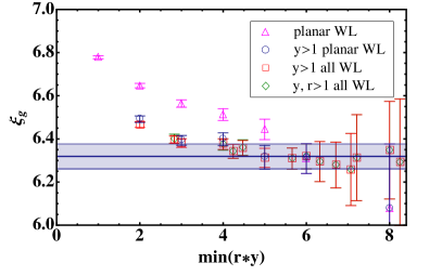
Figure 1: Gauge anisotropy $\xi_{g}$ obtained using $L(\xi_{g})$. Different colors denote different sets of Wilson loops used in the calculations as shown in the legend. The blue band is the extracted value of $\xi_{g}$ with the statistical uncertainty.

We determine the gauge anisotropy $\xi_{g}$ from the static potential measured by Wilson loops, which was first proposed by Klassen [8]. We introduce the ratios of spatial-spatial Wilson loops, $R_{s}(r,y)=W_{ss}(r,y)/W_{ss}(r+1,y)$, and spatial-temporal Wilson loops $R_{t}(r,t)=W_{st}(r,t)/W_{st}(r+1,t)$. The inter-quark potential at the same physical distance must have the same value, i.e. $R_{s}(r,y)=R_{t}(r,t=\xi_{g}y)$. In practice, we determine $\xi_{g}$ by minimizing $L(\xi_{g})=\sum_{r,y}\ell(\xi_{g};r,y)$ [9] with

$$\ell(\xi_{g})=\frac{(R_{s}(r,y)-R_{t}(r,\xi_{g}y))^{2}}{(\Delta R_{s})^{2}+(\Delta R_{t})^{2}},$$ (10)

where $\Delta R_{s}$ and $\Delta R_{t}$ are the statistical errors of $R_{s}$ and $R_{t}$, respectively. In this work we extend Klassen’s method by including nonplanar Wilson loops in which $r$ takes any two-dimentional paths in $x$-$z$ plane. To maximize the overlap with the physical ground state, we consider the path identified by $\vec{r}=(x,z)$ and $\vec{r}+1=(x+1,z)$ for fixed values of $z$. This modification allows us to secure enough data points before we encounter too large statistical errors as the size of Wilson loops increases, where we find a clean signal of the convergence of $\xi_{g}$ to its asymptotical value. The numerical results in Fig. 1 indeed show that $\xi_{g}$ reaches the plateau at around $\textrm{min}(r*y)=4\sim 6$. The largest systematic uncertainty occurs if we include the Wilson loops containing $y=1$, due to short-range lattice artefacts. In summary, the final values of $\xi_{g}$ is determined using planar and nonplanar Wilson loops, except the ones having $y=1$, at $\textrm{min}(r*y)=6$.

We determine the fermion anisotropy $\xi_{f}$ from the leading-order relativistic dispersion relation of mesons $E^{2}(p^{2})=M^{2}+p^{2}/\xi_{f}^{2}$ with $\vec{p}=2\pi\vec{n}/N_{s}$, where $M$ is the meson mass and $\vec{n}$ is the integer vector. Note that the energy and mass are in units of $a_{t}$ while the momentum is in units of $a_{s}$. For a given momentum $\vec{p}$, we measure the energy $E(p^{2})$ from a constant fit to the plateau of the effective mass $m_{\textrm{eff}}$ in the asymptotic region at a large time. We use point sources to construct the meson interpolating operators at source and sink, and consider the four lowest momentum vectors $\vec{n}=(0,0,0),\,(1,0,0),\,(0,1,0),\,(0,0,1)$ for the linear fit of $E^{2}(p^{2})$, where the resulting fit function reproduces well the large momentum states to $|{\vec{n}}|^{2}=3$. We also find that $\xi_{f}$ extracted from pseudoscalar mesons is in good agreement with that from vector mesons and shows better precision. Therefore, we use the former in the tuning of lattice bare parameters.

To determine the coefficients $a_{i}$, $b_{i}$, and $c_{i}$, we perform the simultaneous $\chi^{2}$ fit of the numerical data to the functions in Eq. (9). The results are

$$a_{0}=0.6(16),~{}a_{1}=0.97(13),~{}a_{2}=0.31(23),~{}a_{3}=2(4),$$

$$b_{0}=1.8(24),~{}b_{1}=0.06(18),~{}b_{2}=1.1(3),~{}b_{3}=4(7),$$

$$c_{0}=0.475(5),~{}c_{1}=-0.0168(4),~{}c_{2}=-0.0375(6),~{}c_{3}=0.986(11),$$ (11)

where the values of $\chi^{2}$ per degrees of freedom are $1.72$, $0.72$, $0.23$, respectively. These results show that the linear anzats in Eq. (9) work well over the range of considered lattice parameters.

To determine the critical values for the bare parameters we impose the following renormalization conditions:

$$\xi_{g}(\xi^{0*}_{g},\xi^{0*}_{f},m^{*}_{0})=\xi_{f}(\xi^{0*}_{g},\xi^{0*}_{f},m^{*}_{0})=\xi,~{}~{}~{}M^{2}_{PS}(\xi^{0*}_{g},\xi^{0*}_{f},m^{*}_{0})=m^{2}_{ps}.$$ (12)

Solving Eq. (9) with our target renormalized parameters of $\xi=6.3$ and $m_{ps}^{2}=0.005$, we find

$$\xi_{g}^{0*}=4.84(8),~{}\xi_{f}^{0*}=4.72(12),~{}m_{0}^{*}=-0.2148(37).$$ (13)

3.2 Numerical results at finite temperature

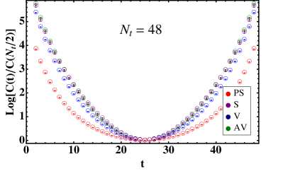
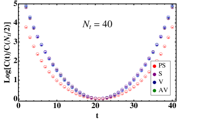
Figure 2: Temporal correlation functions of pseudo-scalar (red), scalar (purple), vector (blue), and axial-vector (green) mesons, normalized by those at $N_{t}/2$.

Finite $T$ calculations are performed on the anisotropic lattices of $N_{t}\times 16^{3}$ with $N_{t}=16,\,20,\,24$, $28,\,30,\,36,\,40,\,128$, and $N_{t}\times 16^{2}\times 24$ with $N_{t}=8,\,12,\,16,\,20,\,24,\,28,\,36,\,42,\,48,\,56$. The lattice parameters are taken from the central values in Eq. (13), namely $\xi_{g}^{0}=4.84,~{}\xi_{f}^{0}=4.72,~{}m_{0}=-0.2148$. Throughout this work, we measure $T$ in units of the pseudo-critical temperature $T_{c}$. Following the procedure described in [10] , we determine $T_{c}$ using the renormalized Polyakov loop $L_{R}$ as an indication of the deconfinement crossover. For the determination, we consider three renormaliztion conditions, $L_{R}(N_{t}=24)=0.9,~{}L_{R}(N_{t}=24)=0.5$, and $L_{R}(N_{t}=20)=0.9$. From the peak of the susceptibility, $\chi(L_{R})=\partial L_{R}/\partial T$, we find that $T_{c}a_{t}=0.0255(25)$ or equivalently $N_{t}^{c}=39(4)$. The statistical and systematic (scheme dependence) uncertainties are combined in quadrature.

We consider flavored pseudo-scalar, scalar, vector, and axial-vector mesons, where the corresponding interpolating fields are defined by

$$\mathcal{O}_{PS}(x)=\bar{q}(x)\gamma_{5}q(x),~{}\mathcal{O}_{S}(x)=\bar{q}(x)q(x),$$

$$\mathcal{O}_{V}^{i}(x)=\bar{q}(x)\gamma^{i}q(x),~{}\mathcal{O}_{AV}^{i}(x)=\bar{q}(x)\gamma_{5}\gamma^{i}q(x),$$ (14)

respectively. To improve the statistics, we use stochastic wall sources [11] for the study of meson spectra. At finite temperature the spectral function of mesons no longer exhibits a sharp peak at the mass of mesons, which makes it difficult to measure the mass from the single exponential analysis of a two-point function. In this case, it is more desirable to investigate the correlation functions by themselves. In Fig. 2 we show the temporal correlation functions $C(t)$ for $N_{t}=48$ and $N_{t}=40$, which exemplify the typical behaviors of $C(t)$ below and at the critical temperature, respectively. The overlap of $C(t)$ between vector and axial-vector mesons appears at the critical temperature supporting the restoration of the $SU(4)$ global symmetry.

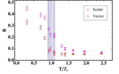
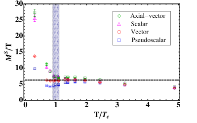
Figure 3: Mass ratios $R$ defined in the text (left) and meson screening masses normalized by the temperature (right). The temperature is in units of $T_{c}$. The vertical blue bands denote the uncertainty of $T_{c}$. The black dashed line at $2\pi$ corresponds to the Matsubara frequency — the lowest excitation with free particles.

In contrast to the temporal correlation function, the spatial correlation function at finite temperature exhibits a single exponential decay at large time. The decay rate is the screening mass that defines the effective length scale associated with the excitation of mesonic operators in the medium [12]. The screening mass is equivalent to the meson mass at zero temperature, as the temporal and spatial correlation functions share the same spectral function. Using the meson interpolating fields in Eq. (14), we measure the screening masses from spatial correlators along $z$-direction $C(z)$.

In addition to the screening masses, we define the mass ratios as

$$R_{V(S)}(T)=\frac{M_{AV(S)}(T)-M_{V(PS)}(T)}{M_{AV(S)}(T)+M_{V(PS)}(T)}.$$ (15)

These quantities are useful to quantify the size of deviation from the parity doubled states. Our main results are presented in Fig. 3. No significant excited state contaminations appear to spoil the good agreement between results from $N_{z}=16$ and $N_{z}=24$ lattices. Although there is small deviation from zero in the mass ratio, the plateau above $T_{c}$ in the vector channel would suggest that parity partners are degenerate and thus the symmetry is effectively enhanced to $SU(4)$. In the scalar channel, the plateau appears at a somewhat larger temperature $\sim 1.5\,T_{c}$. This result may imply that the $U(1)_{A}$ symmetry and $SU(4)$ symmetry are restored at different temperature. This might be an indication that instead of a phase transition a crossover between two different regimes is taking place.

In the finite temperature calculations, it is often suggested to plot the screening masses divided by the temperature as it shows linear dependency above $T_{c}$. The results are shown in Fig. 3, where those quantities approach the black dashed line at around $T_{c}$ and form a plateau. However, they start to deviate from the plateau above $2T_{c}$ due to the lattice artefacts (finite lattice spacing).

4 Conclusion

We considered $SU(2)$ gauge theory with $N_{f}=2$ flavors of fundamental Dirac fermions. The symmetry breaking $SU(4)\rightarrow Sp(4)$ is responsible for the mass splitting of flavored vector and axial-vector mesons, while the anomalous $U(1)_{A}$ breaking splits scalar and pseudo-scalar mass spectra. In the thermal bath, one expects the restoration of the global symmetries. We measured the meson spectra via Monte-Carlo simulations on anisotropic lattices and indeed found strong evidence of the enhancement of the global symmetry above the temperature $T_{c}$, as shown in Fig. 3.

We only considered a single value of lattice spacing and quark mass. In future works we plan to extend our study by using various choices of lattice spacings and quark masses to assess the size of lattice systematics. Another interesting direction for the future is to simulate the model with a non-zero chemical potential, taking advantage of the absence of the sign problem.

5 Acknowledgements

This work is supported in part by the STFC Consolidated Grant ST/L000369/1. J.-W. L. is additionally supported by Korea Research Fellowship program funded by the Ministry of Science, ICT and Future Planning through the National Research Foundation of Korea (2016HID3A1909283). The authors thank S. Hands, G. Aarts, B. Jäger, F. Attanasio and E. Bennett for discussions.

References

- [1] T. Boz, S. Cotter, L. Fister, D. Mehta and J.-I. Skullerud, Eur. Phys. J. A 49, 87 (2013).
- [2] G. Cacciapaglia and F. Sannino, JHEP 1404, 111 (2014).
- [3] R. Lewis, C. Pica and F. Sannino, Phys. Rev. D 85, 014504 (2012).
- [4] J.-W. Lee, B. Lucini and M. Piai, arXiv:1701.03228 [hep-lat] (2017).
- [5] L. Del Debbio, A. Patella and C. Pica, Phys. Rev. D 81, 094503 (2010).
- [6] R. Morrin, A. O. Cais, M. Peardon, S. M. Ryan and J.-I. Skullerud, Phys. Rev. D 74, 014505 (2006).
- [7] R. G. Edwards, B. Joo and H.-W. Lin, Phys. Rev. D 78, 054501 (2008).
- [8] T. R. Klassen, Nucl. Phys. B 533, 557-575 (1998).
- [9] T. Umeda et al. (CP-PACS), Phys. Rev. D 68 034503 (2003).
- [10] G. Aarts, C. Allton, A. Amato, P. Giudice, S. Hands and J.-I. Skullerud, JHEP 02, 186 (2015).
- [11] P. A. Boyle, A. Juttner, C. Kelly and R. D. Kenway, JHEP 0808, 086, (2008).
- [12] C. DeTar and J. B. Kogut, Phys. Rev. Lett. 59, 399 (1987), Phys. Rev. D 36 2828 (1987).