Learning Hierarchical Features from Generative Models

Abstract

Deep neural networks have been shown to be very successful at learning feature hierarchies in supervised learning tasks. Generative models, on the other hand, have benefited less from hierarchical models with multiple layers of latent variables. In this paper, we prove that hierarchical latent variable models do not take advantage of the hierarchical structure when trained with existing variational methods, and provide some limitations on the kind of features existing models can learn. Finally we propose an alternative architecture that do not suffer from these limitations. Our model is able to learn highly interpretable and disentangled hierarchical features on several natural image datasets with no task specific regularization or prior knowledge.

1 Introduction

A key property of deep feed-forward networks is that they tend to learn learn increasingly abstract and invariant representations at higher levels in the hierarchy (Bengio, 2009; Zeiler & Fergus, 2014) In the context of image data, low levels may learn features corresponding to edges or basic shapes, while higher levels learn more abstract features, such as object detectors (Zeiler & Fergus, 2014).

Generative models with a hierarchical structure, where there are multiple layers of latent variables, have been less successful compared to their supervised counterparts (Sønderby et al., 2016). In fact, the most successful generative models often use only a single layer of latent variables (Radford et al., 2015; van den Oord et al., 2016), and those that use multiple layers only show modest performance increases in quantitative metrics such as log-likelihood (Sønderby et al., 2016; Bachman, 2016). Because of the difficulties in evaluating generative models (Theis et al., 2015), and the fact that adding network layers increases the number of parameters, it is not always clear whether the improvements truly come from the choice of a hierarchical architecture. Furthermore, the capability of learning a hierarchy of increasingly complex and abstract features has only been demonstrated to a limited extent, with feature hierarchies that are not nearly as rich as the ones learned by feed-forward networks (Gulrajani et al., 2016).

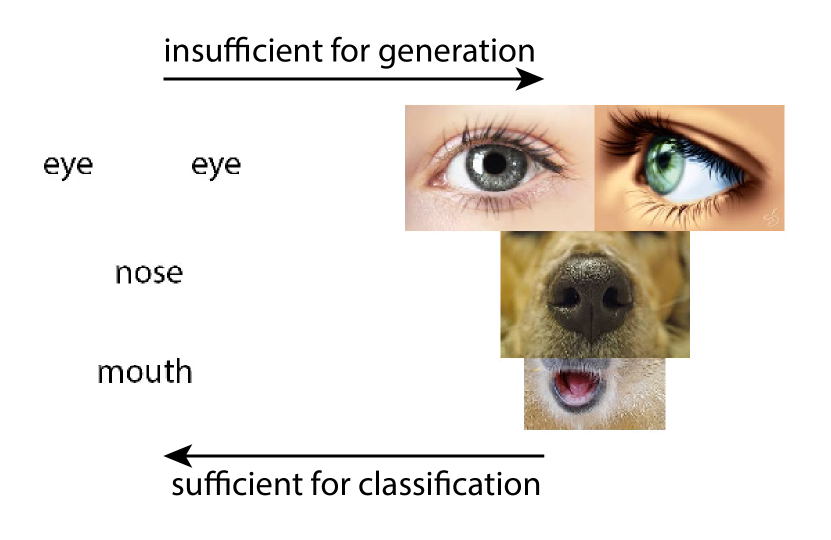
Figure 1: Left: Body parts feature detectors only carry a small amount of information about an underlying image, yet, it is sufficient for a confident classification as a face. Right: if a hierarchical generative model attempts to reconstruct an image based on these high-level features, it could generate inconsistent images, even when each part can be perfectly generated. Even though this ”face” is clearly absurd, Google cloud platform classification API can identify with 93% confidence that this is a face.

Part of the problem is inherent and unavoidable for any generative model. The heart of the matter is that while highly invariant and local features are often sufficient for classification, generative modeling requires preservation of details (as illustrated in Figure 1). In fact, most latent features in a generative model of images cannot even demonstrate scale and translation invariance. The size and location of a sub-part often has to be dependent on the other sub-parts. For example, an eye should only be generated with the same size as the other eye, at symmetric locations with respect to the center of the face, with appropriate distance between them. The inductive biases that are directly encoded into the architecture of convolutional networks is not sufficient in the context of generative models.

On the other hand, other problems are associated with specific models or design choices, and may be avoided with deeper understanding and careful design. The goal of this paper is to provide a deeper understanding of the design and performance of common hierarchical latent variable models. We focus on variational models, though most of the conclusions can be generalized to adversarially trained models that support inference (Dumoulin et al., 2016; Donahue et al., 2016). In particular, we study two classes of models with a hierarchical structure:

1) Stacked hierarchy: The first type we study is characterized by recursively stacking generative models on top of each other. Most existing models (Sønderby et al., 2016; Gulrajani et al., 2016; Bachman, 2016; Kingma et al., 2016), belong to this class. We show that these models have two limitations. First, we show that if these models can be trained to optimality, then the bottom layer alone contains enough information to reconstruct the data distribution, and the layers above the first one can be ignored. This result holds under fairly general conditions, and does not depend on the specific family of distributions used to define the hierarchy (e.g., Gaussian). Second, we argue that many of the building blocks commonly used to construct hierarchical generative models are unlikely to help us learn disentangled features.

2) Architectural hierarchy: Motivated by these limitations, we turn our attention to single layer latent variable models. We propose an alternative way to learn disentangled hierarchical features by crafting a network architecture that prefers to place high-level features on certain parts of the latent code, and low-level features in others. We show that this approach, called Variational Ladder Autoencoder, allows us to learn very rich feature hierarchies on natural image datasets such as MNIST, SVHN  (Netzer et al., 2011) and CelebA  (Liu et al., 2015); in contrast, generative models with a stacked hierarchical structure fail to learn such features.

2 Problem Setting

We consider a family of latent variable models specified by a joint probability distribution $p_{\theta}({{\bf x}},{{\bf z}})$ over a set of observed variables ${{\bf x}}$ and latent variables ${{\bf z}}$. The family of models is assumed to be parametrized by $\theta$. Let $p_{\theta}({{\bf x}})$ denote the marginal distribution of ${{\bf x}}$. We wish to maximize the marginal log-likelihood $p({{\bf x}})$ over a dataset ${{\bf X}}=\{{{\bf x}}^{(1)},\ldots,{{\bf x}}^{(N)}\}$ drawn from some unknown underlying distribution $p_{data}({{\bf x}})$. Formally we would like to maximize

$$\log p_{\theta}({{\bf X}})=\sum_{n=1}^{N}\log p_{\theta}({{\bf x}}^{(i)})$$ (1)

which is non-convex and often intractable for complex generative models, as it involves marginalization over the latent variables ${{\bf z}}$.

We are especially interested in unsupervised feature learning applications, where by maximizing (1) we hope to discover a meaningful representation for the data ${{\bf x}}$ in terms of latent features given by $p_{\theta}({{\bf z}}|{{\bf x}})$.

2.1 Variational Autoencoders

A popular solution (Kingma & Welling, 2013; Jimenez Rezende et al., 2014) for optimizing the intractable marginal likelihood (1) is to optimize the evidence lower bound (ELBO) by introducing an inference model $q_{\phi}({{\bf z}}\lvert{{\bf x}})$ parametrized by $\phi$ :

$$\log p({{\bf x}}) \geq\mathbb{E}_{q({{\bf z}}\lvert{{\bf x}})}[\log p({{\bf x}},{{\bf z}})-\log q({{\bf z}}\lvert{{\bf x}})]$$

$$=\mathbb{E}_{q({{\bf z}}|{{\bf x}})}[\log p({{\bf x}}|{{\bf z}})]-\mathbb{KL}(q({{\bf z}}\lvert{{\bf x}})\lVert p({{\bf z}}))$$

$$=\mathcal{L}({{\bf x}};\theta,\phi)$$ (2)

where $\mathbb{KL}$ is the Kullback-Leibler divergence.

2.2 Hierarchical Variational Autoencoders

A hierarchical VAE (HVAE) can be thought of as a series of VAEs stacked on top of each other. It has the following hierarchy of latent variables ${{\bf z}}=\{{{\bf z}}_{1},\ldots,{{\bf z}}_{L}\}$, in addition to the observed variables ${{\bf x}}$. We use the notation convention that ${{\bf z}}_{1}$ represents the lowest layer closest to ${{\bf x}}$ and ${{\bf z}}_{L}$ the top layer. Using chain rule, the joint distribution $p({{\bf x}},{{\bf z}}_{1},\ldots,{{\bf z}}_{L})$ can be factored as follows

$$p({{\bf x}},{{\bf z}}_{1},\ldots,{{\bf z}}_{L})=p({{\bf x}}\lvert{{\bf z}}_{>0})\prod_{\ell=1}^{L-1}p({{\bf z}}_{\ell}\lvert{{\bf z}}_{>\ell})p({{\bf z}}_{L})$$ (3)

where ${{\bf z}}_{>\ell}$ indicates $({{\bf z}}_{\ell+1},\cdots,{{\bf z}}_{L})$, and ${{\bf z}}_{>0}={{\bf z}}=({{\bf z}}_{1},\ldots,{{\bf z}}_{L})$. Note that this factorization via chain-rule is fully general. In particular it accounts for recent models that use shortcut connections (Kingma et al., 2016; Bachman, 2016), where each hidden layer ${{\bf z}}_{\ell}$ directly depends on all layers above it (${{\bf z}}_{>\ell}$). We shall refer to this fully general formulation as autoregressive HVAE.

Several models assume a Markov independence structure on the hidden variables, leading to the following simpler factorization (Jimenez Rezende et al., 2014; Gulrajani et al., 2016; Kaae Sønderby et al., 2016)

$$p({{\bf x}},{{\bf z}})=p({{\bf x}}|{{\bf z}}_{\ell})\prod_{l=1}^{L-1}p({{\bf z}}_{\ell}|{{\bf z}}_{\ell+1})p({{\bf z}}_{L})$$ (4)

We refer to this common but more restrictive formulation as Markov HVAE.

For the inference distribution $q({{\bf z}}|{{\bf x}})$ we do not assume any factorized structure to account for complex inference techniques used in recent work (Kaae Sønderby et al., 2016; Bachman, 2016). We also denote $q({{\bf x}},{{\bf z}})=p_{data}({{\bf x}})q({{\bf z}}|{{\bf x}})$.

Both $p({{\bf x}}|{{\bf z}})$ and $q({{\bf z}}|{{\bf x}})$ are jointly optimized, as before in Equation (2), to maximize the ELBO objective

$$\mathcal{L}_{ELBO} =E_{p_{data}({{\bf x}})}E_{q({{\bf z}}|{{\bf x}})}[\log p({{\bf x}}|{{\bf z}})]-$$

$$\qquad\qquad E_{p_{data}({{\bf x}})}[\mathbb{KL}(q({{\bf z}}|{{\bf x}})||p({{\bf z}}))]$$

$$=\sum_{l=0}^{L}E_{q({{\bf z}},{{\bf x}})}[\log p({{\bf z}}_{l}|{{\bf z}}_{>l})]+H(q({{\bf z}}|{{\bf x}}))$$ (5)

where we define ${{\bf z}}_{0}\equiv{{\bf x}}$, ${{\bf z}}_{L+1}\equiv{\bf 0}$, and $H$ the entropy of a distribution, and expectation over $p_{data}(x)$ is estimated by the samples in the dataset. This can be interpreted as stacking VAEs on top of each other.

3 Limitations of Hierarchical VAEs

3.1 Representational Efficiency

One of the main reasons deep hierarchical networks are widely used as function approximators is their representational power. It is well known that certain functions can be represented much more compactly with deep networks, requiring exponentially less parameters compared to shallow networks (Bengio et al., 2009). However, we show that under ideal optimization of $\mathcal{L}_{ELBO}$, HVAE models do not lead to improved representational power. This is because for a well trained HVAE, a Gibbs chain on the bottom layer, which is a single layer model, can be used to recover $p_{data}({{\bf x}})$ exactly.

We first show this formally for Markov HVAE with the following proposition

Proposition 1.

$\mathcal{L}_{ELBO}$ in Eq.(5) is globally maximized as a function of $q({{\bf z}}|{{\bf x}})$ and $p({{\bf x}}|{{\bf z}})$ when $\mathcal{L}_{ELBO}=-H(p_{data}(x))$. If $\mathcal{L}_{ELBO}$ is globally maximized for a Markov HVAE, the following Gibbs sampling chain converges to $p_{data}({{\bf x}})$ if it is ergodic

$${{\bf z}}_{1}^{(t)} \sim q({{\bf z}}_{1}|{{\bf x}}^{(t)})$$

$${{\bf x}}^{(t+1)} \sim p({{\bf x}}|{{\bf z}}_{1}^{(t)})$$ (6)

Proof of Proposition 1.

We notice that

$$\mathcal{L}_{ELBO}=E_{p_{data}({{\bf x}})q({{\bf z}}|{{\bf x}})}\left[\log\frac{p({{\bf x}},{{\bf z}})}{q({{\bf z}}|{{\bf x}})}\right]$$

$$\qquad=E_{p_{data}({{\bf x}})q({{\bf z}}|{{\bf x}})}\left[\log\frac{p({{\bf z}}|{{\bf x}})}{q({{\bf z}}|{{\bf x}})}\right]+E_{p_{data}({{\bf x}})}[\log p({{\bf x}})]$$

$$\qquad=-E_{p_{data}({{\bf x}})}[\mathbb{KL}(q({{\bf z}}|{{\bf x}})||p({{\bf z}}|{{\bf x}}))]$$

$$\qquad\qquad-\mathbb{KL}(p_{data}({{\bf x}})||p({{\bf x}}))-H(p_{data}({{\bf x}}))$$

By non-negativity of KL-divergence, and the fact that KL divergence is zero if an only if the two distributions are identical, it can be seen that this is uniquely optimized when $p({{\bf x}})=\int_{{\bf z}}p({{\bf x}},{{\bf z}})d{{\bf z}}=p_{data}({{\bf x}})$ and $\forall{{\bf x}},q({{\bf z}}|{{\bf x}})=p({{\bf z}}|{{\bf x}})$ and the optimum is

$$\mathcal{L}^{*}_{ELBO}=-H(p_{data}({{\bf x}}))$$

This also implies that $\forall{{\bf x}}$

$$q({{\bf x}}|{{\bf z}}_{1})=\frac{q({{\bf z}}_{1}|{{\bf x}})p_{data}({{\bf x}})}{q({{\bf z}}_{1})}=p({{\bf x}}|{{\bf z}}_{1})$$ (7)

Because the following Gibbs chain converges to $p_{data}({{\bf x}})$ when it is ergodic

$${{\bf z}}_{1}^{(t)} \sim q({{\bf z}}_{1}|{{\bf x}}^{(t)})$$

$${{\bf x}}^{(t+1)} \sim q({{\bf x}}|{{\bf z}}_{1}^{(t)})$$

We can replace $q({{\bf x}}|{{\bf z}}_{1}^{(t)})$ with $p({{\bf x}}|{{\bf z}}_{1}^{(t)})$ using (7) and the chain still converges to $p_{data}({{\bf x}})$. ∎

Therefore under the assumptions of Proposition 1 we can sample from $p_{data}({{\bf x}})$ without using the latent code $({{\bf z}}_{2},\cdots,{{\bf z}}_{L})$ at all. Hence, optimization of the $\mathcal{L}_{ELBO}$ objective and efficient representation are conflicting, in the sense that optimality implies some level of redundancy in the representation.

We demonstrate that this phenomenon occurs in practice, even though the conditions of Proposition 1 might not be met exactly. We train a factorized three layer VAE in Equation (4) on MNIST by optimizing the ELBO criteria Equation (5). We use a model where each conditional distribution is factorized Gaussian $p({{\bf z}}_{\ell}|{{\bf z}}_{\ell+1})=\mathcal{N}(\mu_{\ell}({{\bf z}}_{\ell+1}),\sigma_{\ell}({{\bf z}}_{\ell+1}))$ where $\mu_{\ell}$ and $\sigma_{\ell}$ are deep networks. We compare: the samples generated by the Gibbs chain in Equation (6) with samples generated by ancestral sampling with the entire model in Figure 2. We observe that the Gibbs chain generates samples (left panel) with similar visual quality as ancestral sampling with the entire model (right panel), even though the Gibbs chain only used the bottom layer of the model.

This problem can be generalized to autoregressive HVAEs. One can sample from $p_{data}({{\bf x}})$ without using $p({{\bf z}}_{\ell}|{{\bf z}}_{>\ell}),1\leq\ell<L$ at all. We prove this in the Appendix.

3.2 Feature learning

Another significant advantage of hierarchical models for supervised learning is that they learn rich and disentangled hierarchies of features. This has been demonstrated for example using various visualization techniques (Zeiler & Fergus, 2014). However, we show in this section that typical HVAEs do not enjoy this property.

Recall that we think of $p({{\bf z}}|{{\bf x}})$ as a (probabilistic) feature detector, and $q({{\bf z}}|{{\bf x}})$ as an approximation to $p({{\bf z}}|{{\bf x}})$. It might therefore be natural to think that $q$ might learn hierarchical features similarly to a feed-forward network $x\to{{\bf z}}_{\ell}\to\cdots\to{{\bf z}}_{L}$, where higher layers correspond to higher level features that become increasingly abstract and invariant to nuisance variations. However if $q({{\bf z}}_{>\ell}|{{\bf z}}_{\ell})$ maps low level features to high level features, then the reverse mapping $q({{\bf z}}_{\ell}|{{\bf z}}_{>\ell})$ maps high level features to likely low level sub-features. For example, if ${{\bf z}}_{L}$ correspond to object classes, then $q({{\bf z}}_{L-1}|{{\bf z}}_{L})$ could represent the distribution over object subparts given the object class.

Suppose we train $\mathcal{L}_{ELBO}$ in Equation (5) to optimality, we would have

$$p({{\bf x}})=p_{data}({{\bf x}}),q({{\bf z}}|{{\bf x}})=p({{\bf z}}|{{\bf x}})$$

Recall that

$$q({{\bf x}},{{\bf z}}) :=p_{data}({{\bf x}})q({{\bf z}}|{{\bf x}})$$

$$p({{\bf x}},{{\bf z}}) :=p({{\bf z}})p({{\bf x}}|{{\bf z}})=p({{\bf x}})p({{\bf z}}|{{\bf x}})$$

Comparing the two we see that

$$p({{\bf x}},{{\bf z}})=q({{\bf x}},{{\bf z}})$$

if the joint distributions are identical, then any conditional distribution would also be identical, which implies that for any ${{\bf z}}_{>\ell}$, $q({{\bf z}}_{\ell}|{{\bf z}}_{>\ell})=p({{\bf z}}_{\ell}|{{\bf z}}_{>\ell})$.

For the majority of models the conditional distributions $p({{\bf z}}_{\ell}|{{\bf z}}_{>\ell})$ belong to a very simple distribution family such as parameterized Gaussians (Kingma & Welling, 2013) (Jimenez Rezende et al., 2014) (Kaae Sønderby et al., 2016) (Kingma et al., 2016). Therefore for a perfectly optimized $\mathcal{L}_{ELBO}$ in the Gaussian case, the only type of feature hierarchy we can hope to learn is one under which $q({{\bf z}}_{\ell}|{{\bf z}}_{>\ell})$ is also Gaussian. This limits the hierarchical representation we can learn. In fact, the hierarchies we observe for feed-forward models (Zeiler & Fergus, 2014) require complex multimodal distributions to be captured. For example, the distribution over object subparts for an object category is unlikely to be unimodal and cannot be well approximated with a Gaussian distribution.

More generally, as shown in (Zhao et al., 2017), even when $\mathcal{L}_{ELBO}$ is not globally optimized, optimizing $\mathcal{L}_{ELBO}$ encourages $q({{\bf z}}_{\ell}|{{\bf z}}_{>\ell})$ and $p({{\bf z}}_{\ell}|{{\bf z}}_{>\ell})$ to match. Because $p({{\bf z}}_{\ell}|{{\bf z}}_{>\ell})$ belong to some distribution family, such as Gaussians. This encourages $q({{\bf z}}_{\ell}|{{\bf z}}_{>\ell})$ to belong to that distribution family as well.

We experimentally demonstrate these intuitions in Figure 3, where we train a three layer Markov HVAE with factorized Gaussian conditionals $p({{\bf z}}_{\ell}|{{\bf z}}_{\ell+1})$ on MNIST and SVHN. Details about the experimental setup are explained in the Appendix. As suggested in (Kingma & Welling, 2013), we reparameterize the stochasticity in $p({{\bf z}}_{\ell}|{{\bf z}}_{\ell+1})$ using a separate noise variable ${\bm{\epsilon}}_{\ell}\sim\mathcal{N}(0,I)$, and implicitly rewrite the original conditional distribution as

$${{\bf z}}_{\ell}=\mu_{\ell}({{\bf z}}_{\ell+1})+\sigma_{\ell}({{\bf z}}_{\ell+1})\odot{\bm{\epsilon}}_{\ell}$$

where $\odot$ indicates element-wise product. We fix the value of ${\bm{\epsilon}}_{k}$ to a random sample from $\mathcal{N}(0,I)$ at all layers $k=1,\cdots,\ell-1,\ell+1,\cdots,L$ except for one, and observe the variations in ${{\bf x}}$ generated by randomly sampling ${\bm{\epsilon}}_{\ell}$. We observe in Figure 3 that only very minor variations correspond to lower layers (Left and center panels), and almost all the variation is represented by the top layer (Right panel). More importantly, no notable hierarchical relationship between features is observed.

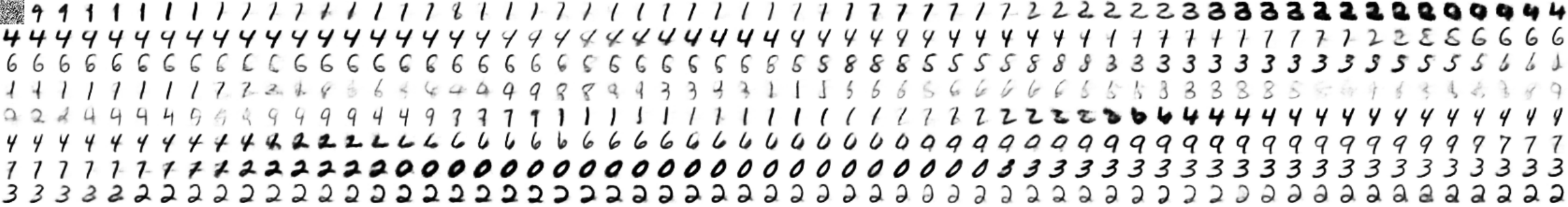
Figure 2: Left: Samples obtained by running the Gibbs sampling chain in Proposition 1, using only the bottom layer of a 3-layer recursive hierarchical VAE. Right: samples generated by ancestral sampling from the same model. The quality of the samples is comparable, indicating that the bottom layer contains enough information to reconstruct the data distribution.

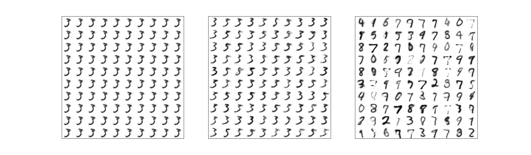
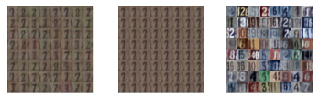
Figure 3: A hierarchical three layer VAE with Gaussian conditional distributions $p({{\bf z}}_{l}|{{\bf z}}_{l+1})$ does not learn a meaningful feature hierarchy on MNIST and SVHN when trained with the ELBO objective. Left panel: Samples generated by sampling noise ${\bm{\epsilon}}_{1}$ at the bottom layer, while holding ${\bm{\epsilon}}_{2}$ and ${\bm{\epsilon}}_{3}$ constant. Center panel: Samples generated by sampling noise ${\bm{\epsilon}}_{2}$ at the middle layer, while holding ${\bm{\epsilon}}_{1}$ and ${\bm{\epsilon}}_{3}$ constant. Right panel: Samples generated by sampling noise ${\bm{\epsilon}}_{3}$ at the top layer, while holding ${\bm{\epsilon}}_{1}$ and ${\bm{\epsilon}}_{2}$ constant. For both MNIST and SVHN we observe that the top layer represents essentially all the variation in the data (right panel), leaving only very minor local variations for the lower layers (left and center panels). Compare this with the rich hierarchy learned by our VLAE model, shown in Figures 5 and 6.

4 Variational Ladder Autoencoders

Given the limitations of hierarchical architectures described in the previous section, we focus on an alternative approach to learn a hierarchy of disentangled features.

Our approach is to define a simple distribution with no hierarchical structure over the latent variables $p({{\bf z}})=p({{\bf z}}_{1},\cdots,{{\bf z}}_{L})$. For example, the joint distribution $p({{\bf z}})$ can be a white Gaussian. Instead we encourage the latent code ${{\bf z}}_{1},\cdots,{{\bf z}}_{L}$ to learn features with different levels of abstraction by carefully choosing the mappings $p({{\bf x}}|{{\bf z}})$ and $q({{\bf z}}|{{\bf x}})$ between input ${{\bf x}}$ and latent code ${{\bf z}}$. Our approach is based on the following intuition:

Assumption: If ${{\bf z}}_{i}$ is more abstract than ${{\bf z}}_{j}$, then the inference mapping $q({{\bf z}}_{i}|{{\bf x}})$ and generative mapping when other layers are fixed $p({{\bf x}}|{{\bf z}}_{i},{{\bf z}}_{\neg i}=z^{0}_{\neg_{i}})$ requires a more expressive network to capture.

This informal assumption suggests that we should use neural networks of different level of expressiveness to generate the corresponding features; the more abstract features require more expressive networks, and vice versa. We loosely quantify expressiveness with depth of the network. Based on these assumptions we are able to design an architecture that disentangles hierarchical features for many natural image datasets.

4.1 Model Definition

We decompose the latent code into subparts ${{\bf z}}=\{{{\bf z}}_{1},{{\bf z}}_{2},\ldots\}$, where ${{\bf z}}_{1}$ relates to ${{\bf x}}$ with a shallow network, and increase network depth up to ${{\bf z}}_{L}$, which relates to ${{\bf x}}$ with a deep network. In particular, we share parameters with a ladder-like architecture (Valpola, 2015; Pezeshki et al., 2015). Because of this similarity we denote this architecture as Variational Ladder Autoencoder (VLAE). Formally, our model, shown in Figure 4 is defined as follows

1) Generative Network: $p({{\bf z}})=p({{\bf z}}_{1},\cdots,{{\bf z}}_{L})$ is a simple prior on all latent variables. We choose it as a standard Gaussian $\mathcal{N}(0,I)$. The conditional distribution $p({{\bf x}}|{{\bf z}}_{1},{{\bf z}}_{2},\ldots,{{\bf z}}_{L})$ is defined implicitly as:

$$\tilde{{{\bf z}}}_{L} ={{\bf f}}_{L}({{\bf z}}_{L})$$ (8)

$$\tilde{{{\bf z}}}_{\ell} ={{\bf f}}_{\ell}(\tilde{{{\bf z}}}_{\ell+1},{{\bf z}}_{\ell})\ \ \ \ell=1,\cdots,L-1$$ (9)

$${{\bf x}} \sim{{\bf r}}({{\bf x}};{{\bf f}}_{0}(\tilde{{{\bf z}}}_{1}))$$ (10)

where ${{\bf f}}_{\ell}$ is parametrized as a neural network, and $\tilde{{{\bf z}}}_{\ell}$ is an auxiliary variable we use to simplify the notation. ${{\bf r}}$ is a distribution family parameterized by ${{\bf f}}_{0}(\tilde{{{\bf z}}}_{1})$. In our experiments we use the following choice for ${{\bf f}}_{\ell}$:

$$\tilde{{{\bf z}}}_{\ell} ={{\bf u}}_{\ell}([\tilde{{{\bf z}}}_{\ell+1};{{\bf v}}_{\ell}({{\bf z}}_{\ell})])$$ (11)

where $[\cdot;\cdot]$ denotes concatenation of two vectors, and ${{\bf v}}_{\ell},{{\bf u}}_{\ell}$ are neural networks. We choose ${{\bf r}}$ as a fixed variance factored Gaussian with mean given by ${\bm{\mu}}_{r}={{\bf f}}_{0}(\tilde{{{\bf z}}}_{1})$.

2) Inference Network: For the inference network, we choose $q({{\bf z}}\lvert{{\bf x}})$ as

$${{\bf h}}_{\ell} ={{\bf g}}_{\ell}({{\bf h}}_{\ell-1})$$ (12)

$${{\bf z}}_{\ell} \sim\mathcal{N}({\bm{\mu}}_{\ell}({{\bf h}}_{\ell}),{\bm{\sigma}}_{\ell}({{\bf h}}_{\ell}))$$ (13)

where $\ell=1,\cdots,L$, ${{\bf g}}_{\ell}$, ${\bm{\mu}}_{\ell}$, ${\bm{\sigma}}_{\ell}$ are neural networks, and ${{\bf h}}_{0}\equiv{{\bf x}}$.

3) Learning: For learning we use the ELBO criteria as in Equ.(2):

where $p({{\bf z}})=\mathcal{N}(0,{{\bf I}})$ denotes the prior for ${{\bf z}}$. This is tractable if ${{\bf r}}$ has tractable log likelihood, i.e. when ${{\bf r}}$ is a Gaussian.

This is essentially the inference and learning framework for a one-layer VAE; the hierarchy is only implicitly defined by the network architecture, therefore we call this model flat hierarchy. Motivated by our earlier theoretical results, we do not use additional layers of latent variables.

4.2 Comparison with Ladder Variational Autoencoders

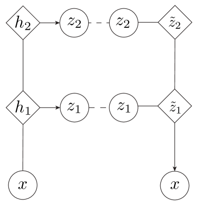
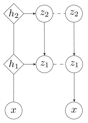
Figure 4: Inference and generative models for VLAE (left) and LVAE (right). Circles indicate stochastic nodes, and squares are deterministically computed nodes. Solid lines with arrows denote conditional probabilities; solid lines without arrows denote deterministic mappings; dash lines indicates regularization to match the prior $p({{\bf z}})$. Note that in VLAE, we do not attempt to regularize the distance between ${{\bf h}}$ and $\tilde{{{\bf z}}}$.

Our architecture resembles the ladder variational autoencoder (LVAE) (Sønderby et al., 2016). However the two models are very different. The purpose of our architecture is to connect subparts of the latent code with networks of different expressive power (depth); the model is encouraged to place high-level, complex features at the top, and low-level, simple features at the bottom, in order to reach lower reconstruction error with latent codes of the same capacity. Empirically, this allows the network to learn disentangled factors of variation, corresponding to different subparts of the latent code. Meanwhile, because it is essentially a single-layer flat model, our VLAE does not exhibit the problems we have identified with traditional hierarchical VAE described in Section 3.

Ladder Variational Autoencoders (LVAE) on the other hand, utilize the ladder architecture from the inference/encoding side; its generative model is a standard HVAE. While the ladder inference network performs better than the one used in the original HVAE, ladder variational autoencoders still suffer from the problems we discussed in Section 3. The difference is between our model (VLAE) and LVAE is illustrated in Figure 4

An additional advantage over ladder variational autoencoders (and more generally HVAEs) is that our definition of the generative network Equ.(10) allows us to select a much richer family of generative models $p$. Because for HVAE the $\mathcal{L}_{ELBO}$ optimization requires the evaluation of $\log p({{\bf z}}_{\ell}|{{\bf z}}_{\ell+1})$ shown in Equ.(5), a reparameterized HVAE inject noise into the network in a way that corresponds to a conditional distribution with a tractable log-likelihood. For example, a HVAE can inject noise ${\bm{\epsilon}}_{\ell}$ by

$${{\bf z}}_{\ell}={\bm{\mu}}_{\ell}({{\bf z}}_{\ell+1})+{\bm{\sigma}}_{\ell}({{\bf z}}_{\ell+1})\odot{\bm{\epsilon}}_{\ell}$$ (15)

only because this corresponds to Gaussian conditional distributions $p({{\bf z}}_{l}|{{\bf z}}_{l+1})$. In comparison, for VLAE we only require evaluation of $\log p({{\bf x}}|{{\bf z}}_{1},\cdots,{{\bf z}}_{L})$, so except for the bottom layer ${{\bf r}}$ we can combine noise by any arbitrary black box function ${{\bf f}}_{\ell}$.

5 Experiments

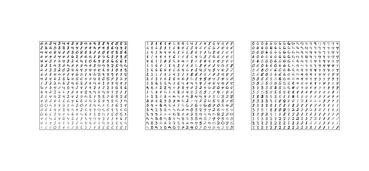
Figure 5: VLAE on MNIST. Generated digits obtained by systematically exploring the 2D latent code from one layer, and randomly sampling from other layers. Left panel: The first (bottom) layer encodes stroke width, Center panel: the second layer encodes digit width and tilt, Right panel: the third layer encodes (mostly) digit identity. Note that the samples are not of state-of-the-art quality only because of the restricted 2-dimensional latent code used to enable visualization.

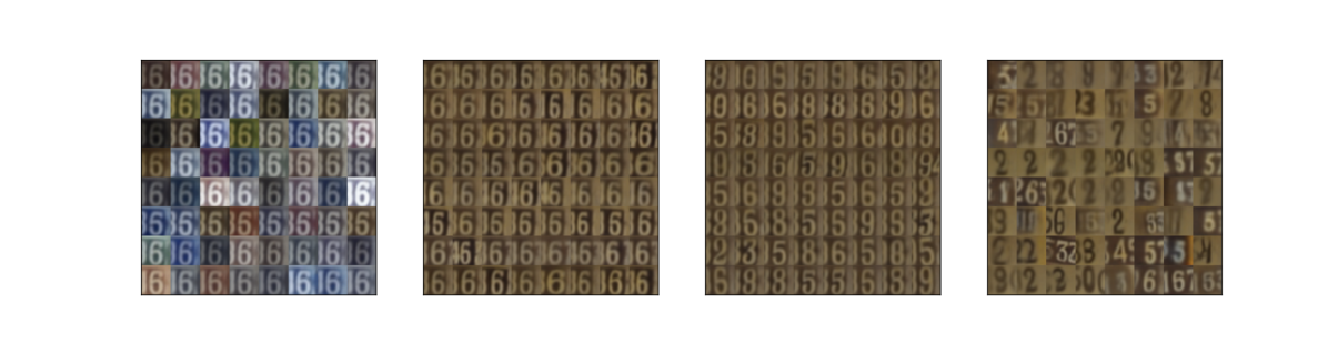
Figure 6: VLAE on SVHN. Each sub-figure corresponds to images generated when fixing latent code on all layers except for one, which we randomly sample from the prior distribution. From left to right the random sampled layer go from bottom layer to top layer. Left panel: The bottom layer represents color schemes; Center-left panel: the second layer represents shape variations of the same digit; Center-right panel: the third layer represents digit identity (interestingly these digits have similar style although having different identities); Right panel: the top layer represents the general structure of the image.

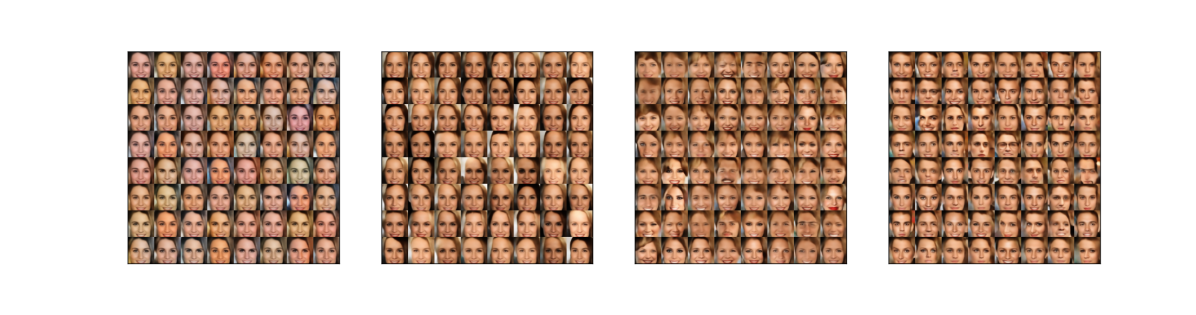
Figure 7: VLAE on CelebA. Each sub-figure corresponds to images generated when fixing latent code on all layers except for one, which we randomly sample from the prior distribution. From left to right the random sampled layer go from bottom layer to top layer. Left panel: The bottom layer represents ambient color; Center-left panel: the second bottom layer represents skin and hair color; Center-right panel: the second top layer represents face identity; Right panel: the top layer presents pose and general structure.

We train VLAE over several datasets and visualize the semantic meaning of the latent code. According to our assumptions, complex, high-level information will be learned by latent codes at higher layers, whereas simple, low-level features will be represented by lower layers.

In Figure 5, we visualize generation results from MNIST, where the model is a 3-layer VLAE with 2 dimensional latent code (${{\bf z}}$) at each layer. The visualizations are generated by systematically exploring the 2D latent code for one layer, while randomly sampling other layers. From the visualization, we see that the three layers encode stroke width, digit width and tilt and digit identity respectively. Remarkably, the semantic meaning of a particular latent code is stable with respect to the sampled latent codes from other layers. For example, in the second layer, the left side represents narrow digits whereas the right side represents wide digits. Sampling latent codes at other layers will control the digit identity, but have no influence over the width. This is interesting given that width is actually correlated with the digit identity; for example, digit 1 is typically thin while digit 0 is mostly wide. Therefore, the model will generate more zeros than ones if the latent code at the second layer corresponds to a wide digit, as displayed in the visualization.

Next we evaluate VLAE on the Street View House Number (SVHN, Netzer et al. (2011)) dataset, where it is significantly more challenging to learn interpretable representations since it is relatively noisy, containing certain digits which do not appear in the center. However, as is shown in Figure 6, our model is able to learn highly disentangled features through a 4-layer ladder, which includes color, digit shape, digit context, and general structure. These features are highly disentangled: since the latent code at the bottom layer controls color, modifying the code from other three layers while keeping the bottom layer fixed will generate a set of image which have the same tone in general. Moreover, the latent code learned at the top layer is the most complex one, which captures rich variations lower layers cannot accurately represent.

Finally, we display compelling results from another challenging dataset, CelebA  (Liu et al., 2015), which includes 200,000 celebrity images. These images are highly varied in terms of environment and facial expressions. We visualize the generation results in Figure 7. As in the SVHN model, the latent code at the bottom layer learns the ambient color of the environment while keeping the personal details intact. Controlling other latent codes will change the other details of the individual, such as skin color, hair color, identity, pose (azimuth); more complicated features are placed at higher levels of the hierarchy.

6 Discussions

Training hierarchical deep generative models is a very challenging task, and there are two main successful families of methods. One family defines the destruction and reconstruction of data using a pre-defined process. Among them, LapGANs (Denton et al., 2015) define the process as repeatedly downsampling, and Diffusion Nets (Sohl-Dickstein et al., 2015) defines a forward Markov chain that coverts a complex data distribution to a simple, tractable one. Without having to perform inference, this makes training much easier, but it does not provide latent variables for other downstream tasks (unsupervised learning).

Another line of work focuses on learning a hierarchy of latent variables by stacking single layer models on top of each other. Many models also use more flexible inference techniques to improve performance  (Sønderby et al., 2016; Dinh et al., 2014; Salimans et al., 2015; Rezende & Mohamed, 2015; Li et al., 2016; Kingma et al., 2016). However we show that there are limitations to stacked VAEs.

Our work distinguishes itself from prior work by explicitly discussing the purpose of learning such models: the advantage of learning a hierarchy is not in better representation efficiency, or better samples, but rather in the introduction of structure in the features, such as hierarchy or disentanglement. This motivates our method, VLAE, which justifies our intuition that a reasonable network structure can be, by itself, highly effective at learning structured (disentangled) representations. Contrary to previous efforts on hierarchical models, we do not stack VAEs on top of each other, instead we use a “flat” approach. This can be applied in combination with the stacking approach.

The results displayed in the experiments resemble those obtained with InfoGAN (Chen et al., 2016); both frameworks learn disentangled representations from the data in an unsupervised manner. The InfoGAN objective, however, explicitly maximizes the mutual information between the latent variables and the observation; whereas in VLAE, this is achieved through the reconstruction error objective which encourages the use of latent codes. Furthermore we are able to explicitly disentangle features with different level of abstractness.

7 Conclusions

In this paper, we discussed the potential practical value of learning a hierarchical generative model over a non-hierarchical one. We show that little can be gained in terms of representation efficiency or sample quality. We further show that traditional HVAE models have trouble learning structured features. Based on these insights, we consider an alternative to learning structured features by leveraging the expressive power of a neural network. Empirical results show that we can learn highly disentangled features.

One limitation of VLAE is the inability to learn structures other than hierarchical disentanglement. Future work should consider more principled ways of designing architectures that allow for learning features with more complex structures.

8 Acknowledgement

This research was supported by Intel Corporation, NSF (#1649208) and Future of Life Institute (#2016-158687).

Appendix A Additional Results

Proposition 2.

$\mathcal{L}_{ELBO}$ for HVAE in Eq.(5) is optimized when $\mathcal{L}_{ELBO}=-H(p_{data}(x))$. If $\mathcal{L}_{ELBO}$ is optimized the following Gibbs sampling chain converges to $p_{data}({{\bf x}})$ if it is ergodic

$${{\bf z}}^{(t)} \sim q({{\bf z}}|{{\bf x}}^{(t)})$$

$${{\bf x}}^{(t+1)} \sim p({{\bf x}}|{{\bf z}}^{(t)})$$ (16)

Proof of Proposition 2.

As in the proof of Proposition 1 when $\mathcal{L}_{ELBO}$ is optimized, $q({{\bf z}}|{{\bf x}})=p({{\bf z}}|{{\bf x}})$. Because the following Gibbs chain converges to $p_{data}({{\bf x}})$

$${{\bf z}}^{(t)} \sim q({{\bf z}}|{{\bf x}}^{(t)})$$

$${{\bf x}}^{(t+1)} \sim q({{\bf x}}|{{\bf z}}^{(t)})$$

We can replace $q({{\bf x}}|{{\bf z}}^{(t)})$ with $p({{\bf x}}|{{\bf z}}^{(t)})$ and the chain still converges to $p_{data}({{\bf x}})$. ∎

Appendix B Experimental Details

B.1 Gaussian HVAE

Architecture: For $l=1,2$

$${{\bf z}}_{l}\sim\mathcal{N}(W_{1}{{\bf f}}_{l}({{\bf z}}_{l+1}),sigm(W_{2}{{\bf f}}_{l}({{\bf z}}_{l+1}))^{2})$$

where $W_{1},W_{2}$ are trainable linear transformation matrices, and $sigm$ is sigmoid activation function. ${{\bf f}}_{l}$ is a two layer dense network. For $l=0$, we let

$${{\bf x}}\sim\mathcal{N}({{\bf f}}_{0}({{\bf z}}_{1}),\sigma^{2}I)$$

where $\sigma$ is a hyper-parameter that can be specified apriori or trained. ${{\bf f}}_{0}$ is a two layer convolutional network with $1/2$ stride for spatial up-sampling. For inference we use the same architecture as the generator.

Learning: During training we use the Adam (Kingma & Ba, 2014) optimizer with learning rate $10^{-4}$. We also anneal the scale the KL-regularization from $0$ to $1$ to encourage use of latent feature during early stages of training.

B.2 VLAE

For VLAE, we use varying layers of convolution depending on size of input image. However, for the ladder connections we do not use convolution. Because of our argument in introduction and Figure 1, generative models do not benefit from convolutional latent features. Therefore we always flatten convolutional layers and apply linear transformation to reduce dimension for each ladder connection. For implementation details please refer to our code.

References

- Bachman (2016) Bachman, Philip. An architecture for deep, hierarchical generative models. In Advances In Neural Information Processing Systems, pp. 4826–4834, 2016.
- Bengio (2009) Bengio, Yoshua. Learning deep architectures for ai. Found. Trends Mach. Learn., 2(1):1–127, January 2009. ISSN 1935-8237. doi: 10.1561/2200000006. URL http://dx.doi.org/10.1561/2200000006.
- Bengio et al. (2009) Bengio, Yoshua et al. Learning deep architectures for ai. Foundations and trends® in Machine Learning, 2(1):1–127, 2009.
- Chen et al. (2016) Chen, X., Duan, Y., Houthooft, R., Schulman, J., Sutskever, I., and Abbeel, P. Infogan: Interpretable representation learning by information maximizing generative adversarial nets. In Advances in Neural Information Processing Systems, pp. 2172–2180, 2016.
- Denton et al. (2015) Denton, E. L., Chintala, S., Fergus, R., et al. Deep generative image models using a laplacian pyramid of adversarial networks. In Advances in neural information processing systems, pp. 1486–1494, 2015.
- Dinh et al. (2014) Dinh, L., Krueger, D., and Bengio, Y. Nice: Non-linear independent components estimation. arXiv preprint arXiv:1410.8516, 2014.
- Donahue et al. (2016) Donahue, Jeff, Krähenbühl, Philipp, and Darrell, Trevor. Adversarial feature learning. arXiv preprint arXiv:1605.09782, 2016.
- Dumoulin et al. (2016) Dumoulin, Vincent, Belghazi, Ishmael, Poole, Ben, Lamb, Alex, Arjovsky, Martin, Mastropietro, Olivier, and Courville, Aaron. Adversarially learned inference. arXiv preprint arXiv:1606.00704, 2016.
- Gulrajani et al. (2016) Gulrajani, Ishaan, Kumar, Kundan, Ahmed, Faruk, Taiga, Adrien Ali, Visin, Francesco, Vázquez, David, and Courville, Aaron C. Pixelvae: A latent variable model for natural images. CoRR, abs/1611.05013, 2016. URL http://arxiv.org/abs/1611.05013.
- Jimenez Rezende et al. (2014) Jimenez Rezende, D., Mohamed, S., and Wierstra, D. Stochastic Backpropagation and Approximate Inference in Deep Generative Models. ArXiv e-prints, January 2014.
- Kaae Sønderby et al. (2016) Kaae Sønderby, C., Raiko, T., Maaløe, L., Kaae Sønderby, S., and Winther, O. Ladder Variational Autoencoders. ArXiv e-prints, February 2016.
- Kingma & Welling (2013) Kingma, D. P and Welling, M. Auto-Encoding Variational Bayes. ArXiv e-prints, December 2013.
- Kingma & Ba (2014) Kingma, Diederik and Ba, Jimmy. Adam: A method for stochastic optimization. arXiv preprint arXiv:1412.6980, 2014.
- Kingma et al. (2016) Kingma, Diederik P, Salimans, Tim, and Welling, Max. Improving variational inference with inverse autoregressive flow. arXiv preprint arXiv:1606.04934, 2016.
- Li et al. (2016) Li, C., Zhu, J., and Zhang, B. Learning to generate with memory. arXiv preprint arXiv:1602.07416, 2016.
- Liu et al. (2015) Liu, Ziwei, Luo, Ping, Wang, Xiaogang, and Tang, Xiaoou. Deep learning face attributes in the wild. In Proceedings of International Conference on Computer Vision (ICCV), 2015.
- Netzer et al. (2011) Netzer, Yuval, Wang, Tao, Coates, Adam, Bissacco, Alessandro, Wu, Bo, and Ng, Andrew Y. Reading digits in natural images with unsupervised feature learning. In NIPS workshop on deep learning and unsupervised feature learning, volume 2011, pp. 5, 2011.
- Pezeshki et al. (2015) Pezeshki, Mohammad, Fan, Linxi, Brakel, Philemon, Courville, Aaron, and Bengio, Yoshua. Deconstructing the ladder network architecture. arXiv preprint arXiv:1511.06430, 2015.
- Radford et al. (2015) Radford, Alec, Metz, Luke, and Chintala, Soumith. Unsupervised representation learning with deep convolutional generative adversarial networks. arXiv preprint arXiv:1511.06434, 2015.
- Rezende & Mohamed (2015) Rezende, D. J. and Mohamed, S. Variational inference with normalizing flows. arXiv preprint arXiv:1505.05770, 2015.
- Salimans et al. (2015) Salimans, T., Kingma, D. P., Welling, M., et al. Markov chain monte carlo and variational inference: Bridging the gap. In International Conference on Machine Learning, pp. 1218–1226, 2015.
- Sohl-Dickstein et al. (2015) Sohl-Dickstein, J., Weiss, E. A., Maheswaranathan, N., and Ganguli, S. Deep unsupervised learning using nonequilibrium thermodynamics. arXiv preprint arXiv:1503.03585, 2015.
- Sønderby et al. (2016) Sønderby, C. K., Raiko, T., Maaløe, L., Sønderby, S. K., and Winther, O. Ladder variational autoencoders. In Advances In Neural Information Processing Systems, pp. 3738–3746, 2016.
- Theis et al. (2015) Theis, Lucas, Oord, Aäron van den, and Bethge, Matthias. A note on the evaluation of generative models. arXiv preprint arXiv:1511.01844, 2015.
- Valpola (2015) Valpola, Harri. From neural pca to deep unsupervised learning. Adv. in Independent Component Analysis and Learning Machines, pp. 143–171, 2015.
- van den Oord et al. (2016) van den Oord, Aaron, Kalchbrenner, Nal, Espeholt, Lasse, Vinyals, Oriol, Graves, Alex, et al. Conditional image generation with pixelcnn decoders. In Advances in Neural Information Processing Systems, pp. 4790–4798, 2016.
- Zeiler & Fergus (2014) Zeiler, Matthew D and Fergus, Rob. Visualizing and understanding convolutional networks. In Computer vision–ECCV 2014, pp. 818–833. Springer, 2014.
- Zhao et al. (2017) Zhao, S., Song, J., and Ermon, S. Towards Deeper Understanding of Variational Autoencoding Models. ArXiv e-prints, February 2017.