Dynamic principle for ensemble control tools

Abstract

Dynamical equations describing physical systems in contact with the thermal bath are commonly extended by mathematical tools called “thermostats”. These tools are designed for sampling ensembles in statistical mechanics. Here we propose a dynamic principle underlying a range of thermostats which is derived using fundamental laws of statistical physics and insures invariance of the canonical measure. The principle covers both stochastic and deterministic thermostat schemes. Our method has a clear advantage over a range of proposed and widely used thermostat schemes which are based on formal mathematical reasoning. Following the derivation of proposed principle we show its generality and illustrate its applications including design of temperature control tools that differ from the Nosé-Hoover-Langevin scheme.

I Introduction

Analysis of molecular systems is an essential part of research in a range of disciplines in natural sciences and in engineering Allen and Tildesley (1989); Frenkel and Smit (2002). As molecular systems affected by environmental thermodynamic conditions, they are studied in the context of statistical physics ensembles. Methods of dynamical sampling of the corresponding probability measures are important for applications and they are under extensive study and development Leimkuhler and Matthews (2015); Tuckerman (2010); Jepps and Rondoni (2010); Bussi et al. (2007); Samoletov et al. (2007); Leimkuhler et al. (2009); Samoletov et al. (2010); Leimkuhler (2010); Bajars et al. (2011); Di Pierro et al. (2015). The traditional application of thermostats is molecular dynamics (MD), that is sampling of equilibrium systems with known potential energy functions, $V(q)$, where $q$ is a system’s configuration. However, the ability to sample equilibrium ensembles at constant temperature $T$ would also imply the ability to sample arbitrary probability measures. Indeed, as an alternative to the conventional MD practice, one may use a probability density $\sigma(q)$, theoretical or extracted from experimental data, to define the potential function as $V(q)=-k_{B}T\,\ln\sigma(q)$, where $k_{B}$ is the Boltzmann constant.

Thermostats embedded into dynamical equations bring in the so-obtained dynamics rich mathematical content. Such dynamical systems with an invariant probability measure have become increasingly popular for mathematical studies in a wide range of applications including investigation of non-equilibrium phenomena Jepps and Rondoni (2010); Dittmar and Kusalik (2014); Ness et al. (2016); Dittmar and Kusalik (2016); Stella et al. (2014); Lepri et al. (1997); Pastorino et al. (2007); Ciccotti and Ferrario (2016), mathematical biology models Bianca (2012); Samoletov and Vasiev (2013); Chow et al. (2005); Tang et al. (2016), multiscale models Mones et al. (2015); Fritz et al. (2011); Praprotnik et al. (2008); Chen et al. (2016); Leimkuhler and Shang (2016), Bayesian statistics and Bayesian machine learning applications Leimkuhler and Shang (2016); Ding et al. (2014); Shang et al. (2015); Noid (2013), superstatistics Fukuda and Moritsugu (2017, 2015).

Here, we present a unified approach for derivation of thermostats sampling the canonical ensemble. The corresponding method is derived using fundamental physical arguments that facilitate understanding physics of thermostat schemes in general, and elucidate physics of the Nosé-Hoover (NH) and the Nosé-Hoover-Langevin (NHL) dynamics in particular. Besides, our method allows to build a plethora of thermostats, stochastic as well as deterministic, including those previously proposed. We expect that it can also be adjusted to arbitrary probability measures.

Classical mechanics and equilibrium statistical physics are adequately described in terms of the Hamiltonian dynamics. Dynamic thermostat schemes involve modified Hamiltonian equations of motion where certain temperature control tools are included. The modified dynamics can be deterministic as well as stochastic Leimkuhler and Matthews (2015); Tuckerman (2010); Samoletov et al. (2007); Leimkuhler et al. (2009); Samoletov et al. (2010); Leimkuhler (2010); Leimkuhler and Matthews (2013); Allen and Tildesley (1989); Hoover (2012); Bussi et al. (2007); Samoletov and Vasiev (2013); Hoover (1985); Nosé (1984); Frenkel and Smit (2002); Bajars et al. (2011); Jepps and Rondoni (2010); Bussi et al. (2009); Di Pierro et al. (2015). Recently proposed NHL thermostats Leimkuhler and Matthews (2015); Samoletov et al. (2007); Leimkuhler et al. (2009); Samoletov et al. (2010) combine deterministic dynamics with stochastic perturbations. This combination ensures ergodicity and allows “gentle” perturbation of the physical dynamics that is often desired Leimkuhler and Matthews (2015); Leimkuhler et al. (2009).

To introduce our scheme, we consider a dynamical system $\mathrm{S}$ consisting of $N$ particles in $d$-dimensional space ($\mathcal{N}=dN$ degrees of freedom) described by the Hamiltonian function $H(x)$, where $x=(p,q)$ is a point in the phase space $\mathcal{M=\mathbb{R}}^{2dN}$, $p=\left\{\mathbf{p}_{i}\in\mathbb{R}^{d}\right\}_{i=1}^{N}$ are momentum variables and $q=\left\{\mathbf{q}_{i}\in\mathbb{R}^{d}\right\}_{i=1}^{N}$ are position variables. The Hamiltonian dynamics has the form, $\dot{x}=\boldsymbol{J}\boldsymbol{\nabla}H(x)$ in the phase space $\mathcal{M}$, where ${\normalcolor\boldsymbol{J}}$ is the symplectic unit. The canonical ensemble describes the system $\mathrm{S}$ in contact with the heat bath $\Sigma$ (an energy reservoir permanently staying in the thermal equilibrium with the thermodynamic temperature $T$), and $\mathrm{S}$ may exchange energy with $\Sigma$ only in the form of heat. Thus, the temperature of the system $\mathrm{S}$ is fixed while its energy, $E$, is allowed to fluctuate. The canonical distribution has the form $\rho_{\infty}(x)\propto\exp\left[-\beta H\left(x\right)\right]$, where $\beta=(k_{B}T)^{-1}$. On average along an ergodic trajectory $\left\langle E(t)\right\rangle=E(T)=const$. Rate of energy exchange between the system $\mathrm{S}$ and the thermal bath $\Sigma$ depends on the temperature $T$. Note that Hamiltonian system is unable to sample the canonical distribution since there is no energy exchange between the system and the heat bath. To describe the heat transfer, it is necessary to modify the equations of motion in a way that the dynamics becomes non-Hamiltonian Ruelle (2004). Suppose $\dot{x}=\boldsymbol{G}(x)$ is a modified law of motion and $\dot{H}(x)=\boldsymbol{G}(x)\cdot\boldsymbol{\nabla}H(x)$ is the rate of energy change (depending on $T$) such that $\left\langle\boldsymbol{G}(x)\cdot\boldsymbol{\nabla}H(x)\right\rangle=0$, that is the energy is constant on average. Let $\boldsymbol{G}(x)\cdot\boldsymbol{\nabla}H(x)\propto F(x,\beta)$ where the temperature dependence is a key. In order to state the dynamic principle governing temperature control tools, a few definitions are required.

II Microscopic temperature expressions

Consider $F(x,\beta)$ such that $\left\langle F(x,\beta)\right\rangle=0$ for all $\beta>0$. This condition is denoted as $F(x,\beta)\sim 0$ while the function $F(x,\beta)$ is called the microscopic temperature expression (TE).

For the system with $H(x)=K(p)+V(q)$ examples of TEs include the kinetic TE, $F_{k\text{in}}(p,\beta)=2K(p)\beta-\mathcal{N}$, and the configurational TE, $F_{conf}(q,\beta)=(\boldsymbol{\nabla}V(q))^{2}\beta-\Delta V(q)$ Rugh (1997).

Various TEs can be obtained in the following manner. Suppose that $F(x,\beta)$ is a polynomial in $\beta$, $F(x,\beta)=\sum_{n=0}^{2L+1}\varphi_{n}(x)\beta^{n}\sim 0$, where $L\in\mathbb{Z}_{\geq 0}$ and functions $\left\{\varphi_{n}(x)\right\}_{n=0}^{2L+1}$, are subject to specification. Rewrite $F(x,\beta)$ in the form

$$F(x,\beta)=\sum_{k=0}^{L}\left(\varphi_{2k}(x)+\beta\varphi_{2k+1}(x)\right)\beta^{2k}\sim 0$$ (1)

for all $\beta>0$. Thus, from (1) it follows that $\varphi_{2k}(x)+\beta\varphi_{2k+1}(x)\sim 0$ for all $k\in\left\{0,1,\ldots,L\right\}$. To find $\varphi_{2k}(x)$ and $\varphi_{2k+1}(x)$ satisfying this condition consider the basic expression, $F(x,\beta)=\beta\,\varphi_{1}(x)+\varphi_{0}(x)$. Substituting $\varphi(x)\partial_{i}H(x)$ for $\varphi_{1}(x)$, where $\varphi(x)$ is an arbitrary function, and utilizing the identity, $\partial_{i}e^{-\beta H(x)}=-\beta\partial_{i}H(x)e^{-\beta H(x)}$ for all $i=1,\ldots,2dN$ and $x\in\mathcal{M}$, where $\partial_{i}\equiv\nicefrac{{\partial}}{{\partial x_{i}}}$, we get $\partial_{i}\varphi(x)+\varphi_{0}(x)\sim 0$. Then, excluding $\varphi_{0}(x)$ from the basic expression, we arrive at $F(x,\beta)=\beta\,\varphi(x)\partial_{i}H(x)-\partial_{i}\varphi(x)\sim 0$ (or $\varphi(x)\partial_{i}H(x)-k_{B}T\partial_{i}\varphi(x)\sim 0$) for each and every $x_{i}$ in $\mathcal{M}$ provided that $\varphi(x)\exp[-\beta H(x)]\rightarrow 0$ as $\left|x\right|\rightarrow\infty$. This result can be represented in a compact form. Suppose $\boldsymbol{\varphi}_{0}(x)$ is a vector field on $\mathcal{M}$ such that $\boldsymbol{\varphi}_{0}(x)\exp[-\beta H(x)]\rightarrow\boldsymbol{0}$ as $\left|x\right|\rightarrow\infty$. Then

$$F_{0}(x,T)=\boldsymbol{\boldsymbol{\varphi}}_{0}(x)\cdot\boldsymbol{\nabla}H(x)-k_{B}T\boldsymbol{\nabla}\cdot\boldsymbol{\varphi}_{0}(x)\sim 0.$$ (2)

This form of TE was previously discussedJepps et al. (2000). More general TEs are allowed, e.g. vector fields $\boldsymbol{F}(x,\beta)=\beta\,\boldsymbol{\nabla}H(x)\times\boldsymbol{\varphi}(x)-\boldsymbol{\nabla}\times\boldsymbol{\varphi}(x)\sim 0$, and so on. As a further generalization we introduce the notation

$$F_{l}(x,T)=\boldsymbol{\boldsymbol{\varphi}}_{l}(x)\cdot\boldsymbol{\nabla}H(x)-k_{B}T\boldsymbol{\nabla}\cdot\boldsymbol{\varphi}_{l}(x),$$

where $l=0,1,...,L$, $\boldsymbol{\boldsymbol{\varphi}}_{0}(x)=\boldsymbol{\boldsymbol{\varphi}}(x)$, and $\left\{\boldsymbol{\boldsymbol{\varphi}}_{l}(x)\right\}_{l=0}^{L}$ is a set of vector fields such that $\boldsymbol{\varphi}_{l}(x)\exp[-\beta H(x)]\rightarrow\boldsymbol{0}$ as $\left|x\right|\rightarrow\infty$. Then the general scalar TE can be represented as

$$F_{L}(x,T)=\sum_{l=0}^{L}F_{l}(x,T)(k_{B}T)^{2l}\sim 0$$ (3)

for all $L\in\mathbb{Z}_{\geq 0}$. A particular example of the use of such a TE in a limited context ($L=1$ and $\boldsymbol{\varphi}_{l}(x)\propto(\boldsymbol{p},0)$ leading to the kinetic TE) can be found in the literatureHoover and Holian (1996). In what follows we focus mainly on $F_{0}(x,T)$ and only to a certain extent on $F_{L}(x,T)$ where $\,L\geq 1$.

Although the expression (2) implies the existence of infinite number of TEs, they all are equivalent from the thermodynamic perspective. However, the time interval required to achieve a specified accuracy in $\left\langle F(x,\beta)\right\rangle=0$ can differ for different TEs Uhlenbeck and Ford (1963). In general, physical systems are often distinguished by multimodal distributions and by existence of metastable states. Their dynamics is characterized by processes occurring on a number of timescales. We assume that TEs can be associated with dynamical processes occurring on various time scales, and thus, they can be combined in multiscale models.

III Dynamic principle

Now we claim the following dynamic principle for ensemble control tools: Let $F(x,T)$ be a TE. Then there exists the dynamical system, $\dot{x}=\boldsymbol{G}(x)$, such that

$$\boldsymbol{\nabla}H(x)\cdot\boldsymbol{G}(x)\propto F(x,T).$$ (4)

Relationship (4) states that the rates of dynamical fluctuations in energy and in TE are proportional, both are zero on average and there is no energy release along a whole trajectory in $\mathcal{M}$. It is a necessary condition for any thermostat. In what follows, with implication of the fundamental requirements of statistical physics, we show that the relationship (4) leads to a general method for obtaining stochastic and deterministic thermostats.

Let us consider the exchange of energy between the system $\mathrm{S}$ and the thermal bath $\Sigma$. Any system placed in the heat bath should in some extent perturb it and be affected by backward influence of this perturbation. There exists a subsystem $\mathrm{S_{ad}}$ of $\Sigma$ such that $\mathrm{S_{ad}}$ is involved in a joint dynamics with $\mathrm{S}$. The rest of the heat bath is assumed to be unperturbed, permanently staying in thermal equilibrium. This is an approximation that is based on separation of relevant time scales. For instance, Brownian dynamics assumes that characteristic time scales of $\mathrm{S}$ and $\Sigma$ are well separated and the system $\mathrm{S}$ does not perturb $\Sigma$. If the time scale is refined (which is of particular importance for small systems) then we have to take into account joint dynamics of $\mathrm{S}$ and $\mathrm{S_{ad}}$. We will show that this case is closely related to NHL Samoletov et al. (2007); Leimkuhler et al. (2009) and NH dynamics Nosé (1984); Hoover (1985).

Thus, we have two cases: (A) the system $\mathrm{S}$ doesn’t perturb the thermal bath and there are no new dynamic variables. The thermal bath in this case can only be taken into account implicitly via stochastic perturbations (similar to the Langevin dynamics); (B) the system $\mathrm{S}$ perturbs a part ($\mathrm{S_{ad}}$) of the thermal bath $\Sigma$, while the rest of the thermal bath remains unperturbed. We assume that there is no direct energy exchange between $\mathrm{S}$ and $\Sigma$. Fundamentals of the statistical mechanics require that the systems $\mathrm{S}$ and $\mathrm{S_{ad}}$ are statistically independent at thermal equilibrium. Let us consider cases A and B in detail.

III.1 Stochastic dynamics

Suppose $\>\boldsymbol{\nabla}H(x)\cdot\dot{x}=\lambda F_{0}(x,T)$, where $\lambda$ is a constant. Without loss of generality, we can consider modified Hamiltonian dynamics in the form, $\dot{x}=\boldsymbol{J}\boldsymbol{\nabla}H(x)+\boldsymbol{\psi}(x,\lambda)$, and consequently:

$$\boldsymbol{\nabla}H(x)\cdot\boldsymbol{\boldsymbol{\psi}}(x,\lambda)=\lambda F_{0}(x,T),$$ (5)

where the vector field $\boldsymbol{\boldsymbol{\psi}}(x,\lambda)$ is to be found. Since the thermal bath does not appear in equation (5) explicitly, only stochastic thermal noise may be involved in the dynamics. To find $\boldsymbol{\boldsymbol{\psi}}$, we introduce $2\mathcal{N}$-vector of independent thermal white noises, $\boldsymbol{\xi}(t)$, such that $\left\langle\boldsymbol{\xi}(t)\right\rangle=\boldsymbol{0}$, $\quad\left\langle\xi_{i}(t)\xi_{j}(t^{\prime})\right\rangle=2\lambda k_{\mathrm{B}}T\delta_{ij}\delta(t-t^{\prime})$, and the vector field, $\boldsymbol{\Phi}(x)$, such that

$$\left\langle\boldsymbol{\xi}(t)\cdot\boldsymbol{\Phi}(x)\right\rangle=\lambda k_{\mathrm{B}}T\,\langle\boldsymbol{\nabla}\cdot\boldsymbol{\varphi}(x)\rangle,$$

where $\left\langle\cdots\right\rangle$ is the Gaussian average over all realizations of $\boldsymbol{\xi}(t)$. Using Novikov’s formula Novikov (1965); Klyatskin (2005), we get

$$\left\langle\boldsymbol{\xi}(t)\cdot\boldsymbol{\Phi}(x)\right\rangle=\,\sum_{i,k}\left\langle\frac{\partial\Phi_{k}}{\partial x_{i}}\frac{\delta x_{i}(t)}{\delta\xi_{k}(t)}\right\rangle\lambda k_{\mathrm{B}}T.$$

Suppose $\frac{\delta x_{i}(t)}{\delta\xi_{k}(t)}=\zeta_{i}(x)\delta_{ik}$, where the vector field $\boldsymbol{\zeta}(x)$ is such that each component $\zeta_{i}(x)$ does not depend on $x_{i}$, that is

$$\boldsymbol{\nabla}\circ\boldsymbol{\zeta}(x)=\boldsymbol{0},$$

where $\circ$ denotes the component-wise (Hadamard) product of two vectors and $\boldsymbol{0}$ is the null vector. Then $\boldsymbol{\nabla}\cdot\boldsymbol{\varphi}(x)=\boldsymbol{\nabla}\cdot(\boldsymbol{\zeta}(x)\circ\boldsymbol{\Phi}(x))$. Thus, we get $\boldsymbol{\varphi}(x)=\boldsymbol{\zeta}(x)\circ\boldsymbol{\Phi}(x)$ and it follows that $\boldsymbol{\Phi}(x)=\boldsymbol{\zeta}^{-1}(x)\circ\boldsymbol{\varphi}(x)$, where $\boldsymbol{\zeta}^{-1}(x)$ is the vector field such that $\boldsymbol{\zeta}^{-1}(x)\circ\boldsymbol{\zeta}(x)=\boldsymbol{1}$. Assuming $\boldsymbol{\varphi}(x)=\boldsymbol{\eta}(x)\circ\boldsymbol{\nabla}H(x)$, where $\boldsymbol{\eta}(x)\equiv\boldsymbol{\zeta}(x)\circ\boldsymbol{\zeta}(x)$, we get

$$\boldsymbol{\psi}(x,\lambda)=-\lambda\boldsymbol{\eta}(x)\circ\boldsymbol{\nabla}H(x)+\boldsymbol{\zeta}(x)\circ\boldsymbol{\xi}(t)$$

and the modified Hamiltonian dynamics takes the form of stochastic differential equation (SDE):

$$\dot{x}=\boldsymbol{J}\boldsymbol{\nabla}H(x)-\lambda\boldsymbol{\eta}(x)\circ\boldsymbol{\nabla}H(x)+\boldsymbol{\zeta}(x)\circ\boldsymbol{\xi}(t).$$ (6)

The Fokker-Planck equation (FPE) corresponding to SDE (6) has the form $\partial_{t}\rho=\boldsymbol{\mathcal{F}}^{*}\rho$, where

$$\boldsymbol{\mathcal{F}}^{*}\rho=-\boldsymbol{J}\boldsymbol{\nabla}H(x)\cdot\boldsymbol{\boldsymbol{\nabla}}\rho+\lambda\boldsymbol{\boldsymbol{\nabla}}\cdot[\boldsymbol{\eta}(x)\circ\boldsymbol{\nabla}H(x)\,\rho]$$

$$+\lambda k_{B}T\!\boldsymbol{\nabla\cdot}[\boldsymbol{\eta}(x)\circ\boldsymbol{\nabla}\rho].$$

Note that the last term here was found using the following specific relationship for the vector field $\boldsymbol{\zeta}(x)$:

$$\left(\boldsymbol{\zeta}(x)\circ\boldsymbol{\nabla}\right)\cdot\left(\boldsymbol{\zeta}(x)\circ\boldsymbol{\nabla}\rho\right)=\boldsymbol{\nabla\cdot}[\boldsymbol{\eta}(x)\circ\boldsymbol{\nabla}\rho].$$

Invariant probability density for dynamics (6) is determined by the equation $\boldsymbol{\mathcal{F}}^{*}\rho=0$. It is expected that this is a unique invariant density Mattingly et al. (2002); Leimkuhler et al. (2009).

We claim that for the defined above vector field $\boldsymbol{\zeta}(y)$ the canonical density, $\rho_{\infty}\propto\exp\left[-\beta H\left(x\right)\right]$, is invariant for the stochastic dynamics given by (6), that is $\boldsymbol{\mathcal{F}}^{*}\rho_{\infty}=0$. The proof is by direct calculation.

The Langevin equation is a particular case of (6). For example, for the system with $H(x)=\nicefrac{{p^{2}}}{{2m}}+V(q)$, where $x=(p,q)\in\mathbb{R}^{2}$ we have:

• if $\boldsymbol{\zeta}=(1,0)$, then
  $\dot{p}=-V^{\prime}(q)-\lambda\nicefrac{{p}}{{m}}+\xi(t)$, $\dot{q}=\nicefrac{{p}}{{m}}$;

• if $\boldsymbol{\zeta}=(0,1)$, then
  $\dot{p}=-V^{\prime}(q)$, $\dot{q}=\nicefrac{{p}}{{m}}-\lambda V^{\prime}(q)+\xi(t)$.

The procedure for obtaining stochastic dynamics (6) is essentially a general and can be a quite straightforwardly extended to other TEs, for example, the general scalar TE (3). Indeed, let us introduce the set of $2\mathcal{N}$-vectors of independent thermal white noises, $\left\{\boldsymbol{\xi}(l;t)\right\}_{l=0}^{L},\,L\in\mathbb{Z}_{\geq 0}$, such that $\left\langle\boldsymbol{\xi}(l;t)\right\rangle=\boldsymbol{0}$, $\quad\left\langle\xi_{i}(l;t)\xi_{j}(l^{\prime};t^{\prime})\right\rangle=2\lambda_{l}k_{\mathrm{B}}T\delta_{ij}\delta_{ll^{\prime}}\delta(t-t^{\prime})$, and the set of vector fields, $\left\{\boldsymbol{\zeta}(l;x)\right\}_{l=0}^{L},\,L\in\mathbb{Z}_{\geq 0}$, such that $\boldsymbol{\nabla}\circ\boldsymbol{\zeta}(l;x)=\boldsymbol{0}$ for any $l\geq 0$, where $\circ$ denotes the component-wise (Hadamard) product of two vectors and $\boldsymbol{0}$ is the null vector. Starting from the relationship,

$$\boldsymbol{\nabla}H(x)\cdot\boldsymbol{\boldsymbol{\psi}}(x,\lambda)=\sum_{l=0}^{L}\lambda_{l}F_{l}(x,T)\,(k_{B}T)^{2l},$$

and then strictly following arguments as stated above, we get

$$\boldsymbol{\psi}(x,\lambda)=-\sum_{l=0}^{L}\lambda_{l}\boldsymbol{\eta}(l;x)\circ\boldsymbol{\nabla}H(x)\,(k_{B}T)^{2l}\\ +\sum_{l=0}^{L}\boldsymbol{\zeta}(l;x)\circ\boldsymbol{\xi}(l;t)\,(k_{B}T)^{l}.$$

where $\boldsymbol{\eta}(x)\equiv\boldsymbol{\zeta}(x)\circ\boldsymbol{\zeta}(x)$. Thus, we arrive at the following stochastic dynamics

$$\dot{x}=\boldsymbol{J}\boldsymbol{\nabla}H(x)-\sum_{l=0}^{L}\lambda_{l}\boldsymbol{\eta}(l;x)\circ\boldsymbol{\nabla}H(x)\,(k_{B}T)^{2l}\\ +\sum_{l=0}^{L}\boldsymbol{\zeta}(l;x)\circ\boldsymbol{\xi}(l;t)\,(k_{B}T)^{l}.$$ (7)

One can verify that the canonical measure is invariant for this stochastic equation of motion. Generally speaking, the dynamics (7) includes $2\mathcal{N}(L+1)$ independent white noise processes. This seems impractical. However, we can point out that (7) potentially useful for multi-timescale stochastic simulations. As a simple example, let $H(x)=\nicefrac{{p^{2}}}{{2m}}+V(q)$, $L=1$, $\boldsymbol{\zeta}(0;x)=(1,0)$, and $\boldsymbol{\zeta}(1;x)=(0,1)$, then we arrive at the stochastic dynamics with two timescales involved,

$$\dot{p}=-V^{\prime}(q)-\lambda_{0}\frac{p}{m}+\xi_{p}(0;t),$$

$$\dot{q}=\frac{p}{m}-\lambda_{1}\left(k_{B}T\right)^{2}\,V^{\prime}(q)+k_{B}T\,\xi_{q}(1;t),$$

where $\left\langle\xi_{p}(0;t)\right\rangle=0,\,\left\langle\xi_{q}(1;t)\right\rangle=0$, $\left\langle\xi_{p}(0;t)\xi_{q}(1;t)\right\rangle=0$, $\left\langle\xi_{p}(0;t)\xi_{p}(0;t^{\prime})\right\rangle=2\lambda_{0}k_{\mathrm{B}}T\delta(t-t^{\prime})$, $\left\langle\xi_{q}(1;t)\xi_{q}(1;t^{\prime})\right\rangle=2\lambda_{1}k_{\mathrm{B}}T\delta(t-t^{\prime})$, as specified above. Analysis of $p-$ and $q-$dynamics can be performed in reduced systems following the separation of these variables according to their time scales Samoletov (1999).

III.2 Deterministic and stochastic dynamics

Let $\mathrm{S_{ad}}$ be associated with an even-dimensional phase space $\mathcal{M}_{\mathrm{ad}}$, the Hamiltonian function $h(y)$, $y\in\mathcal{M}_{\mathrm{ad}}$, and the Hamiltonian dynamics, $\dot{y}=\boldsymbol{J}_{y}\boldsymbol{\nabla}_{y}h(y)$, where $\boldsymbol{J}_{y}$ is the symplectic unit. Without loss of generality, we can assume that the modified Hamiltonian dynamics of the system composed by $\mathrm{S}$ and $\mathrm{S_{ad}}$ has the form,

$$\dot{x}=\boldsymbol{J}_{x}\boldsymbol{\nabla}_{x}H(x)+\boldsymbol{\psi}(x,y),$$

$$\dot{y}=\boldsymbol{J}_{y}\boldsymbol{\nabla}_{y}h(y)+\boldsymbol{\psi}^{\ast}(y,x),$$

where $\boldsymbol{\psi}(x,y)$ and $\boldsymbol{\psi}^{*}(y,x)$ are vector fields on $\mathcal{M}$ and $\mathcal{M}_{\mathrm{ad}}$ correspondingly. To derive deterministic dynamics, let us temporarily ignore the heat exchange between $\mathrm{S_{ad}}$ and $\Sigma$, that is, $\boldsymbol{\nabla}_{y}h(y)\cdot\boldsymbol{\psi}^{\ast}(y,x)=\lambda^{\ast}{F}^{\ast}(y,T)$ and $\boldsymbol{\nabla}_{x}H(x)\cdot\boldsymbol{\psi}(x,y)=\lambda{F}(x,T)$. As discussed above, these relationships lead to the stochastic dynamics. Systems $\mathrm{S}$ and $\mathrm{S_{ad}}$ must be statistically independent in the thermal equilibrium, so that $\boldsymbol{\nabla}_{x}H(x)\cdot\dot{x}\sim 0$ and $\boldsymbol{\nabla}_{y}h(y)\cdot\dot{y}\sim 0$ are satisfied simultaneously. Thus, we assume that

$$\boldsymbol{\nabla}_{x}H(x)\cdot\boldsymbol{\psi}(x,y) =g(x)F_{0}^{\ast}(y,T),$$

$$\boldsymbol{\nabla}_{y}h(y)\cdot\boldsymbol{\psi}^{\ast}(y,x) =-g^{\ast}(y)F_{0}(x,T),$$

where $g(x)$ and $g^{\ast}(y)$ are some vague functions, and

$$F_{0}(x,T)=\boldsymbol{\boldsymbol{\varphi}}(x)\cdot\boldsymbol{\nabla}_{x}H(x)-k_{B}T\,\boldsymbol{\nabla}_{x}\cdot\boldsymbol{\varphi}(x),$$

$$F_{0}^{\ast}(y,T)=\boldsymbol{Q}(y)\cdot\boldsymbol{\nabla}_{y}h(y)-k_{B}T\,\boldsymbol{\nabla}_{y}\cdot\boldsymbol{Q}(y),$$ (8)

are TEs for the systems $\mathrm{S}$ and $\mathrm{S_{ad}}$ correspondingly. These relationships are valid for any $H(x)$ and $h(y)$. To specify $\boldsymbol{\psi}(x,y)$ and $\boldsymbol{\psi}^{*}(y,x)$, we assume that $g(x)=\boldsymbol{\boldsymbol{a}}(x)\cdot\boldsymbol{\nabla}_{x}H(x)$, $g^{\ast}(y)=\boldsymbol{b}(y)\cdot\boldsymbol{\nabla}_{y}h(y)$, where $\boldsymbol{a}(x)$ and $\boldsymbol{b}(y)$ are vector fields on $\mathcal{M}$ and $\mathcal{M}_{\mathrm{ad}}$, respectively. It follows that

$$\boldsymbol{\psi}(x,y)=\boldsymbol{\boldsymbol{a}}(x)\,F_{0}^{\ast}(y,T),\quad\boldsymbol{\psi^{\ast}}(y,x)=\boldsymbol{b}(y)\,F_{0}(x,T).$$

To determine the relationship between the vector fields $\boldsymbol{a}(x)$, $\boldsymbol{b}(y)$ and TEs $F_{0}(x,T)$, $F_{0}^{\ast}(y,T)$, recall that if the combined system $\mathrm{S+S_{ad}}$ is isolated, then $\dot{H}(x)=-\dot{h}(y)$; and if $T\neq 0$, then $\dot{H}(x)+\dot{h}(y)\sim 0$. Straightforward calculations show that

$$\boldsymbol{a}(x)=\boldsymbol{\varphi}(x),\quad\boldsymbol{b}(y)=\boldsymbol{Q}(y),$$

provided that $\boldsymbol{b}(y)\exp[-\beta h(y)]\underset{}{\rightarrow}\boldsymbol{0}$ as $\left|y\right|\rightarrow\infty$ and $\boldsymbol{a}(x)\exp[-\beta H(x)]\rightarrow\boldsymbol{0}$ as $\left|x\right|\rightarrow\infty$. As a result, we have the equations of motion

$$\dot{x}=J_{x}\mathbb{\boldsymbol{\nabla}}_{x}H(x)+F_{0}^{\ast}(y,T)\boldsymbol{\boldsymbol{\varphi}}(x),$$ (9)

$$\dot{y}=\boldsymbol{J}_{y}\boldsymbol{\nabla}_{y}h(y)-F_{0}(x,T)\boldsymbol{Q}(y),$$

which are generalized NH equations.

The Liouville equation associated with the system (9) has the form $\partial_{t}\rho=-\mathcal{L}^{*}\rho$, where $\mathcal{L}^{*}\rho=\boldsymbol{\nabla}_{x}\cdot(\dot{x}\rho)+\boldsymbol{\nabla}_{y}\cdot(\dot{y}\rho)$. Invariant probability densities are determined by the equation $\mathcal{L}^{*}\rho=0$. We claim that if $\boldsymbol{Q}(y)$ and $\boldsymbol{\varphi}(x)$ are the defined above vector fields, then the canonical density $\rho_{\infty}\propto\exp\left[-\beta H\left(x\right)\right]\cdot\exp\left[-\beta h\left(y\right)\right]$ is invariant for dynamics (9), that is $\mathcal{L}^{*}\rho_{\infty}=0$. The proof is by direct calculation.

As a particular case, let $\boldsymbol{Q}(y)$ be an incompressible vector field (i.e. $\boldsymbol{\nabla}_{y}\cdot\boldsymbol{Q}(y)=0$ for all $y\in\mathcal{M}_{\mathrm{ad}}$). Then we arrive at the NH equations

$$\dot{x}=J_{x}\mathbb{\boldsymbol{\nabla}}_{x}H(x)+\left(\boldsymbol{Q}(y)\cdot\boldsymbol{\nabla}_{y}h(y)\right)\boldsymbol{\boldsymbol{\varphi}}(x),$$ (10)

$$\dot{y}=\boldsymbol{J}_{y}\boldsymbol{\nabla}_{y}h(y)-F_{0}(x,T)\boldsymbol{Q}(y).$$

Now we include into our consideration the effect of the thermal bath $\Sigma$ on $\mathrm{S_{ad}}$ dynamics, that is the relationship $\boldsymbol{\nabla}_{y}h(y)\cdot\boldsymbol{\psi}^{\ast}=\lambda F_{0}^{\ast}(y,T)$. Following the arguments and notations used to derive SDE (6), we arrive at the stochastic dynamics:

$$\dot{x}=\boldsymbol{J}_{x}\mathbb{\boldsymbol{\nabla}}_{x}H(x)+F_{0}^{\ast}(y,T)\,\boldsymbol{\varphi}(x),$$

$$\dot{y}=\boldsymbol{J}_{y}\boldsymbol{\nabla}_{y}h(y)-F_{0}(x,T)\,\boldsymbol{Q}(y)-\lambda\boldsymbol{\eta}(y)\circ\boldsymbol{\nabla}_{y}h(y)$$

$$+\boldsymbol{\zeta}(y)\circ\boldsymbol{\xi}(t),$$ (11)

which are generalized NHL equationsSamoletov et al. (2007); Leimkuhler et al. (2009). In the particular case of an incompressible vector field $\boldsymbol{Q}(y)$ we get the NHL equations:

$$\dot{x}=\boldsymbol{J}_{x}\mathbb{\boldsymbol{\nabla}}_{x}H(x)+\left(\boldsymbol{Q}(y)\cdot\boldsymbol{\nabla}_{y}h(y)\right)\,\boldsymbol{\varphi}(x),$$

$$\dot{y}=\boldsymbol{J}_{y}\boldsymbol{\nabla}_{y}h(y)-F_{0}(x,T)\,\boldsymbol{Q}(y)-\lambda\boldsymbol{\eta}(y)\circ\boldsymbol{\nabla}_{y}h(y)$$

$$+\boldsymbol{\zeta}(y)\circ\boldsymbol{\xi}(t),$$ (12)

FPE corresponding to (11) has the form $\partial_{t}\rho=\mathcal{F}^{*}\rho$, where

$$\boldsymbol{\mathcal{F}}^{*}\rho=-\boldsymbol{J}_{x}\boldsymbol{\nabla}_{x}H(x)\cdot\boldsymbol{\boldsymbol{\nabla}}_{x}\rho-\boldsymbol{J}_{y}\boldsymbol{\nabla}_{y}h(y)\cdot\boldsymbol{\nabla}_{y}\rho$$

$$-F_{0}^{\ast}(y,T)\boldsymbol{\nabla}_{x}\cdot\left[\boldsymbol{\varphi}(x)\rho\right]+F_{0}(x,T)\boldsymbol{\nabla}_{y}\cdot\left[\boldsymbol{Q}(y)\rho\right]$$

$$+\lambda k_{B}T\boldsymbol{\nabla}_{y}\cdot[\boldsymbol{\eta}(y)\circ\boldsymbol{\nabla}_{y}\rho]+\lambda\boldsymbol{\boldsymbol{\nabla}}_{y}\cdot[\boldsymbol{\eta}(y)\circ\boldsymbol{\nabla}_{y}h(y)\rho].$$

Invariant probability density for the SDE (11) is determined by the equation $\mathcal{F}^{*}\rho=0$.

We claim that if $\boldsymbol{Q}(y)$, $\boldsymbol{\varphi}(x)$, and $\boldsymbol{\zeta}(y)$ are the defined above vector fields , then the canonical density, $\rho_{\infty}\propto\exp\left[-\beta H\left(x\right)\right]\cdot\exp\left[-\beta h\left(y\right)\right]$, is invariant for the NHL dynamics (11), that is $\mathcal{F}^{*}\rho_{\infty}=0$. The proof is by direct calculation.

Besides, we expect that this dynamics is ergodic Mattingly et al. (2002); Leimkuhler et al. (2009).

Commonly used NH Nosé (1984); Hoover (1985) and NHL Samoletov et al. (2007); Leimkuhler et al. (2009); Samoletov et al. (2010) thermostats are particular cases of thermostats given by (10) and (12) correspondingly. For example, by substituting $\nicefrac{{\zeta^{2}}}{{2Q}}$ for $h(y),\,y=(\zeta,\eta)\in\mathbb{R}^{2}$, $(-Q,0)$ for $\boldsymbol{Q}(y)$ and $(\mathbf{p},0)$ for $\boldsymbol{\varphi}(x)$ in (9) we get classical NH equations Nosé (1984); Hoover (1985).

It is worth to note that the case of the general TE can be considered straightforwardly following the method of dynamic principle, as developed above. Assume that

$$\boldsymbol{\nabla}_{x}H(x)\cdot\boldsymbol{\psi}(x,y) =\sum_{l=0}^{L}g_{l}(x)F_{l}^{\ast}(y,T)\,(k_{B}T)^{2l},$$

$$\boldsymbol{\nabla}_{y}h(y)\cdot\boldsymbol{\psi}^{\ast}(y,x) =-\sum_{l=0}^{L}g_{l}^{\ast}(y)F_{l}(x,T)\,(k_{B}T)^{2l}.$$

These relationships must be valid for any $H(x)$ and $h(y)$. To specify $\boldsymbol{\psi}(x,y)$ and $\boldsymbol{\psi}^{*}(y,x)$, we set $g_{l}(x)=\boldsymbol{\boldsymbol{a}}_{l}(x)\cdot\boldsymbol{\nabla}_{x}H(x)$, $g_{l}^{\ast}(y)=\boldsymbol{b}_{l}(y)\cdot\boldsymbol{\nabla}_{y}h(y)$, from what follows that $\boldsymbol{a}_{l}(x)=\boldsymbol{\boldsymbol{\varphi}}_{l}(x)$ and $\boldsymbol{b}_{l}(y)=\boldsymbol{Q}_{l}(y)$. Thus,

$$\boldsymbol{\psi}(x,y)=\sum_{l=0}^{L}F_{l}^{\ast}(y,T)\,(k_{B}T)^{2l}\boldsymbol{\boldsymbol{\varphi}}_{l}(x),$$

$$\boldsymbol{\psi}^{\ast}(y,x)=-\sum_{l=0}^{L}F_{l}(x,T)\,(k_{B}T)^{2l}\boldsymbol{Q}_{l}(y).$$

Finally, we arrive at the deterministic equations of motion (modified Hamiltonian dynamics),

$$\dot{x}= J_{x}\mathbb{\boldsymbol{\nabla}}_{x}H(x)+\sum_{l=0}^{L}F_{l}^{\ast}(y,T)\,(k_{B}T)^{2l}\boldsymbol{\boldsymbol{\varphi}}_{l}(x),$$

$$\dot{y}= \boldsymbol{J}_{y}\boldsymbol{\nabla}_{y}h(y)-\sum_{l=0}^{L}F_{l}(x,T)\,(k_{B}T)^{2l}\boldsymbol{Q}_{l}(y).$$ (13)

We will not discuss the equations (13) in detail and only note that the canonical measure is invariant for this dynamics, and a generalization to stochastic NHL type dynamics can be obtained. Strictly speaking, such a generalization is important since it simulates an equilibrium reservoir of the energy and ensures the ergodicity of dynamics. To outline a connection between equations of motion (13) and known deterministic thermostatsHoover and Holian (1996); Hoover et al. (2015, 2016); Patra and Bhattacharya (2014, 2015), we provide the following simple example. Let $L=1$, $H(x)=\nicefrac{{p^{2}}}{{2m}}+V(q)$, $h(y)=\nicefrac{{\eta_{0}^{2}}}{{2Q_{0}}}+\nicefrac{{\eta_{1}^{2}}}{{2Q_{1}}}$, $\boldsymbol{\varphi}_{0}(x)=(p,0)$, $\boldsymbol{\varphi}_{1}(x)=(p^{3},0)$, $\boldsymbol{Q}_{0}(y)=(-Q_{0},0,0,0)$, and $\boldsymbol{Q}_{1}(y)=(0,-Q_{1},0,0)$, then

$$\dot{p}=-V^{\prime}(q)-\eta_{0}p-\eta_{1}k_{B}T\,p^{3},$$

$$\dot{q}=\frac{p}{m},$$

$$\dot{\eta}_{0}=Q_{0}\left(\frac{p^{2}}{m}-k_{B}T\right),$$

$$\dot{\eta}_{1}=Q_{1}\left(\frac{p^{4}}{m}-3k_{B}Tp^{2}\right)(k_{B}T)^{2},$$

the dynamic equations equipped with the control of first two moments of the equilibrium kinetic energyHoover and Holian (1996); Hoover et al. (2016). Similarly, we can obtain dynamic equations that control the configurational temperature moments.

IV Redesign of NHL thermostat

In this Section we consider an alternative to the conventional NH and NHL thermostat schemes. This alternative (seen as a particular case of dynamical equations (11)) is based on the consideration of physically reasonable chain of interactions, $\mathrm{S\leftrightsquigarrow S_{ad}}\leftrightsquigarrow\Sigma$, that is, the system $\mathrm{S_{ad}}$ is a buffer between the physical system $\mathrm{S}$ and the infinite energy reservoir $\mathrm{\Sigma}$.

Consider the dynamical equations (9) and (11), and assume that $\boldsymbol{\nabla}_{x}\cdot\boldsymbol{\boldsymbol{\varphi}}(x)=0,\>\boldsymbol{\nabla}_{y}\cdot\boldsymbol{Q}(y)\neq 0$. Note, that these assumptions are opposite to the requirements for the NH and NHL dynamics, where $\boldsymbol{\nabla}_{x}\cdot\boldsymbol{\boldsymbol{\varphi}}(x)\neq 0,\>\boldsymbol{\nabla}_{y}\cdot\boldsymbol{Q}(y)=0$. We get

$$\dot{x} =\boldsymbol{J}_{x}\mathbb{\boldsymbol{\nabla}}_{x}H(x)$$

$$+\left[\boldsymbol{Q}(y)\cdot\boldsymbol{\nabla}_{y}h(y)-k_{B}T\,\boldsymbol{\nabla}_{y}\cdot\boldsymbol{Q}(y)\right]\,\boldsymbol{\varphi}(x),$$

$$\dot{y} =\boldsymbol{J}_{y}\boldsymbol{\nabla}_{y}h(y)-\left(\boldsymbol{\boldsymbol{\varphi}}(x)\cdot\boldsymbol{\nabla}_{x}H(x)\right)\boldsymbol{Q}(y),$$ (14)

and

$$\dot{x} =\boldsymbol{J}_{x}\mathbb{\boldsymbol{\nabla}}_{x}H(x)$$

$$+\left[\boldsymbol{Q}(y)\cdot\boldsymbol{\nabla}_{y}h(y)-k_{B}T\,\boldsymbol{\nabla}_{y}\cdot\boldsymbol{Q}(y)\right]\,\boldsymbol{\varphi}(x),$$

$$\dot{y} =\boldsymbol{J}_{y}\boldsymbol{\nabla}_{y}h(y)-\left(\boldsymbol{\boldsymbol{\varphi}}(x)\cdot\boldsymbol{\nabla}_{x}H(x)\right)\,\boldsymbol{Q}(y)$$

$$-\lambda\boldsymbol{\eta}(y)\circ\boldsymbol{\nabla}_{y}h(y)+\boldsymbol{\zeta}(y)\circ\boldsymbol{\xi}(t),$$ (15)

where vector fields involved are such as indicated above. Thus, there is plenty of freedom in specification of particular thermostat equations of motion.

To illustrate the redesigned NH and NHL thermostat dynamical systems (described by the equations (14) and (15) correspondingly) let us consider system $\mathrm{S}$ with the Hamiltonian function $H\left(p,q\right)$,

$$H\left(p,q\right)=\frac{p^{2}}{2m}+\frac{1}{2}m\omega^{2}q^{2},\quad x=(p,q)\in\mathbb{R}\times\mathbb{R},$$

that is a harmonic oscillator of mass $m$ and frequency $\omega$, and system $\mathrm{S_{ad}}$ with the Hamiltonian function $h(v,u)$,

$$h(v,u)=\frac{v^{2}}{2\mu},\quad y=(v,u)\in\mathbb{R}\times\mathbb{R},$$

that is a free particle of mass $\mu$. Harmonic oscillators are among central instruments in analysis of many physical problems, classical as well as quantum mechanical. It is known that generating the canonical statistics for a harmonic oscillator is a hard problem. For example, the NH scheme is proven to be non-ergodicLegoll et al. (2007) and the NHL schemeSamoletov et al. (2007); Leimkuhler et al. (2009), and earlier the NHC schemeMartyna et al. (1992), was proposed to overcome this difficulty. Anyway, it is important for any dynamic thermostat to correctly generate the canonical statistics for a harmonic oscillator.

The deterministic thermostat dynamics (14) as well as stochastic dynamics (15) allow a plethora of further specifications. To be as close as possible to redesign of original NH dynamicsHoover (1985), we set $\boldsymbol{Q}(y)=(v,0)$, $\boldsymbol{\nabla}\cdot\boldsymbol{Q}=1$, and $\boldsymbol{\varphi}(x)=(\gamma,0)$, where $\gamma$ is a dimensional parameter, $\boldsymbol{\nabla}\cdot\boldsymbol{\boldsymbol{\varphi}}=0$. Thus, we arrive at the following equations of motion:

$$\dot{p} =-m\omega^{2}q+\gamma\left[\frac{v^{2}}{\mu}-k_{B}T\right],$$

$$\dot{q} =\frac{1}{m}p,$$

$$\dot{v} =-\gamma\frac{p}{m}v,$$

$$\dot{u} =\frac{v}{\mu};$$ (16)

and

$$\dot{p} =-m\omega^{2}q+\gamma\left[\frac{v^{2}}{\mu}-k_{B}T\right],$$

$$\dot{q} =\frac{1}{m}p,$$

$$\dot{v} =-\gamma\frac{p}{m}v-\lambda\frac{v}{\mu}+\xi(t),$$

$$\dot{u} =\frac{v}{\mu};$$ (17)

where $\boldsymbol{\zeta}=(1,0)$ and $\left\langle\xi(t)\xi(t^{\prime})\right\rangle=2\lambda k_{\mathrm{B}}T\delta(t-t^{\prime})$. Note, that equations (16) and (17) are redesign of NH (denote RNH) and NHL (RNHL) thermostats correspondingly.

System (16) has two integrals of motion, that is

$$I_{1}=v\exp\left(\gamma q\right)=\mathrm{const},$$

$$I_{2}=\frac{p^{2}}{2m}+\frac{1}{2}m\omega^{2}q^{2}+\frac{v^{2}}{2\mu}+\frac{\gamma k_{B}T}{m}q=\mathrm{const},$$

indicating the lack of ergodicity. For example, if all parameters of the system (16) are set equal to unity, $m=1,\omega=1,\mu=1,\gamma=1,k_{B}T=1$, and initial conditions are $p=1,q=0,v=1$, then the phase trajectory is represented by the closed curve and the Poincaré section (p,q) shown on Figure 1. This is expected from the existence of two integrals of motion, that is $I_{1}$ and $I_{2}$. It is clear that the trajectory does not explore the phase space available for the harmonic oscillator. This ergodicity problem is not surprising, the convenient NH dynamic suffer from the same problem. It is questionable that the situation can be improved with a more complex $\boldsymbol{\varphi}$ and $\boldsymbol{Q}$, for example, $\boldsymbol{\varphi}=(\gamma_{1},\gamma_{2})$, $\boldsymbol{\varphi}=\left(\gamma_{1}m\omega^{2}q,\gamma_{2}\tfrac{1}{m}p\right)$, $\boldsymbol{Q}=(v,u)$, and so on. If $\boldsymbol{\varphi}=(\gamma_{1},\gamma_{2})$, then we get

$$\dot{p} =-m\omega^{2}q+\gamma_{1}\left[\frac{v^{2}}{\mu}-k_{B}T\right],$$

$$\dot{q} =\frac{p}{m}+\gamma_{2}\left[\frac{v^{2}}{\mu}-k_{B}T\right],$$

$$\dot{v} =-\left(\gamma_{1}\frac{p}{m}+\gamma_{2}\mu\omega^{2}q\right)v,$$

$$\dot{u} =\frac{v}{\mu},$$

and it is easy to show that this dynamics is not ergodic.

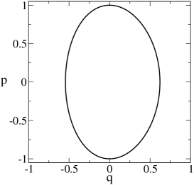
Figure 1: The Poincaré section (p,q) for deterministic dynamic thermostat (16) where all system parameters are set equal to unity and initial condition are: $p=1,q=0,v=1$.

Our next illustration will be devoted to the system described by thermostat dynamical equations (17). We will show, by means of numerical simulations, that a certain realization of the whole length chain of physically reasonable interactions, that is $\mathrm{S\leftrightsquigarrow S_{ad}}\leftrightsquigarrow\Sigma$, generates the correct statistics.

Let us consider the case when all parameters of the system (17) are set equal to unity, $m=1,\omega=1,\mu=1,\gamma=1,k_{B}T=1,\lambda=1$, and the initial conditions are: $p=0,q=0,v=0$. Phase trajectories of length $10^{6}$ are generated using the Euler method with a time step of $\Delta t=0.0005$. We have repeated simulations using the fourth-order Runge-Kutta method with a random contribution held once for the entire interval from $t$ to $t+\Delta t$, and arrive at the same result.

Figure 2(a) shows the Poincaré section (p,q) for a harmonic oscillator equipped with the temperature control tool (17). This figure demonstrates that the trajectory generates proper sampling of the full phase space of the harmonic oscillator. Figures 2(b) and 2(c) show the momentum and position distribution functions from simulations as compared with the exact analytical expressions. In both cases, the Gaussian distribution is generated in agreement with the theoretical prediction. Presented results serve as an evidence of ergodic sampling the canonical statistics.

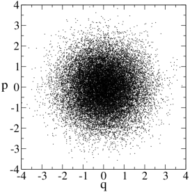
(a)

(b)

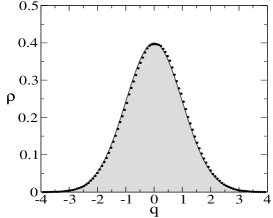
(c)

Figure 2: (a) The Poincaré section (p,q) for a harmonic oscillator coupled to the redesigned NHL thermostat (17). (b) The generated momentum density function (dots) as compared to the analytical result (solid cover filled in gray). (c) The same for the generated position density function.

A key difference between the NHL and RNHL schemes is that the latter relates the temperature control tool to the system $\mathrm{S_{ad}}$ rather than to the system $\mathrm{S}$, and the corresponding variable, $v$, must be Gaussian, according to the equations (17). Thus, it is important that the RNHL dynamical equations properly generate the Gaussian statistics of $v$ variable. Figure 3 shows the $v$-distribution function from simulations as compared with the exact analytical solution and indicates a good agreement between them.

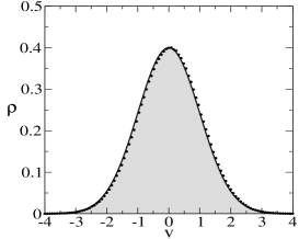
Figure 3: The density function for momentum $v$ (in the system $\mathrm{S_{ad}}$) from simulations (dots) as compared with the analytical solution (solid cover filled in gray).

V Conclusion

In conclusion, we emphasize that the method proposed in this work is based on the fundamental laws of statistical physics and offers a unified approach in developing stochastic and deterministic thermostats. For clarity of presentation we have illustrated our method using a few simple TEs and restricted our consideration by Markov dynamics. The presented method allowed us to obtain a wide spectrum of stochastic and deterministic dynamical systems with the invariant canonical measure. We note that the idea of presented method is general and adaptable to a variety of TEs so that it can be used to produce thermostats of novel types. For example the thermostat for the system with non-Markov dynamics, i.e. the one described by the equation $\boldsymbol{\nabla}H(x(t))\cdot\dot{x}(t)\propto\int_{0}^{t}dt^{\prime}G(t-t^{\prime})F(x(t^{\prime}),T)$. As a second example of new type of thermostats we can mention the one for the gradient dynamical system.

We realize that non-trivial new thermostats should be verified by test simulations. In our follow up work we will focus on these and other applications of the presented method.

References

• Allen and Tildesley (1989) M. P. Allen and D. J. Tildesley, Computer simulation of liquids (Oxford University Press, 1989).
• Frenkel and Smit (2002) D. Frenkel and B. Smit, Understanding molecular simulation: from algorithms to applications (Elsevier, 2002).
• Leimkuhler and Matthews (2015) B. Leimkuhler and C. Matthews, Molecular Dynamics: with deterministic and stochastic numerical methods (Springer, 2015).
• Tuckerman (2010) M. Tuckerman, Statistical mechanics: theory and molecular simulation (Oxford University Press, 2010).
• Jepps and Rondoni (2010) O. G. Jepps and L. Rondoni, J. Phys. A: Math. Gen. 43, 133001 (2010).
• Bussi et al. (2007) G. Bussi, D. Donadio,  and M. Parrinello, J. Chem. Phys. 126, 014101 (2007).
• Samoletov et al. (2007) A. Samoletov, C. Dettmann,  and M. Chaplain, J. Stat. Phys. 128, 1321 (2007).
• Leimkuhler et al. (2009) B. Leimkuhler, E. Noorizadeh,  and F. Theil, J. Stat. Phys. 135, 261 (2009).
• Samoletov et al. (2010) A. Samoletov, C. Dettmann,  and M. Chaplain, J. Chem. Phys. 132, 246101 (2010).
• Leimkuhler (2010) B. Leimkuhler, Phys. Rev. E 81, 026703 (2010).
• Bajars et al. (2011) J. Bajars, J. Frank,  and B. Leimkuhler, Eur. Phys. J. Special Topics 200, 131 (2011).
• Di Pierro et al. (2015) M. Di Pierro, R. Elber,  and B. Leimkuhler, J. Chem. Theory Comput. 11, 5624 (2015).
• Dittmar and Kusalik (2014) H. Dittmar and P. G. Kusalik, Phys. Rev. Lett. 112, 195701 (2014).
• Ness et al. (2016) H. Ness, A. Genina, L. Stella, C. Lorenz,  and L. Kantorovich, Phys. Rev. B 93, 174303 (2016).
• Dittmar and Kusalik (2016) H. R. Dittmar and P. G. Kusalik, J. Chem. Phys. 145, 134504 (2016).
• Stella et al. (2014) L. Stella, C. D. Lorenz,  and L. Kantorovich, Phys. Rev. B 89, 134303 (2014).
• Lepri et al. (1997) S. Lepri, R. Livi,  and A. Politi, Phys. Rev. Lett. 78, 1896 (1997).
• Pastorino et al. (2007) C. Pastorino, T. Kreer, M. Müller,  and K. Binder, Phys. Rev. E 76, 026706 (2007).
• Ciccotti and Ferrario (2016) G. Ciccotti and M. Ferrario, Mol. Simul. 42, 1385 (2016).
• Bianca (2012) C. Bianca, Phys. Life Rev. 9, 359 (2012).
• Samoletov and Vasiev (2013) A. Samoletov and B. Vasiev, Appl. Math. Lett. 26, 73 (2013).
• Chow et al. (2005) S.-M. Chow, N. Ram, S. M. Boker, F. Fujita,  and G. Clore, Emotion 5, 208 (2005).
• Tang et al. (2016) Y.-H. Tang, Z. Li, X. Li, M. Deng,  and G. E. Karniadakis, Macromolecules 49, 2895 (2016).
• Mones et al. (2015) L. Mones, A. Jones, A. W. Goetz, T. Laino, R. C. Walker, B. Leimkuhler, G. Csanyi,  and N. Bernstein, J. Comput. Chem. 36, 633 (2015).
• Fritz et al. (2011) D. Fritz, K. Koschke, V. A. Harmandaris, N. F. van der Vegt,  and K. Kremer, Phys. Chem. Chem. Phys. 13, 10412 (2011).
• Praprotnik et al. (2008) M. Praprotnik, L. D. Site,  and K. Kremer, Annu. Rev. Phys. Chem. 59, 545 (2008).
• Chen et al. (2016) C. Chen, N. Ding, C. Li, Y. Zhang,  and L. Carin, in Advances In Neural Information Processing Systems (2016) pp. 2937–2945.
• Leimkuhler and Shang (2016) B. Leimkuhler and X. Shang, SIAM J. Sci. Comput. 38, A712 (2016).
• Ding et al. (2014) N. Ding, Y. Fang, R. Babbush, C. Chen, R. D. Skeel,  and H. Neven, in Advances in Neural Information Processing Systems 27 (Curran Associates, Inc., 2014) pp. 3203–3211.
• Shang et al. (2015) X. Shang, Z. Zhu, B. Leimkuhler,  and A. J. Storkey, in Advances in Neural Information Processing Systems 28 (Curran Associates, Inc., 2015) pp. 37–45.
• Noid (2013) W. Noid, J. Chem. Phys. 139, 090901 (2013).
• Fukuda and Moritsugu (2017) I. Fukuda and K. Moritsugu, J. Phys. A: Math. Theor. 50, 015002 (2017).
• Fukuda and Moritsugu (2015) I. Fukuda and K. Moritsugu, J. Phys. A: Math. Theor. 48, 455001 (2015).
• Leimkuhler and Matthews (2013) B. Leimkuhler and C. Matthews, J. Chem. Phys. 138, 174102 (2013).
• Hoover (2012) W. G. Hoover, Computational statistical mechanics (Elsevier, 2012).
• Hoover (1985) W. G. Hoover, Phys. Rev. A 31, 1695 (1985).
• Nosé (1984) S. Nosé, Mol. Phys. 52, 255 (1984).
• Bussi et al. (2009) G. Bussi, T. Zykova-Timan,  and M. Parrinello, J. Chem. Phys. 130, 074101 (2009).
• Ruelle (2004) D. Ruelle, Phys. Today 57, 48 (2004).
• Rugh (1997) H. H. Rugh, Phys. Rev. Lett. 78, 772 (1997).
• Jepps et al. (2000) O. G. Jepps, G. Ayton,  and D. J. Evans, Phys. Rev. E 62, 4757 (2000).
• Hoover and Holian (1996) W. G. Hoover and B. L. Holian, Phys Lett A 211, 253 (1996).
• Uhlenbeck and Ford (1963) G. Uhlenbeck and G. Ford, Lectures in statistical mechanics. (AMS, Providence, Rhode Island, 1963).
• Novikov (1965) E. A. Novikov, Soviet Physics-JETP 20, 1290 (1965).
• Klyatskin (2005) V. I. Klyatskin, Dynamics of stochastic systems (Elsevier, 2005).
• Mattingly et al. (2002) J. C. Mattingly, A. M. Stuart,  and D. J. Higham, Stoch. Proc. Appl. 101, 185 (2002).
• Samoletov (1999) A. A. Samoletov, J. Stat. Phys. 96, 1351 (1999).
• Hoover et al. (2015) W. G. Hoover, J. C. Sprott,  and P. K. Patra, Phys Lett A 379, 2935 (2015)arXiv:1503.06749 [cond-mat.stat-mech] .
• Hoover et al. (2016) W. G. Hoover, J. C. Sprott,  and C. G. Hoover, Commun. Nonlinear Sci. Numer. Simul. 32, 234 (2016).
• Patra and Bhattacharya (2014) P. K. Patra and B. Bhattacharya, J. Chem. Phys. 140, 064106 (2014).
• Patra and Bhattacharya (2015) P. K. Patra and B. Bhattacharya, J. Chem. Phys. 142, 194103 (2015).
• Legoll et al. (2007) F. Legoll, M. Luskin,  and R. Moeckel, Arch. Ration. Mech. Anal. 184, 449 (2007).
• Martyna et al. (1992) G. J. Martyna, M. L. Klein,  and M. Tuckerman, The Journal of chemical physics 97, 2635 (1992).