Abstract

We define a particular combination of charge and heat currents that is decoupled with the heat current. This ‘heat-decoupled’ (HD) current can be transported by diffusion at long distances, when some thermo-electric conductivities and susceptibilities satisfy a simple condition. Using the diffusion condition together with the Kelvin formula, we show that the HD diffusivity can be same as the charge diffusivity and also the heat diffusivity. We illustrate that such mechanism is implemented in a strongly coupled field theory, which is dual to a Lifshitz gravity with the dynamical critical index $z=2$. In particular, it is exhibited that both charge and heat diffusivities build the relationship to the quantum chaos. Moreover, we study the HD diffusivity without imposing the diffusion condition. In some homogeneous holographic lattices, it is found that the diffusivity/chaos relation holds independently of any parameters, including the strength of momentum relaxation, chemical potential, or temperature. We also show a counter example of the relation and discuss its limited universality.

1 Introduction

One of the most mysterious phenomenon in condensed matters is the ubiquitous appearance of linear in temperature resistivity. In the materials with such ‘strange-metal’ hallmark, the quasiparticle picture is not applicable because the resistivity can cross the Mott-Ioffe-Regel limit [1, 2]. It has been long suggested [3, 4] that the transport in strange metals is controlled by the ‘Planckian dissipation’—the temperature in units of time through Planck’s constant: $\tau_{\mathrm{P}}\sim\hbar/(k_{\mathrm{B}}T)$, but the explicit framework has not been built up.

In [5], Hartnoll has pointed out that when the momentum decays quickly, the collective diffusion of charge and energy controls the strange-metal transport. Inspired by the putative bound on the ratio of shear viscosity to entropy density [6], he proposed that the eigenvalues of diffusive matrix are lower bounded by the Planckian dissipation and Fermi velocity. Translating by the Einstein relation and neglecting some thermoelectric effect, he argued that the saturation of the diffusion bound may be responsible for the ubiquity of high-temperature regimes in metals with $T$-linear resistivity.

The theory of incoherent metals is insightful, but there are several issues which deserve to be explored. First, the diffusion bound can be violated in various situations [7, 8, 9, 10]. Second, some strange metals are relatively clean and their thermoelectric effect may not be especially small. Third, the characteristic velocity $v_{\mathrm{P}}$ is taken as the Fermi velocity $v_{\mathrm{F}}$, which may not be well defined in strongly coupled systems. To address the last issue, the butterfly velocity $v_{\mathrm{B}}$ that quantifies the speed of chaos propagation has been proposed as a natural replacement [11, 12]. Actually, an interesting relation has been found by holography between the charge diffusivity and the quantum chaos which is characterized by $v_{\mathrm{B}}$ and $\tau_{\mathrm{L}}$. Here $\tau_{\mathrm{L}}$ is the Lyapunov time that is expected to indicate the Planckian dissipation in non-quasiparticle systems [13, 14, 15, 16, 17]. However, in addition to the non-universal prefactors that occur in special cases [18, 19], the application of charge diffusivity/chaos relation is limited since the particle-hole symmetry must be imposed. As a result, the relation does not appear in the normal state of cuprates. On the other hand, the relation between the thermal diffusivity and chaos seems to be more robust [12, 20, 21, 22, 23, 24], but it cannot be directly translated into the statement of resistivity.

Nevertheless, by a recent local optical measurements of thermal diffusivity on underdoped YBCO (an ortho-II YBa₂Cu₃O_6.60 and an ortho-III YBa₂Cu₃O_6.75) crystals, it was found that the thermal anisotropy is almost identical to the value of the electrical resistivity anisotropy and starts to decrease sharply below the charge order transition [25]. The experiment was interpreted that the non-quasiparticle transport is dominated by the collective diffusion of electron-phonon ‘soup’. In particular, it led to the conjecture that both charge and heat diffusivities saturate the proposed bounds [25, 26].

To understand how the collective diffusion could be relevant to the intrinsic mechanism for robust metallic transport that is complicated by the extrinsic processes for momentum relaxation, it would be promising to search hints in clean systems. Indeed, in a conformal field theory (CFT) with charge doping, Davison, Goutéraux and Hartnoll (DGH) have isolated a diffusive mode by hydrodynamics [27, 28], which is carried by a particular combination of the charge and heat currents. The DGH mode can likely be considered intrinsic, because the DGH current is decoupled with momentum in the conformal fluid and the DGH conductivity is universal for some clean holographic theories [29]. However, the DGH mode has not been studied when the translation symmetry is broken, partially because a simple proposal to include slow momentum relaxation in hydrodynamics [30] is inconsistent with the holographic models [28, 31] and the fast momentum relaxation invalidates the hydrodynamics essentially.

In this paper, we will explore the collective diffusion of charge and energy and its relationship to quantum chaos in terms of the gauge/gravity duality with momentum relaxation. At the beginning, we will show that there is a universal bound for thermo-electric transport. The bound is trivial, except that its saturation indicates the decoupling between the heat current and a particular combination of charge and heat currents. The ‘heat-decoupled’ (HD) current is nothing but the DGH current in most of homogeneous holographic lattices. Without relying on the hydrodynamics, we will verify that the HD current can be transported by diffusion at long distances, when some thermo-electric conductivities and susceptibilities satisfy a simple condition. Then we will study the HD mode by combining the diffusion condition and the Kelvin formula [32]. Note that the Kelvin formula arises if the static limit is taken before the thermodynamic limit in the evaluation of Onsager coefficients [32]. It provides a good approximate (sometimes even exact) expression of the thermopower in various contexts including strongly correlated systems, such as the fractional quantum Hall states [32], high temperature superconductors [32, 33, 34], and the homogeneous Sachdev-Ye-Kitaev model [19]. As a result, we will point out that not only the heat diffusivity but also the charge diffusivity can be identified with the HD diffusivity. Furthermore, in a Lifshitz gravity with the dynamical critical index $z=2$, we will illustrate that the diffusion condition and the Kelvin formula can be realized. Meanwhile, the HD diffusivity exhibits the relationship to the quantum chaos and is equal to both charge and heat diffusivities.

In the thermo-electric systems that we care about, the fluctuations of charge and energy are coupled and hence they do not satisfy separate diffusion equations in general. Accordingly, the charge and energy diffusivities do not correspond to any eigenvalues of the diffusivity matrix. However, they still can be well defined (by their Einstein relation) and would imply interesting physics. This inspires us to study the diffusion constant of HD mode, but without imposing any diffusion condition. In other words, the HD mode is no longer purely diffusive. We will exhibit that the diffusivity/chaos relation is respected exactly in various homogeneous holographic lattices. This is different with previous results in references, where the diffusivity/chaos relation always requires certain limits on the parameters, including the particle-hole symmetry [11, 9], strong momentum relaxation [12, 21, 22], or low temperature [20, 23]. However, the relation is not universal and we will show a counter example. The limited universality and implication will be discussed.

2 Heat-decoupled current

The thermo-electric transport is characterized by three conductivities: electrical $\sigma$, thermal $\bar{\kappa}$, and thermoelectric $\alpha$. They reflect the response of the charge and heat currents to small gradients of temperature and chemical potential,

$$\left(\begin{array}[]{c}J\\ J^{Q}\end{array}\right)=\left(\begin{array}[]{cc}\sigma&T\alpha\\ T\alpha&T\bar{\kappa}\end{array}\right)\left(\begin{array}[]{c}-\nabla\mu\\ -\nabla T/T\end{array}\right).$$ (1)

The DGH current is defined by a particular combination of charge and heat currents [27]

$$J^{\mathrm{DGH}}\equiv\frac{sTJ-\rho J^{Q}}{sT+\rho\mu},$$ (2)

where $\rho$ is the charge density and $\mu$ is the chemical potential. Now we construct a general linear combination but write it as the DGH-like form for comparison

$$\bar{J}^{\mathrm{DGH}}\equiv\frac{sTJ-\bar{\rho}J^{Q}}{sT+\bar{\rho}\mu}.$$ (3)

In the present, $\bar{\rho}$ is an arbitrary quantity with the dimension of charge density. The current-current correlation can be calculated by

$$\bar{\sigma}_{\mathrm{DGH}}\equiv\left\langle\bar{J}^{\mathrm{DGH}}\bar{J}^{\mathrm{DGH}}\right\rangle=\frac{T(\bar{\rho}^{2}\bar{\kappa}+s^{2}T\sigma-2\bar{\rho}sT\alpha)}{\left(sT+\bar{\rho}\mu\right)^{2}}.$$ (4)

We reorganize the numerator of Eq. (4):

$$T(\bar{\rho}^{2}\bar{\kappa}+s^{2}T\sigma-2\bar{\rho}sT\alpha)$$ (5)

$$= \left(\sigma-\frac{T\alpha^{2}}{\bar{\kappa}}\right)\left(sT\right)^{2}+\frac{T}{\bar{\kappa}}\left(sT\alpha-\bar{\rho}\bar{\kappa}\right)^{2}.$$

In the dc limit, the last term in Eq. (5) is non-negative, so we immediately obtain a universal bound

$$\bar{\sigma}_{\mathrm{DGH}}\geq\sigma_{0}\frac{\left(sT\right)^{2}}{\left(sT+\bar{\rho}\mu\right)^{2}},$$ (6)

where $\sigma_{0}\equiv\sigma-T\alpha^{2}/\bar{\kappa}$ denotes the electric conductivity at zero heat current. The bound is almost trivial. The only interesting point is that, due to

$$\left\langle\bar{J}^{\mathrm{DGH}}J^{Q}\right\rangle=\frac{\bar{\rho}\bar{\kappa}-sT\alpha}{\mu\left(sT+\bar{\rho}\mu\right)},$$ (7)

the bound is saturated when the general current is decoupled with the heat current. Hereafter, we will focus on the HD current

$$J^{\mathrm{HD}}\equiv\left.\bar{J}^{\mathrm{DGH}}\right|_{\bar{\rho}=sT\alpha/\bar{\kappa}}=\frac{\bar{\kappa}J-\alpha J^{Q}}{\bar{\kappa}+\alpha\mu}.$$ (8)

One can find that the HD current is equal to the DGH current in most of homogeneous holographic lattices which have

$$\rho=sT\alpha/\bar{\kappa}.$$ (9)

However, this relation does not hold when the momentum relaxation is inhomogeneous [36] or involves some non-minimal coupling [37, 10, 22]. In these cases, the HD current is different with the DGH current and might be viewed as an extension.

3 Diffusive mode

Suppose that the energy and the charge are conserved. The HD current respects the continuous equation

$$\frac{\partial}{\partial t}\delta Q^{\mathrm{HD}}+\nabla\cdot J^{\mathrm{HD}}=0,$$ (10)

and carries a particular combination of charge and energy

$$\delta Q^{\mathrm{HD}}\equiv\delta\rho-\frac{\alpha}{\bar{\kappa}+\alpha\mu}\delta\epsilon,$$ (11)

where we denote $\epsilon$ as the energy density. Using the definition of conductivities (1), the continuous equation (10), and the thermodynamic identities

$$\nabla\rho = \chi\nabla\mu+\zeta\nabla T,$$

$$\nabla\epsilon = (T\zeta+\mu\chi)\nabla\mu+(\mu\zeta+c_{\mu})\nabla T,$$ (12)

with the susceptibilities defined by derivatives of pressure

$$\chi\equiv\partial^{2}p/\partial\mu^{2},\;\zeta\equiv\partial^{2}p/\partial\mu\partial T,\;c_{\mu}\equiv T\partial^{2}p/\partial T^{2},$$ (13)

one can prove at long distances

$$\frac{\partial}{\partial t}\delta Q^{\mathrm{HD}}=D_{\mathrm{HD}}\left[\nabla^{2}\delta Q^{\mathrm{HD}}+C\nabla^{2}\rho\right],$$ (14)

where we have defined

$$D_{\mathrm{HD}} \equiv \frac{\zeta}{\alpha}\frac{\bar{\kappa}\sigma-T\alpha^{2}}{c_{\mu}\chi-T\zeta^{2}},$$ (15)

$$C \equiv 1-\frac{\alpha\mu}{\bar{\kappa}+\alpha\mu}\frac{c_{\mu}+\zeta\mu}{\zeta\mu}.$$ (16)

Following Ref. [38], the diffusion equation

$$\frac{\partial}{\partial t}\delta Q^{\mathrm{HD}}=D_{\mathrm{HD}}\nabla^{2}\delta Q^{\mathrm{HD}}$$ (17)

can be constructed, provided that $C=0$, which means

$$\bar{\kappa}/c_{\mu}=\alpha/\zeta.$$ (18)

At this time, the diffusion constant can be written as

$$\bar{D}_{\mathrm{HD}}\equiv\left.D_{\mathrm{HD}}\right|_{C=0}=\frac{\bar{\kappa}\sigma-T\alpha^{2}}{\bar{\kappa}\chi-T\alpha\zeta}.$$ (19)

Some remarks are in order. First, the diffusion condition (18) can be understood as a special balance between the thermoelectric conductivity $\alpha$ and susceptibility $\zeta$. The thermoelectric balance is reminiscent of the Kelvin formula which can be written as $\sigma/\chi=\alpha/\zeta$. The Kelvin formula can be derived by requesting that the density gradient vanishes [34]. At that time, Eq. (14) becomes the diffusion equation without requiring any additional conditions. Second, usually the diffusion constant $D_{\mathrm{HD}}$ is not equal to the charge diffusivity $D_{\mathrm{C}}\equiv\sigma/\chi$ or thermal diffusivity $D_{\mathrm{T}}\equiv\kappa/c_{\rho}$, where $\kappa\equiv\bar{\kappa}-T\alpha^{2}/\sigma$ and $c_{\rho}\equiv c_{\mu}-T\zeta^{2}/\chi$. However, by recasting Eq. (15) as $D_{\mathrm{HD}}=D_{\mathrm{C}}D_{\mathrm{T}}\zeta/\alpha$ and invoking the Kelvin formula $D_{\mathrm{C}}=\alpha/\zeta$, one can find $D_{\mathrm{HD}}=D_{\mathrm{T}}$. Furthermore, the combination of Eq. (18) and the Kelvin formula leads to $\bar{D}_{\mathrm{HD}}=D_{\mathrm{C}}=D_{\mathrm{T}}$. Third, $D_{\mathrm{HD}}=\sigma D_{\mathrm{T}}\zeta/\left(\chi\alpha\right)$ apparently involves $\chi$ and $\zeta$. In the holographic models, they depend on the full bulk geometry in general. However, they can be cancelled in $D_{\mathrm{HD}}$ due to $\zeta/\chi=\left(\partial s/\partial\rho\right)_{T}$, which is indeed related to the thermodynamics of black holes [20]. At last, it is instructive to clarify the relation between the HD current with the diffusion condition and the decoupled thermo-electric currents which are transported by diffusion [28, 39], see Appendix A. In the following, we will reveal a general and exact relation between $D_{\mathrm{HD}}$ and $v_{\mathrm{B}}^{2}\tau_{\mathrm{L}}$ in various holographic models. In particular, the diffusion condition (18) and the Kelvin formula both hold in a model of Lifshitz gravity with $z=2$, leading to $D_{\mathrm{C}}=D_{\mathrm{T}}=v_{\mathrm{B}}^{2}\tau_{\mathrm{L}}$.

4 Holographic models

4.1 Einstein-Maxwell-axion

A simple holographic framework with momentum relaxation was presented in [40]. The model contains linear axions $\chi_{i}$ along spatial directions. We consider the four-dimensional Einstein-Maxwell-axion (EMA) theory,

$$S_{\mathrm{bulk}}=\int d^{4}x\sqrt{-g}{\Big{[}}R+6-\frac{1}{4}F^{2}-\frac{1}{2}\sum\limits_{i=1}^{2}\left(\partial\chi_{i}\right)^{2}{\Big{]}}.$$ (20)

Here the AdS radius $L$ and the Newton constant $16\pi G_{N}$ are set to unity. The equations of motion (EOM) derived from the action has an isotropic background solution, in which $\chi_{i}=\beta x_{i}$ with the disorder parameter $\beta$ [40]. Suppose that the horizon locates at $r_{+}$. The Hawking temperature and entropy density are

$$T=\frac{1}{4\pi}\left(3r_{+}-\frac{2\beta^{2}+\rho^{2}/r_{+}^{2}}{4r_{+}}\right),\;s=4\pi r_{+}^{2},$$ (21)

from which two thermodynamic response functions can be derived

$$\left(\frac{\partial s}{\partial T}\right)_{\rho}=\frac{128\pi^{2}r_{+}^{5}}{3\rho^{2}+2\beta^{2}r_{+}^{2}+12r_{+}^{4}},\;\left(\frac{\partial s}{\partial\rho}\right)_{T}=\frac{16\pi\rho r_{+}^{2}}{3\rho^{2}+2\beta^{2}r_{+}^{2}+12r_{+}^{4}}.$$ (22)

By building up the conserved currents and invoking the sources that are linear in time, Donos and Gauntlett derived the thermo-electric conductivities analytically [35]:

$$\sigma=1+\frac{4\pi\rho^{2}}{s\beta^{2}},\;\alpha=\frac{4\pi\rho}{\beta^{2}},\;\bar{\kappa}=\frac{4\pi sT}{\beta^{2}}.$$ (23)

Using Eq. (22), Eq. (23), and $\zeta/\chi=\left(\partial s/\partial\rho\right)_{T}$, the diffusion constant (15) can be calculated. The result is simple:

$$D_{\mathrm{HD}}=\frac{1}{2r_{+}}.$$ (24)

We need to study the quantum chaos. The onset of chaos is characterized by the Lyapunov time $\tau_{\mathrm{L}}$ and the butterfly velocity $v_{\mathrm{B}}$. They can be calculated by constructing a shock wave near the black hole [41, 42, 43, 44, 45]. For the EMA model, they are [11, 12]

$$\tau_{\mathrm{L}}=\frac{1}{2\pi T},\;v_{\mathrm{B}}^{2}=\frac{\pi T}{r_{+}}.$$ (25)

Remarkably, we have found an exact diffusivity/chaos relation

$$D_{\mathrm{HD}}=v_{\mathrm{B}}^{2}\tau_{\mathrm{L}}.$$ (26)

As a comparison, we write down the ratio between $D_{\mathrm{T}}$ and $v_{\mathrm{B}}^{2}\tau_{\mathrm{L}}$

$$\frac{D_{\mathrm{T}}}{v_{\mathrm{B}}^{2}\tau_{\mathrm{L}}}=\frac{3\rho^{2}+2r_{+}^{2}\beta^{2}+12r_{+}^{4}}{4\left(\rho^{2}+r_{+}^{2}\beta^{2}\right)}.$$ (27)

4.2 Non-relativistic scaling

We have interest on an Einstein-Maxwell-Axion-Dilaton (EMAD) theory studied in [46, 47]

$$S_{\mathrm{bulk}}=\int d^{4}x\sqrt{-g}\left[R+V\left(\phi\right)-\frac{1}{2}\left(\partial\phi\right)^{2}-\frac{1}{4}\sum\limits_{i=1}^{2}Z_{i}\left(\phi\right)F_{(i)}^{2}-\frac{1}{2}Y\left(\phi\right)\sum\limits_{i=1}^{2}\left(\partial\chi_{i}\right)^{2}\right],$$ (28)

where all the functions of the dilaton are assumed to have the exponential form

$$V\left(\phi\right)=-2\Lambda e^{\lambda_{0}\phi},\;Z_{1}\left(\phi\right)=e^{\lambda_{1}\phi},\;Z_{2}\left(\phi\right)=e^{\lambda_{2}\phi},\;Y\left(\phi\right)=e^{\lambda_{3}\phi},$$ (29)

with several parameters $\Lambda$ and $\lambda_{i}$ ($i=0,1,2,3$). This theory admits Lifshitz-like, hyperscaling violating, analytical black-brane solutions. The line element is given by

$$ds^{2}=r^{\theta}\left[-r^{2z}f\left(r\right)dt^{2}+\frac{dr^{2}}{r^{2}f\left(r\right)}+r^{2}\left(dx^{2}+dy^{2}\right)\right],$$ (30)

where the blackness factor is

$$f\left(r\right)=1-\frac{m}{r^{\theta+z+2}}+\frac{\beta^{2}}{\left(\theta+2\right)\left(z-2\right)}\frac{1}{r^{2z+\theta}}+\frac{q_{2}^{2}}{2\left(\theta+2\right)\left(z+\theta\right)}\frac{1}{r^{2(z+\theta+1)}}.$$ (31)

We have denoted the dynamical critical index as $z$ and the hyperscaling violating factor $\theta$. Besides the usual electromagnetic field, there is an additional Maxwell field which is necessary for $z\neq 1$. Two Maxwell fields have the charges $\left(q_{1},q_{2}\right)$, respectively. We will impose the physical condition that the first U(1) current is vanishing. Then the charge density is $\rho=q_{2}$. The parameters $\Lambda$, $\lambda_{i}$, and $q_{1}$ are all determined by $z$ and $\theta$. For instance, $q_{1}=\sqrt{2\left(z-1\right)\left(z+\theta+2\right)}$. In [47], it has been pointed out that the black-brane solution is divergent when $z=2$, indicating the logarithmic behavior. The blackness factor then becomes

$$f\left(r\right)=1-\frac{1}{r^{\theta+4}}\left(m+\frac{\beta^{2}}{\theta+2}\log r\right)+\frac{q_{2}^{2}}{2\left(\theta+2\right)^{2}}\frac{1}{r^{2(\theta+3)}}.$$ (32)

Using the black-brane solutions, the temperature and entropy density can be written as

$$T=\frac{z+\theta+2}{4\pi}r_{+}^{z}-\frac{q_{2}^{2}+2\beta^{2}r_{+}^{\theta+2}}{8\pi\left(\theta+2\right)r_{+}^{z+2\theta+2}},\;s=4\pi r_{+}^{\theta+2},$$ (33)

which is effective even for $z=2$. They can lead to two response functions

$$\left(\frac{\partial s}{\partial T}\right)_{\rho} = \frac{32\pi^{2}r_{+}^{z+3\theta+4}(\theta+2)^{2}}{q_{2}^{2}\left(z+2\theta+2\right)+2r_{+}^{\theta+2}\left[\left(z+\theta\right)\beta^{2}+r_{+}^{2z+\theta}z\left(\theta+2\right)\left(z+\theta+2\right)\right]},$$

$$\;\left(\frac{\partial s}{\partial\rho}\right)_{T} = \frac{8\pi q_{2}r_{+}^{\theta+2}(\theta+2)}{q_{2}^{2}\left(z+2\theta+2\right)+2r_{+}^{\theta+2}\left[\left(z+\theta\right)\beta^{2}+r_{+}^{2z+\theta}z\left(\theta+2\right)\left(z+\theta+2\right)\right]}.$$ (34)

From Ref. [46], the dc thermo-electric conductivities can be read off,

$$\sigma=r_{+}^{2z+\theta-2}+\frac{q_{2}^{2}r_{+}^{2z-\theta-2}}{\beta^{2}r_{+}^{2-\theta}+q_{1}^{2}r_{+}^{2z+2}},\;\alpha=\frac{4\pi q_{2}r_{+}^{2z}}{\beta^{2}r_{+}^{2-\theta}+q_{1}^{2}r_{+}^{2z+2}},\;\bar{\kappa}=\frac{16\pi^{2}Tr_{+}^{2z+\theta+2}}{\beta^{2}r_{+}^{2-\theta}+q_{1}^{2}r_{+}^{2z+2}}.$$ (35)

To obtain the quantities in chaos, we study a shock-wave metric

$$ds^{2}=A(uv)dudv+V(uv)d\vec{x}^{2}-A(uv)\delta\left(u\right)h(t,\vec{x})du^{2},$$ (36)

which is generated by releasing a particle from the boundary at $\vec{x}=0$. From the EOM, one can obtain the solution of $h(t,\vec{x})$ at later time and large distance. Then we can extract the Lyapunov time $\tau_{\mathrm{L}}=1/\left(2\pi T\right)$ and the butterfly velocity $v_{\mathrm{B}}=2\pi T/m$, with the screening length $m$ given by

$$m^{2}=\frac{2}{A(0)}\left.\frac{\partial V(uv)}{\partial(uv)}\right|_{u=0}.$$ (37)

Equation (37) is same as the one in [11], indicating that the additional Maxwell field does not change the form of the screening length. Translating the Kruskal coordinates into Schwarzschild coordinates, we have

$$v_{\mathrm{B}}^{2}=\frac{2\pi Tr_{+}^{z-2}}{\theta+2}\mathcal{.}$$ (38)

Using Eq. (34) and Eq. (35), one can calculate the diffusion constant (15)

$$D_{\mathrm{HD}}=\frac{r_{+}^{z-2}}{\theta+2}.$$ (39)

Thus, we have the robust relation $D_{\mathrm{HD}}=v_{\mathrm{B}}^{2}\tau_{\mathrm{L}}$ for the generic $z$ and $\theta$. For comparison, the ratio between $D_{\mathrm{T}}$ and $v_{\mathrm{B}}^{2}\tau_{\mathrm{L}}$ depends on $z$ and $\theta$:

$$\frac{D_{\mathrm{T}}}{v_{\mathrm{B}}^{2}\tau_{\mathrm{L}}}=\frac{\left(z+2\theta+2\right)q_{2}^{2}+2r_{+}^{\theta+2}\left[\left(z+\theta\right)\beta^{2}+r_{+}^{2z+\theta}z\left(\theta+2\right)\left(z+\theta+2\right)\right]}{2\left(\theta+2\right)\left[q_{2}^{2}+r_{+}^{\theta+2}\beta^{2}+2r_{+}^{2z+2\theta+2}\left(z-1\right)\left(z+\theta+2\right)\right]}.$$ (40)

Let’s focus on the special case with $z=2$. From Eq. (34) and Eq. (35), one can see

$$\frac{\alpha}{\sigma}=\left(\frac{\partial s}{\partial\rho}\right)_{T},$$ (41)

which implies that the Kelvin formula $\sigma/\chi=\alpha/\zeta$ holds and $D_{\mathrm{HD}}=D_{\mathrm{T}}$. Furthermore, we have interest on the case with $\theta=0$. To be clear, we rewrite the temperature and entropy density, and also invoke the chemical potential:

$$T=\frac{1}{\pi}\left(r_{+}^{2}-\frac{2\beta^{2}+\rho^{2}/r_{+}^{2}}{16r_{+}^{2}}\right),\;s=4\pi r_{+}^{2},\;\mu=\frac{\rho}{2r_{+}^{2}}.$$ (42)

The last equation is necessary to calculate the quantities $\chi$, $\zeta$, and $c_{\mu}$. One can find that the diffusion condition (18) is obeyed. Collecting all the results in the exceptional case with $z=2$ and $\theta=0$, we have a series of equalities

$$D_{\mathrm{HD}}=\bar{D}_{\mathrm{HD}}=D_{\mathrm{C}}=D_{\mathrm{T}}=v_{\mathrm{B}}^{2}\tau_{\mathrm{L}}.$$ (43)

4.3 High curvature

The higher derivative corrections appear generally in any quantum gravity theory from quantum or stringy effects. These corrections may be holographic dual to $1/N$ or $1/\lambda$ corrections in some gauge theories, allowing independent values of two central charges $a$ and $c$. This is in contrast to the standard $\mathcal{N}$=4 super Yang-Mills theory where $a=c$, hence likely underpinning the violation of viscosity bound. Actually, the Gauss-Bonnet (GB) correction has been treated as a dangerous source of violation for the feature that is universal in Einstein gravity [48, 49].

Consider the GB correction to the EMA theory, that is

$$S_{\mathrm{bulk}} = \int d^{5}x\sqrt{-g}{\Big{[}}R+12-\frac{1}{4}F^{\mu\nu}F_{\mu\nu}-\frac{1}{2}\sum\limits_{i=1}^{3}\left(\partial\chi_{i}\right)^{2}$$ (44)

$$+\frac{\tilde{\alpha}}{2}\left(R^{2}-4R^{\mu\nu}R_{\mu\nu}+R_{\mu\nu\lambda\rho}R^{\mu\nu\lambda\rho}\right){\Big{]}},$$

where $\tilde{\alpha}$ is the GB coupling constant. The black-brane solution with $\chi_{i}=\beta x_{i}$ has been derived in [50]. The temperature and entropy density can be written as

$$T=\frac{L_{\mathrm{eff}}}{\pi}\left(r_{+}-\frac{\beta^{2}}{8r_{+}}-\frac{\rho^{2}}{24r_{+}^{5}}\right),\;s=4\pi r_{+}^{3}.$$ (45)

Here $L_{\mathrm{eff}}^{2}=\frac{1+\sqrt{1-4\tilde{\alpha}}}{2}$ is the square of the effective AdS radius. Taking the derivatives of the entropy density, the two response functions read:

$$\left(\frac{\partial s}{\partial T}\right)_{\rho}=\frac{1}{L_{\mathrm{eff}}}\frac{288\pi^{2}r_{+}^{8}}{5\rho^{2}+3\beta^{2}r_{+}^{4}+24r_{+}^{6}},\;\left(\frac{\partial s}{\partial\rho}\right)_{T}=\frac{24\pi\rho r_{+}^{3}}{5\rho^{2}+3\beta^{2}r_{+}^{4}+24r_{+}^{6}}.$$ (46)

We also need the thermo-electric conductivities [50]

$$\sigma=r_{+}+\frac{4\pi\rho^{2}}{s\beta^{2}},\;\alpha=\frac{4\pi\rho}{\beta^{2}},\;\bar{\kappa}=\frac{4\pi sT}{\beta^{2}}.$$ (47)

Using Eq. (46) and Eq. (47), the diffusion constant (15) can be calculated as

$$D_{\mathrm{HD}}=\frac{L_{\mathrm{eff}}}{3r_{+}}.$$ (48)

The butterfly effect for GB gravity has been studied in [42]. We will repeat the calculation but involve the linear axions. Release a particle from the boundary and consider the five-dimensional shock-wave metric

$$ds^{2}=A(uv)dudv+V(uv)d\vec{x}^{2}-A(uv)\delta\left(u\right)h(t,\vec{x})du^{2}.$$ (49)

Using the EOM, one can derive the solution of $h(t,\vec{x})$ at later time and large distance, which in turn gives the Lyapunov time $\tau_{\mathrm{L}}=1/\left(2\pi T\right)$ and the butterfly velocity $v_{\mathrm{B}}=2\pi T/m$, with the screening length $m$ given by

$$m^{2}=\frac{3}{A(0)}\left.\frac{\partial V(uv)}{\partial(uv)}\right|_{u=0}.$$ (50)

Under the Schwarzschild coordinates, one can read

$$v_{\mathrm{B}}^{2}=2\pi T\frac{L_{\mathrm{eff}}}{3r_{+}}\mathcal{.}$$ (51)

Then we build the diffusivity/chaos relation $D_{\mathrm{HD}}=v_{\mathrm{B}}^{2}\tau_{\mathrm{L}}$ again. The ratio between $D_{\mathrm{T}}$ and $v_{\mathrm{B}}^{2}\tau_{\mathrm{L}}$ can be given by

$$\frac{D_{\mathrm{T}}}{v_{\mathrm{B}}^{2}\tau_{\mathrm{L}}}=\frac{5\rho^{2}+3r_{+}^{4}\beta^{2}+24r_{+}^{6}}{6\left(\rho^{2}+r_{+}^{4}\beta^{2}\right)}.$$ (52)

4.4 Anisotropy

Spatially anisotropic black-brane is the first example that yields the violation of viscosity bound in Einstein gravity [51]. A careful examination of the diffusivity/chaos relation in such anisotropic model is worthwhile. In [52, 53], a R-charged version of the spatially anisotropic black-brane solution was derived via nonlinear Kaluza-Klein reduction of type-IIB supergravity to five dimensions, which leads to the presence of an Abelian field in the action. The introduction of the $U(1)$ gauge field breaks the $SO(6)$ symmetry and thus leads to the excitations of the Kaluza-Klein modes. Consider the reduced theory that is described by a five-dimensional EMAD action

$$S_{\mathrm{bulk}}=\int d^{5}x\sqrt{-g}\left[R+12-\frac{1}{4}F^{\mu\nu}F_{\mu\nu}-\frac{1}{2}\left(\partial\phi\right)^{2}-\frac{1}{2}e^{2\phi}\left(\partial\chi\right)^{2}\right].$$ (53)

There is an anisotropic solution

$$ds^{2}=-h(r)dt^{2}+\frac{1}{f(r)}dr^{2}+g_{11}(r)dx_{1}^{2}+g_{33}(r)\left(dx_{2}^{2}+dx_{3}^{2}\right)$$ (54)

$$A=A_{t}(r)dt,\;\phi=\phi(r),\;\chi=\beta x_{1},$$ (55)

which has been found numerically in [52]. Note that the strength of anisotropy and disorder are both characterized by the single parameter $\beta$. The analytical solution with small $\beta$ has also been obtained, see Appendix D in [52]. We write them as follows:

$$h(r) = \frac{1}{u^{2}}e^{-\frac{\phi(u)}{2}}\mathcal{B}(u)\mathcal{F}(u),\;f(r)=\frac{1}{u^{2}}e^{\frac{\phi(u)}{2}}\mathcal{F}(u),$$

$$g_{11}(r) = \frac{1}{u^{2}}e^{-\frac{3\phi(u)}{2}},\;g_{33}(r)=\frac{1}{u^{2}}e^{-\frac{\phi(u)}{2}},$$ (56)

where $u\equiv 1/r$. The three functions $\left(\mathcal{F},\mathcal{B},\phi\right)$ are given by

$$\mathcal{F}(u) = 1-\frac{u^{4}}{u_{+}^{4}}-\frac{1}{12}\rho^{2}u^{4}u_{+}^{2}+\frac{\rho^{2}u^{6}}{12}+\beta^{2}\mathcal{F}_{2}(u)+\mathcal{O(}\beta^{4}\mathcal{),}$$

$$\mathcal{B}(u) = 1+\beta^{2}\mathcal{B}_{2}(u)+\mathcal{O(}\beta^{4}\mathcal{),}$$

$$\phi(u) = \beta^{2}\phi_{2}(u)+\mathcal{O(}\beta^{4}\mathcal{),}$$ (57)

where $\left(\mathcal{F}_{2},\mathcal{B}_{2},\phi_{2}\right)$ can be read off from Eq. (135) in [52] with the replacement for our convention

$$\left(a,u_{\mathrm{H}},q^{2}\right)\rightarrow\left(\beta,u_{+},\frac{\rho^{2}u_{+}^{6}}{12}\right).$$ (58)

To be simple, we will use the analytical solution to study the diffusion and chaos, instead of the numerical solution. The two thermodynamic quantities are

$$T=\frac{\sqrt{\mathcal{B}(u_{+})}\mathcal{F}^{\prime}(u_{+})}{4\pi},\;s=4\pi u_{+}^{-3}e^{-\frac{5}{4}\phi(u_{+})}.$$ (59)

We need the thermo-electric conductivities, which can be found in [53]:

$$\sigma=\frac{g_{33}(u_{+})}{\sqrt{g_{11}(u_{+})}}+\frac{4\pi\rho^{2}}{e^{2\phi(r_{+})}\beta^{2}s},\;\alpha=\frac{4\pi\rho}{e^{2\phi(r_{+})}\beta^{2}},\;\bar{\kappa}=\frac{4\pi sT}{e^{2\phi(r_{+})}\beta^{2}}.$$ (60)

We will study the anisotropic chaos. The present model is the five-dimensional anisotropic model with an axion. Note that the butterfly velocity in the four-dimensional model with anisotropic lattices has been studied recently in [45]. Consider a shock-wave metric

$$ds^{2} = A(uv)dudv+V_{1}(uv)dx_{1}^{2}+V_{3}(uv)\left(dx_{2}^{2}+dx_{3}^{2}\right)$$ (61)

$$-A(uv)\delta\left(u\right)h(t,\vec{x})du^{2}.$$

One can find that the previous form of Lyapunov time $\tau_{\mathrm{L}}=1/\left(2\pi T\right)$ and butterfly velocity $v_{\mathrm{B}}^{2}=2\pi T/m$ is not changed, but the screening length is affected by anisotropy:

$$m^{2}=\frac{V_{1}(0)}{A(0)}\left.\sum_{i=1}^{3}\frac{V_{i}^{\prime}(0)}{V_{i}(0)}\right|_{u=0}.$$ (62)

Using the analytical expression of the background solution and conductivities, we display in Figure 1 the temperature dependence of the butterfly velocity and two diffusivity/chaos relation for comparison. Typically, we fix the parameter $\beta/\mu=0.1$ and cut off the regime $T/\mu\ll 0.1$ in which $\beta\gg T$ and hence the analytical solution is not reliable. Other values of the parameter do not lead to the qualitative difference. As a result, one can see $D_{\mathrm{HD}}=v_{\mathrm{B}}^{2}\tau_{\mathrm{L}}$.

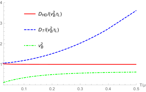
Figure 1: Diffusivty/chaos relation in the anisotropic holographic model with $\beta/\mu=0.1$.

4.5 Non-minimal coupling

In all aforementioned models, the translation-symmetry breaking sector is minimally coupled to the gravitational and electromagnetic sectors. There are novel models which involve the non-minimal coupling between the Maxwell term and the axions [37, 10]. We will focus on one of these models, i.e. the model 1 in [37]. Compared with others, its conductivities are more trivial, leading to the situation with $J^{\mathrm{HD}}\neq J^{\mathrm{DGH}}$. Actually, this model is so distinctive that it breaks various bounds on the viscosity [6], electric conductivity [54] and charge diffusivity [5]. The action is given by

$$S_{\mathrm{bulk}}=\int d^{4}x\sqrt{-g}\left(R+6-\frac{1}{4}F^{2}-\frac{1}{4}\mathcal{J}\mathrm{Tr}\left[\mathcal{X}F^{2}\right]-\mathrm{Tr}\left[\mathcal{X}\right]\right),$$ (63)

where $\mathcal{J}$ is the coupling constant and

$$\mathcal{X}_{\;\nu}^{\mu}=\frac{1}{2}\sum\limits_{i=1}^{2}\partial^{\mu}\chi_{i}\partial_{\nu}\chi_{i}.$$ (64)

The background solution is same as that in the EMA model. Thus, the thermodynamical quantities (21) are still applicable. From Ref. [10], one can read off the thermoelectric conductivities

$$\sigma = \frac{\left(s-\pi\mathcal{J}\beta^{2}\right)\left(4\pi\rho^{2}+s\beta^{2}\right)}{\beta^{2}\left(s^{2}+4\pi^{2}\mathcal{J}\rho^{2}\right)},\;\alpha=\frac{4\pi\rho s\left(s-\pi\mathcal{J}\beta^{2}\right)}{\beta^{2}\left(s^{2}+4\pi^{2}\mathcal{J}\rho^{2}\right)},$$

$$\bar{\kappa} = \frac{4\pi Ts^{3}}{\beta^{2}\left(s^{2}+4\pi^{2}\mathcal{J}\rho^{2}\right)}.$$ (65)

Note that the HD current can be determined by the quantity $\bar{\rho}=sT\alpha/\bar{\kappa}=\rho(1-\pi\mathcal{J}\beta^{2}/s)$.

Using Eq. (22) and Eq. (65), we find that the $D_{\mathrm{HD}}$ is not changed by the non-minimal coupling, that is, $D_{\mathrm{HD}}=1/\left(2r_{+}\right)$. Since the butterfly velocity is also same as the one of EMA theory [10], the relation $D_{\mathrm{HD}}=v_{\mathrm{B}}^{2}\tau_{\mathrm{L}}$ remains valid. The non-minimal coupling also does not affect the ratio (27).

4.6 Nonlinear electromagnetism

Born-Infeld theory is the simplest nonlinear generalization of Maxwell electromagnetism [55]. A recent review on Born-Infeld gravity can be found in [56]. Adding two linear axions in the Born-Infeld theory gives rise to the action

$$S_{\mathrm{bulk}}=\int d^{4}x\sqrt{-g}\left[R+6+\frac{1}{b}\left(1-\sqrt{1+\frac{b}{2}F^{\mu\nu}F_{\mu\nu}}\right)-\frac{1}{2}\sum\limits_{i=1}^{2}\left(\partial\chi_{i}\right)^{2}\right],$$ (66)

where $b$ is the Born-Infeld parameter. Without the axions, the black-brane solution that is asymptotically AdS can be found in [57, 58]. In Appendix B, we extend the solution to involve the axions. Using the metric ansatz (78) and the blackness factor (82), the Hawking temperature and the entropy density can be obtained

$$T=\frac{1}{4\pi}\left\{3r_{+}-\frac{\beta^{2}}{2r_{+}}+\frac{r_{+}}{2b}\left(1-Z_{eff}\right)\right\},\;s=4\pi r_{+}^{2},$$ (67)

where $Z_{eff}$ denotes the effective electromagnetic coupling on the horizon, see Eq. (80). From Eq. (67), one can get the derivatives

$$\left(\frac{\partial s}{\partial T}\right)_{\rho} = \frac{64\pi^{2}Z_{eff}r_{+}^{5}}{b\left[\rho^{2}+Z_{eff}r_{+}^{2}\left(6r_{+}^{2}+\beta^{2}\right)\right]-\left(1-Z_{eff}\right)r_{+}^{4}},$$

$$\left(\frac{\partial s}{\partial\rho}\right)_{T} = \frac{8\pi\rho r_{+}^{2}b}{b\left[\rho^{2}+Z_{eff}r_{+}^{2}\left(6r_{+}^{2}+\beta^{2}\right)\right]-\left(1-Z_{eff}\right)r_{+}^{4}}.$$ (68)

In Appendix B, we have calculated the dc thermo-electric conductivities by the Donos-Gauntlett method [35]:

$$\sigma=Z_{eff}+\frac{4\pi\rho^{2}}{\beta^{2}s},\;\alpha=\frac{4\pi\rho}{\beta^{2}},\;\bar{\kappa}=\frac{4\pi sT}{\beta^{2}}.$$ (69)

Using the derivatives of the entropy and the thermo-electric conductivities, we obtain $D_{\mathrm{HD}}=1/\left(2r_{+}\right)$ again. Performing a similar calculation as in the EMA model, we find that the Lyapunov time $\tau_{\mathrm{L}}=1/\left(2\pi T\right)$ and the butterfly velocity $v_{\mathrm{B}}^{2}=\pi T/r_{+}$ are not changed by the nonlinear electromagnetism. Then the relation $D_{\mathrm{HD}}=v_{\mathrm{B}}^{2}\tau_{\mathrm{L}}$ is not changed either. On the contrary, the ratio between $D_{\mathrm{T}}$ and $v_{\mathrm{B}}^{2}\tau_{\mathrm{L}}$ is changed:

$$\frac{D_{\mathrm{T}}}{v_{\mathrm{B}}^{2}\tau_{\mathrm{L}}}=\frac{b\left[\rho^{2}+Z_{eff}r_{+}^{2}\left(6r_{+}^{2}+\beta^{2}\right)\right]-\left(1-Z_{eff}\right)r_{+}^{4}}{2b\left(\rho^{2}+Z_{eff}r_{+}^{2}\beta^{2}\right)}.$$ (70)

4.7 Massive gravity

The massive gravity with a reference metric is a well-known gravitational model which breaks the diffeomorphism symmetry explicitly [59, 60, 61]. Recently, it is applied to the gauge/gravity duality, where the reference metric imitates the mean-field disorder [62]. The action of the model is

$$S_{\mathrm{bulk}}=\int d^{4}x\sqrt{-g}\left[R+6-\frac{1}{4}F^{\mu\nu}F_{\mu\nu}-\frac{1}{2}\beta^{2}\left(\left(\mathrm{Tr}\mathcal{K}\right)^{2}-\mathrm{Tr}\mathcal{K}^{2}\right)\right],$$ (71)

where the matrix $\mathcal{K}$ is defined by a matrix square root $\mathcal{K}_{\;\nu}^{\mu}=\sqrt{g^{\mu\lambda}b_{\lambda\nu}}$, with $b_{\mu\nu}=\mathrm{diag}(0,0,1,1)$. It has been found that this model admits an analytical black-brane solution, from which the thermodynamic quantities can be obtained [62, 63]. The analytical dc thermoelectric conductivities have been calculated in [64]. One can find that they are all same to the ones of EMA models, see Eq. (21) and Eq. (23). The chaos in the massive gravity has not been studied before. But we have checked that the Lyapunov time and the butterfly velocity are the same to Eq. (25). As a result, the massive gravity and the EMA model share the same diffusivity/chaos relation.

5 Discussion

We have studied the collective diffusion of charge and energy in the strongly coupled systems with finite density. Our focus is a particular combination of charge and heat currents that decouples with the heat current and can be reduced to the DGH current in most of homogeneous holographic lattices. We derived the condition under which the HD current can be transported by diffusion. Using the diffusion condition, Kelvin formula, and holography, we have provided a mechanism for the relation between the diffusion and chaos $D_{\mathrm{C}}\sim D_{\mathrm{T}}\sim v_{\mathrm{B}}^{2}\tau_{\mathrm{L}}$. This might be interesting because the evidence of the relation $D_{\mathrm{C}}\sim D_{\mathrm{T}}$ in the normal state of the cuprates was presented by a recent experiment and it was conjectured that both charge and heat diffusivities saturate the Planckian bound [25]. Note that the relation $D_{\mathrm{C}}\sim D_{\mathrm{T}}\sim v_{\mathrm{B}}^{2}\tau_{\mathrm{L}}$ was previously obtained in the EMA model when the momentum relaxation is very strong and in the generic holographic scaling geometries with a particle-hole symmetry [12]. Our mechanism does not require the incoherent limit and zero-density limit. Instead, the balance between the thermoelectric effect $\alpha$ and $\zeta$ is important, which is reflected in the diffusion condition $\bar{\kappa}/c_{\mu}=\alpha/\zeta$ and the Kelvin formula $\sigma/\chi=\alpha/\zeta$.

Moreover, we have found a new diffusivity/chaos relation $D_{\mathrm{HD}}\sim v_{\mathrm{B}}^{2}\tau_{\mathrm{L}}$ that is universal in some holographic models. Most of these models are based on the EMA theory, involving various corrections: the non-relativistic scaling, the high curvature, the anisotropy, the non-minimal coupling, and the nonlinear electromagnetism. The theory of massive gravity is also taken into account. Nevertheless, it is not very difficult to find a counter example, see Appendix C. We attempt to understand the limited universality and implication as follows.

(i) There are two reasons at least that the heat diffusivity can be connected to the quantum chaos in a wide class of theories. On the one hand, when the chemical potential is nonvanishing, the open-circuit heat conductivity $\kappa$ is finite in the translationally invariant limit [23]. Thus, it may be intrinsic in the sense that it is not sensitive to irrelevant deformations that dissipate the momentum [65]. On the other hand, from the perspective of holography, $D_{\mathrm{T}}=\kappa/c_{\rho}$ can be determined solely by the near-horizon physics [12, 20, 23]. Thus, the universal features may be emergent due to the similarity of all horizons. Interestingly, $D_{\mathrm{HD}}=D_{\mathrm{C}}D_{\mathrm{T}}\zeta/\alpha$ is also finite in the translationally invariant limit. This can be verified readily in terms of the hydrodynamics for clean systems with charge doping: using Eq. (2) in Ref. [27], one can read $\sigma/\alpha=\rho/s$ in the dc limit and thereby $D_{\mathrm{HD}}=D_{\mathrm{T}}\zeta\rho/\left(s\chi\right)$ is finite. Moreover, as we pointed out in Sec. 3, the quantities $\chi$ and $\zeta$ that depend on the full bulk geometry can be cancelled in $D_{\mathrm{HD}}$. As a result, the HD diffusivity is also determined solely by the near-horizon physics.

(ii) Based on the EMAD theory, it was found that the relation $D_{\mathrm{T}}\sim v_{\mathrm{B}}^{2}\tau_{\mathrm{L}}$ and the Kelvin formula are both respected in the holographic models that flow to the $AdS_{2}\times R^{d}$ fixed points in the IR [20]. Immediately, this leads to $D_{\mathrm{HD}}=D_{\mathrm{T}}\sim v_{\mathrm{B}}^{2}\tau_{\mathrm{L}}$ at low temperatures. One can find that all of the isotropic holographic models that we have studied have the $AdS_{2}$ horizon, including the counter example of the relation $D_{\mathrm{HD}}\sim v_{\mathrm{B}}^{2}\tau_{\mathrm{L}}$ given in Appendix C. This implies that the $AdS_{2}$ horizon might be conducive to the existence of the relation $D_{\mathrm{HD}}\sim v_{\mathrm{B}}^{2}\tau_{\mathrm{L}}$, but it is not a sufficient condition.

(iii) In the various models studied in the main text, the relation $D_{\mathrm{HD}}\sim v_{\mathrm{B}}^{2}\tau_{\mathrm{L}}$ exactly holds independently of the temperature, chemical potential, and strength of momentum relaxation. In particular, the diffusion condition is not satisfied in these holographic models, except the Lifshitz gravity with $z=2$. This indicates that even when the HD mode is not purely diffusive, it still has the relation to the chaos.

(iv) Although the relation $D_{\mathrm{HD}}\sim v_{\mathrm{B}}^{2}\tau_{\mathrm{L}}$ is not accidental, it is not universal for all holographic models. The limited universality that we have exhibited could be attributed to both the existence of IR/UV fixed points and the simplicity of those homogeneous holographic lattices. In the future, it is worth exploring whether there is an explicit physical criterion that determines when $D_{\mathrm{HD}}\sim v_{\mathrm{B}}^{2}\tau_{\mathrm{L}}$ holds.

(v) For most holographic models in references, the bound $D_{\mathrm{T}}\gtrsim v_{\mathrm{B}}^{2}\tau_{\mathrm{L}}$ is saturated at low temperatures or strong momentum relaxation. We have checked that this is true for all the isotropic models that we have studied. However, the violation of the bound $D_{\mathrm{T}}\gtrsim v_{\mathrm{B}}^{2}\tau_{\mathrm{L}}$ has been found in the inhomogeneous Sachdev-Ye-Kitaev chains [67] and quasi-topological Ricci polynomial gravities [68]. Recently, by reconciling the conflict between the diffusive behavior and operator growth lightcone, Hartman, Hartnoll and Mahajan proposed a new bound $D\lesssim v^{2}\tau_{\mathrm{eq}}$ that is constituted by the diffusivity $D$, equilibration timescale $\tau_{\mathrm{eq}}$ and lightcone velocity $v$ [69]. For the holographic theories, $\tau_{\mathrm{eq}}$ can be determined by the leading non-hydrodynamic quasinormal mode of black holes. The bound is obeyed in various weakly and strongly interacting theories and can be relevant to the various transport. As an example of this bound, it has been found that $D_{\mathrm{T}}\sim v_{\mathrm{B}}^{2}\tau_{\mathrm{eq}}$ in the EMA model with strong or weak momentum relaxation. Note that the bound would be violated if $\tau_{\mathrm{eq}}$ is replaced by $\tau_{\mathrm{L}}$, since $\tau_{\mathrm{eq}}\gg\tau_{\mathrm{L}}$ when the momentum relaxation is weak. Let’s compare $D_{\mathrm{T}}\sim v_{\mathrm{B}}^{2}\tau_{\mathrm{eq}}$ and $D_{\mathrm{HD}}\sim v_{\mathrm{B}}^{2}\tau_{\mathrm{L}}$. It can be understood that they indicate two methods which might be useful to remedy the non-universal relation $D_{\mathrm{T}}\sim v_{\mathrm{B}}^{2}\tau_{\mathrm{L}}$. One is to change the characteristic timescale and the other the diffusivity.

Appendix A Decoupled thermo-electric currents

Davison and Goutéraux have constructed two decoupled thermo-electric currents in the EMA model [28], which are correlated to the decoupling of perturbation equations in the bulk. One of the currents is expected to be transported by diffusion at all distance scales and the other carries a gapped sound mode at short distances but it is diffusive at long distances. Similar phenomenon has been found in the EMAD model [39] but has not been studied in more general holographic states. Here we will present a general expression of the decoupled currents which are transported by diffusion at least at long distances.

Define two currents by the general linear combination of the electric current and momentum

$$J_{\pm}=J+\frac{1}{\gamma_{\pm}}P.$$ (72)

These currents are decoupled $\left\langle J_{+}J_{-}\right\rangle=0$ provided that the coefficients $\gamma_{\pm}$ have the relation

$$\gamma_{-}=-\frac{T\left(\alpha\gamma_{+}+\bar{\kappa}+2\alpha\mu\right)+\mu\sigma\left(\gamma_{+}+\mu\right)}{T\alpha+\sigma\left(\gamma_{+}+\mu\right)}.$$ (73)

Simultaneously, the matrix of the conductivities can be diagonalized,

$$\left(\begin{array}[]{c}J_{+}\\ J_{-}\end{array}\right)=\left(\begin{array}[]{cc}\frac{T\alpha+\sigma\left(\gamma_{+}+\mu\right)}{\gamma_{+}}&0\\ 0&\frac{T\left(T\alpha^{2}-\bar{\kappa}\sigma\right)}{T\left(\alpha\gamma_{+}+\bar{\kappa}+2\alpha\mu\right)+\mu\sigma\left(\gamma_{+}+\mu\right)}\end{array}\right)\left(\begin{array}[]{c}-\nabla\mu+\left(\gamma_{-}+\mu\right)\nabla T/T\\ -\nabla\mu+\left(\gamma_{+}+\mu\right)\nabla T/T\end{array}\right).$$ (74)

Next, we can require $J_{\pm}$ transported by diffusion at long distances, that means

$$J_{\pm}=-D_{\pm}\nabla\left(\delta\rho+\frac{1}{\gamma_{\pm}}\delta\epsilon\right).$$ (75)

Rigorously, this leads to

$$\gamma_{+}=\frac{1}{2}\left[\frac{\bar{\kappa}\chi-c_{\mu}\sigma}{\zeta\sigma-\alpha\chi}-2\mu+\frac{1}{\zeta\sigma-\alpha\chi}\sqrt{\left(\bar{\kappa}\chi-c_{\mu}\sigma\right)^{2}-4T\left(c_{\mu}\alpha-\zeta\bar{\kappa}\right)\left(\zeta\sigma-\alpha\chi\right)}\right],$$ (76)

and the diffusion constants

$$D_{\pm}=\frac{\chi\left[\bar{\kappa}+\alpha\left(\gamma_{\pm}+\mu\right)\right]-\zeta\left[T\alpha+\sigma\left(\gamma_{\pm}+\mu\right)\right]}{\left(c_{\mu}\chi-T\zeta^{2}\right)}.$$ (77)

Note that Eq. (77) denotes the eigenvalues of the diffusion matrix which have been studied in [5]. As a consistent check of the above derivation, one can find that the currents $J_{\pm}$ with special $\gamma_{\pm}$ are nothing but the decoupled currents found in the EMA model [28] and the EMAD model [39].

We proceed to compare $J^{\mathrm{HD}}$ and $J_{\pm}$. Inserting the diffusion condition $\bar{\kappa}\zeta=\alpha c_{\mu}$ into the decoupled currents (72) with $\gamma_{-}$ (73) and $\gamma_{+}$ (76), one can prove $J^{\mathrm{HD}}=J_{+}$ (or $J_{-}$) due to $-\left(\bar{\kappa}+\alpha\mu\right)/\alpha=\gamma_{+}$ (or $\gamma_{-}$) when $c_{\mu}\sigma\leq\bar{\kappa}\chi$ (or $c_{\mu}\sigma\geqslant\bar{\kappa}\chi$). Thus, the HD current $J^{\mathrm{HD}}$ is same as one of $J_{\pm}$ when they are transported by diffusion.

Appendix B Born-Infeld gravity with axions

Here we will show a black-brane solution in the Born-Infeld gravity with the axions and then calculate the dc thermo-electric conductivities. Consider the background fields taking the form

$$ds^{2} = -f\left(r\right)dt^{2}+\frac{1}{f(r)}dr^{2}+r^{2}\left(dx_{1}^{2}+dx_{2}^{2}\right),$$

$$A_{t} = A_{t}(r),\;\chi_{i}=\beta x_{i}.$$ (78)

Variation of the action (66) with respect to $A_{t}(r)$ generates the Maxwell equation

$$A_{t}^{\prime\prime}+\frac{2}{r}A_{t}^{\prime}\left(1-2\beta A_{t}^{\prime 2}\right)=0.$$ (79)

Its integration leads to

$$A_{t}^{\prime}=\frac{1}{Z_{eff}(r)}\frac{\rho}{r^{2}},\;\text{with }Z_{eff}(r)=\sqrt{1+\frac{b\rho^{2}}{r^{4}}}.$$ (80)

Inserting Eq. (78) and Eq. (80) into the Einstein equations, one can find the only nontrivial component

$$f^{\prime}+\frac{f}{r}+\frac{\beta^{2}}{2r}+\frac{r}{2b}\left[Z_{eff}(r)-1-6b\right]=0.$$ (81)

The solution is

$$f=r^{2}-\frac{\beta^{2}}{2}-\frac{m}{r}+\frac{r^{2}}{6b}\left[1-Z_{eff}\left(r\right)\right]+\frac{\rho^{2}}{3r^{2}}\;_{2}F_{1}\left[\frac{1}{4},\frac{1}{2},\frac{5}{4},-\frac{b\rho^{2}}{r^{4}}\right],$$ (82)

where ${}_{2}F_{1}$ is a hypergeometric function and $m$ is the mass parameter.

We will turn to calculate the dc thermo-electric conductivities using the Donos-Gauntlett method [35]. The consistent ansatz of the perturbation along $x=x_{1}$ reads

$$A_{x} = -Et+\xi A_{t}t+a_{x}(r),\;g_{tx}=-\xi tf(r)+r^{2}h_{tx}(r),$$

$$g_{rx} = r^{2}h_{rx}(r),\;\chi_{1}=\beta x+\psi_{1}(r).$$ (83)

Note that the former two modes have linear terms depending on time. This ansatz corresponds to applying an external electric field $E$ and temperature gradient $\nabla T=\xi T$ to the boundary theory. The other metric components and fields have the perturbation depending only on the radial coordinate.

In order to determine the dc conductivities, one needs to impose the regularity of fluctuation modes on the horizon:

$$a_{x} = -\frac{E}{f}+\mathcal{O}(r-r_{+}),$$

$$h_{tx} = fh_{rx}-\frac{\xi f}{r^{2}}\int\frac{1}{f}dr+\mathcal{O}(r-r_{+}).$$ (84)

The $rx$ component of the linearized Einstein equations gives

$$h_{rx}=\frac{-\rho E}{\beta^{2}r^{2}f}+\frac{\xi}{\beta^{2}}\left(\frac{2}{r}+\frac{\rho A_{t}}{r^{2}f}-\frac{h^{\prime}}{h}\right)+\frac{\psi_{1}^{\prime}}{\beta}.$$ (85)

It is important to construct two conserved currents which are independent of the radial coordinate. The first one can be obtained from the Maxwell equations:

$$J^{x}=-\sqrt{-g}Z_{eff}F^{rx}=-\rho h_{tx}-Z_{eff}fa_{x}^{\prime}.$$ (86)

The second one is built up through introducing a two-form associated with the Killing vector $k=\partial_{t}$:

$$G^{\mu\nu}=2\nabla^{\mu}k^{\nu}+Z_{eff}k^{[\mu}F^{\nu]\sigma}A_{\sigma}+\frac{1}{2}\left(\psi-2\theta\right)Z_{eff}F^{\mu\nu},$$ (87)

where

$$\psi=-Ex,\;\theta=-Ex-A_{t}.$$ (88)

We only concern its $rx$ component

$$Q^{x} = \sqrt{-\gamma}G^{rx}$$ (89)

$$= \left[\rho A_{t}+\left(2rh-r^{2}f^{\prime}\right)\right]h_{tx}+f\left(Z_{eff}A_{t}a_{x}^{\prime}+r^{2}h_{tx}^{\prime}\right).$$

Consider the renormalized on-shell action [70]

$$S_{\mathrm{os}}=\left(S_{\mathrm{bulk}}+S_{\mathrm{GH}}+S_{\mathrm{ct}}\right)_{\mathrm{on-shell}},$$ (90)

where the Gibbs-Hawking term

$$S_{\mathrm{GH}}=-2\int d^{3}x\sqrt{-\tilde{\gamma}}K$$ (91)

is supplied to implement a well-defined variational principle and the counterterms

$$S_{\mathrm{ct}}=\int d^{3}x\sqrt{-\tilde{\gamma}}\left(-4+\frac{1}{2}\sum\limits_{i=1}^{2}\nabla_{a}\chi_{i}\nabla^{a}\chi_{i}\right)$$ (92)

are invoked to cancel the UV divergence. Here $\tilde{\gamma}_{ab}$ is the induced metric on the boundary, $\tilde{\gamma}$ is its determinant and $K$ the trace of the extrinsic curvature. The covariant currents $\tilde{T}^{\mu\nu}$ and $\tilde{J}^{\mu}$ can then be calculated by

$$\tilde{T}^{ab} = \frac{2}{\sqrt{-\tilde{\gamma}}}\frac{\delta S_{\mathrm{os}}}{\delta\tilde{\gamma}_{ab}}$$

$$= 2\left[K^{ab}-K\tilde{\gamma}^{ab}-2\tilde{\gamma}^{ab}-\frac{1}{2}\sum\limits_{i=1}^{2}\left(\nabla^{a}\chi_{i}\nabla^{b}\chi_{i}+\tilde{\gamma}^{ab}\nabla_{c}\chi_{i}\nabla^{c}\chi_{i}\right)\right],$$

$$\tilde{J}^{a} = \frac{1}{\sqrt{-\tilde{\gamma}}}\frac{\delta S_{\mathrm{os}}}{\delta A_{a}}=-n_{b}F^{ba}\left(1+\frac{b}{2}F^{\mu\nu}F_{\mu\nu}\right)^{-1/2},$$ (93)

where $n_{b}$ is the normal vector of the boundary. One can prove that $J^{x}$ matches the electric current $\sqrt{-\tilde{\gamma}}\tilde{J}^{x}$ on the AdS boundary exactly. $Q^{x}$ also matches the thermal current $\sqrt{-\tilde{\gamma}}\left(\tilde{\gamma}_{xx}\tilde{T}^{tx}-\mu\tilde{J}^{x}\right)$, up to a term depending on the time linearly. But this term does not contribute to the dc conductivity [35]. Thus, by evaluating $J^{x}$ and $Q^{x}$ on the horizon, one can extract the dc conductivities

$$\sigma=\frac{\partial J^{x}}{\partial E}=Z_{eff}+\frac{4\pi\rho^{2}}{\beta^{2}s},\;\alpha=\frac{1}{T}\frac{\partial J^{x}}{\partial\xi}=\frac{4\pi\rho}{\beta^{2}},\;\bar{\kappa}=\frac{1}{T}\frac{\partial Q^{x}}{\partial\xi}=\frac{4\pi sT}{\beta^{2}}.$$ (94)

Appendix C A counter example

We will study an EMAD theory with the action

$$S_{\mathrm{bulk}}=\int d^{4}x\sqrt{-g}\left[R+V\left(\phi\right)-\frac{1}{2}\left(\partial\phi\right)^{2}-\frac{1}{4}Z\left(\phi\right)F^{2}-\frac{1}{2}\sum\limits_{i=1}^{2}\left(\partial\chi_{i}\right)^{2}\right],$$ (95)

where the gauge field coupling is $Z\left(\phi\right)=e^{-\delta\phi}$ and the potential of the dilaton involves three different exponential functions

$$V\left(\phi\right)=V_{1}e^{\frac{\delta^{2}-1}{2\delta}}+V_{2}e^{-\frac{1}{\delta}}+V_{3}e^{\delta},$$ (96)

with the parameters $\delta$ and

$$V_{1}=-\frac{16\delta^{2}}{\left(\delta^{2}+1\right)^{2}},\;V_{2}=\frac{2\delta^{2}\left(1-3\delta^{2}\right)}{\left(\delta^{2}+1\right)^{2}},\;V_{3}=\frac{2\left(\delta^{2}-3\right)}{\left(\delta^{2}+1\right)^{2}}.$$ (97)

Setting $\chi_{i}$ as two linear axions, an analytical black-brane solution has been found in this theory [71]. We write down the line element

$$ds^{2}=-f(r)h(r)^{\frac{-2}{\delta^{2}+1}}dt^{2}+h(r)^{\frac{2}{\delta^{2}+1}}\left[\frac{dr^{2}}{f(r)}+r^{2}\left(dx^{2}+dy^{2}\right)\right],$$ (98)

where

$$f(r) = r^{2}\left[h(r)^{\frac{4}{\delta^{2}+1}}-\left(\frac{r_{+}}{r}\right)^{3}h(r_{+})^{\frac{4}{\delta^{2}+1}}\right]-\frac{\beta^{2}}{2}\left(1-\frac{r_{+}}{r}\right),$$

$$h(r) = 1+\frac{Q}{r}.$$ (99)

The parameter $Q$ is related to the charge density $\rho$ by

$$\rho^{2}=\frac{2Q}{\delta^{2}+1}\left[2r_{+}^{3}\left(\frac{Q+r_{+}}{r_{+}}\right)^{\frac{4}{\delta^{2}+1}}-\beta^{2}\left(Q+r_{+}\right)\right].$$ (100)

The Hawking temperature and entropy density can be read:

$$T=-\frac{h(r_{+})^{\frac{-2}{\delta^{2}+1}}}{4\pi r_{+}}\left\{\frac{\beta^{2}}{2}+\frac{r_{+}^{2}}{\delta^{2}+1}h(r_{+})^{\frac{4}{\delta^{2}+1}}\left[1-3\delta^{2}-\frac{4}{h(r_{+})}\right]\right\},\;s=4\pi h(r_{+})^{\frac{2}{\delta^{2}+1}}r_{+}^{2}.$$ (101)

The thermo-electric conductivities have been obtained in Ref. [35]

$$\sigma=Z+\frac{4\pi\rho^{2}}{s\beta^{2}},\;\alpha=\frac{4\pi\rho}{\beta^{2}},\;\bar{\kappa}=\frac{4\pi sT}{\beta^{2}}.$$ (102)

In terms of Ref. [72], the chaos quantities can be expressed as

$$\tau_{\mathrm{L}}=\frac{1}{2\pi T},\;v_{\mathrm{B}}^{2}=\left(\frac{Q+r_{+}}{r_{+}}\right)^{1-\frac{2}{\delta^{2}+1}}\frac{\delta^{2}+1}{2\left[r_{+}+\left(Q+r_{+}\right)\delta^{2}\right]}.$$ (103)

Putting Eqs. (101), (102) and (103) together, we can calculate the ratio between $D_{\mathrm{HD}}$ and $v_{\mathrm{B}}^{2}\tau_{\mathrm{L}}$, giving

$$\frac{D_{\mathrm{HD}}}{v_{\mathrm{B}}^{2}\tau_{\mathrm{L}}}=\frac{r_{+}+\left(Q+r_{+}\right)\delta^{2}}{\left(Q+r_{+}\right)\left(\delta^{2}+1\right)}\frac{\beta^{2}\left(Q+r_{+}\right)\left(\delta^{2}+1\right)\!-\!2r_{+}^{2}\left(\frac{Q+r_{+}}{r_{+}}\right)^{\frac{4}{\delta^{2}+1}}\left(Q\!+\!r_{+}\!-\!3Q\delta^{2}\!+\!r_{+}\delta^{2}\right)}{\beta^{2}\left[r_{+}+\left(2Q+r_{+}\right)\delta^{2}\right]-2r_{+}^{3}\left(\frac{Q+r_{+}}{r_{+}}\right)^{\frac{4}{\delta^{2}+1}}\left(\delta^{2}+1\right)},$$ (104)

which does not equal to one for any $\delta\neq 0$. Keeping in mind that the near-horizon geometry of these black branes is $AdS_{2}\times R^{2}$ for $\delta\neq\sqrt{1/3}$, we can know that the existence of the IR/UV fixed points is not sufficient to ensure the relation $D_{\mathrm{HD}}\sim v_{\mathrm{B}}^{2}\tau_{\mathrm{L}}$.

References

• [1] N. E. Hussey, K. Takenaka and H. Takagi, Phil. Mag. 84, 2847 (2004) [cond-mat/0404263].
• [2] O. Gunnarsson, M. Calandra and J. E. Han, Rev. Mod. Phys. 75, 1085 (2003) [cond-mat/0305412].
• [3] S. Sachdev, Quantum phase transitions, (Cambridge University Press, England, 1999).
• [4] J. Zaanen, Nature 430, 512 (2004).
• [5] S. A. Hartnoll, Nat. Phys. 11, 54 (2015) [arXiv:1405.3651].
• [6] P. K. Kovtun, D. T. Son, and A. O. Starinets, Phys. Rev. Lett. 94, 111601 (2005) [arXiv:hep-th/0405231].
• [7] See a recent review: S. A. Hartnoll, A. Lucas, and S. Sachdev, arXiv:1612.07324.
• [8] N. Pakhira and R. H. McKenzie, Phys. Rev. B, 91, 075124 (2015) [arXiv:1409.5662].
• [9] A. Amoretti, A. Braggio, N. Magnoli, and D. Musso, JHEP 07, 102 (2015) [arXiv:1411.6631].
• [10] M. Baggioli, B. Goutéraux, E. Kiritsis and W. J. Li, JHEP 1703, 170 (2017) [arXiv:1612.05500].
• [11] M. Blake, Phys. Rev. Lett. 117, 091601 (2016) [arXiv:1603.08510].
• [12] M. Blake, Phys. Rev. D 94, 086014 (2016) [arXiv:1604.01754].
• [13] A. I. Larkin and Y. N. Ovchinnikov, Sov. Phys. JETP 28, 1200 (1969).
• [14] A. Kitaev, Talk given at fundamental physics prize symposium, Nov. 10, 2014: http://online.kitp.ucsb.edu/online/joint98/kitaev/
• [15] J. Maldacena, S. H. Shenker and D. Stanford, JHEP 08, 106 (2016) [1503.01409].
• [16] B. Swingle and D. Chowdhury, Phys. Rev. B 95, 060201 (2017) [1608.03280].
• [17] A. A. Patel and S. Sachdev, PNAS 114, 1844 (2017) [1611.00003].
• [18] A. Lucas and J. Steinberg, JHEP 10, 143 (2016) [arXiv:1608.03286].
• [19] R. A. Davison, W. Fu, A. Georges, Y. Gu, K. Jensen, and S. Sachdev, Phys. Rev. B 95, 155131 (2017) [arXiv:1612.00849].
• [20] M. Blake and A. Donos, JHEP 02, 013 (2017) [arXiv:1611.09380].
• [21] K. Y. Kim and C. Niu, arXiv:1704.00947.
• [22] M. Baggioli and J. W. Li, JHEP 1707, 055 (2017) [arXiv:1705.01766].
• [23] M. Blake, R. A. Davison, and S. Sachdev, arXiv:1705.07896.
• [24] A. A. Patel and S. Sachdev, PNAS 114, 1844 (2017) [arXiv:1611.00003].
• [25] J. C. Zhang, et al., PNAS 114, 5378 (2017) [arXiv:1610.05845].
• [26] Y. Werman, S. A. Kivelson, and E. Berg, arXiv:1705.07895.
• [27] R. A. Davison, B. Goutéraux, and S. A. Hartnoll, JHEP 1510, 112 (2015) [arXiv:1507.07137].
• [28] R. A. Davison and B. Goutéraux, JHEP 1509, 090 (2015) [arXiv:1505.05092].
• [29] S. Jain, JHEP 1011, 092 (2010) [arXiv:1008.2944]; S. K. Chakrabarti, S. Chakrabortty and S. Jain, JHEP 1102, 073 (2011) [arXiv:1011.3499].
• [30] S. A. Hartnoll, P. K. Kovtun, M. Muller and S. Sachdev, Phys. Rev. B 76, 144502 (2007) [arXiv:0706.3215].
• [31] M. Blake, JHEP 09, 010 (2015) [arXiv:1505.06992].
• [32] M. R. Peterson and B. S. Shastry, Phys. Rev. B 82, 195105 (2010) [arXiv:1001.3423].
• [33] T. W. Silk, I. Terasaki, T. Fujii, and A. J. Schofield, Phys. Rev. B 79, 134527 (2009).
• [34] J. Mravlje and A. Georges, Phys. Rev. Lett. 117, 036401 (2016) [arXiv:1504.03860].
• [35] A. Donos and J. P. Gauntlett, JHEP 1411, 081 (2014) [arXiv:1406.4742].
• [36] A. Donos and J. P. Gauntlett, JHEP 01, 035 (2015) [arXiv:1409.6875].
• [37] B. Goutéraux, E. Kiritsis and W. J. Li, JHEP 04, 122 (2016) [arXiv:1602.01067].
• [38] L. D. Landau and E. M. Lifshitz, Fluid Mechanics, (Butterworth-Heinemann, Oxford, 1999), Section 59.
• [39] Z. Zhou, Y. Ling, and J. P. Wu, Phys. Rev. D 94, 106015 (2016) [arXiv:1512.01434].
• [40] T. Andrade and B. Withers, JHEP 1405, 1405 (2014) [arXiv:1311.5157].
• [41] S. H. Shenker and D. Stanford, JHEP 1403, 067 (2014) [arXiv:1306.0622].
• [42] D. A. Roberts, D. Stanford, and L. Susskind, JHEP 03, 051 (2015) [arXiv:1409.8180].
• [43] S. H. Shenker and D. Stanford, JHEP 1505, 132 (2015) [arXiv:1412.6087].
• [44] D. A. Roberts and B. Swingle, Phys. Rev. Lett. 117, 091602 (2016) [arXiv:1603.09298].
• [45] Y. Ling, P. Liu, and J. P. Wu, arXiv:1610.02669.
• [46] X. H. Ge, Y. Tian, S. Y. Wu, and S. F. Wu, JHEP 11, 128 (2016) [arXiv:1606.07905].
• [47] S. Cremonini, H. S. Liu, H. Lü and C. N. Pope, JHEP 04, 009 (2017) [arXiv:1608.04394].
• [48] Y. Kats and P. Petrov, JHEP 0901, 044 (2009) [arXiv:0712.0743].
• [49] M. Brigante, H. Liu, R. C. Myers, S. Shenker and S. Yaida, Phys. Rev. Lett. 100, 191601 (2008) [arXiv:0802.3318].
• [50] L. Cheng, X. H. Ge, and Z. Y. Sun, JHEP 04, 135 (2015) [arXiv:1411.5452].
• [51] A. Rebhan and D. Steineder, Phys. Rev. Lett. 108, 021601 (2012) [arXiv:1110.6825].
• [52] L. Cheng, X. H. Ge, and S. J. Sin, JHEP 07, 083 (2014) [arXiv:1404.5027].
• [53] X. H. Ge, Y. Ling, C. Niu, S. J. Sin, Phys. Rev. D 92, 106005 (2015) [arXiv:1412.8346].
• [54] S. Grozdanov, A. Lucas, S. Sachdev, and K. Schalm, Phys. Rev. Lett. 115, 221601 (2015) [arXiv:1507.00003].
• [55] M. Born and L. Infeld, Proc. Roy. Soc. Lond. A 144 (1934) 425.
• [56] J. B. Jimenez, L. Heisenberg, G. J. Olmo, and D. Rubiera-Garcia, arXiv:1704.03351.
• [57] R. G. Cai, D. W. Pang and A. Wang, Phys. Rev. D 70, 124034 (2004) [arXiv:hep-th/0410158].
• [58] T. K. Dey, Phys. Lett. B 595, 484 (2004) [arXiv:hep-th/0406169].
• [59] M. Fierz and W. Pauli, Proc. Roy. Soc. Lond. A 173 (1939) 211.
• [60] H. van Dam and M. J. Veltman, Nucl. Phys. B 22, 397 (1970); D. G. Boulware and S. Deser, Phys. Rev. D 6, 3368 (1972).
• [61] C. de Rham and G. Gabadadze, Phys. Rev. D 82, 044020 (2010); C. de Rham, G. Gabadadze, and A. J. Tolley, Phys. Rev. Lett. 106, 231101 (2011) [arXiv:1011.1232].
• [62] D. Vegh, Holography without translational symmetry, arXiv:1301.0537.
• [63] A. Amoretti et al., JHEP 1409, 160 (2014) [arXiv:1406.4134].
• [64] A. Amoretti et al., Phys. Rev. D 91, 025002 (2015) [arXiv:1407.0306].
• [65] R. Mahajan, M. Barkeshli and S. A. Hartnoll, Phys. Rev. B 88, 125107 (2013) [arXiv:1304.4249].
• [66] D. Mateos and D. Trancanelli, JHEP 1107 (2011) 054 [arXiv:1106.1637].
• [67] Y. Gu, A. Lucas and X. L. Qi, SciPost Phys. 2, 018 (2017) [arXiv:1702.08462].
• [68] Y. Z. Li, H. S. Liu and H. Lu, arXiv:1708.07198.
• [69] T. Hartman, S. A. Hartnoll, and R. Mahajan, Phys. Rev. Lett. 119, 141601 (2017) [arXiv:1706.00019].
• [70] H. S. Tan, JHEP 0904, 131 (2009) [arXiv:0903.3424].
• [71] B. Goutéraux, JHEP 04, 181 (2014) [arXiv:1401.5436].
• [72] X. H. Feng and H. Lu, Phys. Rev. D 95, 066001 (2017) [arXiv:1701.05204].