Multi-Sensor Multi-object Tracking with the Generalized Labeled Multi-Bernoulli Filter

Abstract

This paper proposes an efficient implementation of the multi-sensor generalized labeled multi-Bernoulli (GLMB) filter. The solution exploits the GLMB joint prediction and update together with a new technique for truncating the GLMB filtering density based on Gibbs sampling. The resulting algorithm has quadratic complexity in the number of hypothesized object and linear in the number of measurements of each individual sensors.

I Introduction

The objective of multi-object tracking is to jointly estimate the number of objects and their trajectories from sensor data [1, 2, 3, 4]. A majority of multi-object tracking techniques are developed for single sensors. The use of multiple sensors, in principle, reduces uncertainty about the object existence as well as its states. However, this problem is computationally intractable in general, especially for more than two sensors, even though conceptually the generalization to multiple sensors can be straightforward.

The random finite set (RFS) framework developed by Mahler [3, 4] has attracted significant attention as a general systematic treatment of multi-sensor multi-object systems. This framework facilitates the development of novel filters such as the Probability Hypothesis Density (PHD) filter [5], Cardinalized PHD (CPHD) filter [6], and multi-Bernoulli filters [3, 7, 8]. While these filters were not designed to estimate the trajectories of objects, they have been successfully deployed in many applications including radar/sonar [9], [10], computer vision [11, 12, 13], cell biology [14], autonomous vehicle [15, 16, 17] automotive safety [18, 19], sensor scheduling [20, 21, 22, 23, 24, 25, 26], and sensor network [27, 28, 29].

The classical PHD and CPHD filters are developed for single-sensors. Since the multi-sensor PHD, CPHD and multi-Bernoulli filters are combinatiorial [4], [30], the most commonly used approximate multi-sensor PHD, CPHD and multi-Bernoulli filter are the heuristic “iterated corrector” versions [31] that apply single-sensor updates, once for each sensor in turn. This approach yields final solutions that depend on the order in which the sensors are processed. Multi-sensor PHD and CPHD filters that are principled, computationally tractable, and independent of sensor order have been proposed in [4] (Section 10.6). However, this approach as well as the heuristic “iterated corrector” involve two levels of approximation since the exact multi-sensor PHD, CPHD and multi-Bernoulli filters are approximations of the Bayes multi-sensor multi-object filter.

An exact solution to the Bayes multi-object filter is the Generalized Labeled Multi-Bernoulli (GLMB) filter, which also outputs multi-object trajectories [32], [33]. Moreover, given a cap on the number of GLMB components, recent works show that the GLMB filter can be implemented with linear complexity in the number of measurements and quadratic in the number of hypothesized objects [34]. The GLMB density is flexible enough to approximate any labeled RFS density with matching intensity function and cardinality distribution [35], and also enjoys a number of nice analytical properties, e.g. the void probability functional–a necessary and sufficient statistic–of a GLMB, the Cauchy-Schwarz divergence between two GLMBs, the $L_{1}$-distance between a GLMB and its truncation, can all be computed in closed form [36], [33]. Recent research in approximate GLMB filters [37, 38] as well as applications in tracking from merged measurements [39], extended targets [40], maneuvering targets [41, 42], track-before-detect [43, 35], computer vision [44, 45, 46, 47], sensor scheduling [48, 36], field robotics [49], and distributed multi-object tracking [50], demonstrate the versatility of the GLMB filter, and suggest that it is an important tool in multi-object systems.

In this work we present an implementation of the multi-sensor GLMB filter. The major hurdle in the multi-sensor GLMB filter implementation is the NP-hard multi-dimensional ranked assignment problem. A multi-sensor version of an approximation of the GLMB filter, known as the marginalized GLMB filter, was proposed in [38]. While this multi-sensor solution is scalable in the number of sensors, it still involves two levels of approximations: the truncation of the GLMB density; and the functional approximation of the truncated GLMB density. An implementation of the two-sensor GLMB filter was developed in [51] using Murty’s algorithm. This implementation has a cubic complexity in the product of the number of measurements from the sensors. The “iterated corrector” strategy would yield the exact solution if all the GLMB components are kept. However in practice truncation is performed at each single-sensor update, which leads to a final solution that depends on the order of the sensor updates. More importantly, an extremely large number of GLMB components would be needed in the process even if the final GLMB filtering density only contains a small number of components. Components that are significant after one single-sensor update may not be significant at another update. Worse, insignificant components after one single sensor update, which could become significant in the final GLMB filtering density, are discarded and cannot be recovered. To circumvent these problems, we extend the GLMB truncation technique based on Gibbs sampling proposed in [34] to the multi-sensor case.

II Background

This section summarises the multi-object state space models and the GLMB filter.

II-A Multi-object State

At time $k$, an existing object is described by a vector $x_{k}\in\mathbb{X}$. To distinguish different object trajectories, each object is assigned a unique label $\ell_{k}$ that consists of an ordered pair $(t,i)$, where $t$ is the time of birth and $i$ is the index of individual objects born at the same time [32]. The trajectory or track of an object is given by the sequence of states with the same label.

Formally, the state of an object at time $k$ is a vector $\mathbf{x}_{k}=(x_{k},\ell_{k})\in\mathbb{X\times L}_{k}$, where $\mathbb{L}_{k}$ denotes the label space for objects at time $k$ (including those born prior to $k$). Note that $\mathbb{L}_{k}$ is given by $\mathbb{B}_{k}\cup\mathbb{L}_{k-1}$, where $\mathbb{B}_{k}$ denotes the label space for objects born at time $k$ (and is disjoint from $\mathbb{L}_{k-1}$). Suppose that there are $N_{k}$ objects at time $k$, with states $\mathbf{x}_{k,1},...,\mathbf{x}_{k,N_{k}}$, in the context of multi-object tracking, the collection of states, referred to as the multi-object state, is naturally represented as a finite set

$$\mathbf{X}_{k}=\{\mathbf{x}_{k,1},...,\mathbf{x}_{k,N_{k}}\}\in\mathcal{F}(\mathbb{X\times L}_{k}),$$

where $\mathcal{F}(\mathbb{X\times L}_{k})$ denotes the space of finite subsets of $\mathbb{X\times L}_{k}$. We denote cardinality (number of elements) of $\mathbf{X}$ by $|\mathbf{X}|$ and the set of labels of $\mathbf{X}$, $\{\ell:(x,\ell)\in\mathbf{X}\}$, by $\mathcal{L}_{\mathbf{X}}$. Note that since the label is unique, no two objects have the same label, i.e. $\delta_{|\mathbf{X}|}(|\mathcal{L}_{\mathbf{X}}|)=1$. Hence $\Delta(\mathbf{X})\triangleq$ $\delta_{|\mathbf{X}|}(|\mathcal{L}_{\mathbf{X}}|)$ is called the distinct label indicator.

For the rest of the paper, we follow the convention that single-object states are represented by lower-case letters (e.g. $x$, $\mathbf{x}$), while multi-object states are represented by upper-case letters (e.g. $X$, $\mathbf{X}$), symbols for labeled states and their distributions are bold-faced to distinguish them from unlabeled ones (e.g. $\mathbf{x}$, $\mathbf{X}$, $\mathbf{\pi}$, etc.), spaces are represented by blackboard bold (e.g. $\mathbb{X}$, $\mathbb{Z}$, $\mathbb{L}$, $\mathbb{N}$, etc.). The inner product $\int f(x)g(x)dx$ is denoted by $\left\langle f,g\right\rangle$. The list of variables $X_{m},X_{m+1},...,X_{n}$ is abbreviated as $X_{m:n}$. For a finite set $X$, its cardinality (or number of elements) is denoted by $|X|$, in addition we use the multi-object exponential notation $f^{X}$ for the product $\mathop{\textstyle\prod}_{x\in X}f(x)$, with $f^{\emptyset}=1$. We denote a generalization of the Kroneker delta that takes arbitrary arguments such as sets, vectors, integers etc., by

$$\delta_{Y}[X]\triangleq\left\{\begin{array}[]{l}1,\text{ if }X=Y\\ 0,\text{ otherwise}\end{array}\right..$$

For a given set $S$, $1_{S}(\cdot)$ denotes the indicator function of $S$, and $\mathcal{F}(S)$ denotes the class of finite subsets of $S$. Also, for notational compactness, we drop the subscript $k$ for the current time, the next time is indicated by the subscript ‘$+$’.

II-B Standard multi-object dynamic model

Given the multi-object state $\mathbf{X}$ (at time $k$), each state $(x,\ell)\in\mathbf{X}$ either survives with probability $P_{S}(x,\ell)$ and evolves to a new state $(x_{+},\ell_{+})$ (at time $k+1$) with probability density $f_{+}(x_{+}|x,\ell)\delta_{\ell}[\ell_{+}]$ or dies with probability $1-P_{S}(x,\ell)$. The set $\mathbf{B}_{+}$ of new objects (born at time $k+1)$ is distributed according to the labeled multi-Bernoulli (LMB) density

$$\mathbf{f}_{B,+}(\mathbf{B}_{+})=\Delta(\mathbf{B}_{+})\left[1_{\mathbb{B}_{\,+}}\,r_{B,+}\right]^{\mathcal{L(}\mathbf{B}_{+})}\left[1-r_{B,+}\right]^{\mathbb{B}_{+}-\mathcal{L(}\mathbf{B}_{+})}p_{B,+}^{\mathbf{B}_{+}},$$ (1)

where $r_{B,+}(\ell)$ is the probability that a new object with label $\ell$ is born, and $p_{B,+}(\cdot,\ell)$ is the distribution of its kinematic state [32]. The multi-object state $\mathbf{X}_{+}$ (at time $k+1$) is the superposition of surviving objects and new born objects. It is assumed that, conditional on $\mathbf{X}$,  objects move, appear and die independently of each other. The expression for the multi-object transition density $\mathbf{f}_{+}$ is given by [32], [33]

$$\mathbf{f}_{+}\left(\mathbf{X}_{+}|\mathbf{X}\right)=\mathbf{f}_{S,+}(\mathbf{X}_{+}\cap(\mathbb{X}\times\mathbb{L)}|\mathbf{X})\mathbf{f}_{B,+}(\mathbf{X}_{+}-(\mathbb{X}\times\mathbb{L}))$$ (2)

where

$$\!\!\mathbf{f}_{S,+}(\mathbf{W}|\mathbf{X})\!\!\! = \!\!\!\Delta(\mathbf{W})\Delta(\mathbf{X})1_{\mathcal{L}(\mathbf{X})}(\mathcal{L(}\mathbf{W}))\left[\Phi(\mathbf{W};\cdot)\right]^{\mathbf{X}}$$ (3)

$$\!\!\Phi(\mathbf{W};x,\ell)\!\!\! = \!\!\!\left\{\!\!\begin{array}[]{ll}P_{S}(x,\ell)f_{+}(x_{+}|x,\ell),&\!\!\text{if }\left(x_{+},\ell\right)\in\mathbf{W}\\ 1-P_{S}(x,\ell),&\!\!\text{if }\ell\notin\mathcal{L}(\mathbf{W})\end{array}\right.\!\!.$$ (6)

II-C Standard multi-object observation model

For a given multi-object state $\mathbf{X}$, each $(x,\ell)\in\mathbf{X}$ is either detected by sensor $s$ with probability $P_{D}^{(s)}(x,\ell)$ and generates a detection $z^{(s)}\in Z^{(s)}$ with likelihood $g_{D}^{(s)}(z^{(s)}|x,\ell)$ or missed with probability $1-P_{D}^{(s)}(x,\ell)$. The multi-object observation is the superposition of the observations from detected objects and Poisson clutter with intensity $\kappa^{(s)}$.

Assuming that, conditional on $\mathbf{X}$, detections are independent of each other and clutter, the multi-object likelihood function of sensor $s$ is given by [32], [33]

$$g^{(s)}(Z^{(s)}|\mathbf{X})\propto\sum_{\theta^{(s)}\in\Theta^{(s)}}1_{\Theta^{(s)}(\mathcal{L(}\mathbf{X}))}(\theta^{(s)})\prod\limits_{(x,\ell)\in\mathbf{X}}\psi_{Z_{{}_{\!}}^{(s)}}^{(s,\theta^{(s)}(\ell))}(x,\ell)$$ (7)

where: $\Theta^{(s)}$ is the set of positive 1-1 maps $\theta^{(s)}:\mathbb{L}\rightarrow\{0$:$|Z^{(s)}|\}$, i.e. maps such that no two distinct arguments are mapped to the same positive value, $\Theta^{(s)}(I)$ is the subset of $\Theta^{(s)}$ with domain $I$; and

$$\psi_{\!\{z_{1:M^{(s)}}\}\!}^{(s,j)}(x,\ell)=\left\{\begin{array}[]{ll}\frac{P_{\!D}^{(s)}(x,\ell)g^{(s)}(z_{j}|x,\ell)}{\kappa^{(s)}(z_{j})},&\!\!\text{if }j=1\text{:}M^{(s)}\\ 1-P_{\!D}^{(s)}(x,\ell),&\!\!\text{if }j=0\end{array}\right..$$ (8)

The map $\theta^{(s)}$ specifies which objects generated which detections from sensor $s$, i.e. object $\ell$ generates detection $z_{\theta(\ell)}\in Z^{(s)}$, with undetected objects assigned to $0$. The positive 1-1 property means that $\theta^{(s)}$ is 1-1 on $\{\ell:\theta^{(s)}(\ell)>0\}$, the set of labels that are assigned positive values, and ensures that any detection in $Z^{(s)}$ is assigned to at most one object.

Assuming that the sensors are conditionally independent, the multi-sensor likelihood  is given by

$$g(Z^{(1)},...,Z^{(S)}|\mathbf{X}) = \prod\limits_{s=1}^{S}g^{(s)}(Z^{(s)}|\mathbf{X})$$ (9)

$$\propto \sum_{\theta^{(1)}\in\Theta^{(1)}}...\sum_{\theta^{(S)}\in\Theta^{(S)}}\prod\limits_{s=1}^{S}1_{\Theta^{(s)}(\mathcal{L(}\mathbf{X}))}(\theta^{(s)})\prod\limits_{(x,\ell)\in\mathbf{X}}\prod\limits_{s=1}^{S}\psi_{Z_{{}_{\!}}^{(s)}}^{(s,\theta^{(s)}(\ell))}(x,\ell)$$

Abbreviating

$$\begin{array}[]{cc}Z=(Z^{(1)},...,Z^{(S)}),&\theta=(\theta^{(1)},...,\theta^{(S)}),\\ \Theta=\Theta^{(1)}\times...\times\Theta^{(S)},&\Theta(I)=\Theta^{(1)}(I)\times...\times\Theta^{(S)}(I)\\ 1_{\Theta(I)}(\theta)=\prod\limits_{s=1}^{S}1_{\Theta^{(s)}(I)}(\theta^{(s)}),&\psi_{\!Z\!}^{(j^{(1)},...,j^{(S)})}(x,\ell)=\prod\limits_{s=1}^{S}\psi_{\!Z^{(s)}\!}^{(s,j^{(s)})}(x,\ell)\end{array}$$

the multi-sensor likelihood function has exactly the same form as that for the single-sensor

$$g(Z|\mathbf{X})\propto\sum_{\theta\in\Theta}1_{\Theta(\mathcal{L(}\mathbf{X}))}(\theta)\prod\limits_{(x,\ell)\in\mathbf{X}}\psi_{Z_{{}_{\!}}}^{(\theta(\ell))}(x,\ell).$$ (10)

Note that since all consitituent$\ \theta^{(1)},...,\theta^{(S)}$ are positive 1-1, $\theta$ is said to be positive 1-1.

II-D Generalised Label Multi-Bernoulli (GLMB)

A GLMB density can written in the following form

$$\mathbf{\pi}(\mathbf{X})=\Delta(\mathbf{X})\sum_{\xi\in\Xi}\sum_{I\subseteq\mathbb{L}}\omega^{(I,\xi)}\delta_{I}[\mathcal{L(}\mathbf{X})]\left[p^{(\xi)}\right]^{\mathbf{X}}.$$ (11)

where each $\xi\in\Xi$ represents a history of (multi-sensor) association maps $\xi=(\theta_{1:k})$, each $p^{(\xi)}(\cdot,\ell)$ is a probability density on $\mathbb{X}$, and each $\omega^{(I,\xi)}$ is non-negative with $\sum_{\xi\in\Xi}\sum_{I\subseteq\mathbb{L}}\omega^{(I,\xi)}=1$. The cardinality distribution of a GLMB is given by

$$\Pr(\left|\mathbf{X}\right|\text{=}n)=\sum_{\xi\in\Xi}\sum_{I\subseteq\mathbb{L}}\delta_{n}\left[\left|I\right|\right]\omega^{(I,\xi)},$$ (12)

while, the existence probability and probability density of track $\ell\in\mathbb{L}$ are respectively

$$r(\ell) =\sum_{\xi\in\Xi}\sum_{I\subseteq\mathbb{L}}1_{I}(\ell)\omega^{(I,\xi)},$$ (13)

$$p(x,\ell) =\frac{1}{r(\ell)}\sum_{\xi\in\Xi}\sum_{I\subseteq\mathbb{L}}1_{I}(\ell)\omega^{(I,\xi)}p^{(\xi)}(x,\ell).$$ (14)

Given the GLMB density (11), an intuitive multi-object estimator is the multi-Bernoulli estimator, which first determines the set of labels $L\subseteq$ $\mathbb{L}$ with existence probabilities above a prescribed threshold, and second the MAP/mean estimates from the densities $p(\cdot,\ell),\ell\in L$, for the states of the objects. A popular estimator is a suboptimal version of the Marginal Multi-object Estimator [3], which first determines the pair $(L,\xi)$ with the highest weight $\omega^{(L,\xi)}$ such that $\left|L\right|$ coincides with the MAP cardinality estimate, and second the MAP/mean estimates from $p^{(\xi)}(\cdot,\ell),\ell\in L$, for the states of the objects.

II-E Multi-Sensor GLMB Recursion

The GLMB filter is an analytic solution to the Bayes single-sensor multi-object filter, under the standard multi-object dynamic and observation models [32]. Since the multi-sensor likelihood function has the same form as single-sensor case, it follows from [34] that given the filtering density (11) at time $k$, the filtering density at time $k+1$ is given by

$$\mathbf{\pi}_{\!+\!}(\mathbf{X})\propto\Delta(\mathbf{X})\sum\limits_{I_{\!},\xi,I_{\!+\!},\theta_{\!+\!\!}}\omega^{(I,\xi)}\omega_{Z_{+}}^{(_{\!}I_{\!},\xi,I_{\!+\!},\theta_{\!+\!})}\delta_{{}_{\!}I_{+}}[\mathcal{L}(_{\!}\mathbf{X}_{\!})]\!\left[p_{Z_{+}}^{(_{\!}\xi,\theta_{\!+\!})}{}\right]^{\!\mathbf{X}}$$ (15)

where $I\in\mathcal{F}(\mathbb{L})$, $\xi\in\Xi$, $I_{+}\in\mathcal{F}(\mathbb{L}_{+})$, $\theta_{+}\in{\Theta}_{+}(I_{+})$, and

$$\!\!\!\!\!\!\omega_{Z_{{}_{\!}+}}^{(_{\!}I_{\!},\xi,I_{\!+\!},\theta_{\!+\!})}\!\!\! = \!\!\!1_{{\Theta}_{\!+\!}(I_{+})}(\theta_{\!+\!})\!\left[1-\bar{P}_{S}^{(\xi)}\right]^{\!I\!-I_{\!+}}\!\left[\bar{P}_{S\!}^{(\xi)}\right]^{\!I\cap I_{+\!}}\left[1-r_{B\!,+}\right]^{\mathbb{B}_{\!+\!}-I_{\!+}}r_{B\!,+}^{\mathbb{B}_{\!{+}}\cap I_{+\!}}\!\left[\bar{\psi}_{{}_{\!}Z_{{}_{\!}+}}^{(_{\!}\xi,\theta_{{}_{\!}+\!})}\right]^{I_{+}}$$ (16)

$$\!\!\!\!\!\!\bar{P}_{S\!}^{(\xi)}(\ell)\!\!\! = \!\!\!\left\langle p^{(\xi)\!}(\cdot,\ell),P_{S}(\cdot,\ell)\right\rangle$$ (17)

$$\!\!\!\!\!\!\bar{\psi}_{{}_{\!}Z_{{}_{\!}+}}^{(\xi,\theta_{+\!})}(\ell_{{}_{\!}+\!})\!\!\! = \!\!\!\left\langle\bar{p}_{+}^{(\xi)}(\cdot,\ell_{{}_{\!}+}),\psi_{{}_{\!}Z_{{}_{\!}+}\!}^{(\theta_{{}_{\!}+}(\ell_{{}_{\!}+}))}(\cdot,\ell_{{}_{\!}+})\right\rangle$$ (18)

$$\!\!\!\!\!\!\bar{p}_{+}^{(\xi)_{\!}}(x_{{}_{\!}+},\ell_{{}_{\!}+\!})\!\!\! = \!\!\!1_{\mathbb{L}_{\!}}(\ell_{{}_{\!}+\!})\frac{\!\left\langle P_{S}(\cdot,\ell_{{}_{\!}+\!})f_{{}_{\!}+\!}(x_{{}_{\!}+}|\cdot,\ell_{{}_{\!}+\!}),p^{(\xi)}(\cdot,\ell_{{}_{\!}+\!})\right\rangle}{\bar{P}_{S}^{(\xi)}(\ell_{{}_{\!}+})}+1_{\mathbb{B}_{+}}\!(\ell_{{}_{\!}+_{\!}})p_{B,+_{{}_{\!}}}(x_{{}_{\!}+},\ell_{{}_{\!}+})$$ (19)

$$\!\!\!\!\!\!p_{Z_{{}_{\!}+}}^{(\xi_{\!},\theta_{\!+\!})\!}(x_{{}_{\!}+},\ell_{{}_{\!}+\!})\!\!\! = \!\!\!\frac{\bar{p}_{+}^{(\xi)}(x_{{}_{\!}+},\ell_{{}_{\!}+})\psi_{Z_{+}}^{(\theta_{{}_{\!}+}(\ell_{{}_{\!}+}))}(x_{{}_{\!}+},\ell_{{}_{\!}+})}{\bar{\psi}_{Z_{+}}^{(\xi,\theta_{{}_{\!}+})}(\ell_{{}_{\!}+})}.$$ (20)

Observe that (15) does indeed takes on the same form as (11) when rewritten as a sum over $I_{\!+},\xi,\theta_{\!+}$ with weights

$$\omega_{+}^{(I_{\!+\!},\xi,\theta_{\!+\!})}\propto\sum\limits_{I}\omega^{(I,\xi)}\omega_{Z_{{}_{\!}+}}^{(_{\!}I_{\!},\xi,I_{\!+\!},\theta_{\!+\!})}.$$ (21)

Hence at the next iteration we only propagate forward the components $(I_{\!+\!},\xi,\theta_{\!+\!})$ with weights $\omega_{+}^{(I_{\!+\!},\xi,\theta_{\!+\!})}$.

The number of components in the $\delta$-GLMB filtering density grows exponentially with time, and needs to be truncated at every time step, ideally, by retaining those with largest weights since this minimizes the $L_{1}$ approximation error [33].

III Multi Sensor GLMB Implementation

In this section we consider the truncation of the $\delta$-GLMB filtering density (15) by sampling components $(_{\!}I_{\!},\xi,I_{\!+\!},\theta_{\!+\!})$ from some discrete probability distribution $\pi$. To ensure that mostly high-weight components are sampled, $\pi$ should be constructed so that only valid components have positive probabilities, and those with high weights are more likely to be chosen than those with low weights. A natural choice to set $\pi(I,\xi)\propto\omega^{(I,\xi)}$ and $\pi(I_{+},\theta_{+}|I,\xi)\propto\omega_{Z_{{}_{\!}+}}^{(I,\xi,I_{+},\theta_{+})}$ so that

$$\pi(I,\xi,I_{+},\theta_{+})\propto\omega^{(I,\xi)}\omega_{Z_{{}_{\!}+}}^{(I,\xi,I_{+},\theta_{+})}.$$ (22)

To draw $H_{+}^{\max}$ samples from $\pi$ , we first sample $\{(I^{(h)},\xi^{(h)})\}_{h=1}^{H_{+}^{\max}}$ from $\pi(I,\xi)\propto\omega^{(I,\xi)}$, and then for each distinct sample $(I^{(h)},\xi^{(h)})$ with $T_{+}^{(h)}$ copies, we draw $T_{+}^{(h)}$ samples $(I_{+}^{(h,t)},\theta_{+}^{(h,t)})$ from $\pi(I_{+},\theta_{+}|I^{(h)},\xi^{(h)})$. In the following subsections we present an algorithm for sampling from $\pi(I_{+},\theta_{+}|I^{(h)},\xi^{(h)})$.

III-A Truncation by Gibbs Sampling

III-A1 The Target Distribution

This subsection formulates the target distribution $\pi(I_{+},\theta_{+}|I,\xi)$ for the Gibbs sampler.

Consider a fixed component $(I,\xi,)$ of the $\delta$-GLMB filtering density at time $k$, and a fixed measurement set $Z_{+}$ at time $k+1$. Specifically, we enumerate $Z_{+}^{(s)}=\{z_{1:M^{(s)}}\}$, $I=\{\ell_{1:R}\}$, and in addition $\mathbb{B}_{{+}\!}=\{\ell_{R+1:P}\}$. The goal is to find a set of pairs $(I_{+},\theta_{+})\in\mathcal{F}(\mathbb{L}_{+})\times\Theta_{+}(I_{+})$ with significant $\omega_{Z_{{}_{\!}+}}^{(I,\xi,I_{+},\theta_{+})}$.

For each pair $(I_{+},\theta_{+})\in\mathcal{F}(\mathbb{L}_{+})\times\Theta_{+}(I_{+})$, we define the array

$$\gamma=\left[\begin{array}[]{cccc}\gamma_{1}^{(1)}&\gamma_{1}^{(2)}&\cdots&\gamma_{1}^{(S)}\\ \gamma_{2}^{(1)}&\gamma_{2}^{(2)}&\cdots&\gamma_{2}^{(S)}\\ \vdots&\vdots&\ddots&\vdots\\ \gamma_{P}^{(1)}&\gamma_{P}^{(2)}&\cdots&\gamma_{P}^{(S)}\end{array}\right]\in\left(\{-1\}^{S}\uplus\{0:M^{(1)}\}\times...\times\{0:M^{(S)}\}\right)^{P}$$ (23)

by

$$\gamma_{i}^{(s)}=\left\{\begin{array}[]{ll}\theta_{+}^{(s)}(\ell_{i}),&\text{if }\ell_{i}\in I_{+}\\ -1,&\text{otherwise}\end{array}\right.$$

The $i$th row of $\gamma$ is denoted as $\gamma_{i}$.

Note the distinction between spaces $\left(\{-1\}^{S}\uplus\{0:M^{(1)}\}\times...\times\{0:M^{(S)}\}\right)^{P}$ and $\left(\{-1:M^{(1)}\}\times...\times\{-1:M^{(S)}\}\right)^{P}$: for any array $\gamma$ in the former, if $\gamma_{i}^{(s)}=-1$, then $\gamma_{i}$, consist of entirely -1’s. It is clear that $\gamma$ inherits, from $\theta_{+}$, the positive 1-1 property, i.e., for each $s$ there are no distinct $i$, $i^{\prime}\in\{1$:$P\}$ with $\gamma_{i}^{(s)}\!=\!\gamma_{i^{\prime}}^{(s)}>0$. The set of all positive 1-1 elements of $\left(\{-1\}^{S}\uplus\{0:M^{(1)}\}\times...\times\{0:M^{(S)}\}\right)^{P}$ is denoted by ${\Gamma}$. From $\gamma\in{\Gamma}$, we can recover $I_{+}$ and $\theta_{+}:I_{+}\rightarrow\{0:M^{(1)}\}\times...\times\{0:M^{(S)}\}\}$, respectively, by

$$I_{+}=\{\ell_{i}\in I\cup\mathbb{B}_{\!{+}\!}:\gamma_{i}\succeq 0\}\text{ and }\theta_{+}(\ell_{i})=\gamma_{i}.$$ (24)

Thus, $1_{{\Gamma}}(\gamma)=1_{{}_{\!}{\Theta}_{+}(I_{+})}(\theta_{+})$, and there is a 1-1 correspondence between the spaces $\Theta_{+}(I_{+})$ and ${\Gamma}$.

Assuming that for all $i\in\{1$:$P\}$, $\bar{P}_{S}^{(\xi)\!}(\ell_{i})\in(0,1)$ and $\bar{P}_{{}_{\!}D}^{(\xi)\!}(\ell_{i})\triangleq\left\langle\bar{p}_{+}^{(\xi)\!}(\cdot,\ell_{i}),P_{{}_{\!}D}(\cdot,\ell_{i})\right\rangle\in(0,1)$, let

$$\eta_{i}(j^{(1)},...,j^{(S)})=\begin{cases}1-\bar{P}_{S}^{(\xi)\!}(\ell_{i}),&\!1\leq i\leq R,\text{ }(j^{(1)},...,j^{(S)})\!\prec 0\!,\\ \bar{P}_{S\!}^{(\xi)\!}(\ell_{i})\bar{\psi}_{Z_{+_{\!}}}^{(\xi,j^{(1)},...,j^{(S)})\!}(\ell_{i\!}),&\!1\leq i\leq R,\text{ }(j^{(1)},...,j^{(S)})\!\succeq 0,\\ 1-r_{B\!,+}(\ell_{i}),&\!R\!+\!1\leq i\leq P,\text{ }(j^{(1)},...,j^{(S)})\!\prec 0,\\ r_{B\!,+}(\ell_{i})\bar{\psi}_{Z_{+_{\!}}}^{(\xi,j^{(1)},...,j^{(S)})\!}(\ell_{i}),&\!R\!+\!1\leq i\leq P,\text{ }(j^{(1)},...,j^{(S)})\!\succeq 0.\end{cases}$$ (25)

where

$$\bar{\psi}_{Z_{+_{\!}}}^{(\xi,j^{(1)},...,j^{(S)})\!}(\ell_{i\!})\!=\!\left\langle\bar{p}_{+}^{(\xi)}(\cdot,\ell_{i}),\psi_{{}_{\!}Z_{+}}^{(j^{(1)},...,j^{(S)})}(\cdot,\ell_{i})\right\rangle,$$ (26)

and $j^{(1)},...,j^{(S)}$ are the indices of the measurements assigned to label $\ell_{i}$, with $j^{(s)}=0$ indicating that $\ell_{i}$ is misdetected by sensor $s$, and $j^{(1)}=...=j^{(S)}=-1$ indicating that $\ell_{i}$ no longer exists (note that if a row of $\gamma$ has a negative entry then the entire row consists of negative entries an hence $\eta_{i}(j^{(1)},...,j^{(S)})$ is only defined for $(j^{(1)},...,j^{(S)})\!\succeq 0$ and $(j^{(1)},...,j^{(S)})=[-1,...,-1])$. It is implicit that $\eta_{i}(j^{(1)},...,j^{(S)})$ depends on the given $(I,\xi,)$ and $Z_{+}$, which have been omitted for compactness. The assumptions on the expected survival and detection probabilities, $\bar{P}_{S}^{(\xi)\!}(\ell_{i})$ and $\bar{P}_{D}^{(\xi)\!}(\ell_{i})$, eliminates trivial and ideal sensing scenarios, as well as ensuring $\eta_{i}(j^{(1)},...,j^{(S)})>0$.

Note from (24) that since $\theta_{+}^{(s)}(\ell_{i})$ = $\gamma_{i}^{(s)}$, we have $\bar{\psi}_{Z_{+}}^{(\xi,\gamma_{i}^{(1)},...,\gamma_{i}^{(S)})}(\ell_{i})$ = $\bar{\psi}_{Z_{+}}^{(\xi,\theta_{+}(\ell_{i}))}(\ell_{i})$ = $\bar{\psi}_{Z_{+}}^{(\xi,\theta_{+})}(\ell_{i})$, hence it follows from (25) that

$$\prod\limits_{n=1}^{R}\eta_{n}(\gamma_{n})\!\! = \!\!\left[1-\bar{P}_{S}^{(\xi)}\right]^{I-I_{+}}\left[\bar{P}_{S}^{(\xi)}\bar{\psi}_{Z_{+}}^{(\xi,\theta_{+})}\right]^{I\cap I_{+}}\!,$$

$$\prod\limits_{n=R+1}^{P}\!\eta_{n}(\gamma_{n})\!\! = \!\!\left[1-r_{B\!,+}\right]^{\mathbb{B}_{+}-I_{+}}\left[r_{B\!,+}\bar{\psi}_{Z_{+}}^{(\xi,\theta_{+})}\right]^{\mathbb{B}_{{+}}\cap I_{+}}\!.$$

Moreover, using (16), we have $\omega_{Z_{+}}^{(I,\xi,I_{+},\theta_{+})}=1_{{\Gamma}}(\gamma)\prod\limits_{i=1}^{P}\eta_{i}(\gamma_{i})$. Consequently, sampling from $\pi(I_{+},\theta_{+}|I,\xi)$ $\propto\omega_{Z_{{}_{\!}+}}^{(I,\xi,I_{+},\theta_{+})}$ is equivalent to sampling from

$$\pi(\gamma)\propto 1_{{\Gamma}}(\gamma)\prod\limits_{i=1\!}^{P}\eta_{i}(\gamma_{i})$$ (27)

III-A2 Gibbs Sampling

Formally, the Gibbs sampler is a Markov chain with transition kernel [53, 54]

$$\pi(\gamma^{\prime}|\gamma)=\mathop{\displaystyle\prod}\limits_{i=1}^{P}\pi_{n}(\gamma_{n}^{\prime}|\gamma_{1:n-1}^{\prime},\gamma_{n+1:P}),$$

where $\pi_{n}(\gamma_{n}^{\prime}|\gamma_{1:n-1}^{\prime},\gamma_{n+1:P})\propto\pi(\gamma_{1:n}^{\prime},\gamma_{n+1:P})$. In other words, given $\gamma$, the rows $\gamma_{1}^{\prime},...,\gamma_{P}^{\prime}$ of the state at the next iterate of the chain, are distributed according to the sequence of conditionals

$$\pi_{1}(\gamma_{1}^{\prime}|\gamma_{{}_{\!}2:P}) \propto\pi(\gamma_{1}^{\prime},\gamma_{{}_{\!}2:P})$$

$$\text{ \ }\vdots$$

$$\pi_{n}(\gamma_{n}^{\prime}|\gamma_{1:n-1}^{\prime},\gamma_{n+1:P}) \propto\pi(\gamma_{1:n}^{\prime},\gamma_{n+1:P})$$

$$\text{ \ }\vdots$$

$$\pi_{P}(\gamma_{P}^{\prime}|\gamma_{1:P-1}^{\prime}) \propto\pi(\gamma_{1:P}^{\prime}).$$

Although the Gibbs sampler is computationally efficient with an acceptance probability of 1, it requires the conditionals $\pi_{n}(\cdot|\cdot)$, $n\in\{1$:$P\}$, to be easily computed and sampled from. In the following we establish closed form expressions for the conditionals.

Lemma 1.

Let $\bar{n}=\{1$:$P\}-\{n\}$,

$$\gamma_{\bar{n}\!}=\left[\begin{array}[]{cccc}\gamma_{1}^{(1)}&\gamma_{1}^{(2)}&\cdots&\gamma_{1}^{(S)}\\ \vdots&\vdots&&\vdots\\ \gamma_{n-1}^{(1)}&\gamma_{n-1}^{(2)}&\cdots&\gamma_{n-1}^{(S)}\\ \gamma_{n+1}^{(1)}&\gamma_{n+1}^{(2)}&\cdots&\gamma_{n+1}^{(S)}\\ \vdots&\vdots&&\vdots\\ \gamma_{P}^{(1)}&\gamma_{P}^{(2)}&\cdots&\gamma_{P}^{(S)}\end{array}\right]$$

and ${\Gamma}(\bar{n})$ be the set of all positive 1-1 $\gamma_{\bar{n}}$ (i.e. $\gamma_{\bar{n}}$ such that for each $s=1,...,S$ there are no distinct $i,j\in\bar{n}$ with $\gamma_{i}^{(s)}\!=\!\gamma_{j}^{(s)}\!>\!0$). Then, for any $\gamma\in\{-1$:$M\}^{P}$, $1_{{\Gamma}}(\gamma)$ can be factorized as:

$$1_{{\Gamma}}(\gamma)=1_{{\Gamma}(\bar{n})}(\gamma_{\bar{n}\!})\mathop{\displaystyle\prod}\limits_{s=1}^{S}\mathop{\displaystyle\prod}\limits_{i\in\bar{n}}\left(1-1_{\{1:M^{(s)}\}}(\gamma_{n}^{(s)})\delta_{\gamma_{n}^{(s)}}[\gamma_{i}^{(s)}]\right).$$ (28)

Proof: Note that $\gamma_{i}^{(s)}\!=\!\gamma_{j}^{(s)}\!>\!0$ iff $\delta_{\gamma_{i\!}^{(s)}}[\gamma_{j}^{(s)}]1_{\{1:M^{(s)}\}}(\gamma_{i}^{(s)})=1$. Hence, $\gamma^{(s)}$ is positive 1-1 iff for any distinct $i$, $j$, $\delta_{\gamma_{i\!}^{(s)}}[\gamma_{j}^{(s)}]1_{\{1:M^{(s)}\}}(\gamma_{i}^{(s)})=0$. Also, $\gamma^{(s)}$ is not positive 1-1 iff there exists distinct $i$, $j$ such that $\delta_{\gamma_{i\!}^{(s)}}[\gamma_{j}^{(s)}]1_{\{1:M^{(s)}\}}(\gamma_{i}^{(s)})=1$. Similarly, $\gamma_{\bar{n}\!}^{(s)}$ is positive 1-1 iff for any distinct $i$, $j\in\bar{n}$, $\delta_{\gamma_{i\!}^{(s)}}[\gamma_{j}^{(s)}]1_{\{1:M^{(s)}\}}(\gamma_{i}^{(s)})=0$.

We will show that (a) if $\gamma$ is positive 1-1 then the right hand side (RHS) of (28) equates to 1, and  (b) if $\gamma$ is not positive 1-1, then the RHS of (28) equates to 0.

To establish (a), assume that $\gamma$ is positive 1-1, then $\gamma_{\bar{n}\!}$ is also positive 1-1, i.e., $1_{{\Gamma}(\bar{n})}(\gamma_{\bar{n}\!})=1$, and for any $i\neq n$, $\delta_{\gamma_{n\!}^{(s)}}[\gamma_{i}^{(s)}]1_{\{1:M^{(s)}\}}(\gamma_{n}^{(s)})=0$ for all $s$. Hence the RHS of (28) equates to 1.

To establish (b), assume that $\gamma$ is not positive 1-1. If $\gamma_{\bar{n}\!}$ is also not positive 1-1, i.e., $1_{{\Gamma}(\bar{n})}(\gamma_{\bar{n}\!})=0$, then the RHS of (28) trivially equates to 0. It remains to show that even if $\gamma_{\bar{n}\!}$ is positive 1-1, the RHS of (28) still equates to 0. Since $\gamma$ is not positive 1-1, there exist an $s$ and distinct $i$, $j$ such that $\delta_{\gamma_{i\!}^{(s)}}[\gamma_{j}^{(s)}]1_{\{1:M^{(s)}\}}(\gamma_{i}^{(s)})=1$. Further, either $i$ or $j$ has to equal $n$, because the positive 1-1 property of $\gamma_{\bar{n}\!}$ implies that if such (distinct) $i$, $j$, are in $\bar{n}$, then $\delta_{\gamma_{i\!}^{(s)}}[\gamma_{j}^{(s)}]1_{\{1:M^{(s)}\}}(\gamma_{i}^{(s)})=0$ and we have a contradiction. Hence, there exist an $s$ and $i\neq n$ such that $\delta_{\gamma_{n\!}^{(s)}}[\gamma_{i}^{(s)}]1_{\{1:M^{(s)}\}}(\gamma_{n}^{(s)})=1$, and thus the RHS of (28) equates to 0. $\square$

Proposition 2.

For each $n\in\{1$:$P\}$,

$$\pi_{n}(\gamma_{n}|\gamma_{\bar{n}})\propto\eta_{n}(\gamma_{n})\mathop{\displaystyle\prod}\limits_{s=1}^{S}\mathop{\displaystyle\prod}\limits_{i\in\bar{n}}\left(1-1_{\{1:M^{(s)}\}}(\gamma_{n}^{(s)})\delta_{\gamma_{n}^{(s)}}[\gamma_{i}^{(s)}]\right).$$ (29)

Proof: We are interested in highlighting the functional dependence of $\pi_{n}(\gamma_{n}|\gamma_{\bar{n}})$ on $\gamma_{n}$, while its dependence on all other variables is aggregated into the normalizing constant:

$$\pi_{n}(\gamma_{n}|\gamma_{\bar{n}})\triangleq\frac{\pi(\gamma)}{\pi(\gamma_{\bar{n}})}\propto\pi(\gamma)\propto 1_{{\Gamma}}(\gamma)\prod\limits_{j=1}^{P}\eta_{j}(\gamma_{j})=\eta_{n}(\gamma_{n})1_{{\Gamma}}(\gamma)\prod\limits_{j\in\bar{n}}\eta_{j}(\gamma_{j}).$$

Factorizing $1_{{\Gamma}}(\gamma)$ using Lemma 1, gives

$$\pi_{n}(\gamma_{n}|\gamma_{\bar{n}}) \propto \eta_{{}_{\!}n_{\!}}(\gamma_{n})_{\!\!}\mathop{\displaystyle\prod}\limits_{s=1}^{S}\mathop{\displaystyle\prod}\limits_{i\in\bar{n}}\left(1-1_{\{1:M^{(s)}\}}(\gamma_{n}^{(s)})\delta_{\gamma_{n}^{(s)}}[\gamma_{i}^{(s)}]\right)1_{{\Gamma}\!(\bar{n})\!}(\gamma_{\!\bar{n}})\!\prod\limits_{j\in\bar{n}}\eta_{j}(\gamma_{j})$$

$$\propto \eta_{{}_{\!}n_{\!}}(\gamma_{n})_{\!\!}\mathop{\displaystyle\prod}\limits_{s=1}^{S}\mathop{\displaystyle\prod}\limits_{i\in\bar{n}}\left(1-1_{\{1:M^{(s)}\}}(\gamma_{n}^{(s)})\delta_{\gamma_{n}^{(s)}}[\gamma_{i}^{(s)}]\right).\text{ \ \ \ \ \ \ \ \ \ \ \ \ \ \ \ \ \ \ \ }\square$$

For $(j^{(1)},...,j^{(S)})\prec 0$, $1_{\{1:M^{(s)}\}}(j^{(s)})=0$ for all $s$, and Proposition 2 implies $\pi_{n}(-1,...,-1|\gamma_{\bar{n}})$ $\propto$ $\eta_{n}(-1,...,-1)$. On the other hand, given $(j^{(1)},...,j^{(S)})$ $\succeq 0$, Proposition 2 implies that $\pi_{n}(j^{(1)},...,j^{(S)}|\gamma_{\bar{n}})$ $\propto$ $\eta_{n}(j^{(1)},...,j^{(S)})$, unless there is an $s$ and an $i\in\bar{n}$ with $\gamma_{i}^{(s)}=j^{(s)}>0$, in which case $\pi_{n}(j^{(1)},...,j^{(S)}|\gamma_{\bar{n}})=0$ (because $1_{\{1:M^{(s)}\}\!}(j^{(s)})\delta_{\!j^{(s)}}[\gamma_{i}^{(s)}]=1$). Thus, for $(j^{(1)},...,j^{(S)})$ $\succeq 0$

$$\pi_{n}(j^{(1)},...,j^{(S)}|\gamma_{\bar{n}})\propto\eta_{n}(j^{(1)},...,j^{(S)})\mathop{\displaystyle\prod}\limits_{s=1}^{S}\left(1-1_{\{1:M^{(s)}\}\!}(j^{(s)})1_{\{\gamma_{1:n-1}^{(s)},\gamma_{n+1:P}^{(s)}\}}(j^{(s)})\right).$$

Hence, sampling from the conditionals $\pi_{n}$ amounts to sampling from a categorical distribution with $1+\mathop{\textstyle\prod}\nolimits_{s=1}^{S}(M^{(s)}+1)$ categories. This proceedure has an $\mathcal{O}(P\mathop{\textstyle\prod}\nolimits_{s=1}^{S}M^{(s)})$ complexity since sampling from a categorical distribution is linear in the number of categories [55]. The Gibbs sampler is summarized in Algorithm 1, and has a complexity of $\mathcal{O}(TP^{2}\mathop{\textstyle\prod}\nolimits_{s=1}^{S}M^{(s)})$.

Proposition 2 also implies that for a given a positive 1-1 $\gamma_{\bar{n}}$, only $\gamma_{n}\in\{-1\}^{S}\uplus\{0:M^{(1)}\}\times...\times\{0:M^{(S)}\}$ that does not violate the positive 1-1 property can be generated by the conditional $\pi_{n}(\cdot|\gamma_{\bar{n}})$, with probability proportional to $\eta_{n}(\gamma_{n})$. Thus, starting with a positive 1-1 array, all iterates of the Gibbs sampler are also positive 1-1. If the chain is run long enough, the samples are effectively distributed from (27) as formalized in Proposition 3 (the proof follows directly from Proposition 4 in [34]).

 

Algorithm 1 Gibbs.

• input: $\gamma^{(1)},T,S,\eta=[\eta_{i}(j^{(1)},...,j^{(S)})]$

• output: $\gamma^{(1)},...,\gamma^{(T)}$

 

$P:=\mathsf{size}(\eta,1);\quad c:=[-1;...;-1];$ $p:=\eta;$

for $s=1:S$

$M^{(s)}:=\mathsf{size}(\eta,1+s)-2;$

end

for $(j^{(1)},...,j^{(S)})=(0,...,0):(M^{(1)},...,M^{(S)})$

$c:=[c;[j^{(1)},...,j^{(S)}]];$

end

for $t=2:T$

$\gamma^{\prime}:=[$ $];$

for $n=1:P$

for $(j^{(1)},...,j^{(S)})=(0,...,0):(M^{(1)},...,M^{(S)})$

$p_{n}(j^{(1)},...,j^{(S)}):=\eta_{n}(j^{(1)},...,j^{(S)})\mathop{\displaystyle\prod}\limits_{s=1}^{S}(1-1_{\{1:M^{(s)}\}\!}(j^{(s)})1_{\{\gamma_{1:n-1}^{\prime},\gamma_{n+1:P}^{(t-1)}\}}(j^{(s)}));$

end

$\gamma_{n}^{\prime}\sim\mathsf{Categorical}(c,p_{n});$ $\gamma^{\prime}:=[\gamma^{\prime};\gamma_{n}^{\prime}];$

end

$\gamma^{(t)}=\gamma^{\prime};$

end

 

Proposition 3.

Starting from any initial state in ${\Gamma}$, the Gibbs sampler defined by the family of conditionals (29) converges to the target distribution (27) at an exponential rate. More concisely, let $\pi^{j}$ denote the $j$th power of the transition kernel, then

$$\max_{\gamma,\gamma^{\prime}\in{\Gamma}}(|\pi^{j}(\gamma^{\prime}|\gamma)-\pi(\gamma^{\prime})|)\leq(1-2\beta)^{\left\lfloor\frac{j}{2}\right\rfloor},$$

where $\beta\triangleq\min_{\gamma,\gamma^{\prime}\in{\Gamma}}\pi^{2}(\gamma^{\prime}|\gamma)>0$ is the least likely 2-step transition probability.

The proposed Gibbs sampler has a short burn-in period due to its exponential convergence rate. More importantly, since we are not using the samples to approximate (27) as in an MCMC inference problem, it is not necessary to discard burn-in and wait for samples from the stationary distribution. For the purpose of approximating the GLMB filtering density, each distinct sample constitutes one term in the approximant, and reduces the $L_{1}$ approximation error by an amount proportional to its weight. Hence, regardless of their distribution, all distinct samples can be used, the larger the weights, the smaller the $L_{1}$ error between the approximant and the true GLMB. Note that this is also called a block Gibbs sampler since for each row we are sampling from the joint distribution of the elements of the row.

III-B Multi-Sensor Joint Prediction and Update Implementation

A GLMB of the form (11) is completely characterized by parameters $(\omega^{(I,\xi)},p^{(\xi)})$, $(I,\xi)\in\mathcal{F}\!(\mathbb{L})\!\times\!\Xi$, which can be enumerated as $\{(I^{(h)},\xi^{(h)},\omega^{(h)},p^{(h)})\}_{h=1}^{H}$, where

$$\omega^{(h)}\triangleq\omega^{(I^{(h)},\xi^{(h)})},\;p^{(h)}\triangleq p^{(\xi^{(h)})}.$$

Since the GLMB (11) can now be rewritten as

$$\mathbf{\pi}(\mathbf{X})=\Delta(\mathbf{X})\sum\limits_{h=1}^{H}\omega^{(h)}\delta_{I^{(h)}}[\mathcal{L(}\mathbf{X})]\left[p^{(h)}\right]^{\mathbf{X}},$$

and implementing the GLMB filter amounts to propagating forward the parameter set $\{(I^{(h)},\omega^{(h)},p^{(h)})\}_{h=1}^{H}.$ Note that to be consistent with the indexing by $h$ instead of $(I,\xi)$, we abbreviate

$$\bar{P}_{S}^{(h)}(\ell_{{}_{\!}i}) \triangleq \bar{P}_{{}_{\!}S\!}^{(\xi^{(h)})}(\ell_{{}_{\!}i}),\text{ \ \ }\bar{p}_{+}^{(h)_{\!}}(x,\ell_{{}_{\!}i})\triangleq\bar{p}_{+}^{(\xi^{(h)})_{\!}}(x,\ell_{{}_{\!}i\!}),\text{ \ \ }\bar{\psi}_{Z_{+}}^{(h,j^{(1)},...,j^{(S)})}(\ell_{{}_{\!}i})\triangleq\bar{\psi}_{Z_{+}}^{(\xi^{(h)},j^{(1)},...,j^{(S)})}(\ell_{{}_{\!}i})$$

$$\eta_{i}^{(h)}\left(j^{(1)},...,j^{(S)}\right) \triangleq \begin{cases}1-\bar{P}_{S}^{(h)\!}(\ell_{i}),&\!\ell_{i\!}\in I^{(h)},\text{ }(j^{(1)},...,j^{(S)})\!\prec 0\!\!,\\ \bar{P}_{S}^{(h)}(\ell_{i})\bar{\psi}_{Z_{+}}^{(h,j^{(1)},...,j^{(S)})\!}(\ell_{i\!}),&\!\ell_{i\!}\in I^{(h)},\text{ }(j^{(1)},...,j^{(S)})\!\succeq 0,\\ 1-r_{B\!,+}(\ell_{i}),&\!\ell_{i\!}\in\mathbb{B}_{+},\text{ }(j^{(1)},...,j^{(S)})\!\prec 0\!,\\ r_{B\!,+}(\ell_{i})\bar{\psi}_{Z_{+}}^{(h,j^{(1)},...,j^{(S)})\!}(\ell_{i}),&\!\ell_{i\!}\in\mathbb{B}_{+},\text{ }(j^{(1)},...,j^{(S)})\!\succeq 0.\end{cases}$$ (30)

The procedure for computing the parameter set $\{(I_{+}^{(h_{+})},\omega_{+}^{(h_{+})},p_{+}^{(h_{+})})\}_{h_{+}=1}^{H_{+}}$ at the next time (Algorithm 2) is the same as that of the single-sensor case, with the 1-1 vectors replaced by 1-1 arrays. Note that $\{\}$ denotes a MATLAB cell array of (non-unique) elements. There are three main steps in one iteration of the GLMB filter.

First, the Gibbs sampler is used to generate the auxiliary vectors $\gamma^{(h,t)}$, $h=1$:$H$, $t=1$:$\tilde{T}_{+}^{(h)}$, with the most significant weights $\omega_{+}^{(h,t)}$.

 

Algorithm 2. Multi-Sensor Joint Prediction and Update

• input: $\{(I^{(h)},\omega^{(h)},p^{(h)})\}_{h=1}^{H}$, $Z_{+}$, $H_{+}^{\max}$,

• input: $\{(r_{\!B\!,+}^{(\ell)},p_{B\!,+}^{(\ell)})\}_{\ell\in\mathbb{B}_{\!+}}$, $P_{S}$, $f_{\!+\!}(\cdot|\cdot)$, $\{(\kappa_{+}^{(s)}$, $P_{D\!,+}^{(s)}$, $g_{+\!}^{(s)}(\cdot|\cdot))\}_{s=1}^{S}$,

• output: $\{(I_{+}^{(h_{+})},\omega_{+}^{(h_{+})},p_{+}^{(h_{+})})\}_{h_{+}=1}^{H_{+}}$

 

sample counts $[T_{+}^{(h)}]_{h=1}^{H}$  from a multinomial distribution with parameters $H_{+}^{\max}$ trials and weights ${[}\omega^{(h)}]_{h=1}^{H}$

for $h=1:H$

initialize $\gamma^{(h,1)}$

compute $\eta^{(h)}$  using (30)

$\{\gamma^{(h,t)}\}_{{}_{t=1}}^{\tilde{T}_{+}^{(h)}}:=\mathsf{Unique(Gibbs}(\gamma^{(h,1)},T_{+}^{(h)},S,\eta^{(h)}));$

for $t=1:\tilde{T}_{+}^{(h)}$

compute $I_{+}^{(h,t)}$ from $I^{(h)}$ and $\gamma^{(h,t)}$ using (31)

compute $\omega_{+}^{(h,t)}$ from $\omega^{(h)}$ and $\gamma^{(h,t)}$ using (32)

compute $p_{+}^{(h,t)}$ from $p^{(h)}$ and $\gamma^{(h,t)}$ using (33)

end

end

$(\{(I_{+}^{(h_{+})}\!,p_{+}^{(h_{+})})\}_{h_{+}=1}^{H_{+}},\sim,[U_{h,t}]):=\mathsf{Unique}(\{(I_{+}^{(h,t)}\!,p_{+}^{(h,t)})\}_{(h,t)=(1,1)}^{(H,\tilde{T}_{+}^{(h)})});$

for $h_{+}=1:H_{+}$

$\omega_{+}^{(h_{+})}:=\sum\limits_{h,t:U_{h,t}=h_{+}}\omega_{+}^{(h,t)};$

end

normalize weights $\{\omega_{+}^{(h_{+})}\}_{h_{+}=1}^{H_{+}}$

 

Second, the auxiliary vectors are used to generate an intermediate set of parameters with the most significant weights $(I^{(h)},I_{+}^{(h,t)},\omega_{+}^{(h,t)},p_{+}^{(h,t)})$, $h=1$:$H$, $t=1$:$\tilde{T}_{+}^{(h)}$, via

$$I_{+}^{(h,t)} = \{\ell_{i}\in I^{(h)}\cup\mathbb{B}_{\!{+}\!}:\gamma_{i}^{(h,t)}\geq 0\},$$ (31)

$$\omega_{+}^{(h,t)} \propto \omega^{(h)}\prod\limits_{i=1}^{|I^{(h)}\cup\mathbb{B}_{+}|}\eta_{i}^{(h)}(\gamma_{i}^{(h,t)}),$$ (32)

$$p_{+}^{(h,t)\!}(\cdot,\ell_{i}) = \bar{p}_{+}^{(h)}(\cdot,\ell_{i})\psi_{Z_{+}}^{(\gamma_{i}^{(h,t)})}(\cdot,\ell_{i})/\bar{\psi}_{Z_{+}}^{(h,\gamma_{i}^{(h,t)})}(\ell_{i}).$$ (33)

Computing $p_{+}^{(h,t)}(\cdot,\ell_{i})$ (and $\eta_{i}^{(h,t)}(j)$, $\bar{\psi}_{Z_{+}}^{(h,j^{(1)},...,j^{(S)})\!}(\ell_{i})$, $\bar{P}_{{}_{\!}S\!}^{(h)\!}$) can be done via Gaussian mixture (see subsections IV.B of [33]).

Third, the intermediate parameters are marginalized via (21) to give the new parameter set $\{(I_{+}^{(h_{+})},\omega_{+}^{(h_{+})},p_{+}^{(h_{+})})\}_{h_{+}=1}^{H_{+}}$. Note that $U_{h,t}$ gives the index of the GLMB component at time $k+1$ that $(I^{(h)},I_{+}^{(h,t)},p_{+}^{(h,t)})$ contributes to.

Since we are only interested in samples that provide a good representation of the GLMB filtering density, increased efficiency (for the same $H_{+}^{\max}$) can be achieved by using annealing or tempering techniques to modify the stationary distribution so as to induce the Gibbs sampler to seek more diverse samples [56], [57] (note that the actual weights of the GLMB components are computed using the correct parameters). One example is to increase the temperature for diversity. Tempering with the birth model (e.g. by feeding the Gibbs sampler with a larger birth rate) directly induces the chain to generate more components with births. Tempering with the survival probability induces the Gibbs sampler to generate more components with object deaths and improves track termination. Tempering with parameters such as detection probabilities and clutter rate induces the Gibbs sampler to generate components that reduce the occurrence of dropped tracks.

IV Numerical Studies

IV-A 3D Linear Gaussian Scenario

A 3D linear Gaussian scenario with 3 independent sensors is considered. An unknown and time varying number objects appear (up to 10 simultaneously in total) with births, deaths and crossings. Individual object kinematics are described by a 6D state vector of position and velocity (in the $x$, $y$, $z$ directions respectively) that follows a constant velocity model with sampling period of $1s$, and process noise standard deviation $\sigma_{\nu}=5m/s^{2}$. The survival probability is $P_{S}=0.99$, and the birth model is an LMB with parameters $\{r_{B,k}(\ell_{i}),p_{B,k}(\ell_{i})\}_{i=1}^{4}$, where $\ell_{i}=(k,i)$, $r_{B,k}(\ell_{i})=0.03$, and $p_{B}(x,\ell_{i})=\mathcal{N}(x;m_{B}^{(i)},P_{B})$ with

$$\begin{array}[]{ll}m_{B}^{(1)}=[0,0,0,0,0,0]^{T},&m_{B}^{(2)}=[400,0,-600,0,200,0]^{T},\\ m_{B}^{(3)}=[-800,0,-200,0,-400,0]^{T},&m_{B}^{(3)}=[-200,0,800,0,600,0]^{T},\end{array}$$

$$P_{B}=\mathrm{diag}([10,10,10,10,10,10]^{T})^{2}.$$

For the entire scenario duration, 3 independent sensors are deployed. Each produces 3D observations in the form of noisy position vectors on the region $[-1000,1000]m\times[-1000,1000]m\times[-1000,1000]m$. Sensor 1 has good resolution on the $x$-axis only with respective noise standard deviations $\sigma_{x}=10m,$ $\sigma_{y}=100m,\sigma_{z}=100m$ on each axis. Sensor 2 has good resolution on the $y$-axis only with noise standard deviations $\sigma_{x}=100m,$ $\sigma_{y}=10m,\sigma_{z}=100m$ on each axis. Sensor 3 has good resolution on the $z$-axis only noise standard deviations $\sigma_{x}=100m,$ $\sigma_{y}=100m,\sigma_{z}=10m$ on each axis. All sensors have detection probability $P_{D}=0.66$ and uniform Poisson false alarms with an average rate of $\lambda_{c}=20$ per scan.

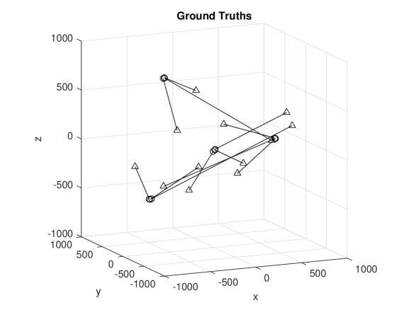
Figure 1: Ground truths in 3D space

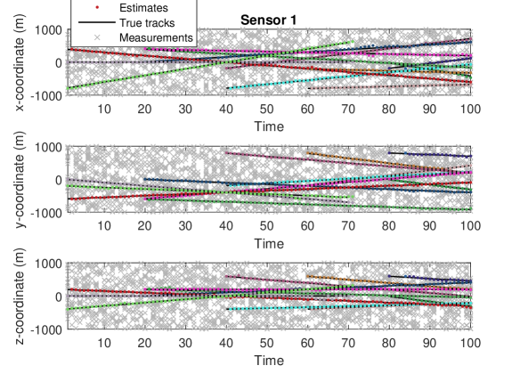
Figure 2: Sensor 1 measurements in $x,y,z$ coordinates versus time, also showing true tracks and filter estimates

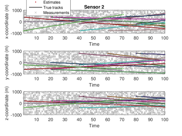
Figure 3: Sensor 2 measurements in $x,y,z$ coordinates versus time, also showing true tracks and filter estimates

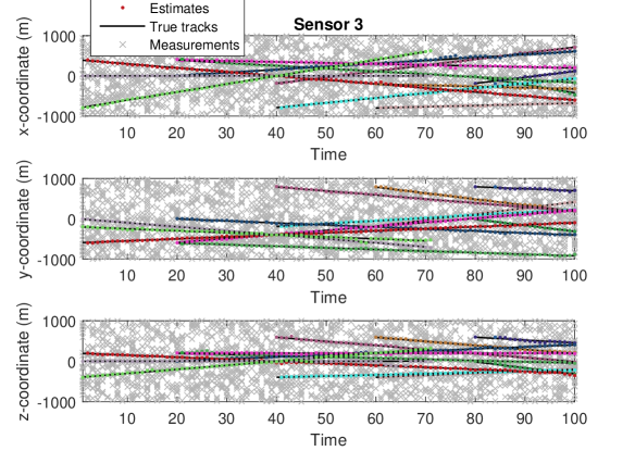
Figure 4: Sensor 3 measurements in $x,y,z$ coordinates versus time, also showing true tracks and filter estimates

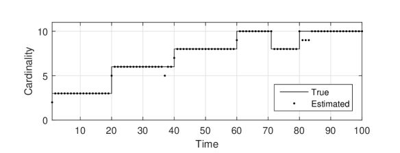
Figure 5: True and estimated cardinality versus time

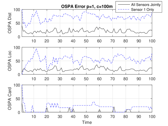
Figure 6: OSPA error with localization and cardinality components (p=1, c=100m)

The multi-sensor GLMB filter is implemented via the proposed Gibbs sampling technique. The filter is run with 10000 components and the Gibbs sampler is tempered by taking the $3$rd root of the cost tensor corresponding to a total of 3 sensors. Figure 1 shows the ground truths in 3D space. Figures 2, 3, 4 respectively show the measurements for sensors 1, 2, 3, in $x,y,z$ coordinates versus time, along with the ground truths and filter estimates also superimposed on the same figures. Note that the truths and estimates are the same for all sensors and are repeated on all sensor figures for convenience. Figure 5 shows the true and estimated cardinality versus time and Figure 6 shows the OSPA error ($p=1$ and $c=100m$) for the single and multiple sensor GLMB filters. It can be seen that for the multi-sensor GLMB filter all tracks are initiated and terminated correctly and the positions estimates are mostly accurate. This assessment is confirmed by the OSPA error which has a localization component consistent with the measurement noise and peaks in the cardinality component corresponding to times of target births and deaths.

V Efficient Implementation

V-A Memory vs Computation

The input to the Gibbs sampler (Algorithm 1) consists of  $P(1+\mathop{\textstyle\prod}\nolimits_{s=1}^{S}(1+M^{(s)}))$ entries for $\eta_{n}(j^{(1)},...,j^{(S)})$, $n=1,...,P$, and $(j^{(1)},...,j^{(S)})\in\{-1\}^{S}\uplus\{0:M^{(1)}\}\times...\times\{0:M^{(S)}\}$ (see (25)). For each $n$, the entries $\eta_{n}(j^{(1)},...,j^{(S)})$, $(j^{(1)},...,j^{(S)})\in\{-1\}^{S}\uplus\{0:M^{(1)}\}\times...\times\{0:M^{(S)}\}$ are used to construct a categorical distribution $\pi_{n}(j^{(1)},...,j^{(S)})$ with $1+\mathop{\textstyle\prod}\nolimits_{s=1}^{S}(1+M^{(s)})$ categories by

$$\pi_{n}(j^{(1)},...,j^{(S)})=K_{n}^{-1}\tilde{\eta}_{n}(j^{(1)},...,j^{(S)})$$ (34)

where

$$\tilde{\eta}_{n}(j^{(1)},...,j^{(S)}) = \eta_{n}(j^{(1)},...,j^{(S)})\mathop{\displaystyle\prod}\limits_{s=1}^{S}\mathop{\displaystyle\prod}\limits_{i\in\bar{n}}\left(1-1_{\{1:M^{(s)}\}}(j^{(s)})\delta_{j^{(s)}}[\gamma_{i}^{(s)}]\right)$$

$$K_{n} = \sum_{j^{(1)},...,j^{(S)}}\tilde{\eta}_{n}(j^{(1)},...,j^{(S)})$$

(see Proposition 2). The memory required for the categorical distribution is thus of order $\mathcal{O}(\mathop{\textstyle\prod}\nolimits_{s=1}^{S}M^{(s)})$.

If we factorize

$$\pi_{n}(j^{(1)},...,j^{(S)}) = \pi_{n}^{(S)}(j^{(S)}|j^{(S-1)},...,j^{(1)})...\pi_{n}^{(2)}(j^{(2)}|j^{(1)})\pi_{n}^{(1)}(j^{(1)})$$ (35)

$$= \mathop{\displaystyle\prod}\limits_{s=1}^{S}\pi_{n}^{(s)}(j^{(s)}|j^{(1)},...,j^{(s-1)})$$

$$= K_{n}^{-1}\mathop{\displaystyle\prod}\limits_{s=1}^{S}\tilde{\eta}_{n}^{(s)}(j^{(s)}|j^{(1)},...,j^{(s-1)})$$

then sampling $(j^{(1)},...,j^{(S)})$ from $\pi_{n}$ is equivalent to $j^{(1)}\sim\pi_{n}^{(1)}$, $j^{(2)}\sim$ $\pi_{n}^{(2)}(\cdot|j^{(1)})$, …., $j^{(S)}\sim\pi_{n}^{(S)}(\cdot|j^{(S-1)},...,j^{(1)})$. Hence instead of storing $1+\mathop{\textstyle\prod}\nolimits_{s=1}^{S}(1+M^{(s)})$ categories, we only require $2+\max_{s}M^{(s)}$ categories.

To determine the conditionals $\tilde{\eta}_{n}^{(s)}(j^{(s)}|j^{(1)},...,j^{(s-1)})$ we first specify some abbreviations. A Gaussian with mean $m$ and covariance $P$ is denoted by $\mathcal{N}(\cdot;m,P)$. Given $(m$,$P)$, the Kalman updated mean-covariance pair with measurement $j^{(s)}$ from sensor $s$, is denoted by $(m^{(s)}(j^{(s)}),P^{(s)}(j^{(s)}))$, i.e.

$$\mathcal{N}(y;m,P)\mathcal{N}(z_{j^{(s)}}^{(s)};H^{(s)}y,R^{(s)}) = \mathcal{N}(y;m^{(s)}(j^{(s)}),P^{(s)}(j^{(s)}))q^{(s)}(j^{(s)})$$

$$q^{(s)}(j^{(s)}) \triangleq \mathcal{N}(z_{j^{(s)}}^{(s)};H^{(s)}m,H^{(s)}PH^{(s)\text{T}}+R^{(s)})$$

Suppose $(m^{(s)}(j^{(s)}),P^{(s)}(j^{(s)}))$ is further updated with measurement $j^{(s)}$ from sensor $s$, then we denote the updated mean-covariance pair by $(m^{(s,t)}(j^{(s)},j^{(t)}),P^{(s,t)}(j^{(s)},j^{(t)}))$, i.e.

$$\mathcal{N}\!(y;m^{(s)}(j^{(s)}),P^{(s)}(j^{(s)}))\mathcal{N}(z_{j^{(t)}}^{(t)};H^{(t)}y,R^{(t)})\!\! = \!\!\mathcal{N}\!(y;m^{(s,t)}(j^{(s)}\!,j^{(t)}),P^{(s,t)}(j^{(s)}\!,j^{(t)}))q^{(s,t)}(j^{(s)}\!,j^{(t)})$$

$$q^{(s,t)}(j^{(s)},j^{(t)})\!\! = \!\!\mathcal{N}\!(z_{j^{(t)}}^{(t)};H^{(t)}m^{(s)}(j^{(s)}),H^{(t)}P^{(s)}(j^{(s)})H^{(t)\text{T}}+R^{(t)})$$

Further, given any $\mathcal{N}\left(y;m^{(\zeta,\ell_{n})},P^{(\zeta,\ell_{n})}\right)$ and $\psi_{\!Z_{+}^{(s)}\!}^{(s,j^{(s)})}(y,\ell_{n})$ we define

$$(\bar{m}^{(\zeta,\ell_{n},s)}(j^{(s)}),\bar{P}^{(\zeta,\ell_{n},s)}(j^{(s)})) \triangleq \left\{\begin{array}[]{cc}(m^{(\zeta,\ell_{n})},P^{(\zeta,\ell_{n})}),&j^{(s)}=0\\ (m^{(\zeta,\ell_{n},s)}(j^{(s)}),P^{(\zeta,\ell_{n},s)}),&j^{(s)}>0\end{array}\right.$$ (38)

$$\bar{q}^{(\zeta,\ell_{n},s)}(j^{(s)}) \triangleq \left\{\begin{array}[]{cc}1-P_{\!D}^{(s)}(\ell_{n}),&j^{(s)}=0\\ q^{(\zeta,\ell_{n},s)}(j^{(s)})P_{\!D}^{(s)}(\ell_{n})/\kappa^{(s)}(z_{j^{(s)}}^{(s)}),&j^{(s)}>0\end{array}\right.$$ (41)

so that

$$\mathcal{N}(y;m^{(\zeta,\ell_{n})},P^{(\zeta,\ell_{n})})\psi_{\!Z_{+}^{(s)}\!}^{(s,j^{(s)})}(y,\ell_{n})=\mathcal{N}(y;\bar{m}^{(\zeta,\ell_{n},s)}(j^{(s)}),\bar{P}^{(\zeta,\ell_{n},s)}(j^{(s)}))\bar{q}^{(\zeta,\ell_{n},s)}(j^{(s)})$$ (42)

Similarly we define $\bar{m}^{(\zeta,\ell_{n},1,...,t)}(j^{(1)}\!,...,j^{(t)})$, $\bar{P}^{(\zeta,\ell_{n},1,...,t)}(j^{(1)}\!,...,j^{(t)})$, and $\bar{q}^{(\zeta,\ell_{n},1,...,t)}(j^{(1)}\!,...,j^{(t)})$ so that

$$\!\!\!\!\!\!\!\!\!\!\!\!\!\!\!\!\!\!\!\!\!\!\!\!\!\!\!\!\!\mathcal{N}(y;\bar{m}^{(\zeta,\ell_{n},1,...,t-1)}(j^{(1)},...,j^{(t-1)}),\bar{P}^{(\zeta,\ell_{n},1,...,t-1)}(j^{(1)},...,j^{(t-1)}))\psi_{\!Z_{+}^{(t)}\!}^{(t,j^{(t)})}(y,\ell_{n})$$ (43)

$$= \mathcal{N}(y;\bar{m}^{(\zeta,\ell_{n},1,...,t)}(j^{(1)},...,j^{(t)}),\bar{P}^{(\zeta,\ell_{n},1,...,t)}(j^{(1)},...,j^{(t)}))\bar{q}^{(\xi,\ell_{n},1,...,t)}(j^{(1)},...,j^{(t)})$$ (44)

Note that the term $\bar{\psi}_{Z_{+_{\!}}}^{(\xi,j^{(1)},...,j^{(t)})\!}(\ell_{i\!})$ in $\eta_{n}(j^{(1)},...,j^{(t)})$ can be written as

$$\bar{\psi}_{Z_{+_{\!}}}^{(\xi,j^{(1)},...,j^{(t)})\!}(\ell_{n\!})=\int\bar{p}_{+}^{(\xi)}(y,\ell_{n})\prod\limits_{s=1}^{t}\psi_{\!Z_{+}^{(s)}\!}^{(s,j^{(s)})}(y,\ell_{n})dy.$$ (45)

by substituting the definition of $\psi_{\!Z_{+}\!}^{(j^{(1)},...,j^{(t)})}(\cdot,\ell_{n})$ into (26). Since $\bar{p}_{+}^{(\xi)}(y,\ell_{n})$ is a Gaussian, say $\bar{p}_{+}^{(\xi)}(y,\ell_{n})=\mathcal{N}\left(y;m^{(\xi,\ell_{n})},P^{(\xi,\ell_{n})}\right)$, we have

$$\bar{\psi}_{Z_{+_{\!}}}^{(\xi,j^{(1)},...,j^{(t)})\!}(\ell_{n\!}) = \int\mathcal{N}\left(y;m^{(\xi,\ell_{n})},P^{(\xi,\ell_{n})}\right)\prod\limits_{s=1}^{t}\psi_{\!Z_{+}^{(s)}\!}^{(s,j^{(s)})}(y,\ell_{n})dy$$

$$= \int\mathcal{N}\left(y;m^{(\xi,\ell_{n})},P^{(\xi,\ell_{n})}\right)\psi_{\!Z_{+}^{(1)}\!}^{(1,j^{(1)})}(y,\ell_{n})\prod\limits_{s=2}^{t}\psi_{\!Z_{+}^{(s)}\!}^{(s,j^{(s)})}(y,\ell_{n})dy$$

$$= \bar{q}^{(\xi,\ell_{n},1)}\left(j^{(1)}\right)\int\mathcal{N}\left(y;\bar{m}^{(\xi,\ell_{n},1)}(j^{(1)}),\bar{P}^{(\xi,\ell_{n},1)}(j^{(1)})\right)\prod\limits_{s=2}^{t}\psi_{\!Z_{+}^{(s)}\!}^{(s,j^{(s)})}(y,\ell_{n})dy$$

Consequently, iterating we have

$$\bar{\psi}_{Z_{+_{\!}}}^{(\xi,j^{(1)},...,j^{(t)})\!}(\ell_{n\!}) = \bar{q}^{(\xi,\ell_{n},1)}(j^{(1)})\int\mathcal{N}(y;\bar{m}^{(\xi,\ell_{n},1)}(j^{(1)}),\bar{P}^{(\xi,\ell_{n},1)})\prod\limits_{s=2}^{t}\psi_{\!Z_{+}^{(s)}\!}^{(s,j^{(s)})}(y,\ell_{n})dy$$ (46)

$$= \bar{q}^{(\xi,\ell_{n},1)}(j^{(1)})\bar{q}^{(\xi,\ell_{n},1,2)}(j^{(1)},j^{(2)})\times$$

$$\int\mathcal{N}(y;\bar{m}^{(\xi,\ell_{n},1,2)}(j^{(1)},j^{(2)}),\bar{P}^{(\xi,\ell_{n},1,2)}(j^{(1)},j^{(2)}))\prod\limits_{s=3}^{t}\psi_{\!Z_{+}^{(s)}\!}^{(s,j^{(s)})}(y,\ell_{n})dy$$

$$\vdots$$

$$= \bar{q}^{(\xi,\ell_{n},1)}(j^{(1)})\bar{q}^{(\xi,\ell_{n},1,2)}(j^{(1)},j^{(2)})...\bar{q}^{(\xi,\ell_{n},1,...,t)}(j^{(1)},...,j^{(t)})\times$$

$$\int\mathcal{N}(y;\bar{m}^{(\xi,\ell_{n},1,2,...t)}(j^{(1)},...,j^{(t)}),\bar{P}^{(\xi,\ell_{n},1,...,t)}(j^{(1)},...,j^{(t)}))dy$$

$$= \bar{q}^{(\xi,\ell_{n},1)}(j^{(1)})\bar{q}^{(\xi,\ell_{n},1,2)}(j^{(1)},j^{(2)})...\bar{q}^{(\xi,\ell_{n},1,...,t)}(j^{(1)},...,j^{(t)})$$

Equation (25) (reproduced here for convenience)

$$\eta_{n}(j^{(1)},...,j^{(t)})=\begin{cases}1-\bar{P}_{S}^{(\xi)\!}(\ell_{n}),&\!1\leq n\leq R,\text{ }(j^{(1)},...,j^{(t)})\!\prec 0\!,\\ \bar{P}_{S\!}^{(\xi)\!}(\ell_{n})\bar{\psi}_{Z_{+_{\!}}}^{(\xi,j^{(1)},...,j^{(t)})\!}(\ell_{n\!}),&\!1\leq n\leq R,\text{ }(j^{(1)},...,j^{(t)})\!\succeq 0,\\ 1-r_{B\!,+}(\ell_{n}),&\!R\!+\!1\leq n\leq P,\text{ }(j^{(1)},...,j^{(t)})\!\prec 0,\\ r_{B\!,+}(\ell_{n})\bar{\psi}_{Z_{+_{\!}}}^{(\xi,j^{(1)},...,j^{(t)})\!}(\ell_{n}),&\!R\!+\!1\leq n\leq P,\text{ }(j^{(1)},...,j^{(t)})\!\succeq 0.\end{cases}$$

can be written as a product of the factors

$$\eta_{n}(j^{(1)})=\begin{cases}1-\bar{P}_{S}^{(\xi)\!}(\ell_{n}),&\!1\leq n\leq R,\text{ }j^{(1)}=-1,\\ \bar{P}_{S\!}^{(\xi)\!}(\ell_{n})\bar{q}^{(\xi,\ell_{n},1)}(j^{(1)}),&\!1\leq n\leq R,\text{ }j^{(1)}\geq 0,\\ 1-r_{B\!,+}(\ell_{n}),&\!R\!+\!1\leq n\leq P,\text{ }j^{(1)}=-1,\\ r_{B\!,+}(\ell_{n})\bar{q}^{(\xi,\ell_{n},1)}(j^{(1)}),&\!R\!+\!1\leq n\leq P,\text{ }j^{(1)}\geq 0.\end{cases}$$ (47)

and for $t=2,...,S$

$$\eta_{n}(j^{(t)}|j^{(1)},...,j^{(t-1)})=\left\{\begin{array}[]{cc}1,&j^{(t)}=j^{(t-1)}=...=j^{(1)}=-1,\\ \bar{q}^{(\xi,\ell_{n},1,2,...,t)}(j^{(1)},...,j^{(t)}),&j^{(1)},...,j^{(t)}\geq 0,\\ 0,&\text{otherwise}\end{array}\right.$$

It can be seen from the above equations that the factors $\tilde{\eta}_{n}^{(1)}(\cdot),$ $\tilde{\eta}_{n}^{(2)}(\cdot|j^{(1)})$,…., $\tilde{\eta}_{n}^{(S)}(\cdot|j^{(S-1)},...,j^{(1)})$ can be computed on-the-fly. However, the corresponding probability distributions $\pi_{n}^{(1)}(\cdot)$, $\pi_{n}^{(2)}(\cdot|j^{(1)})$,…, $\pi_{n}^{(S)}(\cdot|j^{(S-1)},...,j^{(1)})$ involve the normalizing constants:

$$K_{n}^{(1)}(j^{(1)}) \triangleq \sum_{j^{(2)},...,j^{(S)}}\mathop{\displaystyle\prod}\limits_{s=2}^{S}\tilde{\eta}_{n}^{(s)}(j^{(s)}|j^{(1)},...,j^{(s-1)})$$

$$\vdots$$

$$K_{n}^{(1,...,t)}(j^{(1)},...,j^{(t)}) \triangleq \sum_{j^{(t+1)},...,j^{(S)}}\mathop{\displaystyle\prod}\limits_{s=t+1}^{S}\tilde{\eta}_{n}^{(s)}(j^{(s)}|j^{(1)},...,j^{(s-1)})$$

$$\vdots$$

$$K_{n}^{(1,...,S-1)}(j^{(1)},...,j^{(S-1)}) \triangleq \sum_{j^{(S)}}\tilde{\eta}_{n}^{(S)}(j^{(S)}|j^{(1)},...,j^{(S-1)})$$ (50)

since

$$\pi_{n}^{(1)}(j^{(1)}) = \sum_{j^{(2)},...,j^{(S)}}\pi_{n}(j^{(1)},...,j^{(S)})=\frac{1}{K_{n}}\sum_{j^{(2)},...,j^{(S)}}\mathop{\displaystyle\prod}\limits_{s=1}^{S}\tilde{\eta}_{n}^{(s)}(j^{(s)}|j^{(1)},...,j^{(s-1)})$$ (51)

$$= \frac{1}{K_{n}}\tilde{\eta}_{n}^{(1)}(j^{(1)})\sum_{j^{(2)},...,j^{(S)}}\mathop{\displaystyle\prod}\limits_{s=2}^{S}\tilde{\eta}_{n}^{(s)}(j^{(s)}|j^{(1)},...,j^{(s-1)})$$

$$= \tilde{\eta}_{n}^{(1)}(j^{(1)})\frac{K_{n}^{(1)}(j^{(1)})}{K_{n}}$$

and

$$\pi_{n}^{(t)}(j^{(t)}|j^{(1)},...,j^{(t-1)}) = \frac{\pi_{n}(j^{(1)},...,j^{(t-1)},j^{(t)})}{\pi_{n}(j^{(1)},...,j^{(t-1)})}=\frac{\sum\limits_{j^{(t+1)},...,j^{(S)}}\pi_{n}(j^{(1)},...,j^{(S)})}{\sum\limits_{j^{(t)},...,j^{(S)}}\pi_{n}(j^{(1)},...,j^{(S)})}$$

$$= \frac{\prod\limits_{s=1}^{t}\tilde{\eta}_{n}^{(s)}(j^{(s)}|j^{(1)},...,j^{(s-1)})\sum\limits_{j^{(t+1)},...,j^{(S)}}\prod\limits_{s=t+1}^{S}\tilde{\eta}_{n}^{(s)}(j^{(s)}|j^{(1)},...,j^{(s-1)})}{\prod\limits_{s=1}^{t-1}\tilde{\eta}_{n}^{(s)}(j^{(s)}|j^{(1)},...,j^{(s-1)})\sum\limits_{j^{(t)},...,j^{(S)}}\prod\limits_{s=t}^{S}\tilde{\eta}_{n}^{(s)}(j^{(s)}|j^{(1)},...,j^{(s-1)})}$$

$$= \tilde{\eta}_{n}^{(t)}(j^{(t)}|j^{(1)},...,j^{(t-1)})\frac{K_{n}^{(1,...,t)}(j^{(1)},...,j^{(t)})}{K_{n}^{(1,...,t-1)}(j^{(1)},...,j^{(t-1)})}$$

$$\vdots$$

$$\pi_{n}^{(S)}(j^{(S)}|j^{(1)},...,j^{(S-1)}) = \tilde{\eta}_{n}^{(S)}(j^{(S)}|j^{(1)},...,j^{(S-1)})\frac{1}{K_{n}^{(1,...,S-1)}(j^{(1)},...,j^{(S-1)})}$$ (53)

The complexity of computing the normalizing constants are still of order $\mathcal{O}(\mathop{\textstyle\prod}\nolimits_{s=1}^{S}M^{(s)})$. Note that computing these recursively as follows

$$K_{n}^{(1,...,S-2)}(j^{(1)},...,j^{(S-2)}) = \sum_{j^{(S-1)}}\tilde{\eta}_{n}^{(S-1)}(j^{(S-1)}|j^{(1)},...,j^{(S-2)})\sum_{j^{(S)}}\tilde{\eta}_{n}^{(S)}(j^{(S)}|j^{(1)},...,j^{(S-1)})$$

$$= \sum_{j^{(S-1)}}\tilde{\eta}_{n}^{(S-1)}(j^{(S-1)}|j^{(1)},...,j^{(S-2)})K_{n}^{(1,...,S-1)}(j^{(1)},...,j^{(S-1)})$$

$$\vdots$$

$$K_{n}^{(1,...,t)}(j^{(1)},...,j^{(t)}) = \sum_{j^{(t+1)}}\tilde{\eta}_{n}^{(t+1)}(j^{(t+1)}|j^{(1)},...,j^{(t)})\sum_{j^{(t)},...,j^{(S)}}\mathop{\displaystyle\prod}\limits_{s=t}^{S}\tilde{\eta}_{n}^{(s)}(j^{(s)}|j^{(1)},...,j^{(s-1)})$$

$$= \sum_{j^{(t+1)}}\tilde{\eta}_{n}^{(t+1)}(j^{(t+1)}|j^{(1)},...,j^{(t)})K_{n}^{(1,...,t+1)}(j^{(1)},...,j^{(t+1)})$$

$$\vdots$$

$$K_{n}^{(1)}(j^{(1)}) = \sum_{j^{(2)}}\tilde{\eta}_{n}^{(2)}(j^{(2)}|j^{(1)})\sum_{j^{(3)},...,j^{(S)}}\mathop{\displaystyle\prod}\limits_{s=3}^{S}\tilde{\eta}_{n}^{(s)}(j^{(s)}|j^{(1)},...,j^{(s-1)})$$ (56)

$$= \sum_{j^{(2)}}\tilde{\eta}_{n}^{(2)}(j^{(2)}|j^{(1)})K_{n}^{(1,2)}(j^{(1)},j^{(2)})$$

saves repeated computations but still incurs an $\mathcal{O}(\mathop{\textstyle\prod}\nolimits_{s=1}^{S}M^{(s)})$ complexity.

It is possible to replace sampling from the categorical distribution $\tilde{\eta}_{n}(\cdot|\gamma_{1:n-1}^{\prime},\gamma_{n+1:P})$ in the (block) Gibbs sampler by a single iteration of the Metropolis-Hastings algorithm with target distribution $\tilde{\eta}_{n}(\cdot|\gamma_{1:n-1}^{\prime},\gamma_{n+1:P})$. Other alternatives include adaptive rejection sampling (ARS) [58], adaptive rejection Metropolis sampling [59], and others such as [60]. While such approach avoids the $\mathcal{O}(\mathop{\textstyle\prod}\nolimits_{s=1}^{S}M^{(s)})$ complexity, the Gibbs sampler may take longer to converge.

V-B Alternative Target Distribution

Note that (22) is not the only choice of distribution that ensures valid components with high weights are chosen more often than those with low weights. Instead of sampling from $\pi(I_{+},\theta_{+}|I,\xi)\propto\omega_{Z_{{}_{\!}+}}^{(I,\xi,I_{+},\theta_{+})}$, this subsection introduces an alternative target distribution for the Gibbs sampler, which can drastically reduce the complexity. Unique samples from the alternative target distribution are then reweighted according to (32).

Suppose that we choose a target distribution of the form $1_{{\Gamma}}(\gamma)\prod\nolimits_{n=1\!}^{P}\eta_{n}(\gamma_{n})$, where each $\eta_{n}$ has the Markov property, i.e. $\eta_{n}^{(s)}(j^{(s)}|j^{(1)},...,j^{(s-1)})=\eta_{n}^{(s)}(j^{(s)}|j^{(s-1)})$. Then $\tilde{\eta}_{n}^{(s)}(j^{(s)}|j^{(1)},...,j^{(s-1)})$ = $\tilde{\eta}_{n}^{(s)}(j^{(s)}|j^{(s-1)})$, i.e.

$$\tilde{\eta}_{n}^{(s)}(j^{(1)},...,j^{(S)})=\mathop{\displaystyle\prod}\limits_{s=1}^{S}\tilde{\eta}_{n}^{(s)}(j^{(s)}|j^{(s-1)}).$$

and consequently, each normalizing constant reduces to a function of only a single index as follows

$$K_{n}^{(1,...,S-1)}(j^{(1)},...,j^{(S-1)}) = \sum_{j^{(S)}}\tilde{\eta}_{n}^{(S)}(j^{(S)}|j^{(S-1)})\triangleq K_{n}^{(S-1)}(j^{(S-1)})$$ (57)

$$K_{n}^{(1,...,S-2)}(j^{(1)},...,j^{(S-2)}) = \sum_{j^{(S-1)}}\tilde{\eta}_{n}^{(S-1)}(j^{(S-1)}|j^{(S-2)})K_{n}^{(S-1)}(j^{(S-1)})\triangleq K_{n}^{(S-2)}(j^{(S-2)})$$

$$\vdots$$

$$K_{n}^{(1,...,t)}(j^{(1)},...,j^{(t)}) = \sum_{j^{(t+1)}}\tilde{\eta}_{n}^{(t+1)}(j^{(t+1)}|j^{(t)})K_{n}^{(t+1)}(j^{(t+1)})\triangleq K_{n}^{(t)}(j^{(t)})$$

$$\vdots$$

$$K_{n}^{(1)}(j^{(1)}) = \sum_{j^{(2)}}\tilde{\eta}_{n}^{(2)}(j^{(2)}|j^{(1)})K_{n}^{(2)}(j^{(2)})$$ (60)

Since we only need to compute $2+M^{(S-1)}$ of the $K_{n}^{(S-1)}(j^{(S-1)})$, …., $2+M^{(t)}$ of the $K_{n}^{(t)}(j^{(t)})$,…, $2+M^{(1)}$ of the $K_{n}^{(1)}(j^{(1)})$, the complexity is of order $\mathcal{O}(\mathop{\textstyle\sum}\nolimits_{s=1}^{S}M^{(s)})$, a drastic reduction from $\mathcal{O}(\mathop{\textstyle\prod}\nolimits_{s=1}^{S}M^{(s)})$.

To ensure $\tilde{\eta}_{n}^{(s)}(j^{(1)},...,j^{(S)})$ is well-defined on $\{-1\}^{S}\uplus\{0:M^{(1)}\}\times...\times\{0:M^{(S)}\}$, we require the Markov transition kernel $\tilde{\eta}_{n}^{(s)}(\cdot|j^{(\cdot s-1)})$ to satisfy

$$\tilde{\eta}_{n}^{(s)}(j^{(s)}|-1) = \delta_{-1}[j^{(s)}]$$ (61)

$$\tilde{\eta}_{n}^{(s)}(-1|j^{(s-1)}) = \delta_{j^{(s-1)}}[-1]$$ (62)

for each $s>1$. In other words, if the chain starts with -1 then each subsequent state is -1, and if the chain doesn’t start with -1 then each subsequent state cannot take on -1. This implies $K_{n}^{(s)}(-1)=\sum_{j^{(s+1)}}\tilde{\eta}_{n}^{(s+1)}(j^{(s+1)}|-1)=\tilde{\eta}_{n}^{(s+1)}(-1|-1)=1$, and hence

$$K_{n}^{(S-1)}(j^{(S-1)}) = \left\{\begin{array}[]{cc}1,&j^{(S-1)}=-1\\ \sum\limits_{j^{(S)}=0}^{M^{(S)}}\tilde{\eta}_{n}^{(S)}(j^{(S)}|j^{(S-1)}),&j^{(S-1)}>-1\end{array}\right.$$ (65)

$$K_{n}^{(s)}(j^{(s)}) = \left\{\begin{array}[]{cc}1,&j^{(s)}=-1\\ \sum\limits_{j^{(s+1)}=0}^{M^{(s+1)}}\tilde{\eta}_{n}^{(s+1)}(j^{(s+1)}|j^{(s)})K_{n}^{(s+1)}(j^{(s+1)}),&j^{(s)}>-1\end{array}\right.$$ (68)

For $j^{(s)},j^{(s-1)}>-1$, a possible choice of $\eta_{n}^{(s)}(j^{(s)}|j^{(s-1)})$ is one that is independent of $j^{(s-1)}$, i.e. $\eta_{n}^{(s)}(j^{(s)})\triangleq\bar{q}^{(\xi,\ell_{n},s)}\left(j^{(s)}\right)$, which yields

$$K_{n}^{(s)}(j^{(s)})=\left\{\begin{array}[]{cc}1,&j^{(s)}=-1\\ \Upsilon_{n}^{(s)}\Upsilon_{n}^{(s+1)}...\Upsilon_{n}^{(S-1)}&j^{(s)}>-1\end{array}\right.$$ (69)

where

$$\Upsilon_{n}^{(s)} \triangleq \sum_{j^{(s+1)}=0}^{M^{(s+1)}}\tilde{\eta}_{n}^{(s+1)}(j^{(s+1)})$$ (70)

$$\tilde{\eta}_{n}^{(s)}(j^{(s)}) \triangleq \eta_{n}^{(s)}(j^{(s)})\mathop{\displaystyle\prod}\limits_{i\in\bar{n}}\left(1-1_{\{1:M^{(s)}\}}(j^{(s)})\delta_{j^{(s)}}[\gamma_{i}^{(s)}]\right)$$ (71)

Hence, the conditional distributions for the Gibbs sampler are

$$\pi_{n}^{(1)}(j^{(1)}) = \tilde{\eta}_{n}^{(1)}(j^{(1)})\frac{K_{n}^{(1)}(j^{(1)})}{K_{n}}$$ (72)

$$= \frac{1}{K_{n}}\left\{\begin{array}[]{cc}\tilde{\eta}_{n}^{(1)}(-1),&j^{(1)}=-1\\ \tilde{\eta}_{n}^{(1)}(j^{(1)})\Upsilon_{n}^{(1)}\Upsilon_{n}^{(2)}...\Upsilon_{n}^{(S-1)},&j^{(1)}>-1\end{array}\right.$$

$$\vdots$$

$$\pi_{n}^{(t)}(j^{(t)}|j^{(t-1)}) = \tilde{\eta}_{n}^{(t)}(j^{(t)}|j^{(t-1)})\frac{K_{n}^{(t)}(j^{(t)})}{K_{n}^{(t-1)}(j^{(t-1)})}$$ (76)

$$= \frac{1}{K_{n}^{(t-1)}(j^{(t-1)})}\left\{\begin{array}[]{cc}1,&j^{(t)}=j^{(t-1)}=-1\\ \tilde{\eta}_{n}^{(t)}(j^{(t)})\Upsilon_{n}^{(t)}...\Upsilon_{n}^{(S-1)},&j^{(t)}>,j^{(t-1)}>-1\end{array}\right.$$

$$\vdots$$

$$\pi_{n}^{(S)}(j^{(S)}|j^{(S-1)}) = \tilde{\eta}_{n}^{(S)}(j^{(S)}|j^{(S-1)})\frac{1}{K_{n}^{(S-1)}(j^{(S-1)})}$$ (80)

$$= \frac{1}{K_{n}^{(S-1)}(j^{(S-1)})}\left\{\begin{array}[]{cc}1,&j^{(S)}=j^{(S-1)}=-1\\ \tilde{\eta}_{n}^{(S)}(j^{(S)}),&j^{(S)},j^{(S-1)}>-1\end{array}\right.$$ (83)

The alternative target distribution can be interpreted as an approximation of the original target distribution. When $(j^{(1)},...,j^{(S)})\succeq-1$,

$$\bar{\psi}_{Z_{+_{\!}}}^{(\xi,j^{(1)},...,j^{(t)})\!}(\ell_{n\!})=\bar{q}^{(\xi,\ell_{n},1)}\left(j^{(1)}\right)\bar{q}^{(\xi,\ell_{n},1,2)}\left(j^{(1)},j^{(2)}\right)...\bar{q}^{(\xi,\ell_{n},1,2,...,t)}\left(j^{(1)},...,j^{(t)}\right)$$

can be treated as the joint association probability of the measurements $z_{j^{(1)}}^{(1)},...,z_{j^{(t)}}^{(t)}$ to track $\ell_{n}$ given the history $\xi$. Also each $\bar{q}^{(\zeta,\ell_{n},s)}\left(j^{(s)}\right)$ can be interpreted as the association probability of measurements $z_{j^{(s)}}^{(s)}$ to track $\ell_{i\!}$given the history $\xi$. In choosing $\eta_{n}^{(s)}(j^{(s)}|j^{(s-1)})=\bar{q}^{(\xi,\ell_{n},s)}\left(j^{(s)}\right)$, we are making the simplifying assumption that the association of measurement $z_{j^{(s)}}^{(s)}$, from sensor $s$, to track $\ell_{n\!}$ is independent of associations of measurements from other sensors (to track $\ell_{n}$). Consequently, the joint association probability of the measurements $z_{j^{(1)}}^{(1)},...,z_{j^{(S)}}^{(S)}$, to track $\ell_{n}$, is given by the product of the association probabilities $\bar{q}^{(\xi,\ell_{n},s)}\left(j^{(s)}\right)$. Intuitively, if the the product of the association probabilities $\bar{q}^{(\xi,\ell_{n},s)}\left(j^{(s)}\right)$ is high/low, then the joint association probability of the measurements $z_{j^{(1)}}^{(1)},...,z_{j^{(S)}}^{(S)}$ is also high/low.

Remark: If $\bar{\psi}_{Z_{+_{\!}}}^{(\xi,j^{(1)},...,j^{(t)})\!}(\ell_{n\!})$, is positive, then the product of the association probabilities $\bar{q}^{(\xi,\ell_{n},s)}\left(j^{(s)}\right)$ is also positive, i.e. the support of the alternative target distribution contains the support of the original target distribution. To see this note from (45) that $\bar{\psi}_{Z_{+_{\!}}}^{(\xi,j^{(1)},...,j^{(t)})\!}(\ell_{n\!})$ is actually independent of the order of the sensors even though we computed it using sensor 1, then sensor 2 and so on. Further suppose that there exists an $s$ such that $\bar{q}^{(\xi,\ell_{n},s)}\left(j^{(s)}\right)=0$. Since $\bar{\psi}_{Z_{+_{\!}}}^{(\xi,j^{(1)},...,j^{(t)})\!}(\ell_{n\!})$ is independent of the order of the sensors, computing it starting from sensor $s$, yields $\bar{\psi}_{Z_{+_{\!}}}^{(\xi,j^{(1)},...,j^{(t)})\!}(\ell_{n\!})=0$.

A more expensive alternative choice is $\eta_{n}^{(s)}(j^{(s)}|j^{(s-1)})=\bar{q}^{(\xi,\ell_{n},s-1,s)}\left(j^{(s-1)},j^{(s)}\right)$. The additional computation comes from the calculation of normalizing constants (68) rather than (69). On the other hand, this choice of $\eta_{n}^{(s)}(j^{(s)}|j^{(s-1)})$ yields a better approximation of $\eta_{n}^{(s)}(j^{(1)},...,j^{(S)})$. However, since the weights for the components will be corrected after the Gibbs sampling step, the advantage of a better approximation is not substantial.

VI Conclusions

This paper proposed an efficient implementation of the Multi-sensor GLMB filter by integrating the prediction and update into one step along with an efficient algorithm for truncating the GLMB filtering density based on Gibbs sampling. The resulting algorithm is an on-line multi-sensor multi-object tracker with linear complexity in the number of measurements of each sensor and quadratic in the number of hypothesized tracks. This implementation is also applicable to approximations such as the labeled multi-Bernoulli (LMB) filter since this filter requires a special case of the GLMB prediction and a full GLMB update to be performed [37].

References

• [1] Y. Bar-Shalom and T. E. Fortmann, Tracking and Data Association.   San Diego: Academic Press, 1988.
• [2] S. S. Blackman and R. Popoli, Design and Analysis of Modern Tracking Systems, ser. Artech House radar library.   Artech House, 1999.
• [3] R. Mahler, Statistical Multisource-Multitarget Information Fusion.   Artech House, 2007.
• [4] R. Mahler, Advances in Statistical Multisource-Multitarget Information Fusion,    Artech House, 2014.
• [5] R. Mahler, “Multitarget Bayes filtering via first-order multitarget moments,” IEEE Trans. Aerosp. Electron. Syst., vol. 39, no. 4, pp. 1152–1178, 2003.
• [6] R. Mahler, “PHD filters of higher order in target number,” IEEE Trans. Aerosp. Electron. Syst., vol. 43, no. 4, pp. 1523–1543, 2007.
• [7] B.-T. Vo, B.-N. Vo, and A. Cantoni, “The cardinality balanced Multi-Target Multi-Bernoulli filter and its implementations,” IEEE Trans. Signal Process., vol. 57, no. 2, pp. 409–423, 2009.
• [8] B.-N. Vo, B. T. Vo, N.-T. Pham, and D. Suter, “Joint detection and estimation of multiple objects from image observations,” IEEE Trans. Signal Process., vol. 58, no. 10, pp. 5129–5141, 2010.
• [9] M. Tobias and A. D. Lanterman, “Probability hypothesis density-based multitarget tracking with bistatic range and doppler observations,” IEE Proc. - Radar, Sonar & Navigation, vol. 152, no. 3, pp. 195–205, 2005.
• [10] D. E. Clark and J. Bell, “Bayesian multiple target tracking in forward scan sonar images using the PHD filter,” IEE Proc. - Radar, Sonar & Navigation, vol. 152, no. 5, pp. 327–334, 2005.
• [11] E. Maggio, M. Taj, and A. Cavallaro, “Efficient multitarget visual tracking using random finite sets,” IEEE Trans. Circuits Syst. Video Technol., vol. 18, no. 8, pp. 1016–1027, 2008.
• [12] R. Hoseinnezhad, B.-N. Vo, B. T. Vo, and D. Suter, “Visual tracking of numerous targets via multi-bernoulli filtering of image data,” Pattern Recognition, vol. 45, no. 10, pp. 3625–3635, 2012.
• [13] R. Hoseinnezhad, B.-N. Vo, and B.-T. Vo, “Visual tracking in background subtracted image sequences via multi-bernoulli filtering,” IEEE Trans. Signal Process., vol. 61, no. 2, pp. 392–397, 2013.
• [14] S. Rezatofighi, S. Gould, B. -T. Vo, B.-N. Vo, K. Mele, and R. Hartley, “Multi-target tracking with time-varying clutter rate and detection profile: Application to time-lapse cell microscopy sequences,” IEEE Trans. Med. Imag., vol. 34, no. 6, pp. 1336–1348, 2015.
• [15] J. Mullane, B.-N. Vo, M. Adams, and B.-T. Vo, “A random-finite-set approach to Bayesian SLAM,” IEEE Trans. Robot., vol. 27, no. 2, pp. 268–282, 2011.
• [16] C. Lundquist, L. Hammarstrand, and F. Gustafsson, “Road intensity based mapping using radar measurements with a Probability Hypothesis Density filter,” IEEE Trans. Signal Process., vol. 59, no. 4, pp. 1397–1408, 2011.
• [17] C. S. Lee, D. Clark, and J. Salvi, “SLAM with dynamic targets via single-cluster PHD filtering,” IEEE J. Sel. Topics Signal Process., vol. 7, no. 3, pp. 543–552, 2013.
• [18] G. Battistelli, L. Chisci, S. Morrocchi, F. Papi, A. Benavoli, A. Di Lallo, A. Farina, and A. Graziano, “Traffic intensity estimation via PHD filtering,” Proc. 2008 European Radar Conf. (EuRAD), pp. 340–343, Oct. 2008.
• [19] D. Meissner, S. Reuter, and K. Dietmayer, “Road user tracking at intersections using a multiple-model PHD filter,” Proc. 2013 IEEE Intelligent Vehicles Symposium, pp. 377–382, June 2013.
• [20] B. Ristic, B.-N. Vo, and D. Clark, “A note on the reward function for PHD filters with sensor control,” IEEE Trans. Aerosp. Electron. Syst., vol. 47, no. 2, pp. 1521–1529, 2011.
• [21] H. G. Hoang and B. T. Vo, “Sensor management for multi-target tracking via multi-Bernoulli filtering,” Automatica, vol. 50, no. 4, pp. 1135–1142, 2014.
• [22] A. Gostar, R. Hoseinnezhad, and A. Bab-Hadiashar, “Robust multi-bernoulli sensor selection for multi-target tracking in sensor networks,” IEEE Signal Process. Lett., vol. 20, no. 12, pp. 1167–1170, 2013.
• [23] H. Hoang, , B.-N. Vo, B.-T., Vo, and R. Mahler, “The Cauchy-Schwarz divergence for Poisson point processes,” IEEE Trans. Inf. Theory, vol. 61, no. 8, pp. 4475- 4485, 2015.
• [24] A.K. Gostar, R. Hoseinnezhad, and A. Bab-Hadiashar, “Multi-Bernoulli sensor control using Cauchy-Schwarz divergence,” Proc. 19th  Int. Conf. Inf. Fusion, pp. 651-657, 2016.
• [25] A.K. Gostar, R. Hoseinnezhad, and A. Bab-Hadiashar, “Multi-Bernoulli sensor-selection for multi-target tracking with unknown clutter and detection profiles,” Signal Processing, vol. 119, pp. 28-42, 2016.
• [26] A.K. Gostar, R. Hoseinnezhad, and A. Bab-Hadiashar, “Multi-bernoulli sensor control via minimization of expected estimation errors,” IEEE Trans. Aerosp. Electron. Syst., (to appear) 2017.
• [27] X. Zhang, “Adaptive control and reconfiguration of mobile wireless sensor networks for dynamic multi-target tracking,” IEEE Trans. Autom. Control, vol. 56, no. 10, pp. 2429–2444, 2011.
• [28] G. Battistelli, L. Chisci, C. Fantacci, A. Farina, and A. Graziano, “Consensus CPHD filter for distributed multitarget tracking,” IEEE J. Sel. Topics Signal Process., vol. 7, no. 3, pp. 508–520, 2013.
• [29] M. Uney, D. Clark, and S. Julier, “Distributed fusion of PHD filters via exponential mixture densities,” IEEE J. Sel. Topics Signal Process., vol. 7, no. 3, pp. 521–531, 2013.
• [30] A.-A. Saucan, M. Coates and M. Rabbat, “Multi-sensor multi-Bernoulli filter,” Available: https://arxiv.org/pdf/1609.05108.pdf
• [31] B.-N. Vo, S.S. Singh, W.K. Ma, “Tracking multiple speakers using random sets,” in Proc. Int. Conf. Acoustic Speech & Sig. Proc., vol. 2, pp. 357-360, 2004.
• [32] B.-T. Vo and B.-N. Vo, “Labeled random finite sets and multi-object conjugate priors,” IEEE Trans. Signal Process., vol. 61, no. 13, pp. 3460–3475, 2013.
• [33] B.-N. Vo, B.-T. Vo, and D. Phung, “Labeled random finite sets and the Bayes multi-target tracking filter,” IEEE Trans. Signal Process., vol. 62, no. 24, pp. 6554–6567, 2014.
• [34] B.-N. Vo, B.-T. Vo, and H. Hoang, “An Efficient Implementation of the Generalized Labeled Multi-Bernoulli Filter,” IEEE Trans. Signal Process.,  vol. 65, no. 8, pp. 1975–1987, 2017. Available: https://arxiv.org/abs/1606.08350.
• [35] F. Papi, B.-N. Vo, B.-T. Vo, C. Fantacci, and M. Beard, “Generalized labeled multi-Bernoulli approximation of multi-object densities,” IEEE Trans. Signal Process., vol. 63, no. 20, pp. 5487-5497, 2015.
• [36] M. Beard, B.-T. Vo, B.-N. Vo, and S. Arulampalam “Void probabilities and cauchy-schwarz divergence for generalized labeled multi-bernoulli models,” arXiv preprint arXiv:1510.05532, 2015. Available: https://arxiv.org/pdf/1510.05532.pdf.
• [37] S. Reuter, B.-T. Vo, B.-N. Vo, and K. Dietmayer, “The labeled multi-Bernoulli filter,” IEEE Trans. Signal Process., vol. 62, no. 12, pp. 3246–3260, 2014.
• [38] C. Fantacci, and F. Papi, “Scalable multisensor multitarget tracking using the marginalized-GLMB density,” IEEE Signal Process. Lett. vol. 23, no. 6, pp. 863-867, 2016.
• [39] M. Beard, B.-T. Vo, and B.-N. Vo, “Bayesian multi-target tracking with merged measurements using labelled random finite sets,” IEEE Trans. Signal Process., vol. 63, no. 6, pp. 1433-1447, 2015.
• [40] M. Beard, S. Reuter, K. Granström, B.-T. Vo, B.-N. Vo, and A. Scheel, “Multiple extended target tracking with labeled random finite sets,” IEEE Trans. Signal Process., vol. 64, no. 7, pp. 1638- 1653, 2016.
• [41] Y. Punchihewa, B.-N. Vo, and B.-T. Vo, “A Generalized Labeled Multi-Bernoulli Filter for Maneuvering Targets,” Proc. 19th  Int. Conf. Inf. Fusion, pp. 980-986. July 2016. Available: https://arxiv.org/pdf/1603.04565.pdf
• [42] M Jiang, W Yi, R Hoseinnezhad, L Kong, “Adaptive Vo-Vo filter for maneuvering targets with time-varying dynamics,” Proc. 19th  Int. Conf. Inf. Fusion, pp. 666-672. July 2016.
• [43] F. Papi and D. Y. Kim, “A particle multi-target tracker for superpositional measurements using labeled random finite sets,” IEEE Trans. Signal Process. vol. 63, no. 16, pp. 4348-4358, 2015.
• [44] D.Y. Kim, B.-T. Vo, and B.-N. Vo, “Data fusion in 3D vision using a RGB-D data via switching observation model and its application to people tracking, ”. Proc. Int. Conf. Control, Aut. & Inf. Sciences, pp. 91-96, 2013..
• [45] Y. Punchihewa, F. Papi, and R. Hoseinnezhad. “Multiple target tracking in video data using labeled random finite set.” Proc. Int. Conf. Control, Aut. & Inf. Sciences, pp. 13-18, 2014.
• [46] T Rathnayake, AK Gostar, R Hoseinnezhad, A Bab-Hadiashar, “Labeled multi-Bernoulli track-before-detect for multi-target tracking in video,” Proc. 8  Int. Conf. Inf. Fusion, pp. 1353-1358, 2015.
• [47] D.Y. Kim, B.-N. Vo, and B.-T. Vo, “Online Visual Multi-Object Tracking via Labeled Random Finite Set Filtering,” arXiv preprint arXiv:1611.06011, 2016.
• [48] A.K. Gostar, R. Hoseinnezhad, and A. Bab-Hadiashar, “Sensor control for multi-object tracking using labeled multi-Bernoulli filter,” Proc. 17th  Int. Conf. Inf. Fusion, pp. 1-8. July 2014.
• [49] H. Deusch, S. Reuter, and K. Dietmayer, “The labeled multi-Bernoulli SLAM filter,” IEEE Signal Process. Lett., vol. 22, no. 10, pp.1561-1565, 2015.
• [50] C. Fantacci, B-N. Vo, B-T. Vo, G. Battistelli, and L. Chisci, “Consensus labeled random finite set filtering for distributed multi-object tracking,” arXiv preprint arXiv:1501.01579 (2015).
• [51] B.S. Wei, B. Nener, W.F. Liu; and M. Liang, “Centralized Multi-Sensor Multi-Target Tracking with Labeled Random Finite Sets,” Proc. Int. Conf. Control, Aut. & Inf. Sciences, 2016.
• [52] B.-N. Vo, S. Singh, and A. Doucet, “Sequential Monte Carlo methods for multi-target filtering with random finite sets,” IEEE Trans. Aerosp. Electron. Syst., vol. 41, no. 4, pp. 1224–1245, 2005.
• [53] S. Geman and D. Geman, “Stochastic relaxation, Gibbs distributions, and the Bayesian restoration of images,” IEEE Trans. Pattern Anal. Mach. Intell., vol. 6, no. 6, pp. 721–741, 1984.
• [54] G. Casella and E. I. George, “Explaining the Gibbs sampler,” The American Statistician, vol. 46, no. 3, pp. 167–174, 1992.
• [55] L. Devroye, Non-uniform random variate generation.   Springer-Verlag, 1986.
• [56] C. Geyer and E. Thompson, “Annealing Markov Chain Monte Carlo with applications to ancestral inference,” J. American Statistical Association, vol. 90, no. 431, pp. 909-920, Sep. 1995.
• [57] R. Neal, “Annealed importance sampling,” Statistics & Computing, vol. 11, pp. 125-139, 2000.
• [58] W.R. Gilks, and P. Wild, “Adaptive Rejection Sampling for Gibbs Sampling,” Journal of the Royal Statistical Society. Series C (Applied Statistics), vol. 41, no. 2, pp. 337–348, 1992.
• [59] W.R. Gilks, N.G. Best, and K.K.C Tan, “Adaptive Rejection Metropolis Sampling within Gibbs Sampling,” Journal of the Royal Statistical Society. Series C (Applied Statistics), vol. 44 , no. 4, pp. 455–472, 1995.
• [60] C. Ritter, M.A. Tanner, “Facilitating the Gibbs Sampler: The Gibbs Stopper and the Griddy-Gibbs Sampler,” Journal of the American Statistical Association, vol. 87, no. 419, pp. 861–868, 1992.
• [61] D. Schumacher, B.-T. Vo, and B.-N. Vo, “A consistent metric for performance evaluation of multi-object filters,” IEEE Trans. Signal Process., vol. 56, no. 8, pp. 3447–3457, 2008.