Analytic approach to magneto-strain tuning of electronic transport through a graphene nanobubble: Perspectives for a strain sensor

Abstract

We consider the scattering of Dirac particles in graphene due to the superposition of an external magnetic field and mechanical strain. As a model for a graphene nanobubble, we find exact analytical solutions for single-particle states inside and outside a circular region submitted to the fields. Finally, we obtain analytical expressions for the scattering cross-section, as well as for the Landauer current through the circular region. Our results provide a fully-analytical treatment for electronic transport through a graphene nanobubble, showing that a combination of a physical magnetic field and strain leads to valley polarization and filtering of the electronic current. Moreover, our analytical model provides an explicit metrology principle to measure strain by performing conductance experiments under a controlled magnetic field imposed over the sample.

I Introduction

Graphene is an allotrope of carbon in the form of an atomic monolayer, arranged as a honeycomb lattice with $C_{6v}=Z_{2}\otimes C_{3v}$ symmetry. It is then mathematically described as a superposition of two Bravais lattices with $C_{3v}$ symmetry, usually denoted as A and B sub lattices, respectively Wallace (1947); Geim (2011); Neto et al. (2009); Mu$\tilde{\text{n}}$oz (2016). As a consequence tight-binding, as well as ab-initio band structure calculations, show that the energy spectrum possesses linear dispersion in the vicinity of two non-equivalent, so called Dirac points (or valleys) in reciprocal space Geim (2011); Neto et al. (2009); Novoselov et al. (2005); Peres (2010). This particular feature allows for the description of graphene electronic properties in terms of an effective Dirac Hamiltonian, whose eigenstates are given by two-component spinors, where a pseudo-spin property emerges as a consequence of the two sub-latticesPeres (2010); Novoselov et al. (2005); Neto et al. (2009); Kim and Neto (2008); Mu$\tilde{\text{n}}$oz (2016). Those states exhibit pseudo-relativistic properties, such as relativistic Landau levels in the presence of an external magnetic field Goerbig (2011); Neto et al. (2009); Sarma et al. (2011), where the two Dirac points are connected by time-reversal symmetry, and hence the two valleys are degenerate Goerbig (2011). Perhaps an even more interesting feature arises under the presence of mechanical strain. Within the Dirac approximation, strain enters as a gauge field whose curl represents a pseudo-magnetic field that reverses sign at each Dirac point, thus breaking the valley symmetry Vozmediano et al. (2010); Guinea et al. (2010a, b); Low and Guinea (2010); Juan et al. (2013); Guinea et al. (2008); Pe$\tilde{\text{n}}$a and Mu$\tilde{\text{n}}$oz (2015); Amorim et al. (2016). Conductance experiments have shown the emergence of pseudo-relativistic Landau levels in the presence of strain solely, thus suggesting that the magnitude of the associated pseudo-magnetic fields can reach over 100 Tesla for a small nano-bubble Levy et al. (2010); Klimov et al. (2012) or ridge Yan et al. (2012) in graphene. From the theoretical perspective, strain-induced gauge fields have been incorporated into extended Dirac Hamiltonians that involve the simultaneous description of both non-equivalent Dirac cones Vozmediano et al. (2010); Juan et al. (2013, 2012); Gopalakrishnan et al. (2012); Pe$\tilde{\text{n}}$a and Mu$\tilde{\text{n}}$oz (2015); Amorim et al. (2016). Other physical effects, such as charge density waves, can also be included in the form of generalized SU(2) gauge fieldsGopalakrishnan et al. (2012).

Arbitrary strain patterns generate inhomogeneous pseudo-magnetic fields, and in an experimental sample it is difficult to characterize with nanometric resolution the precise geometry of a strain pattern in order to correlate it with the magnitude of the corresponding pseudo-magnetic field (see for instance Ref. Neek-Amal et al. (2013) for graphene under triaxial stress). Theoretical models to represent nanobubbles in graphene are mainly based on a gaussian approximation for the strain field, that leads to a non-uniform pseudo-magnetic field possessing a well defined compact support in the spatial domain Moldovan et al. (2013); Arias et al. (2015). On the other hand, experimental STEM measurements Levy et al. (2010); Klimov et al. (2012); Yan et al. (2012) are consistent with a nearly uniform pseudomagnetic field over a circular region with a radius commensurate to the size of the nanobubble Klimov et al. (2012) (15 - 25 nm typically), or the width of a ridge Yan et al. (2012). Ab-initio calculations support these experimental findings as well Zhu et al. (2015). Interesting perspectives to use this effect in nanoscale devices have been discussed, for instance by the construction of strain superlattices Pellegrino et al. (2012); Zhang et al. (2017).

On the other hand, electronic conductance is relatively straightforward to measure, and here we show that it can be directly correlated with the magnitude of the strain field imposed, thus providing a proof-of-principle for the development of a piezoelectric sensor with nanometric resolution. In what follows, we shall present a theoretical model to represent elastic scattering of conduction electrons through a graphene nano bubble, represented as a disk-shaped region submitted to mechanical strain and an external magnetic field normal to the plane, as depicted in Fig. 1. We shall obtain exact analytical solutions for the eigenstates within the region, as well as for the states scattered off the region. By calculating the differential and total scattering cross-sections, we obtain the transmission coefficient Tudorovskiy et al. (2012); Peres (2010) through the region, and calculate the Landauer conductance Peres (2010) for a given bias applied. Our analytical results show explicitly how a combination of a physical magnetic field and mechanical strain leads to valley-polarization and filtering of the current Low and Guinea (2010); Settnes et al. (2016).

II Model

Let us start by writing the effective Dirac Hamiltonian for graphene, involving both valleys $\mathbf{K}_{\pm}=\pm\frac{4\pi}{3\sqrt{3}a}\hat{\mathbf{e}}_{x}$, in the presence of generalized SU(2) gauge fields Gopalakrishnan et al. (2012)

$$\hat{H}=\hbar v_{F}\left[\Gamma_{x}\left(\hat{p}_{x}-\sum_{i=1}^{3}A_{x}^{i}Q_{i}\right)+\Gamma_{y}\left(\hat{p}_{y}-\sum_{i=1}^{3}A_{y}^{i}Q_{i}\right)\right].$$ (1)

Here the Fermi velocity $v_{F}\sim c/300\sim 10^{6}$ m/s. We have defined the matrices

$$\Gamma_{x} = \hat{\tau}_{3}\otimes\hat{\sigma}_{1},\,\,\,\,\Gamma_{y}=\hat{\tau}_{0}\otimes\hat{\sigma}_{2},$$

$$Q_{0} = \hat{\tau}_{0}\otimes\hat{\sigma}_{0},\,\,\,\,Q_{1}=-\hat{\tau}_{2}\otimes\hat{\sigma}_{2},$$

$$Q_{2} = \hat{\tau}_{1}\otimes\hat{\sigma}_{2},\,\,\,\,Q_{3}=\hat{\tau}_{3}\otimes\hat{\sigma}_{0},$$ (2)

where $\sigma$ and $\tau$ are the Pauli matrices acting on the sublattice and valley spaces respectively. The spinor structure over which the Hamiltonian operates is

$$\Psi=\left(\begin{array}[]{c}\psi_{A}^{+}\\ \psi_{B}^{+}\\ \psi_{A}^{-}\\ \psi_{B}^{-}\end{array}\right)\equiv\left(\begin{array}[]{c}\Psi^{(+)}\\ \Psi^{(-)}\end{array}\right).$$ (9)

To introduce the effect of an external magnetic field and mechanical strain, we chose the following gauge fields:

$$A_{x}^{0} = -y\frac{B_{0}}{2},\,\,\,A_{y}^{0}=x\frac{B_{0}}{2},\,\,\,A_{x}^{3}=-y\frac{B_{S}}{2},\,\,\,A_{y}^{3}=x\frac{B_{S}}{2},$$

$$A_{x}^{1} = A_{y}^{1}=A_{x}^{2}=A_{y}^{2}=0,$$ (10)

where $B_{0}$ represents the magnitude of the physical, external magnetic field, while $B_{S}$ characterizes the magnitude of the pseudo-magnetic field induced by mechanical strain. The $\mathbf{A}^{1}$ and $\mathbf{A}^{2}$ gauge fields, that may be used to model charge density waves Gopalakrishnan et al. (2012), are set to zero since these phenomena are not under consideration in our present analysis. For notational convenience, let us define the combination

$$B_{\xi}=B_{0}+\xi B_{S},$$ (11)

representing the effective magnetic field acting at each of the two non-equivalent Dirac cones centered at the wave-vectors $\bm{K}_{\xi}=\xi\frac{4\pi}{3\sqrt{3}a}\hat{\mathbf{e}}_{x}$, for $\xi=\pm$ respectively.

In this case, the Hamiltonian in Eq. (1) has the block diagonal form:

$$\hat{H}=\left(\begin{array}[]{cc}\hat{H}^{+}&0\\ 0&\hat{H}^{-}\end{array}\right),$$ (14)

where we have defined

$$\hat{H}^{\xi}= \xi\hbar v_{F}\left[\hat{\sigma}_{1}\left(\hat{p}_{x}+\frac{y}{2}B_{\xi}\right)+\xi\hat{\sigma}_{2}\left(\hat{p}_{y}-\frac{x}{2}B_{\xi}\right)\right].$$ (15)

A more symmetric, and hence more convenient representation of the Hamiltonian in Eq. (14) is obtained by transforming the spinor in Eq.(9) as follows

$$\Psi\rightarrow\tilde{\Psi}=\hat{S}\Psi=\left(\begin{array}[]{c}\psi_{A}^{+}\\ \psi_{B}^{+}\\ \psi_{B}^{-}\\ \psi_{A}^{-}\end{array}\right),$$ (20)

where we have defined the unitary transformation $\hat{S}=\hat{S}^{-1}$ by the matrix

$$\hat{S}=\left(\begin{array}[]{cc}\hat{\sigma}_{0}&0\\ 0&\hat{\sigma}_{1}\end{array}\right),$$ (23)

where $\hat{\sigma}_{0}$ is the $2\times 2$ identity matrix. The transformed Hamiltonian, after Eq. (14), is given by

$$\hat{H}\rightarrow\hat{H}_{S}=\hat{S}\hat{H}\hat{S}^{-1}=\left(\begin{array}[]{cc}\hat{H}^{+}&0\\ 0&\hat{\sigma}_{1}\hat{H}^{-}\hat{\sigma}_{1}\end{array}\right)\equiv\left(\begin{array}[]{cc}\hat{H}_{S}^{+}&0\\ 0&\hat{H}_{S}^{-}\end{array}\right).$$ (28)

In particular, making use of the identity $\hat{\sigma}_{1}\hat{\sigma}_{2}\hat{\sigma}_{1}=-\hat{\sigma}_{2}$, we have for the diagonal components of the transformed Hamiltonian

$$\hat{H}_{S}^{\xi}=\xi\hbar v_{F}\left[\hat{\sigma}_{1}\left(\hat{p}_{x}+\frac{y}{2}B_{\xi}\right)+\hat{\sigma}_{2}\left(\hat{p}_{y}-\frac{x}{2}B_{\xi}\right)\right].$$ (29)

In terms of the definitions above, we have the block-diagonal eigenvalue problem

$$\left(\begin{array}[]{cc}\hat{H}_{S}^{(+)}-E^{(+)}&0\\ 0&\hat{H}_{S}^{(-)}-E^{(-)}\end{array}\right)\left(\begin{array}[]{c}\tilde{\Psi}^{(+)}\\ \tilde{\Psi}^{(-)}\end{array}\right)=0,$$ (30)

that reduces to two independent eigenvalue problems for the block Hamiltonians $\hat{H}_{S}^{\pm}$ at each valley $\mathbf{K}_{\pm}$.

The eigenvalue problem was solved analytically, with further technical details presented in Appendix A. In particular, the energy eigenvalues for the extended Hamiltonian describing both cones under the presence of magnetic and strain fields are found to be

$$E_{\lambda}^{\xi}(n)=\lambda\hbar v_{F}\sqrt{2n|B_{\xi}|},\,\,\,\,n=0,1,\ldots$$ (31)

with $\lambda=\pm 1$ representing particle (hole) eigenstates, while $\xi=\pm$ being the valley index. The spinor eigenvectors, for $n>0$, are given by

$$\tilde{\Psi}_{n,m}^{\xi,\lambda}(r,\phi)=C_{m,n}^{\xi,\lambda}\left(\begin{array}[]{cc}z^{\frac{|m|}{2}}e^{-z/2}L_{n_{\rho}}^{|m|}(z)e^{im\phi}\\ i\,\alpha_{n}^{\xi}z^{\frac{|m+1|}{2}}e^{-z/2}L_{n^{\prime}_{\rho}}^{|m+1|}(z)e^{i(m+1)\phi}\end{array}\right)$$ (34)

where we have defined the dimensionless variable $z=|B_{\xi}|r^{2}/2$, and $L_{n}^{m}(z)$ are the associated Laguerre polynomials Gradshteyn and Ryshik (1965). The coefficients in Eq. (34) are defined, for $n>0$ by:

$$n_{\rho} = n-\theta(-B_{\xi})-\frac{|m|-m\,{\rm{{\rm sign}}}B_{\xi}}{2}$$

$$n^{\prime}_{\rho} = n_{\rho}-\theta(B_{\xi})+\theta(-m)$$

$$\alpha_{n}^{\xi} = \lambda\xi n^{\theta(-m)-1/2},$$ (35)

with $\theta(x)$ the Heaviside step function, and the normalization cefficients

$$C_{m,n}^{\xi,\lambda}= \left(\frac{|B_{\xi}|}{2\pi}\right)^{\frac{1}{2}}\left\{\frac{\Gamma(|m|+n_{\rho}+1)}{n_{\rho}!}+\left(\alpha_{n}^{\xi}\right)^{2}\frac{\Gamma(|m+1|+n^{\prime}_{\rho}+1)}{n_{\rho}^{{}^{\prime}}!}\right\}^{-1/2}.$$ (36)

The index $m$ is an integer, and $\Gamma(z)$ represents the Gamma function. For ${\rm sign}B_{\xi}=+1$, we have $-n\leq m<+\infty$, while for ${\rm sign}B_{\xi}=-1$ we have $-\infty<m\leq n-1$.

The state with $n=0$ is given, for ${\rm sign}B_{\xi}=+1$, with $m\geq 0$ by the expression

$$\tilde{\Psi}_{0,m\geq 0}^{\xi,\lambda}(r,\phi)=C_{m\geq 0,0}^{\xi,\lambda}\left(\begin{array}[]{c}z^{\frac{m}{2}}e^{-z/2}e^{im\phi}\\ 0\end{array}\right).$$ (37)

On the other hand, for ${\rm sign}B_{\xi}=-1$, the state $n=0$ with $m<0$ is given by

$$\tilde{\Psi}_{0,m<0}^{\xi,\lambda}(r,\phi)=C_{m<0,0}^{\xi,\lambda}\left(\begin{array}[]{c}0\\ z^{\frac{|m+1|}{2}}e^{-z/2}e^{i(m+1)\phi}\end{array}\right).$$ (38)

Here, the normalization coefficients are given by

$$C_{m,0}^{\xi,\lambda}= \left(\frac{|B_{\xi}|}{2\pi}\right)^{1/2}\left\{\theta(B_{\xi})\Gamma(|m|+1)+\theta(-B_{\xi})\Gamma(|m+1|+1)\right\}^{-1/2}.$$ (39)

III Scattering through a nanobuble with magnetic field and mechanical strain

Let us now consider the problem of transport through a graphene sheet submitted to a physical magnetic field and an induced pseudo-magnetic field due to mechanical strain. Experimentally, STEM measurements Levy et al. (2010); Klimov et al. (2012); Yan et al. (2012) reveal that when graphene is submitted to local strain patterns, the resulting pseudomagnetic fields possess a well defined compact support in the spatial domain. A number of attempts have been published in the literature to model such patterns by a gaussian distributed field, and the corresponding models for the associated Dirac single-particle eigenstates and energy eigenvalues can only be studied numerically Moldovan et al. (2013). More recently, Bahamon et al.Bahamon et al. (2015) studied the conductance induced by different strain nanobubles numerically using molecular dynamics and tight-binding simulations. However, STEM experiments reveal that the magnitude of the pseudomagnetic field due to local strain patterns is nearly uniform within a region with a characteristic radius on the order of $15-25$ nm Levy et al. (2010); Klimov et al. (2012); Yan et al. (2012); Zhu et al. (2015).

Based on the previous statements, we prefer to study the system within a realistic approximation that allows us to obtain analytical solutions. We thus assume that the fields are non-zero only within a circular region of radius $a\sim 15-25$ nm (see Fig.1). We consider then the problem of two-dimensional elastic scattering of an incident free spinor with momentum $\mathbf{k}=(k,0)$ and energy $E_{k,\lambda}^{\xi}=\lambda\hbar v_{F}|\mathbf{k}|$ ($v_{F}\sim 10^{6}$ m/s), with $\lambda=\pm 1$ the “band” index, and $\xi=\pm 1$ referring to each valley $\mathbf{K}_{\xi}$, respectively. We will give below a detailed description that generalizes the method in Ref.Adhikari (1986) to the case of Dirac fermions. Using this method we will be able to compute the differential scattering cross-section that will be used in the next section to compute the electronic transport.

We begin by considering a free spinor eigenstate incident from the left towards the circular scattering center. This spinor is given by the solution of Eq. (29) with $B_{\xi}=0$, and thus is given by:

$$\tilde{\Psi}_{in}^{(\lambda,\xi)}(r,\phi)=\frac{1}{\sqrt{2}}\left(\begin{array}[]{c}1\\ \lambda\xi\end{array}\right)e^{ikr\cos\phi}.$$ (40)

We now proceed with the standard partial wave analysis for scattering. Let us first consider the general solution for the problem in the absence of external fields and interactions. Following the procedure described in detail in Appendix A, we have that the spinor corresponding to the eigenvalue $\hbar m_{j}$ of the total angular momentum operator $\hat{J}_{3}=\hat{L}_{3}+\hat{\sigma}_{3}/2$ is of the form

$$\tilde{\Psi}_{m_{j}}(r,\phi)=r^{-1/2}\left(\begin{array}[]{c}f_{m_{j}}(r)e^{i(m_{j}-1/2)\phi}\\ -i\,g_{m_{j}}(r)e^{i(m_{j}+1/2)\phi}\end{array}\right).$$ (41)

The partial wave decomposition, i.e. the resolution into angular momentum channels $m_{j}$, of the Dirac equation then reduces to the effective coupled eigenvalue problem for the radial functions

$$\left(\begin{array}[]{cc}-\lambda\xi k&\hat{D}^{\dagger}\\ \hat{D}&-\lambda\xi k\end{array}\right)\left(\begin{array}[]{c}f_{m_{j}}\\ g_{m_{j}}\end{array}\right)=0,$$ (46)

where we have defined (see Appendix A) the differential operators $\hat{D}=\frac{d}{dr}-\frac{m_{j}}{r}$ and its adjoint $\hat{D}^{\dagger}=-\frac{d}{dr}-\frac{m_{j}}{r}$. Solving for the system Eq.(46), the radial components of the spinor are determined through the diagonal eigenvalue problem

$$\left(\begin{array}[]{cc}\hat{D}^{\dagger}\hat{D}-k^{2}&0\\ 0&\hat{D}\hat{D}^{\dagger}-k^{2}\end{array}\right)\left(\begin{array}[]{c}f_{m_{j}}\\ g_{m_{j}}\end{array}\right)=0.$$ (47)

The matrix Eq. (47) leads to the pair of differential equations

$$\left[-\frac{d^{2}}{dr^{2}}+\frac{(m_{j}-1/2)^{2}}{r^{2}}-k^{2}\right]f_{m_{j}}(r) =0,$$

$$\left[-\frac{d^{2}}{dr^{2}}+\frac{(m_{j}+1/2)^{2}}{r^{2}}-k^{2}\right]g_{m_{j}}(r) =0.$$ (48)

The general solution of the system in Eq.(48) is expressed in terms of Bessel functions of the first and second kind,

$$f_{m_{j}}(r)= c_{1}\sqrt{kr}J_{m_{j}-1/2}(kr)+c_{2}\sqrt{kr}Y_{m_{j}-1/2}(kr),$$

$$g_{m_{j}}(r)= c_{3}\sqrt{kr}J_{m_{j}+1/2}(kr)+c_{4}\sqrt{kr}Y_{m_{j}+1/2}(kr).$$ (49)

However, the Dirac equation in its first-order differential form Eq.(46) imposes a relation between the upper and lower components, i.e.

$$g_{m_{j}}(r) = \frac{\lambda\xi}{k}\hat{D}f_{m_{j}}(r)=-\lambda\xi\left[c_{1}\sqrt{kr}J_{m_{j}+1/2}(kr)+c_{2}\sqrt{kr}Y_{m_{j}+1/2}(kr)\right]$$ (50)

where we applied the Bessel function identity Gradshteyn and Ryshik (1965)

$$\frac{dZ_{\alpha}}{dx}-\frac{\alpha}{x}Z_{\alpha}(x)=-Z_{\alpha+1}(x).$$ (51)

The result in Eq.(50) clearly fixes $c_{3}=-c_{1}$ and $c_{4}=-c_{2}$ in Eq.(49).

III.1 Phase-shift

In elastic scattering theory, the phase shift captures the effect of a scattering region over the transmitted particle waves. In order to express the phase shift associated to the circular region depicted in Fig.1, let us first consider the asymptotic properties of the Bessel functions Gradshteyn and Ryshik (1965), for $kr\gg 1$,

$$J_{m}(kr) \sim\sqrt{\frac{2}{\pi kr}}\cos\left(kr-\left(m+\frac{1}{2}\right)\frac{\pi}{2}\right),$$

$$Y_{m}(kr) \sim\sqrt{\frac{2}{\pi kr}}\sin\left(kr-\left(m+\frac{1}{2}\right)\frac{\pi}{2}\right).$$ (52)

Taking these properties into account, we have that the asymptotic form for the general spinor solution Eq.(41) with angular momentum $m\equiv m_{j}-1/2$ is, for $kr\gg 1$

$$\tilde{\Psi}_{m_{j}}^{\lambda,\xi}(r,\phi)\sim\sqrt{\frac{2}{\pi kr}}\tilde{C}_{m}\left(\begin{array}[]{c}e^{im\phi}\cos\left(kr-\left(m+\frac{1}{2}\right)\frac{\pi}{2}+\delta_{m}\right)\\ i\lambda\xi\,e^{i(m+1)\phi}\cos\left(kr-\left(m+\frac{3}{2}\right)\frac{\pi}{2}+\delta_{m}\right)\end{array}\right).$$ (55)

Here, we have defined the global coefficients and phase shifts by

$$\tilde{C}_{m}= \sqrt{k}\sqrt{c_{1}^{2}+c_{2}^{2}},$$

$$\tan\delta_{m}= -c_{2}/c_{1}.$$ (56)

To determine the phase shift $\delta_{m}$ associated to each angular momentum channel $m$, we have to match each spinor component of the general solution Eq. (41), and its first derivative, to the corresponding solution inside the region submitted to the effective magnetic field $B_{\xi}$, at the boundary $r=a$. In particular, for the upper spinor component, we have the following system of equations:

$$c_{1}\sqrt{k}J_{m}(ka)+c_{2}\sqrt{k}Y_{m}(ka) =C_{m,n}^{\lambda,\xi}\left(\frac{|B_{\xi}|a^{2}}{2}\right)^{\frac{|m|}{2}}e^{-\frac{|B_{\xi}|a^{2}}{4}}L_{n_{\rho}}^{|m|}\left(\frac{|B_{\xi}|a^{2}}{2}\right)$$ (57)

$$c_{1}\,k^{3/2}J_{m}^{{}^{\prime}}(ka)+c_{2}\,k^{3/2}Y_{m}^{{}^{\prime}}(ka) =C_{m,n}^{\lambda,\xi}\left(\frac{|B_{\xi}|a^{2}}{2}\right)^{\frac{|m|}{2}}|B_{\xi}|ae^{-\frac{|B_{\xi}|a^{2}}{4}}\left\{\left(\frac{|m|}{|B_{\xi}|a^{2}}-\frac{1}{2}\right)L_{n_{\rho}}^{|m|}\left(\frac{|B_{\xi}|a^{2}}{2}\right)\right.$$

$$\left.\quad-L_{n_{\rho}-1}^{|m|+1}\left(\frac{|B_{\xi}|a^{2}}{2}\right)\right\}.$$ (58)

An exact analytical solution of this linear system yields a closed expression for the phase shift $\delta_{m}$,

$$\tan\delta_{m}=\frac{J_{m+1}(ka)+\displaystyle\frac{J_{m}(ka)}{ka}\left\{|m|-m-\frac{|B_{\xi}|a^{2}}{2}-\frac{L_{n_{\rho}-1}^{|m|+1}(|B_{\xi}|a^{2}/2)}{L_{n_{\rho}}^{|m|}(|B_{\xi}|a^{2}/2)}\right\}}{Y_{m+1}(ka)+\displaystyle\frac{Y_{m}(ka)}{ka}\left\{|m|-m-\frac{|B_{\xi}|a^{2}}{2}-\frac{L_{n_{\rho}-1}^{|m|+1}(|B_{\xi}|a^{2}/2)}{L_{n_{\rho}}^{|m|}(|B_{\xi}|a^{2}/2)}\right\}}.$$ (59)

Here, we have made use of the following the mathematical identities Gradshteyn and Ryshik (1965)

$$\frac{d}{dx}L_{n}^{|m|}(x) = -L_{n-1}^{|m|+1}(x),$$

$$\frac{d}{dx}J_{m}(x) = \frac{1}{2}\left(J_{m-1}(x)-J_{m+1}(x)\right),$$

$$\frac{d}{dx}Y_{m}(x) = \frac{1}{2}\left(Y_{m-1}(x)-Y_{m+1}(x)\right).$$ (60)

III.2 Scattering cross section

In the region $r\gg a$, the state will be given by a linear combination of the incident and scattered spinor

$$\tilde{\Psi}_{out}(r,\phi)\sim\frac{1}{\sqrt{2}}\left(\begin{array}[]{c}1\\ \lambda\xi\end{array}\right)e^{ikr\cos\phi}+\left(\begin{array}[]{c}f_{1}(\phi)\\ f_{2}(\phi)\end{array}\right)\frac{e^{ikr}}{\sqrt{r}},$$ (61)

with amplitudes $f_{1}(\phi)$ and $f_{2}(\phi)$ for each component of the scattered spinor. In the same region, we have that this expression must be equal to the asymptotic form of the solution, represented in terms of phase shifts, Eq.(55). In order to analyse the contribution of each partial wave with angular momentum $\hbar m$, we use the mathematical identity

$$e^{ikr\cos\phi} =\sum_{m=-\infty}^{\infty}i^{m}e^{im\phi}J_{m}(kr)\sim\sqrt{\frac{2}{\pi kr}}\sum_{m}i^{m}e^{im\phi}\cos\left(kr-\frac{\pi}{2}\left(m+\frac{1}{2}\right)\right)$$ (62)

Therefore, substituting into Eq.(61) we find that:

$$\tilde{\Psi}_{out}(r,\phi)= \sum_{m}\left(\begin{array}[]{c}\frac{i^{m}}{\sqrt{\pi kr}}e^{im\phi}\cos\left(kr-\frac{\pi}{2}\left(m+\frac{1}{2}\right)\right)\\ \lambda\xi\frac{i^{m+1}}{\sqrt{\pi kr}}e^{i{(m+1)}\phi}\cos\left(kr-\frac{\pi}{2}\left(m+\frac{3}{2}\right)\right)\end{array}\right)+\left(\begin{array}[]{c}f_{1}(\phi)\\ f_{2}(\phi)\end{array}\right)\frac{e^{ikr}}{\sqrt{r}}.$$ (67)

Equating expressions (55) and (67), we demand for the pre-factors of $e^{\pm ikr}$ to be the same on both sides, thus yielding the following system of equations

$$\sum_{m}\left(\begin{array}[]{c}\frac{i^{m}}{2\sqrt{\pi k}}e^{im\phi}e^{-i\pi(m+1/2)/2}\\ \lambda\xi\frac{i^{(m+1)}}{2\sqrt{\pi k}}e^{i(m+1)\phi}e^{-i\pi(m+3/2)/2}\end{array}\right)+\left(\begin{array}[]{c}f_{1}(\phi)\\ f_{2}(\phi)\end{array}\right) =\frac{1}{\sqrt{2\pi k}}\sum_{m}\tilde{C}_{m}\left(\begin{array}[]{c}e^{im\phi}e^{-i\pi(m+1/2)/2+i\delta_{m}}\\ \lambda\xi\,i\,e^{i(m+1)\phi}e^{-i\pi(m+3/2)/2+i\delta_{m}}\end{array}\right)$$ (74)

$$\sum_{m}\left(\begin{array}[]{c}\frac{i^{m}}{2\sqrt{\pi k}}e^{im\phi}e^{i\pi(m+1/2)/2}\\ \lambda\xi\frac{i^{m+1}}{2\sqrt{\pi k}}e^{i(m+1)\phi}e^{i\pi(m+3/2)/2}\end{array}\right) =\sum_{m}\frac{\tilde{C}_{m}}{\sqrt{2\pi k}}\left(\begin{array}[]{c}e^{im\phi}e^{i\pi(m+1/2)/2}e^{-i\delta_{m}}\\ \lambda\xi\,i\,e^{i(m+1)\phi}e^{i\pi(m+3/2)/2}e^{-i\delta_{m}}\end{array}\right).$$ (79)

Using orthogonality of the basis $\left\{e^{im\phi}\right\}$, we can compute $\tilde{C}_{m}$, which is thus given by:

$$\tilde{C}_{m}= \frac{i^{m}}{\sqrt{2}}e^{i\delta_{m}}.$$ (80)

Inserting the previous result into the system of equations Eq.(79), we solve for the scattering amplitudes:

$$\left(\begin{array}[]{c}f_{1}(\phi)\\ f_{2}(\phi)\end{array}\right)=\frac{e^{-i\pi/4}}{2\sqrt{\pi k}}\sum_{m}\left(\begin{array}[]{c}e^{im\phi}\\ \lambda\xi e^{i(m+1)\phi}\end{array}\right)\left(e^{2i\delta_{m}}-1\right).$$ (81)

The differential scattering cross-section is given by the modulus of the vector above,

$$\frac{d\sigma}{d\phi}=|f_{1}(\phi)|^{2}+|f_{2}(\phi)|^{2},$$ (82)

and the total scattering cross section (with dimensions of length instead of area) is then given by integrating over the scattering angle $\phi$ ($0\leq\phi\leq 2\pi$)

$$\sigma= \int_{0}^{2\pi}\left(|f_{1}(\phi)|^{2}+|f_{2}(\phi)|^{2}\right)d\phi$$

$$= \frac{4}{k}\sum_{m=-\infty}^{\infty}\sin^{2}\delta_{m}.$$ (83)

IV Transmission and Landauer ballistic current

Let us consider a graphene stripe, of width $W$ ($y$-direction), which is connected to two semi-infinite graphene contacts held at chemical potentials $\mu_{L}$ and $\mu_{R}$, respectively. As a model for a nanobubble, we shall assume that a circular region of radius $a$ is submitted to a perpendicular uniform magnetic field ($\hat{\mathbf{e}}_{3}\,B_{0}$) and to mechanical strain as well. Typical experimental values for the characteristic diameter of graphene bubbles are $a\sim 15-25nm$ Levy et al. (2010); Klimov et al. (2012); Yan et al. (2012); Zhu et al. (2015), while a graphene ribbon will have typical widths $W\sim 10\mu m$ . Therefore, under realistic experimental conditions $a/W\ll 1$, and hence any influence of the edges of the ribbon over the carrier dynamics at the nanobubble becomes negligible. Within the Landauer ballistic picture, the net current along the stripe ($x$-direction) is given by the net counterflow of the particle currents emitted from the left and right semi-infinite graphene contacts, respectively. Each contact is assumed to be in thermal equilibrium, with the Fermi-Dirac distributions $f(E-\mu_{L},T)\equiv f_{L}(E)$ and $f_{R}(E)\equiv f(E-\mu_{R},T)$, respectively. A pictorial description of the system is shown in Fig. 1.

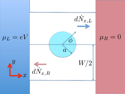
Figure 1: (Color online) Pictorial representation of the system. The left and right contacts are assumed as semi-infinite graphene regions, held at chemical potentials $\mu_{L}$ and $\mu_{R}$, respectively. The nano bubble is represented as a disk of radius $a$, submitted to the influence of the magnetic field and the mechanical strain.

The particle flux (per unit width) emitted by the left (L) and right (R) contacts, respectively, is defined as

$$dJ_{x,L/R}=v_{x}D_{L/R}(E)f_{L/R}(E)dE,$$ (84)

where $D_{L/R}(E)$ is the (surface-normalized) density of states at each contact.

The effect of the nanobubble over charge transport can be expressed as an effective one-dimensional cross-section $WT_{\xi}(E,\phi)$, with $T_{\xi}(E,\phi)$ the transmission coefficient in the direction specified by the angle $\phi$, for an incident spinor arising from the valley $\mathbf{K}_{\xi}$. We thus define the effective cross-section in the $\phi$-direction by the expression

$$W\,T_{\xi}(E_{k},\phi) =\frac{1}{\sigma(k)}\frac{d\sigma(k)}{d\phi}\sum_{n,\lambda}\delta\left(\lambda\,k-\frac{E_{n}^{\xi}}{\hbar v_{F}}\right)=\frac{\hbar v_{F}}{\sigma}\frac{d\sigma}{d\phi}\sum_{n,\lambda,\xi}\delta\left(E_{k,\lambda}-E_{n}^{\xi}\right)$$

$$=\frac{2\hbar^{2}v_{F}^{2}}{\sigma\pi}\sum_{m,m^{\prime},n,\lambda,\xi}\frac{1}{E_{k,\lambda}}e^{i(m-m^{\prime})\phi}e^{i(\delta_{m}-\delta_{m^{\prime}})}\sin\delta_{m}\sin\delta_{m^{\prime}}\delta\left(E_{k,\lambda}-E_{n}^{\xi}\right).$$ (85)

Here, the differential scattering cross-section is calculated from Eq.(82), while the total cross section is obtained in terms of the phase shifts by Eq.(83). The Dirac delta function enforces the energy conservation condition assumed for elastic scattering.

The particle flow (per unit time) along the $x$-direction emitted by the left (L) contact and arising from the $\mathbf{K}_{\xi}$ valley is ($v_{x}=v_{F}\cos\phi$)

$$d\dot{N}_{x,L}^{\xi}=W\,T_{\xi}(E,\phi)d\phi\,dJ_{x,L}=v_{F}\cos(\phi)\,D_{L}(E)\,f_{L}(E)dE\times W\,T_{\xi}(E,\phi)d\phi,$$

with an analogous expression for the right (R) particle flow. The net electric current flowing across the region will be $I=I_{+}+I_{-}$, with the valley-polarized component given by

$$I_{\xi}=e\int\left(d\dot{N}_{x,L}^{\xi}-d\dot{N}_{x,R}^{\xi}\right)=ev_{F}W\int_{-\infty}^{\infty}dE\left[D_{L}(E)f_{L}(E)-D_{R}(E)f_{R}(E)\right]\bar{T}_{\xi}(E).$$ (86)

Here, we have defined the net transmission coefficient for Dirac spinors at valley $\mathbf{K}_{\xi}$ as the angular average $\bar{T}_{\xi}(E)=\int_{-\pi/2}^{\pi/2}d\phi\,\cos\phi\,T_{\xi}(E,\phi)$, that reduces to the analytical expression

$$\bar{T}_{\xi}(E)=\frac{4\hbar^{2}v_{F}^{2}}{\pi W\,E\sigma}\sum_{n,p,m}\frac{(-1)^{p+1}}{4p^{2}-1}e^{i(\delta_{m}-\delta_{m-2p})}\left[\sin(\delta_{m})\sin(\delta_{m-2p})\,\delta\left(E-E_{n}^{\xi}\right)\right].$$ (87)

where we used the result

$$\int_{-\pi/2}^{\pi/2}d\phi\cos\phi\,e^{i(m-m^{\prime})\phi}=\delta_{m-m^{\prime},2p}\frac{2\,(-1)^{p+1}}{4p^{2}-1},\,\,\,p\in\mathbb{Z}.$$

It is important to remark that the valley-polarized transmission coefficients defined by Eq.(87) are not c-functions, but distributions (a superposition of Dirac-deltas), and hence it is not possible to plot them graphically. However, as will be discussed in detail later on in the context of the current-voltage characteristics, the transmission coefficient corresponding to the $\xi=(-)$ valley defines a denser distribution in energy space. The reason is that, for the effective pseudomagnetic field $B_{-}=B_{0}-B_{S}$ at this valley, the corresponding energy eigenvalues $E_{n}^{\xi}\sim\sqrt{|B_{\xi}|n}$ constitute a denser set than those of the $\xi=(+)$ valley, assuming for definiteness $B_{0}>0$ and $B_{S}>0$. Thus, as will be verified later, the valley-polarized current components should satisfy $I_{-}>I_{+}$. Assuming both contacts are identical semi-infinite graphene regions, the density of states are equal, and given by

$$D_{L}(E) = D_{R}(E)=D(E)=4\int\frac{d^{2}k}{(2\pi)^{2}}\left[\delta\left(E-\hbar v_{F}k\right)+\delta\left(E+\hbar v_{F}k\right)\right]=\frac{2}{\pi(\hbar v_{F})^{2}}\left[E\theta(E)+(-E)\theta(-E)\right]$$ (89)

$$= \frac{2|E|}{\pi(\hbar v_{F})^{2}}\theta(|E|),$$

where the factor of $4$ arises from the spin and valley degeneracy at each of the graphene semi-infinite contacts. With this consideration, the expression for the valley-polarized component of the current $I_{\xi}$ becomes

$$I_{\xi} =ev_{F}W\int_{-\infty}^{\infty}dED(E)\bar{T}_{\xi}(E)\left[f_{L}(E)-f_{R}(E)\right]$$

$$=\frac{8ev_{F}}{\pi^{2}}\sum_{n,m,p}\frac{(-1)^{p+1}}{\sigma(E_{n}^{\xi})(4p^{2}-1)}e^{i(\delta_{m}-\delta_{m-2p})}\sin\delta_{m}\sin\delta_{m-2p}\left[f_{L}(E_{n}^{\xi})-f_{R}(E_{n}^{\xi})\right],$$ (90)

with the total current given by $I=I_{+}+I_{-}$.

V Results and Discussion

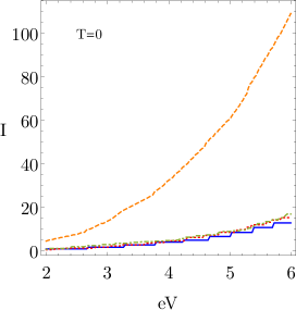
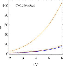
Figure 2: (Color online) Current (in units of $ev_{F}/a$) calculated from the analytical Eq.(90), as a function of applied bias $V$ (in units of $\hbar v_{F}/a$), for fixed $B_{0}a^{2}=1.8\tilde{\phi}_{0}$ and different values of $B_{S}$. The solid (blue) line corresponds to $B_{S}a^{2}=0$, the dotted (red) line corresponds to $B_{S}a^{2}=0.5\tilde{\phi}_{0}$, the dotdashed (green) line corresponds to $B_{S}a^{2}=1.1\tilde{\phi}_{0}$ and the dashed (orange) line corresponds to $B_{S}a^{2}=1.7\tilde{\phi}_{0}$, with $\tilde{\phi}_{0}\equiv(v_{F}/c)\hbar/e$. The subfigures (a), (b) and (c) correspond to the different values of the temperature, $T=0$, $T=0.02\,\hbar v_{F}/(k_{B}a)$ and $T=0.2\,\hbar v_{F}/(k_{B}a)$ respectively.

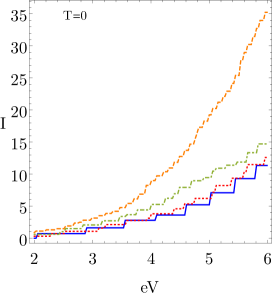
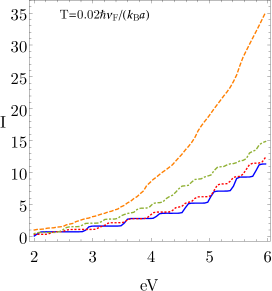
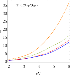
Figure 3: (Color online) Current (in units of $ev_{F}/a$) calculated from the analytical Eq.(90) , as a function of applied bias $eV$ (in units of $\hbar v_{F}/a$), for fixed $B_{0}a^{2}=2.1\tilde{\phi}_{0}$ and different values of $B_{S}$. The solid (blue) line corresponds to $B_{S}a^{2}=0$, the dotted (red) line corresponds to $B_{S}a^{2}=0.5\tilde{\phi}_{0}$, the dotdashed (green) line corresponds to $B_{S}a^{2}=1.1\tilde{\phi}_{0}$ and the dashed (orange) line corresponds to $B_{S}a^{2}=1.7\tilde{\phi}_{0}$, with $\tilde{\phi}_{0}\equiv(v_{F}/c)\hbar/e$. The subfigures (a), (b) and (c) correspond to the different values of the temperature, $T=0$, $T=0.02\,\hbar v_{F}/(k_{B}a)$ and $T=0.2\,\hbar v_{F}/(k_{B}a)$ respectively

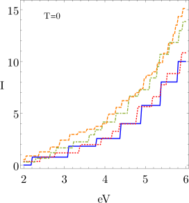
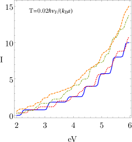
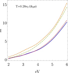
Figure 4: (Color online) Current (in units of $ev_{F}/a$) calculated from the analytical Eq.(90), as a function of applied bias $eV$ (in units of $\hbar v_{F}/a$), for fixed $B_{0}a^{2}=2.4\tilde{\phi}_{0}$ and different values of $B_{S}$. The solid (blue) line corresponds to $B_{S}a^{2}=0$, the dotted (red) line corresponds to $B_{S}a^{2}=0.5\tilde{\phi}_{0}$, the dotdashed (green) line corresponds to $B_{S}a^{2}=1.1\tilde{\phi}_{0}$ and the dashed (orange) line corresponds to $B_{S}a^{2}=1.7\tilde{\phi}_{0}$, with $\tilde{\phi}_{0}\equiv(v_{F}/c)\hbar/e$. The subfigures (a), (b) and (c) correspond to the different values of the temperature, $T=0$, $T=0.02\,\hbar v_{F}/(k_{B}a)$ and $T=0.2\,\hbar v_{F}/(k_{B}a)$ respectively.

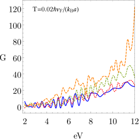
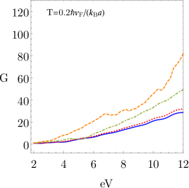
Figure 5: (Color online) Conductance (in units of $e^{2}/\hbar$) as a function of bias $eV$ (in units of $\hbar v_{F}/a$), calculated as the voltage-derivative of the analytical Eq.(90), for fixed $B_{0}a^{2}=2.1\tilde{\phi}_{0}$ and different values of $B_{S}$. The solid (blue) line corresponds to $B_{S}a^{2}=0$, the dotted (red) line corresponds to $B_{S}a^{2}=0.5\tilde{\phi}_{0}$, the dotdashed (green) line corresponds to $B_{S}a^{2}=1.1\tilde{\phi}_{0}$ and the dashed (orange) line corresponds to $B_{S}a^{2}=1.7\tilde{\phi}_{0}$, with $\tilde{\phi}_{0}\equiv(v_{F}/c)\hbar/e$. The subfigures (a) and (b) correspond to the different values of the temperature $T=0.02\,\hbar v_{F}/(k_{B}a)$ and $T=0.2\,\hbar v_{F}/(k_{B}a)$ respectively.

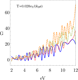
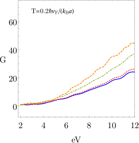
Figure 6: (Color online) Conductance (in units of $e^{2}/\hbar$) as a function of bias $eV$ (in units of $\hbar v_{F}/a$), calculated as the voltage-derivative of the analytical Eq.(90), for fixed $B_{0}a^{2}=2.4\tilde{\phi}_{0}$ and different values of $B_{S}$. The solid (blue) line corresponds to $B_{S}a^{2}=0$, the dotted (red) line corresponds to $B_{S}a^{2}=0.5\tilde{\phi}_{0}$, the dotdashed (green) line corresponds to $B_{S}a^{2}=1.1\tilde{\phi}_{0}$ and the dashed (orange) line corresponds to $B_{S}a^{2}=1.7\tilde{\phi}_{0}$, with $\tilde{\phi}_{0}\equiv(v_{F}/c)\hbar/e$. The subfigures (a) and (b) correspond to the different values of the temperature $T=0.02\,\hbar v_{F}/(k_{B}a)$ and $T=0.2\,\hbar v_{F}/(k_{B}a)$ respectively.

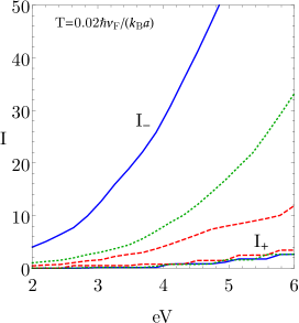
Figure 7: (Color online) The valley-polarized components of the current (in units of $ev_{F}/a$), calculated from the analytical Eq.(90), are displayed as a function of the applied bias $eV$ (in units of $\hbar v_{F}/a$), at finite temperature $T=0.02\,\hbar v_{F}/(k_{B}a)$, fixed $B_{0}a^{2}=2.1\tilde{\phi}_{0}$ and different values of $B_{S}$. The solid (blue) lines correspond to $B_{S}a^{2}=2\tilde{\phi}_{0}$, the dotted (green) lines correspond to $B_{S}a^{2}=1.7\tilde{\phi}_{0}$ and the dashed (red) lines correspond to $B_{S}a^{2}=1.1\tilde{\phi}_{0}$, with $\tilde{\phi}_{0}\equiv\hbar v_{F}/e$. The total current is $I=I_{+}+I_{-}$. A clear filtering effect in favour of the $I_{-}$ component versus the $I_{+}$ component is observed.

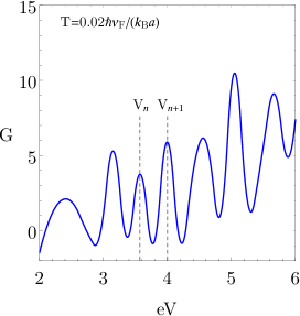
Figure 8: (Color online) Conductance (in units of $e^{2}/\hbar$) as a function of bias $eV$ (in units of $\hbar v_{F}/a$), calculated as the voltage-derivative of the analytical Eq.(90), for fixed $B_{0}a^{2}=2.1\tilde{\phi}_{0}$ and $B_{S}a^{2}=0.5\tilde{\phi}_{0}$ at a temperature $T=0.02\,\hbar v_{F}/(k_{B}a)$

In this section, we represent graphically the total current $I=I_{+}+I_{-}$ (in units of $ev_{F}/a$) calculated from the analytical formula Eq. (90) for the valley-polarized components $I_{\xi}$, both at zero and at finite temperatures (Figs. 2 - 4), for the particular choice of contact chemical potentials $\mu_{L}=eV$ and $\mu_{R}=0$. In Fig.2(a) we represent the total current for $T=0$, as a function of the applied bias voltage $V$, for a fixed value of the external magnetic field $B_{0}a^{2}=1.8\tilde{\phi}_{0}$, with $\tilde{\phi}_{0}\equiv(v_{F}/c)\frac{\hbar}{e}$. The different curves display the dependence of the current on the magnitude of the strain-induced pseudo-magnetic field $B_{S}$. Interestingly, there is a strong dependence of the current-voltage characteristics on the applied strain over the scattering region. One can also appreciate the staired shape of the curve, a feature that is more manifest at lower values of strain. This effect follows directly from the condition of elastic scattering (see Eq.(85)), since in order for the incident particle to be transmitted across the scattering region, its incident energy must be resonant to one of the eigenstates in the circular region submitted to the fields. The quasi-continuum distribution of energy values in the reservoirs allows for this condition be always fulfilled, for an interval within the window imposed by the external bias voltage. Moreover, let us notice that for contact chemical potentials $\mu_{L}=\alpha eV$ and $\mu_{R}=-\beta eV$, with $\alpha+\beta=1$ such that the net potential difference between the contacts is $V$, in the $T\rightarrow 0$ limit the difference between the two Fermi distributions in Eq.(90) becomes $f_{L}(E_{n}^{\xi})-f_{R}(E_{n}^{\xi})\rightarrow\Theta(\alpha eV-E_{n}^{\xi})-\Theta(-\beta eV-E_{n}^{\xi})$. This difference vanishes outside the interval $E_{n}^{\xi}\in[-\beta eV,\alpha eV]$ that defines the energy window for allowed transmission, which clearly grows linearly with the bias voltage $V$, and hence more pseudo-Landau levels in the disk are resonant for electronic transport as $V$ increases. Since these Landau levels are discrete, the transmission and correspondingly the current increases by discrete steps, i.e. $E_{n}^{\xi}\sim\sqrt{|B_{\xi}|n}$. The distance between those steps decreases as the effective magnetic field diminishes, as actually occurs for the contribution arising from the $\mathbf{K}_{-}$ cone, where $B_{-}=B_{0}-B_{S}$. As more and more discrete Landau levels are included within the energy window imposed by the bias voltage, the current increases accordingly. Hence, as clearly seen in Figs. 2 - 4, the slope of the current-voltage characteristics, and hence the effective conductance across the region, increases steadily with the magnitude of strain, for a fixed value of the external magnetic field $B_{0}$. It is worthwhile to analyze the effect of the voltage splitting parameters $\alpha$ and $\beta$. Let us first notice that the distance between consecutive Landau levels is $E_{n+1}^{(\xi)}-E_{n}^{(\xi)}\sim\sqrt{2|B_{\xi}|}\left(\sqrt{n+1}-\sqrt{n}\right)\sim\frac{1}{\sqrt{n}}$, and hence the spectrum becomes denser as $n$ increases. Therefore, a shift in the voltage window by choosing $\alpha<1$ ($\alpha+\beta=1$) will involve transmission of states from a less dense region of the spectrum (lower maximum value of $n$), thus decreasing the number of channels (with respect to the case $\alpha=1$ and $\beta=0$) and hence the overall total current for the same net bias voltage $V$. The staircase pattern of the current-voltage characteristics clearly persists at finite temperature, but the steps are smeared, since the difference between the Fermi functions in Eq.(90) is smeared at finite temperatures and is no longer defined by the difference between two Heaviside functions, as mentioned before. This can be seen in the sub-figures(b)-(c) in Figs 2 - 4, where the plateaus are smeared and even tend to disappear at high enough temperatures.

In Fig.3 at $B_{0}=2.1\tilde{\phi}_{0}/a^{2}$ and Fig.4 at $B_{0}=2.4\tilde{\phi}_{0}/a^{2}$, respectively, we compare the effect of the external magnetic field $B_{0}$ on the current-voltage characteristics. Both at $T=0$ and at $T>0$, it is seen that for the same values of strain, i.e. $B_{S}=(0.5\tilde{\phi}_{0}/a^{2},1.1\tilde{\phi}_{0}/a^{2},1.7\tilde{\phi}_{0}/a^{2})$, the total current decreases as the external magnetic field is increased from $B_{0}=1.8\tilde{\phi}_{0}/a^{2}$ (in Fig.2) towards $B_{0}=2.4\tilde{\phi}_{0}/a^{2}$ (in Fig.4). This effect can be understood by the same argument presented before, since the density of the pseudo-Landau level spectrum increases in the $\mathbf{K}_{-}$-valley as the magnitude of the effective pseudomagnetic field $|B_{-}|=|B_{S}-B_{0}|$ decreases. Thus, for a fixed strain field $B_{S}$, an increment in the external magnetic field $B_{0}$ leads to a reduction in $B_{-}$, with a subsequent increment of the spectral density that leads to an enhancement of the transmission and the corresponding $I_{-}$ component of the current.

The differential conductance $G(V,T)=dI/dV$ (in units of $e^{2}/\hbar$) at finite temperature $T=0.02\,\hbar v_{F}/(k_{B}a)$ and $T=0.2\,\hbar v_{F}/(k_{B}a)$ are displayed in Figs. 5 - 6 for different values of $B_{S}$ and $B_{0}$. A characteristic trend of oscillations is observed, which are consistent with the staircase behavior of the current observed Figs. 2–4. Remarkably, this trend has also been measured experimentally in Ref.Yan et al. (2012), where the linear slope of the valleys was attributed to a background voltage. However, our model explains the slope as a consequence of the finite temperature transmission mechanism since no external background is involved. Notice that the oscillations are strongly attenuated as the temperature increases, as shown in Fig. 5 for $T=0.2\,\hbar v_{F}/(k_{B}a)$, due to the smearing effect of temperature over the Fermi-Dirac distribution in Eq.(90). It is also important to remark that, for a fixed value of the external magnetic field $B_{0}$, the differential conductance increases as increasing the strain field $B_{S}$, as clearly observed in the different curves represented in Fig. 5 and Fig. 6. This effect can again be understood by noticing that the effective pseudomagnetic field $|B_{-}|=|B_{S}-B_{0}|$ decreases as $B_{S}$ increases, thus leading to a higher spectral density associated to the $\mathbf{K}_{-}$-valley and a corresponding enhancement of the transmission and conductance.

The relative enhancement of the valley-polarized contribution arising from the $\mathbf{K}_{-}$ valley is clearly observed in Fig.7, where the two valley components $I_{+}$ and $I_{-}$ of the total current are represented at finite temperature. We notice that this effect is stronger when $B_{S}$ is closer to $B_{0}$, which is a consequence of the combination of strain and a physical magnetic field, remains robust even at finite temperatures and hence may be used in practice to construct a valley-sensitive filter.

On the other hand, the sensitivity of the current-voltage characteristics on the magnitude of strain, could be used in the construction of a nanoscale piezoelectric sensor based on graphene. The metrology principle of the sensor can be based on determining experimentally the differential conductance $G=dI/dV$ for a fixed and controlled value of the external magnetic field $B_{0}$, as displayed in Figs. 5 and 5, where the clearly distinguishable sharp peaks arise as a consequence of each of the plateaus observed in the current-voltage characteristics. As discussed previously, the plateaus in the current, and hence the peaks in the conductance, arise from the bias voltage window imposed by two consecutive Landau levels (mainly from the $\mathbf{K}_{-}$-valley), i.e. $e\Delta V=eV_{n+1}-eV_{n}\sim E_{n+1}^{(-)}-E_{n}^{(-)}=\frac{\hbar v_{F}}{a}\sqrt{2|B_{-}|a^{2}/\tilde{\phi}_{0}}\left(\sqrt{n+1}-\sqrt{n}\right)$, where in the equation we measure energies in units of $\hbar v_{F}/a$ and magnetic field in units of $\tilde{\phi}_{0}/a^{2}$. Therefore, by reading the locus of two consecutive peaks $V_{n+1}>V_{n}$ in the conductance curve (see Fig. 8 for an example), it is possible to extract the value of the corresponding integer $n$ from the ratio:

$$\frac{V_{n+1}}{V_{n}}\sim\frac{E_{n+1}^{(-)}}{E_{n}^{(-)}}=\sqrt{1+\frac{1}{n}}\Longrightarrow n=\left\lfloor\frac{1}{\left(\frac{V_{n+1}}{V_{n}}\right)^{2}-1}\right\rceil.$$ (91)

where the symbol $\lfloor x\rceil$ represents the nearest integer to $x$. With the value of $n$, one can solve for the effective pseudo-magnetic field:

$$|B_{-}|=\frac{\left(E_{n}^{(-)}/(\hbar v_{F}/a)\right)^{2}}{2n}\frac{\tilde{\phi}_{0}}{a^{2}}\sim\frac{\left(eV_{n}/(\hbar v_{F}/a)\right)^{2}}{2n}\frac{\tilde{\phi}_{0}}{a^{2}}=\left|B_{0}-B_{S}\right|.$$ (92)

As a concrete example, let us take the values in Fig. 8. We have that $n\approx\left\lfloor\frac{1}{\left(4.0/3.58\right)^{2}-1}\right\rceil=\lfloor 4.02\rceil=4$ and from Eq. (92) we have that $B_{0}-B_{S}=3.58^{2}/(2\cdot 4)\tilde{\phi}_{0}/a^{2}=1.6\tilde{\phi}_{0}/a^{2}$. This gives exactly $B_{S}a^{2}=0.5\tilde{\phi}_{0}$, that was the value used to generate the conductance curve in Fig. 8 in the first place. We can clearly see that this procedure can be applied in general and used to read off the effective strain magnetic field from the conductance curve. Since the conductance experiment is performed at a fixed and controlled value of the external field $B_{0}$, then the strain field $B_{S}$ is simply calculated from Eq.(92). Under typical experimental conditions, the strain fields associated to graphene nanobubbles have been estimated on the order of $B_{S}\sim 100$ Tesla Levy et al. (2010); Moldovan et al. (2013). Therefore, the externally imposed magnetic field satisfies $B_{0}\ll B_{S}$, and hence no ambiguity in the sign of $B_{\xi}$ should arise in real experiments.

It is important to remark that typical experimental values for the characteristic diameter of graphene bubbles are $a\sim 15-25nm$ Levy et al. (2010); Klimov et al. (2012); Yan et al. (2012); Zhu et al. (2015), while a graphene ribbon will have typical widths $W\sim 10\mu m$ . Therefore, under realistic experimental conditions $a/W\ll 1$, and hence any influence of the edges of the ribbon over the carrier dynamics at the nanobubble becomes negligible. A possible exception is when the ribbon edges are saturated with $O$. This will lead to local magnetic moments that, under an externally imposed magnetic field $B_{0}$ as described in our model, will tend to align parallel to the field, thus providing a small constant background field $B_{edge}$ that slightly modifies the one imposed externally, i.e. $B_{0}\rightarrow B_{0}+B_{edge}$. If one would like to take this correction into account in the estimation of $B_{S}$ from Eq.(92), the contribution of the magnetic moment at the edges can be calculated from simple stoichiometry by attributing a Bohr magneton $\mu_{B}$ unit to each magnetic moment at every Oxygen atom, or alternatively it can be obtained from an ab-initio calculation. In either case, the contribution will be very small compared to the magnetic field imposed for strain sensing purposes $B_{0}$, which should be on the order of several Tesla.

VI Conclusions and Summary

In summary, we have provided a fully analytical treatment of a model for electronic transport through a graphene nanobubble, that combines the effects of mechanical strain and an external magnetic field. Based on the partial wave analysis within scattering theory, we obtained analytical expressions for the transmission and valley-polarized current components through the nanobubble, assuming that it is inmersed in a bulk graphene region connected to semi-infinite graphene contacts submitted to different chemical potentials. Our analytical results predict a neat valley-polarization effect on the current, due to the combined effect of the local strain field and the externally imposed magnetic field, that determine the single-particle spectrum composed of pseudo-Landau levels. Moreover, we showed that the polarization effect is due to a valley-dependent enhancement of the spectral density through the pseudomagnetic fields $B_{\xi}=B_{0}+\xi B_{S}$ at each valley $\mathbf{K}_{\xi}$.

The predictions of this theoretical model, and particularly the sensitivity of the current-voltage characteristics on the magnitude of strain, could be used in the construction of a nanoscale piezoelectric sensor based on graphene. To measure strain patterns a the nanometer scale is experimentally difficult. However, as it was explained in detail in the previous section, our theoretical results suggest that by performing electronic conductance measurements the magnitude of such strain could in principle be inferred, giving a recipe for a strain-meter. The possibility of valley filtering, as it was previously suggested by numerical studies Settnes et al. (2016); Low and Guinea (2010), it is here explicitly demonstrated with our completely analytical solution of the model.

Appendix A Analytical solution of the 2D Dirac Hamiltonian under a constant magnetic field

The general formulation of the eigenvalue problem for the Dirac equation in two dimensions, under a cylindrically symmetric magnetic field is presented. Moreover, the explicit solution for the particular case of the uniform effective field arising from the combination of a magnetic field $\bm{B}=\hat{\bm{e}}_{3}B$, and a strain-induced pseudo-magnetic field at each Dirac cone $\mathbf{K}_{\pm}$, $\bm{B}_{S}^{\xi}=\hat{\bm{e}}_{3}\xi B_{S}$, such that $B_{\xi}=B+\xi B_{S}$. The notation and methods are based on Ref.[Thaller, 1956]

Let us consider the case of a magnetic field normal to the plane of the sample, with cylindrical symmetry, $\bm{B}_{\xi}(\bm{x})=\hat{\bm{e}}_{3}B_{\xi}(r)$. The magnetic vector potential can be chosen in the gauge $\bm{A}=\hat{\bm{e}}_{\phi}A_{\phi}(r)$, with

$$A_{\phi}(r)=\frac{1}{r}\int_{0}^{r}B_{\xi}(\rho)\rho d\rho.$$ (93)

Clearly, from Eq.(93) we have

$$B_{\xi}(r)=\frac{1}{r}\frac{d}{dr}(rA_{\phi})=\frac{d}{dr}A_{\phi}(r)+\frac{1}{r}A_{\phi}(r).$$ (94)

A.1 The 2D Dirac Hamiltonian in cylindrical coordinates

The Dirac Hamiltonian in 2D, in the presence of an external magnetic field, can be expressed by (in natural units $\hbar=1$, $c=1$, $v_{F}\sim 1/300$)

$$\hat{H}^{\xi}_{S}=\xi v_{F}\left(\bm{\sigma}\cdot\left(\bm{p}-\bm{A}\right)+M\hat{\sigma}_{3}\right),$$ (95)

where for the sake of completeness of the mathematical analysis, we have included the possibility of a finite mass $M$. Let us define the unit vectors in cylindrical coordinates, $\hat{\bm{r}}=(\cos\phi,\sin\phi)$, $\hat{\bm{\phi}}=(-\sin\phi,\cos\phi)$. Then, the kinetic part of the Hamiltonian Eq.(95) can be expressed in cylindrical coordinates as

$$\bm{\sigma}\cdot\left(\bm{p}-\bm{A}\right)=(\hat{\bm{r}}\cdot\bm{\sigma})(p_{r}-A_{r})+(\hat{\bm{\phi}}\cdot\bm{\sigma})(p_{\phi}-A_{\phi}).$$ (96)

Here, we have

$$\hat{\bm{r}}\cdot\bm{\sigma}=\cos\phi\,\hat{\sigma}_{1}+\sin\phi\,\hat{\sigma}_{2}=\left(\begin{array}[]{cc}0&e^{-i\phi}\\ e^{i\phi}&0\end{array}\right),$$ (97)

and

$$\hat{\bm{\phi}}\cdot\bm{\sigma}=i(\hat{\bm{r}}\cdot\bm{\sigma})\hat{\sigma}_{3}.$$ (98)

Substituting into Eq.(95), and considering that $A_{r}=0$, we have

$$\hat{H}_{S}^{\xi}=\xi v_{F}\left\{(\hat{\bm{r}}\cdot\bm{\sigma})\left[-i\partial_{r}+i\hat{\sigma}_{3}\left(\frac{L_{3}}{r}-A_{\phi}\right)\right]+M\hat{\sigma}_{3}\right\}.$$

(99)

Let us define the total angular momentum $\hat{J}_{3}=\hat{L}_{3}+\hat{\sigma}_{3}/2$. With this definition, the Hamiltonian in Eq.(99) becomes

$$\hat{H}_{S}^{\xi} = \xi v_{F}\left\{(\hat{\bm{r}}\cdot\bm{\sigma})\left[-i\left(\partial_{r}+\frac{1}{2r}\right)+i\hat{\sigma}_{3}\left(\frac{\hat{J}_{3}}{r}-A_{\phi}\right)\right]+M\hat{\sigma}_{3}\right\}.$$ (100)

A.2 Spinor eigenstates of $\hat{J}_{3}$

It is straightforward to check that the two-component spinors

$$\chi_{m_{j}}=\left(\begin{array}[]{c}\chi_{1}e^{i(m_{j}-1/2)\phi}\\ \chi_{2}e^{i(m_{j}+1/2)\phi}\end{array}\right),\quad m_{j}=\pm\frac{1}{2},\pm\frac{3}{2},\ldots$$ (103)

are eigenstates of $\hat{J}_{3}$ with eigenvalue $m_{j}$, i.e. $\hat{J}_{3}\chi_{m_{j}}=m_{j}\chi_{m_{j}}$. They also satisfy the property

$$(\hat{\bm{r}}\cdot\bm{\sigma})\chi_{m_{j}}= \left(\begin{array}[]{cc}0&e^{-i\phi}\\ e^{i\phi}&0\end{array}\right)\left(\begin{array}[]{c}\chi_{1}e^{i(m_{j}-1/2)\phi}\\ \chi_{2}e^{i(m_{j}+1/2)\phi}\end{array}\right)=\left(\begin{array}[]{c}\chi_{2}e^{i(m_{j}-1/2)\phi}\\ \chi_{1}e^{i(m_{j}+1/2)\phi}\end{array}\right).$$ (110)

Therefore, the eigenfunctions of the Hamiltonian Eq.(100) can be expressed, for given $m_{j}$, by the general form

$$\tilde{\Psi}_{m_{j}}^{\xi}(r,\phi)=\left(\begin{array}[]{c}\frac{1}{\sqrt{r}}f_{m_{j}}(r)e^{i(m_{j}-1/2)\phi}\\ -\frac{i}{\sqrt{r}}g_{m_{j}}(r)e^{i(m_{j}+1/2)\phi}\end{array}\right)$$ (111)

A.3 The eigenvalue equation

The eigenvalue equation

$$\hat{H}_{S}^{\xi}\tilde{\Psi}_{m_{j}}^{\xi}(r,\phi)=E^{\xi}\tilde{\Psi}_{m_{j}}^{\xi}(r,\phi)$$ (112)

can be cast into the matrix operator form

$$\left[\begin{array}[]{cc}M&\hat{D}^{\dagger}\\ \hat{D}&-M\end{array}\right]\left(\begin{array}[]{c}f_{m_{j}}\\ g_{m_{j}}\end{array}\right)\equiv\hat{h}_{m_{j}}\left(\begin{array}[]{c}f_{m_{j}}\\ g_{m_{j}}\end{array}\right)=\xi v_{F}^{-1}E^{\xi}\left(\begin{array}[]{c}f_{m_{j}}\\ g_{m_{j}}\end{array}\right).$$ (113)

Here, we have defined the differential operator $\hat{D}=\frac{d}{dr}-\left(\frac{m_{j}}{r}-A_{\phi}\right)$. Consequently, $\hat{D}^{\dagger}=-\frac{d}{dr}-\left(\frac{m_{j}}{r}-A_{\phi}\right)$. From the algebraic point of view, we have performed the subspace decomposition of the Hamiltonian operator: $\hat{H}_{S}^{\xi}=\oplus_{m_{j}}\hat{h}_{m_{j}}$. By direct calculation, one can show that the operators $\hat{D}$ and $\hat{D}^{\dagger}$ satisfy the relations

$$\hat{D}^{\dagger}\hat{D} = -\frac{d^{2}}{dr^{2}}+\frac{(m_{j}-1/2)^{2}-1/4}{r^{2}}-2\frac{(m_{j}-1/2)}{r}A_{\phi}+A_{\phi}^{2}-B_{\xi}(r),$$

$$\hat{D}\hat{D}^{\dagger} = -\frac{d^{2}}{dr^{2}}+\frac{(m_{j}+1/2)^{2}-1/4}{r^{2}}-2\frac{(m_{j}+1/2)}{r}A_{\phi}+A_{\phi}^{2}+B_{\xi}(r).$$ (114)

Here, we have used Eq.(94) for $B_{\xi}(r)$. Notice that it is more convenient to square the effective Hamiltonian in the eigenvalue problem, to obtain the diagonal system

$$\left[\begin{array}[]{cc}\hat{D}^{\dagger}\hat{D}+M^{2}-(\epsilon^{\xi})^{2}&0\\ 0&\hat{D}\hat{D}^{\dagger}+M^{2}-(\epsilon^{\xi})^{2}\end{array}\right]\left(\begin{array}[]{c}f\\ g\end{array}\right)=0,$$ (115)

where we defined $\epsilon^{\xi}=E^{\xi}/v_{F}$.

A.4 Solution of the eigenvalue problem for uniform magnetic field

Let us consider the particular case of a uniform magnetic field $B_{\xi}(r)=B_{\xi}$. Then, the magnetic vector potential Eq.(93) becomes $A_{\phi}(r)=B_{\xi}r/2$. Let us focus on the equation for $f(r)$, the upper component of the spinor,

$$-\frac{d^{2}}{dr^{2}}f+\left[\frac{(m_{j}-1/2)^{2}-1/4}{r^{2}}+\frac{B_{\xi}^{2}}{4}r^{2}\right]f-\left[\left(\frac{E^{\xi}}{v_{F}}\right)^{2}-M^{2}+B_{\xi}+(m_{j}-1/2)B_{\xi}\right]f=0.$$ (116)

We define the dimensionless variable $z=\frac{|B_{\xi}|}{2}r^{2}=\alpha r^{2}$, with $\alpha=|B_{\xi}|/2$. In terms of this new variable, Eq.(116) becomes

$$z\frac{d^{2}f}{dz^{2}}+\frac{1}{2}\frac{df}{dz}-\left[\frac{\kappa}{4z}+\frac{z}{4}-\gamma\right]f=0.$$ (117)

Here, we have defined the parameters

$$\gamma = \frac{\left(\frac{E^{\xi}}{v_{F}}\right)^{2}-M^{2}+(m_{j}-1/2)B_{\xi}+B_{\xi}}{4\alpha},$$

$$\kappa = (m_{j}-1/2)^{2}-1/4.$$ (118)

Now, we analyze the asymptotic behaviour of $f(z)$ as $z\rightarrow 0$. If we write $f(z)\sim z^{q}$, then substituting into Eq.(117) we see that it is satisfied for the leading terms as $z\rightarrow 0$ if

$$q^{2}-\frac{q}{2}-\frac{\kappa}{4}=0.$$ (119)

The positive root of this equation is then $q=1/4+(1/2)\sqrt{1/4+\kappa}=1/4+|m_{j}-1/2|/2$. On the other hand, as $z\rightarrow\infty$, the asymptotic form of Eq.(117) is

$$z\frac{d^{2}f}{dz^{2}}-\frac{z}{4}f=0,\,\,\,{\rm{as}}\,\,\,\,z\rightarrow\infty.$$ (120)

This last expression possesses the asymptotic solution $f\sim e^{-z/2}$. Considering the above expressions, we factor out the two asymptotic limits to write

$$f(z)=z^{q}e^{-z/2}W(z).$$ (121)

Inserting Eq.(121) into Eq.(117), and combining the definition of $\kappa$ in Eq.(118) with the value of $q$ obtained from Eq.(119), we have $q+1/4=1/2+|m_{j}-1/2|/2$, and $q^{2}-q/2-\kappa/4=0$. Hence, the differential Eq.(117) reduces to

$$z\frac{d^{2}W}{dz^{2}}+\left(1+|m_{j}-1/2|-z\right)\frac{dW}{dz}+\left(\gamma-\frac{1+|m_{j}-1/2|}{2}\right)W=0,$$ (122)

whose solutions are the Associated Laguerre polynomials Gradshteyn and Ryshik (1965)

$$W(z)=L_{n_{\rho}}^{|m_{j}-1/2|}(z),$$ (123)

provided the condition

$$\gamma-\frac{1+|m_{j}-1/2|}{2}=n_{\rho},\quad n_{\rho}=0,1,\ldots$$ (124)

is satisfied. Combining Eq.(118) with the quantization condition Eq.(124), we solve for the energy eigenvalues to be

$$E_{\lambda}^{\xi}(n)=\lambda v_{F}\sqrt{2n|B_{\xi}|+M^{2}},\,\,\,\,n=0,1,\ldots$$ (125)

where $\lambda=\pm$ represents the “band” index, and we have defined

$$n=n_{\rho}+\frac{1}{2}\left(1-{\rm{sgn}}B_{\xi}+|m_{j}-1/2|-(m_{j}-1/2){\rm{sgn}}B_{\xi}\right).$$ (126)

We notice that the function $g_{m_{j}}(r)$ corresponding to the lower component of the spinor is not independent of the upper component $f_{m_{j}}(r)$. Moreover, according to Eq.(113), $g_{m_{j}}(r)$ is given by the expression

$$g_{m_{j}}(r)=\left(\xi v_{F}^{-1}E_{\lambda}^{\xi}(n)+M\right)^{-1}\hat{D}f_{m_{j}}(r).$$ (127)

By considering separately the 4 different cases, i.e. $m_{j}-1/2\geq\,\text{or}\,<0$, and ${\rm{sgn}}B_{\xi}=\pm 1$, we obtain explicitly $g_{m_{j}}(r)$ and show that it corresponds to the same index $n$ defined in Eq.(126) and therefore corresponds to the same energy eigenvalue. We shall use the following basic properties and recurrence relations for the Associated Laguerre polynomials Gradshteyn and Ryshik (1965)

$$\frac{d}{dz}L_{n}^{k}(z) = -L_{n-1}^{k+1}(z)=z^{-1}\left[nL_{n}^{k}(z)-(n+k)L_{n-1}^{k}(z)\right],$$ (128)

$$L_{n}^{k}(z)=L_{n}^{k+1}(z)-L_{n-1}^{k+1}(z),$$ (129)

and combining Eq.(128) and Eq.(129), we obtain

$$\frac{n}{z}L_{n}^{k-1}(z)=-L_{n-1}^{k+1}(z)+\frac{k}{z}L_{n-1}^{k}(z),$$ (130)

as well as

$$\frac{n+1}{z}L_{n+1}^{k-1}(z)+L_{n}^{k}(z)=\frac{n+k}{z}L_{n}^{k+1}(z).$$ (131)

In terms of the dimensionless variable $z=|B_{\xi}|r^{2}/2$, we have $f_{m_{j}}(z)=z^{\frac{1}{4}+\frac{|m_{j}-1/2|}{2}}e^{-z/2}L_{n_{\rho}}^{|m_{j}-1/2|}(z)$. In terms of this variable, the differential operator $\hat{D}=\sqrt{2|B_{\xi}|z}\left(\frac{d}{dz}-\frac{m_{j}}{2z}+\frac{{\rm{sgn}}B_{\xi}}{2}\right)$, and hence Eq.(127) becomes

$$g_{m_{j}}(z) = \frac{\sqrt{2|B_{\xi}|}}{\xi v_{F}^{-1}E_{\lambda}^{\xi}(n)+M}\,z^{\frac{3}{4}+\frac{|m_{j}-1/2|}{2}}e^{-z/2}$$ (132)

$$\times\left(\frac{d}{dz}L_{n_{\rho}}^{|m_{j}-1/2|}(z)+\left[\frac{|m_{j}-1/2|-(m_{j}-1/2)}{2z}+\frac{{\rm{sgn}}B_{\xi}-1}{2}\right]L_{n_{\rho}}^{|m_{j}-1/2|}(z)\right).$$

Let us now reduce Eq.(132) to the minimal expression, by considering the 4 separate cases:

A.4.1 Case 1: $m_{j}-1/2\geq 0$, and ${\rm{sgn}}B_{\xi}=+1$

In this case, by using the first identity in Eq.(128) we have $\frac{d}{dz}L_{n_{\rho}}^{m_{j}-1/2}(z)=-L_{n_{\rho}-1}^{m_{j}+1/2}(z)$, and hence Eq.(132) reduces to

$$g_{m_{j}}(z)=-\frac{\sqrt{2|B_{\xi}|}}{\xi v_{F}^{-1}E_{\lambda}^{\xi}(n)+M}\,z^{\frac{3}{4}+\frac{m_{j}-1/2}{2}}e^{-z/2}L_{n_{\rho}-1}^{m_{j}+1/2}(z).$$

(133)

A.4.2 Case 2: $m_{j}-1/2\geq 0$ and ${\rm{sgn}}B_{\xi}=-1$

In this case, we use identities Eq.(128) and Eq.(129) as follows

$$\frac{d}{dz}L_{n_{\rho}}^{m_{j}-1/2}(z)-L_{n_{\rho}}^{m_{j}-1/2}(z) = -L_{n_{\rho}-1}^{m_{j}+1/2}(z)-L_{n_{\rho}}^{m_{j}-1/2}(z)=-L_{n_{\rho}}^{m_{j}+1/2}(z).$$ (134)

Therefore, for this case Eq.(132) reduces to the expression

$$g_{m_{j}}(z)=-\frac{\sqrt{2|B_{\xi}|}}{\xi v_{F}^{-1}E_{\lambda}^{\xi}(n)+M}\,z^{\frac{3}{4}+\frac{m_{j}-1/2}{2}}e^{-z/2}L_{n_{\rho}}^{m_{j}+1/2}(z).$$

(135)

We further notice that, in terms of the index that defines the energy eigenvalue, we have for $m\equiv m_{j}-1/2\geq 0$ after Eq.(126) $n_{\rho}=n-(1+m)\frac{1-{\rm{sgn}}B_{\xi}}{2}$. Substituting into Eq.(111), we have that the full spinor eigenfunction near the cone $K_{\xi}$, with energy eigenvalue $E_{\lambda}^{\xi}(n)$, for $m\equiv m_{j}-1/2\geq 0$ and $n>0$

$$\tilde{\Psi}_{n,m}^{\xi,\lambda}(r,\phi)=C_{m,n}^{\xi,\lambda}\left(\begin{array}[]{cc}z^{\frac{m}{2}}e^{-z/2}L_{n-(1+m)\theta(-B_{\xi})}^{m}(z)e^{im\phi}\\ \frac{i\sqrt{2|B_{\xi}|}\,z^{\frac{m+1}{2}}e^{-z/2}}{\lambda\xi\sqrt{2n|B_{\xi}|+M^{2}}+M}L_{n-1-m\theta(-B_{\xi})}^{m+1}(z)e^{i(m+1)\phi}\end{array}\right).$$ (138)

Here, $\theta(x)$ is the Heaviside step function.

A.4.3 Case 3: $m_{j}<1/2$ and ${\rm{sgn}}B_{\xi}=+1$

Here, it is convenient to write $m_{j}-1/2=-|m_{j}-1/2|$, and hence using Eq.(128)

$$\frac{d}{dz}L_{n_{\rho}}^{|m_{j}-1/2|}(z)+\frac{|m_{j}-1/2|}{z}L_{n_{\rho}}^{|m_{j}-1/2|}(z)$$

$$=-L_{n_{\rho}-1}^{|m_{j}-1/2|+1}(z)+\frac{|m_{j}-1/2|}{z}L_{n_{\rho}}^{|m_{j}-1/2|}(z)$$

$$=L_{n_{\rho}}^{|m_{j}-1/2|}(z)-L_{n_{\rho}}^{|m_{j}-1/2|+1}(z)+\frac{|m_{j}-1/2|}{z}L_{n_{\rho}}^{|m_{j}-1/2|}(z)$$

$$=L_{n_{\rho}}^{|m_{j}-1/2|}(z)+\frac{n_{\rho}+1}{z}L_{n_{\rho}+1}^{|m_{j}-1/2|-1}(z)$$

$$=\frac{n_{\rho}+|m_{j}-1/2|}{z}L_{n_{\rho}}^{|m_{j}-1/2|+1}(z)$$

$$=\frac{n_{\rho}+|m_{j}-1/2|}{z}L_{n_{\rho}}^{|m_{j}+1/2|}(z).$$ (139)

where in the second step we used Eq.(130). Thus, for this case we finally obtain

$$g_{m_{j}}(z) =-\frac{\sqrt{2|B_{\xi}|}(n_{\rho}+|m_{j}-1/2|)}{\xi v_{F}^{-1}E_{\lambda}^{\xi}(n)+M}\,z^{\frac{1}{4}-\frac{m_{j}+1/2}{2}}e^{-z/2}L_{n_{\rho}}^{|m_{j}+1/2|}(z).$$ (140)

A.4.4 Case 4: $m_{j}-1/2<0$ and ${\rm{sgn}}B_{\xi}=-1$

For this case, we use again Eq.(128) to reduce

$$\frac{d}{dz}L_{n_{\rho}}^{|m_{j}-1/2|}(z)+\left(\frac{|m_{j}-1/2|}{2z}-1\right)L_{n_{\rho}}^{|m_{j}-1/2|}(z)$$

$$=-\left(L_{n_{\rho}-1}^{|m_{j}-1/2|+1}(z)+L_{n_{\rho}}^{|m_{j}-1/2|}(z)\right)+\frac{|m_{j}-1/2|}{z}L_{n_{\rho}}^{|m_{j}-1/2|}(z)$$

$$=-L_{n_{\rho}}^{|m_{j}-1/2|+1}(z)+\frac{|m_{j}-1/2|}{z}L_{n_{\rho}}^{|m_{j}-1/2|}(z)$$

$$=\frac{n_{\rho}+1}{z}L_{n_{\rho}+1}^{|m_{j}-1/2|-1}(z)$$

$$=\frac{n_{\rho}+1}{z}L_{n_{\rho}+1}^{|m_{j}+1/2|}(z).$$ (141)

where in the second step we used the identity Eq.(129), and in the last step we used Eq.(131).

Therefore, for this case we obtain the final expression

$$g_{m_{j}}(z)=-\frac{\sqrt{2|B_{\xi}|}(n_{\rho}+1)}{\xi v_{F}^{-1}E_{\lambda}^{\xi}(n)+M}\,z^{\frac{1}{4}-\frac{m_{j}+1/2}{2}}e^{-z/2}L_{n_{\rho}+1}^{|m_{j}+1/2|}(z).$$

(142)

In conclusion, for the case $m_{j}-1/2\equiv m<0$, the spinor eigenvector near the cone $K_{\xi}$, with energy eigenvalue $E_{\lambda}^{\xi}(n)$, is given by

$$\tilde{\Psi}_{n,m}^{\xi,\lambda}(r,\phi)=C_{m,n}^{\xi,\lambda}\left(\begin{array}[]{cc}z^{\frac{|m|}{2}}e^{-z/2}L_{n-\theta(-B_{\xi})-|m|\theta(B_{\xi})}^{|m|}(z)e^{im\phi}\\ \frac{i\sqrt{2|B_{\xi}|}n\,z^{\frac{|m+1|}{2}}e^{-z/2}}{\lambda\xi\sqrt{2n|B_{\xi}|+M^{2}}+M}L_{n-|m|\theta(B_{\xi})}^{|m+1|}(z)e^{i(m+1)\phi}\end{array}\right).$$ (145)

To summarize the results, and in order to calculate the normalization coefficient, we have the general solution (for $n>0$)

$$\tilde{\Psi}_{n,m}^{\xi,\lambda}(r,\phi)=C_{m,n}^{\xi,\lambda}\left(\begin{array}[]{cc}z^{\frac{|m|}{2}}e^{-z/2}L_{n_{\rho}}^{|m|}(z)e^{im\phi}\\ i\,\alpha_{n}^{\xi}z^{\frac{|m+1|}{2}}e^{-z/2}L_{n^{\prime}_{\rho}}^{|m+1|}(z)e^{i(m+1)\phi}\end{array}\right).$$ (148)

Here, the coefficients are defined by

$$n_{\rho} = n-\theta(-B_{\xi})-\frac{|m|-m\,{\rm{{\rm sign}}}B_{\xi}}{2},$$

$$n^{\prime}_{\rho} = n_{\rho}-\theta(B_{\xi})+\theta(-m),$$

$$\alpha_{n}^{\xi} = \frac{\sqrt{2|B_{\xi}|}n^{\theta(-m)}}{\lambda\xi\sqrt{2n|B_{\xi}|+M^{2}}+M}.$$ (149)

Here, $C_{m,n}^{\xi,\lambda}$ is a normalization constant, chosen such that each eigenvector has unit norm, as follows ($z=|B_{\xi}|r^{2}/2$)

$$1= \frac{1}{|B_{\xi}|}\int_{0}^{2\pi}d\phi\int_{0}^{\infty}dz\,|\Psi_{n_{\rho},m_{j}}^{\lambda}(z,\phi)|^{2}$$

$$= \frac{|C_{m,n}^{\xi,\lambda}|^{2}}{|B_{\xi}|}\,2\pi\left\{\int_{0}^{\infty}dzz^{|m|}e^{-z}\left[L_{n_{\rho}}^{|m|}(z)\right]^{2}+\left(\alpha_{n}^{\xi}\right)^{2}\int_{0}^{\infty}dzz^{|m+1|}e^{-z}\left[L_{n^{\prime}_{\rho}}^{|m+1|}(z)\right]^{2}\right\}.$$ (150)

Using the identity (Gradshteyn, 7.414-3)

$$\int_{0}^{\infty}e^{-x}x^{\alpha}L_{n}^{\alpha}(x)L_{m}^{\alpha}(x)=\delta_{n,m}\frac{\Gamma(\alpha+n+1)}{n!},$$ (151)

and solving Eq.(150), we find the final expression (for $n>0$)

$$C_{m,n}^{\xi,\lambda} =\left(\frac{|B_{\xi}|}{2\pi}\right)^{\frac{1}{2}}\left\{\frac{\Gamma(|m|+n_{\rho}+1)}{n_{\rho}!}+\left(\alpha_{n}^{\xi}\right)^{2}\frac{\Gamma(|m+1|+n^{\prime}_{\rho}+1)}{n^{\prime}_{\rho}!}\right\}^{-1/2}.$$ (152)

The state with $n=0$ must be analyzed separately. For ${\rm sign}B_{\xi}=+1$, following the steps of case 1 above, that the state $n=0$ is only compatible with $m\geq 0$, where $L_{0}^{m}(z)=1$. Therefore, we have for ${\rm sign}B_{\xi}=+1$

$$\tilde{\Psi}_{0,m\geq 0}^{\xi,\lambda}(z,\phi)=C_{m\geq 0,0}^{\xi,\lambda}\left(\begin{array}[]{c}z^{\frac{m}{2}}e^{-z/2}e^{im\phi}\\ 0\end{array}\right).$$ (153)

On the other hand, for ${\rm sign}B_{\xi}=-1$, following the steps of case 4 above, we find that the state $n=0$ is only compatible with $m<0$. Therefore, we have for ${\rm sign}B_{\xi}=-1$

$$\tilde{\Psi}_{0,m<0}^{\xi,\lambda}(z,\phi)=C_{m<0,0}^{\xi,\lambda}\left(\begin{array}[]{c}0\\ z^{\frac{|m+1|}{2}}e^{-z/2}e^{i(m+1)\phi}\end{array}\right).$$ (154)

Here, the normalization coefficients are given by

$$C_{m,0}^{\xi,\lambda} =\left(\frac{|B_{\xi}|}{2\pi}\right)^{1/2}\left\{\theta(B_{\xi})\Gamma(|m|+1)+\theta(-B_{\xi})\Gamma(|m+1|+1)\right\}^{-1/2}.$$ (155)

References

- Wallace (1947) P. R. Wallace, Phys. Rev. 71, 622 (1947).
- Geim (2011) A. K. Geim, Rev. Mod. Phys. 83, 851 (2011).
- Neto et al. (2009) A. C. Neto, F. Guinea, N. M. R. Peres, K. S. Novoselov, and A. K. Geim, Rev. Mod. Phys. 81, 109 (2009).
- Muoz (2016) E. Muoz, Graphene Science Handbook: Electrical and Optical Properties (CRC Press, Taylor & Francis Group, 2016), chap. 17, pp. 253 – 269.
- Novoselov et al. (2005) K. S. Novoselov, A. K. Geim, S. V. Morozov, D. Jiang, M. I. Katsnelson, I. V. Grigorieva, S. V. Dubonos, and A. A. Firsov, Nature 438, 04233 (2005).
- Peres (2010) N. M. R. Peres, Rev. Mod. Phys. 82, 2673 (2010).
- Kim and Neto (2008) E.-A. Kim and A. C. Neto, E.P.L. 84, 57007 (2008).
- Goerbig (2011) M. O. Goerbig, Rev. Mod. Phys. 83, 1193 (2011).
- Sarma et al. (2011) S. D. Sarma, S. Adam, E. H. Hwang, and E. Rossi, Rev. Mod. Phys. 83, 407 (2011).
- Vozmediano et al. (2010) M. A. H. Vozmediano, M. I. Katsnelson, and F. Guinea, Phys. Rep. 496, 109 (2010).
- Guinea et al. (2010a) F. Guinea, M. I. Katsnelson, and A. K. Geim, Nature Phys. 6, 30 (2010a).
- Guinea et al. (2010b) F. Guinea, A. K. Geim, M. I. Katsnelson, and K. S. Novoselov, Phys. Rev. B 81, 035408 (2010b).
- Low and Guinea (2010) T. Low and F. Guinea, Nano Lett. 10, 3551 (2010).
- Juan et al. (2013) F. D. Juan, J. L. Mañes, and M. A. H. Vozmediano, Phys. Rev. B 87, 165131 (2013).
- Guinea et al. (2008) F. Guinea, M. I. Katsnelson, and M. A. H. Vozmediano, Phys. Rev. B 77, 075422 (2008).
- Pea and Muoz (2015) F. J. Pea and E. Muoz, Phys. Rev. E 91, 052152 (2015).
- Amorim et al. (2016) B. Amorim, A. Cortijo, F. de Juan, A. G. Grushin, F. Guinea, A. Gutiérrez-Rubio, H. Ochoa, V. Parente, R. Roldán, P. San-José, et al., Phys. Rep. 617, 1 (2016).
- Levy et al. (2010) N. Levy, S. A. Burke, K. L. Meaker, M. Panlasigui, A. Zettl, F. Guinea, A. H. C. Neto, and M. F. Crommie, Science 329, 544 (2010).
- Klimov et al. (2012) N. N. Klimov, S. Jung, S. Zhu, T. Li, C. A. Wright, S. D. Solares, D. B. Newell, N. B. Zhitenev, and J. A. Stroscio, Science 336, 1557 (2012).
- Yan et al. (2012) H. Yan, Y. Sun, L. He, J.-C. Nie, and M. H. W. Chan, Phys. Rev. B 85, 035422 (2012).
- Juan et al. (2012) F. D. Juan, M. Sturla, and M. A. H. Vozmediano, Phys. Rev. Lett. 108, 227205 (2012).
- Gopalakrishnan et al. (2012) S. Gopalakrishnan, P. Ghaemi, and S. Ryu, Phys. Rev. B 86, 081403 (2012).
- Neek-Amal et al. (2013) M. Neek-Amal, L. Covaci, K. Shakouri, and F. M. Peeters, Phys. Rev. B 88, 115428 (2013).
- Moldovan et al. (2013) D. Moldovan, M. Ramezani Masir, and F. M. Peeters, Phys. Rev. B 88, 035446 (2013).
- Arias et al. (2015) E. Arias, A. R. Hernández, and C. Lewenkopf, Phys. Rev. B 92, 245110 (2015).
- Zhu et al. (2015) S. Zhu, J. A. Stroscio, and T. Li, Phys. Rev. Lett. 115, 245501 (2015).
- Pellegrino et al. (2012) F. M. D. Pellegrino, G. G. N. Angilella, and R. Pucci, Phys. Rev. B 85, 195409 (2012).
- Zhang et al. (2017) Y. Zhang, Y. Kim, M. J. Gilbert, and N. Mason, arXiv [cond-mat.mes-hall] p. 1703.05689 (2017).
- Tudorovskiy et al. (2012) T. Tudorovskiy, K. J. A. Reijnders, and M. I. Katsnelson, Phys. Scr. T146, 014010 (2012).
- Settnes et al. (2016) M. Settnes, S. R. Power, M. Brandbyge, and A.-P. Jauho, Phys. Rev. Lett. 117, 276801 (2016).
- Gradshteyn and Ryshik (1965) I. S. Gradshteyn and I. M. Ryshik, Table of Integrals, Series, and Products (Academic Press, London, 1965), 4th ed.
- Bahamon et al. (2015) D. A. Bahamon, Z. Qi, H. S. Park, V. M. Pereira, and D. K. Campbell, Nanoscale 7, 15300 (2015).
- Adhikari (1986) S. K. Adhikari, American Journal of Physics 54, 362 (1986).
- Thaller (1956) B. Thaller, The Dirac Equation (Springer-Verlag, 1956), chap. 7, pp. 206 – 208.