Landau Collision Integral Solver with Adaptive Mesh Refinement on Emerging Architectures

Abstract

The Landau collision integral is an accurate model for the small-angle dominated Coulomb collisions in fusion plasmas. We investigate a high order accurate, fully conservative, finite element discretization of the nonlinear multi-species Landau integral with adaptive mesh refinement using the PETSc library (www.mcs.anl.gov/petsc). We develop algorithms and techniques to efficiently utilize emerging architectures with an approach that minimizes memory usage and movement and is suitable for vector processing. The Landau collision integral is vectorized with Intel AVX-512 intrinsics and the solver sustains as much as 22% of the theoretical peak flop rate of the Second Generation Intel Xeon Phi, Knights Landing, processor.

1 Introduction

The simulation of magnetized plasmas is of commercial and scientific interest and is integral to the DOE’s fusion energy research program [1, 6, 9]. Although fluid models are widely employed to model fusion plasmas, the weak collisionality and highly non-Maxwellian velocity distributions in such plasmas motivate the use of kinetic models, such as the so-called Vlasov-Maxwell-Landau system. The evolution of the phase-space density or distribution function $f$ of each species (electrons and multiple species of ions in general) is modeled with

$$\frac{df}{dt}\equiv\frac{\partial f}{\partial t}+\frac{\partial\bm{x}}{\partial t}\cdot\nabla_{x}f+\frac{\partial\bm{v}}{\partial t}\cdot\nabla_{v}f=\frac{\partial f}{\partial t}+{\bm{v}}\cdot\nabla_{x}f+\frac{e}{m}\left({\bm{E}}+{\bm{v}}\times{\bm{B}}\right)\cdot\nabla_{v}f=C$$

where $e$ is charge, $m$ mass, ${\bm{E}}$ electric field, ${\bm{B}}$ magnetic field, ${\bm{x}}$ spatial coordinate, ${\bm{v}}$ velocity coordinate, and $t$ time. The Vlasov operator $d/dt$ describes the streaming of particles influenced by electromagnetic forces, the Maxwell’s equations provide the electromagnetic fields, and the Landau collision integral [13], $C$, dissipates entropy and embodies the transition from many-body dynamics to single particle statistics. As such, the Vlasov-Maxwell-Landau system-of-equations is the gold standard for high-fidelity fusion plasma simulations.

The Vlasov-Maxwell-Landau system also conserves energy and momentum, and guaranteeing these properties in numerical simulations is critical to avoid plasma self heating and false momentum transfer during long-time simulations. Hirvijoki and Adams recently developed a finite element discretization of the Landau integral, which is able to preserve the conservation properties of the Landau collision integral with sufficient order accurate finite element space [11]. We now continue this work with the development of a multi-species Landau solver with adaptive mesh refinement (AMR), which is designed for emerging architectures and implemented on the Second Generation Intel Xeon Phi, Knights Landing (KNL), processor.

Due to the nonlinearity of the Landau collision integral, it has an intensive work complexity of $\mathcal{O}(N^{2})$ with $N$ global integration or quadrature points. Given this high-order work complexity, reducing the total number of quadrature points decreases computational cost substantially. We use high order accurate finite elements and AMR to maximize the information content of each quadrature point and thus minimize the solver cost. We adapt nonconforming tensor product meshes using the p4est library [19, 12, 18], as a third party library in the PETSc library [3, 2].

We develop algorithms and techniques for optimizing the Landau solver on emerging architectures, with emphasis on KNL, and verify the solver on a model problem. We vectorize the kernel using Intel AVX-512 intrinsics and achieve a flop rate as high as $22\%$ of the theoretical peak floating point rate of KNL.

2 Conservative Finite Element Discretization of the Landau Integral

We consider the multi-species version of the conservative finite element discretization of the Landau collision integral presented by Hirvijoki and Adams [11]. Under small-angle dominated Coulomb collision, the distribution function $f_{\alpha}(\bm{v},t)$ of species $\alpha$ evolves according to

(1) $$\frac{\partial f_{\alpha}}{\partial t}=\sum_{\beta}\nu_{\alpha\beta}\frac{m_{o}}{m_{\alpha}}\nabla_{v}\cdot\int\limits_{\bar{\Omega}}d\bm{\bar{v}}\;\mathbf{U}(\bm{v},\bm{\bar{v}})\cdot\left(\frac{m_{o}}{m_{\alpha}}\bar{f}_{\beta}\nabla_{v}f_{\alpha}-\frac{m_{o}}{m_{\beta}}f_{\alpha}\bar{\nabla}_{\bar{v}}\bar{f}_{\beta}\right).$$

Here $\nu_{\alpha\beta}=e_{\alpha}^{2}e_{\beta}^{2}\ln\Lambda_{\alpha\beta}/(8\pi m_{o}^{2}\varepsilon_{0}^{2})$, $\ln\Lambda$ is the Coulomb logarithm, $m_{o}$ is an arbitrary reference mass, $\varepsilon_{0}$ is the vacuum permittivity, $m$ is mass, $e$ is electric charge, and $\bm{v}$ is the velocity. Overbar terms are evaluated on the $\bm{\bar{v}}$ grid that covers the domain $\bar{\Omega}$ of species $\beta$. The Landau tensor $\mathbf{U}(\bm{v},\bm{\bar{v}})$ is a scaled projection matrix defined as

(2) $$\mathbf{U}(\bm{v},\bm{\bar{v}})=\frac{1}{\lvert\bm{v}-\bm{\bar{v}}\rvert^{3}}\left(\lvert\bm{v}-\bm{\bar{v}}\rvert^{2}\mathbf{I}-(\bm{v}-\bm{\bar{v}})(\bm{v}-\bm{\bar{v}})\right)$$

and has an eigenvector $\bm{v}-\bm{\bar{v}}$ corresponding to a zero eigenvalue.

Given a test function $\psi(\bm{v})$, the weak form of the Landau operator (1) for species $\alpha$ is given by

(3) $$\left(\psi,\frac{\partial f_{\alpha}}{\partial t}\right)_{\Omega}=\sum_{\beta}\left(\psi,f_{\alpha}\right)_{\bm{K},\alpha\beta}+\left(\psi,f_{\alpha}\right)_{\mathbf{D},\alpha\beta}$$

where $(\cdot,\cdot)_{\Omega}$ is the standard $L^{2}$ inner product in $\Omega$ and the weighted inner products present the advective and diffusive parts of the Landau collision integral

(4) $$\left(\psi,\phi\right)_{\bm{K},\alpha\beta} =\int\limits_{\Omega}d\bm{v}\nabla_{v}\psi\cdot\hat{\nu}_{\alpha\beta}\frac{m_{o}}{m_{\alpha}}\frac{m_{o}}{m_{\beta}}\bm{K}(f_{\beta},\bm{v})\,\phi,$$

(5) $$\left(\psi,\phi\right)_{\mathbf{D},\alpha\beta} =-\int\limits_{\Omega}d\bm{v}\nabla_{v}\psi\cdot\hat{\nu}_{\alpha\beta}\frac{m_{o}}{m_{\alpha}}\frac{m_{o}}{m_{\alpha}}\mathbf{D}(f_{\beta},\bm{v})\cdot\nabla_{v}\phi$$

The collision frequency is normalized with $\hat{\nu}_{\alpha\beta}=\nu_{\alpha\beta}/\nu_{o}$ so that time $t$ is dimensionless, and $f_{\beta}$ is the distribution function of species $\beta$. The vector $\bm{K}$ and the tensor $\mathbf{D}$ are defined as

(6) $$\bm{K}(f,\bm{v}) =\int\limits_{\bar{\Omega}}d\bm{\bar{v}}\;\mathbf{U}(\bm{v},\bm{\bar{v}})\cdot\bar{\nabla}_{\bar{v}}f(\bm{\bar{v}}),$$

(7) $$\mathbf{D}(f,\bm{v}) =\int\limits_{\bar{\Omega}}d\bm{\bar{v}}\;\mathbf{U}(\bm{v},\bm{\bar{v}})f(\bm{\bar{v}}).$$

Assuming a finite-dimensional vector space $V_{h}$ that is spanned by the set of functions $\{\psi_{i}\}_{i}$, the finite-dimensional approximation of the weak form (3) can be written in a matrix form

(8) $$\mathbf{M}\dot{\bm{f}}_{\alpha}=\mathbf{C}_{\alpha}[\bm{f}]\bm{f}_{\alpha}$$

where $\bm{f}_{\alpha}$ is the vector containing the projection coefficients of $f_{\alpha}$ onto $V_{h}$ and the vector $\bm{f}$ is the collection of all species $\bm{f}_{\alpha}$, The mass and collision matrices are defined

(9) $$\mathbf{M}_{ij}=(\psi_{i},\psi_{j})_{\Omega},\quad\mathbf{C}_{\alpha,ij}[\bm{f}]=\sum_{\beta=1}^{S}\left(\psi_{i},\psi_{j}\right)_{\bm{K},\alpha\beta}+\left(\psi_{i},\psi_{j}\right)_{\mathbf{D},\alpha\beta}$$

The integrals in (6,7), with the Landau tensors in the kernel, have $\mathcal{O}(N)$ work for each species $\beta$ and each equation in (3). With $\mathcal{O}(N)$ equation this leads to an $\mathcal{O}(N^{2})$ algorithm for computing a Jacobian or residual when solving the equations (8) for each species.

3 Algorithm Design for Emerging Architectures

This section discuses the algorithms and techniques used to effectively utilize emerging architectures for a Landau integral solver. While the Landau operator has $\mathcal{O}(N^{2})$ work complexity, this work is amenable to vector processing. We focus on KNL, but the algorithm is design to minimized data movement and simplify access patterns, which is beneficial for any emerging architecture.

The discrete Landau Jacobian matrix construction, or residual calculation, can be written as six nested loops. Algorithm 1 shows high level pseudo-code for construction the Landau Jacobian matrix, with $|G|$ cells in the set $G$, $Nq$ quadrature points in each element, distribution functions $f$, $S$ species, and weights $w_{q_{j}}=|J\left(q_{j}\right)|\cdot q_{j}.weight\cdot q_{j}.r$, where $q_{j}.r$ is the axisymmetric term of the element Jacobian, $q_{j}.weight$ is the quadrature weight of $q_{j}$, and $J\left(q_{j}\right)$ is the element Jacobian at point $q_{j}$.

  for all cells $i\in G$ do

     for all quadrature points $q_{i}\in i$ do

        for $\alpha=1:S$ do

           for all cells $j\in G$ do

              for all quadrature points $q_{j}\in j$ do

                 for $\beta=1:S$ do

                    $\mathbf{U}\leftarrow\mathbf{LandauTensor}\left(q_{i}.r,q_{i}.z,q_{j}.r,q_{j}.z\right)$

                    $\mathbf{K}\leftarrow\hat{\nu}_{\alpha\beta}\frac{m_{o}}{m_{\alpha}}\frac{m_{o}}{m_{\beta}}\mathbf{U}\cdot\nabla f_{\beta}\left(q_{j}\right)w_{q_{j}}$

                    $\mathbf{D}\leftarrow-\hat{\nu}_{\alpha\beta}\frac{m_{o}}{m_{\alpha}}\frac{m_{o}}{m_{\alpha}}\mathbf{U}f_{\beta}\left(q_{j}\right)w_{q_{j}}$

                    $\mathbf{C}\leftarrow FiniteElementAssemble\left(\mathbf{C},w_{q_{i}},\mathbf{K},\mathbf{D}\right)$

                 end for

              end for

           end for

        end for

     end for

  end for

Algorithm 1 Simple algorithm to compute Landau Jacobian $\mathbf{C}$ with state $f$

The Landau tensor $\mathbf{U}$ in (6,7) is computed, or read from memory, in the inner loop. A vector $\bm{K}=\mathbf{U}\cdot\nabla f_{q_{j}}w_{q_{j}}$ and a tensor $\mathbf{D}=\mathbf{U}f_{q_{j}}w_{q_{j}}$ are accumulated in the inner loop. With $S$ species, the accumulation of $\bm{K}$ and $\mathbf{D}$ requires $6S$ words. These accumulated values are transformed in a standard finite element process from the reference to the real element geometry and assembled with finite element shape functions into the element matrix. The six loops of Algorithm 1 can be processed in any order, and blocked, giving different data access patterns, which is critical in optimizing performance.

The first two issues that we address in the design of the Landau solver are 1) whether to precompute the Landau tensors or compute them as needed and 2) whether to use a single mesh with multiple degrees of freedom per vertex or use a separate mesh for each species.

3.0.1 To Precompute the Landau Tensor or Not to Precompute

The Landau tensor is only a function of mesh geometry and can be computed and stored for each mesh configuration. The cost of computing the Landau tensor is amortized by the number of nonlinear solver iterations and the number of time steps that the mesh is used for. The computation of the tensor can be expensive, especially in the axisymmetric case which involves two different tensors and evaluation of elliptic integrals (see Appendix [11]), requiring approximately 165 floating point operations (flops) as measured by both the Intel Software Development Emulator (SDE) and code analysis, including four logarithm and square roots. Storing two such tensors requires eight words of storage, 64 bytes with double precision words. There are $\mathcal{O}(N^{2})$ unique mesh ($i,j$) pairs for which the tensors are computed or stored, which is too much to fit in a cache of any foreseeable machine with any reasonable degree of accuracy (e.g., 64 megabytes with $N=10^{3}$). The decision to precompute or compute as needed depends on several factors.

A simple analysis on KNL suggest that both approaches are viable but that trends in hardware works in favor of the compute as needed approach. Assuming the equivalent of 200 ordinary flops per axisymmetric Landau tensor pair calculation and 64 bytes of data, the flop to byte ratio is about three. KNL has a theoretical peak floating point capacity of about $2.6\times 10^{12}$ flops/second and around $400\times 10^{9}$ bytes/second on package memory bandwidth capacity, as measured by STREAMS, or a flop to byte ratio of about six. This simple analysis suggests that precomputing would be two times slower, however, we achieve about 20 % of theoretical peak flop rate and, thus, a precomputed implementation would need only to achieve about 40% of STREAMS bandwidth to match the run time of each kernel evaluation, which one would expect is achievable. This analysis suggests that either method could be effective on KNL, but the spread between flop capacity, in the form of more vector lanes and more hardware resources per lane, and memory bandwidth capacity is anticipated to increase in the future, which will benefit the compute on demand approach.

The kernel in Algorithms 1 requires $3S+1$ words from memory per kernel evaluation for the weight $w_{q_{j}}$, the value $f_{\beta}\left(q_{j}\right)$ and gradient of $f_{\beta}\left(q_{j}\right)$ for each species. The compute on demand approach also requires the coordinate. This is $\mathcal{O}(N)$ data, which has the potential to fit in cache, for example, with $N=10^{3}$ and two species this data would be about 64 kilobytes, plus lower order data, per thread. Eight threads per tile should fit in the 1Mb shared L2 cache on KNL.

3.0.2 Single and Multiple Meshes

We use a single mesh, independently adapted for each species, with $S$ degrees of freedom per vertex, however one can use multiple meshes or a mesh for each species. Observe that the integrals in (6,7) are decoupled from the outer integral in (4,5). In theory, one can use a separate grid, or different quadrature or even a different discretization, for each species. One could even use a different mesh for the inner and outer integral in (4,5). An advantage of using a single mesh is that the two loops over species in (9) can be processed after the Landau tensor $\mathbf{U}$ is computed, and hence this tensor can be reused $S^{2}$ times. However, if all of the species have “orthogonal” optimal meshes, that is each quadrature point only has significant information for one species, which is a good assumption for ions and electrons because of their disparate masses, then a single mesh requires about as many vertices as the sum of each of the putative multiple meshes. With the model of orthogonal optimal meshes and kernel dominated computation or communication, and with $N_{\alpha}$ quadrature points for each species $\alpha$, the complexity of a Landau solve is $\mathcal{O}\left(\sum_{\alpha=1}^{S}N_{\alpha}\right)^{2}$ for both the single and multiple mesh approach.

With multiple ion species the orthogonal mesh assumption would be less accurate, because (small) ions have similar optimal meshes, which benefits the single mesh approach. The Jacobian matrix for the single mesh approach has about $S$ times more non-zeros, which is not important if the total cost is dominated by the Landau kernel. It is likely that with further optimization of the Landau kernel, the next generations of hardware, and algorithmic improvements for the inner integral, that the inner integral costs will be reduced relative to the rest of the solver costs, which would benefit the multiple mesh approach. The single mesh method has larger accumulation register demands and larger element matrices, which pressures the memory system more and is advantageous for the multiple mesh approach. The result of the increased register pressure can be seen in the decreases flop rates in Table 2 with the increase in the number of species.

Another potential advantage of the single grid method is that the extra degrees of freedom, in for instance the ions in the range of one electron thermal radius, might be beneficial. The large scale separation between ions and electrons means that small relative errors in the ion distribution can be large relative to the electron distribution. Ions and electrons have about equal and opposite charge, cancellation could lead to large relative errors in the total charge density. The accuracy of collisions with fast electrons in the tail of the ion distribution could benefit from extra resolution. A more thorough understanding of the accuracy issues would be required to fully address the question of using a single or multiple meshes.

3.1 Our Algorithm

For demonstration purposes, we focus on implementing the axially symmetric version using cylindrical velocity coordinates $\bm{x}=(r,\theta,z)$. Under axial symmetry the distribution function is independent of the angular velocity coordinate ($\partial_{\theta}f=0$) and the evaluation of the vector $\bm{K}$ and the tensor $\mathbf{D}$ requires two different Landau tensors $\mathbf{U_{K}}$ and $\mathbf{U_{D}}$ respectively (see Appendix [11]). We choose to compute the required Landau tensors as needed and use a single mesh with a degree-of-freedom for each species on each vertex. We fuse the two inner loops over cells and quadrature points, inline the function call of, and within, the Landau tensor function. Algorithm 2 shows the initialization of the vectors $r$, $z$, $w$, $f$, and the two gradient vectors $df[1]$ and $df[2]$, with $|G|$ cells in the set $G$, $S$ species, and weights $w_{q_{i}}$ at each quadrature point $i$. Each quadrature point $q_{i}$ is located at a 2D coordinate ($q_{i}.r$, $q_{i}.z$).

1:  for all cells $i\in G$ do

2:     for all quadrature points $q_{i}\in i$ do

3:        $r.append(q_{i}.r)$

4:        $z.append(q_{i}.z)$

5:        $w.append(w_{q_{i}})$

6:        for $\alpha=1:S$ do

7:           $f[\alpha].append(f_{\alpha}(q_{i})$)

8:           $df[1][\alpha].append(\nabla f_{\alpha}(q_{i})[1]$)

9:           $df[2][\alpha].append(\nabla f_{\alpha}(q_{i})[2]$)

10:        end for

11:     end for

12:  end for

Algorithm 2 Initialization of vectors $r$, $z$, $w$, $f$, and $df$ with state $f$

Algorithm 3 shows the algorithm for the construction of the Landau collision integral Jacobian.

1:  for all cells $i\in G$ do

2:     $\mathbf{ElemMat}\leftarrow 0$

3:     for all quadrature points $q_{i}\in i$ do

4:        $\mathbf{K}\leftarrow 0$

5:        $\mathbf{D}\leftarrow 0$

6:        $w_{i}\leftarrow q_{i}.weight\cdot\left|J\left(q_{i}\right)\right|\cdot q_{i}.r$

7:        $N\leftarrow Nq\cdot|G|$

8:        for $n=1:N$ do// Vectorized loop

9:           $\left[\mathbf{U_{K}},\mathbf{U_{D}}\right]\leftarrow\mathbf{LandauTensor}\left(q_{i}.r,q_{i}.z,r[n],z[n]\right)$

10:           for $\alpha=1:S$ do

11:              for $\beta=1:S$ do

12:                 $\mathbf{K}\left[{\alpha}\right]\leftarrow\mathbf{K}\left[{\alpha}\right]+\hat{\nu}_{\alpha\beta}\frac{m_{o}}{m_{\alpha}}\frac{m_{o}}{m_{\beta}}\mathbf{U_{K}}\cdot df[:][\beta][n]w[n]$

13:                 $\mathbf{D}\left[{\alpha}\right]\leftarrow\mathbf{D}\left[{\alpha}\right]-\hat{\nu}_{\alpha\beta}\frac{m_{o}}{m_{\alpha}}\frac{m_{o}}{m_{\alpha}}\mathbf{U_{D}}f[\beta][n]w[n]$

14:              end for

15:           end for

16:        end for

17:        for $\alpha=1:S$ do

18:           $\mathbf{G2}\left[{\alpha}\right]\leftarrow\mathbf{J}\left(q_{i}\right)^{-1}\mathbf{K}\left[{\alpha}\right]w_{i}$ // transform point integral to global space

19:           $\mathbf{G3}\left[{\alpha}\right]\leftarrow\mathbf{J}\left(q_{i}\right)^{-1}\mathbf{D}\left[{\alpha}\right]\mathbf{J}\left(q_{i}\right)^{-1}w_{i}$

20:        end for

21:         // Project point value to vertices of cell $i$

22:        $\mathbf{ElemMat}\leftarrow Transform\&Assemble\left(\mathbf{ElemMat},\mathbf{G2},\mathbf{G3},\mathbf{B}\left(q_{i}\right)\right)$

23:     end for

24:      // Sum element matrix into global Jacobian

25:     $\mathbf{C}\leftarrow GlobalAssemble\left(\mathbf{C},i,\mathbf{ElemMat}\right)$

26:  end for

Algorithm 3 Algorithm to compute $\mathbf{C}$ with $r$, $z$, $w$, $f$, and $df$ from Algorithm 2

This algorithm is designed to minimized data movement by computing the Landau tensors as needed and exploits a single mesh by lifting the kernel outside of the two inner loops over species.

4 Numerical Methods and Implementation

We implement the Landau solver with the PETSc numerical library [3, 2]. PETSc provides finite element (FE) and finite volume discretization support, mesh management, interfaces to several third party mesh generators, fast multigrid solvers, interfaces to several third party direct solvers, AMR capabilities among other numerical methods. We adapt nonconforming tensor product meshes using the third party p4est library [19, 12, 18], and unstructured conforming simplex meshes with PETSc’s native AMR capabilities [4]. Our experiments use bi-quadratic (Q2) elements with p4est adaptivity, with the PETSc’s Plex mesh management framework.

The computational domain is $\Omega=\{(r,z)\mid 0\leq r\leq L,-L\leq z\leq L\}$, with $L=2$. We use Neumann boundary conditions and shifted Maxwellian initial distribution functions, for each species, of the form

$$f_{\alpha}(\bm{x},t=0)=\theta\frac{1}{2}\left(\pi\sigma_{\alpha}^{2}\right)^{-3/2}\exp\left(-\frac{r^{2}+(z-s_{\alpha})^{2}}{\sigma_{\alpha}^{2}}\right),$$

where $\sigma_{\alpha}=2T_{\alpha}m_{o}/m_{\alpha}$, $s_{i}=0$, $s_{e}=-1$, $T_{\alpha}$ is temperature, and $\theta$ is a scaling factor used to maintain quasi-neutrality.

We solve the boundary value problem

$$\frac{\partial f_{\alpha}}{\partial t}\left({\bf v},t\right)-\mathbf{C}_{\alpha}[f]f=0$$

in axisymmetric coordinates, with standard FE methods and time integrators. A Newton nonlinear solver with the SuperLU direct liner solver is used at each time stage or step [14]. These experiments use a Crank-Nicolson time integrator.

A global kinetic model would include a 3D spatial component and the 3V version of this solver would be used at each cell in either a particle method [10], or a grid based kinetic method [5]. Our numerical experiments use up to 272 Message Passing Interface (MPI) processes on one KNL socket, redundantly solving the problem, to include some of the memory contention of a full 5D code. The timing experiments run one time step with one Newton iteration, which results in the Landau operator being called twice (one more than the number of Newton iterations), and with one linear solve (one per Newton iteration). The time for this step is reported, which does not include the AMR mesh construction. We observe a significant variability in times with 272 processes and have run each test several times in several sessions, in both batch and interactive sessions, and the report the fastest observed time. We report the maximum time from any processor and see about a 10% ratio between the maximum and the minimum time of any process with large process counts.

4.1 Overview of application and numerical method

To illustrate the capabilities and behavior of the solver, we run the code to near equilibrium, initializing electrons with a shifted Maxwellian distribution hitting a stationary single proton ion population with a Maxwellian distribution. We use a realistic mass ratio of $\frac{m_{i}}{m_{e}}=1836.5$ and temperatures of $T_{e}=0.02$ and $T_{i}=0.002$. Figure 1 (left) shows the initial electron distribution with the ion grid at the origin, a partially thermalized electron distribution (center, left), and Maxwellian ion distribution near equilibrium (center, right). The ion distribution has been shifted from the origin by collision with the electrons.

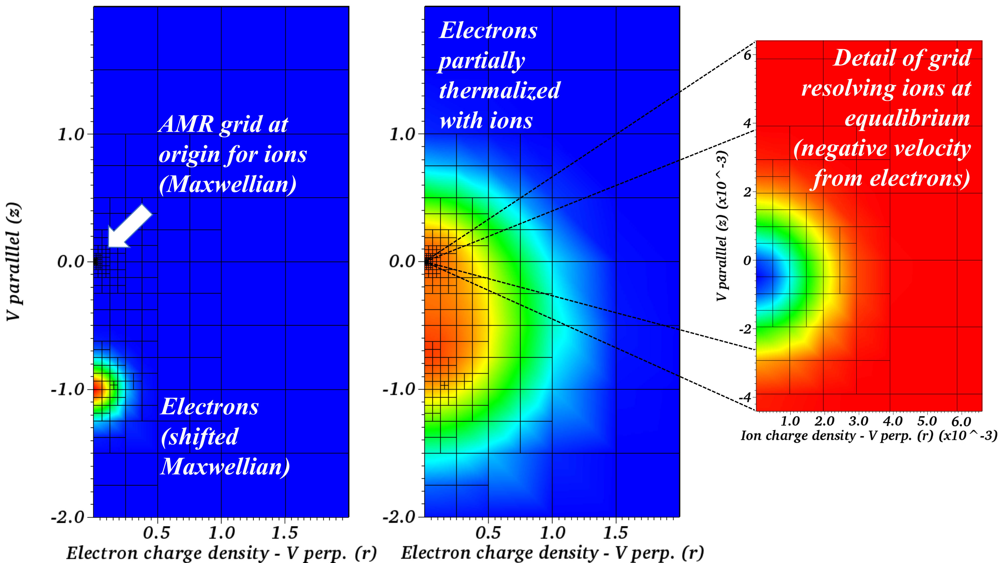
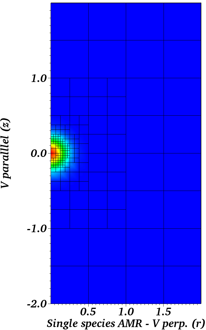
Figure 1: Charge density with initial Maxwellian distribution functions relaxing towards equilibrium, initial electron distribution (left), partially thermalized electrons (center, left), detail of the ion distribution (center, right), electron only adapted mesh (right)

The ions are resolved with AMR at the origin and have a near Maxwellian distribution. Note, Figure 1 uses linear interpolation from the four corners of each quadrilateral, whereas the numerics use bi-quadratic interpolation with nine vertices per quadrilateral, which results in inaccuracy and asymmetries in the plots not present in the numerics.

4.2 Optimization and Performance

Most of the work in the Landau solver is in the inner integral of (4,5) (lines 8-16 in Algorithm 3). This kernel is vectorized with Intel AVX-512 intrinsics. The Landau tensors calculation includes two logarithms, a square root, a power, seven divides, about 85 multiplies and 165 total flops. The power is converted to a inverse square root, an intermediate divide is reused, resulting in five divides, two logarithms, a square root, and an inverse square root. The KNL sockets used for this study is equipped with 34 tiles, each with a 1 megabyte shared L2 cache and two cores, each core has two 8 lane vector units that can issue one fused multiply add (FMA) per cycle per lane. Each core has four hardware threads, for a total of 272 threads per socket. The KNL clock rate is 1.4 GHz, but is clocked down to 1.2 GHz in AVX-512 code segments. This results in a theoretical flop peak rate of $2.6\times 10^{12}$ flops/second. The peak flop rate that can be achieved with this solver is reduced because the kernel is not entirely composed of FMAs and the four logarithms and square roots require considerably more than one cycle each.

The performance data in this section uses a simplified version the test problem, a grid adapted for electrons only with 176 cells and 1,584 quadrature points, a mass ratio of $\frac{m_{i}}{m_{e}}=1$ and $T_{e}=T_{i}=0.2$, and no Maxwellian shifts ($s_{i}=s_{e}=0$), as shown in Figure 1 (right).

Performance overview

The major code segments have been instrumented with PETSc timers. Table 1 show the maximum time from any process for major components of the Landau operator, the total Landau operator, and the linear solver.

Component (times called)	Time (maximum)	% of total
Landau initial vector data setup, Algorithm 2	0.019	2
Landau kernel with AVX512 intrinsics	0.533	66
Landau FE transforms & assemble	0.030	4
Landau FE global matrix assembly	0.072	9
Landau operator total (2)	0.682	85
Linear solver (1)	0.12	15
Total time step time (1)	0.803	100

Table 1: Major component times (maximum of any process) from one time step with two species, double precision and 272 processes

This data is from the double precision solve with 272 processes and two species in Table 4. This data shows that the Landau kernel, though vectorized, is still responsible for most of the run time.

Performance and complexity analysis

There are two types of work in the kernel: 1) computing the two Landau tensors and 2) the accumulation of $\bm{K}$ vector and $\mathbf{D}$ tensor. The accumulation requires $20S^{2}$ flops (lines 12-13 in Algorithm 3). Instrumenting this inner loop would be invasive, but we can infer the percentage of time and work in these two parts with a complexity model and global measurements. Assume both the time and work cost of the entire solver are of the form $C=aS^{0}+bS^{1}+cS^{2}$. The solve time and flop counts with $S=1,2,3$, shown in Table 2, generate right hand sides for system of three equations and three unknows $a,b$, and $c$, which are the time spent, or work, in each of the three types of components.

# Species	1 proc.	272 proc.	Gflops 1 proc.	Gflops/sec. (% of peak)
1	0.21	0.47	1.01	572 (22)
2	0.28	0.79	1.34	455 (18)
3	0.38	1.38	1.88	370 (14)

Table 2: Time (seconds) with 1 and 272 processes on one KNL socket; flop counts from Intel SDE, and flop rates

The Landau tensor cost is formally independent of the number of species, and the work in the accumulation has $\mathcal{O}(S^{2})$ work complexity. Most of the rest of the costs, given a mesh, order of elements, etc., has $\mathcal{O}(S^{1})$ complexity. Table 3 shows the percentage of time and work in each component, infered from the data in Table 2.

Work type	Flops %	Time %
$S^{0}$ (Landau tensors)	88	81
$S^{1}$ (non-kernel work)	1.5	12
$S^{2}$ (accumulation)	10.5	7

Table 3: Percentage of flops and time in species independent work, work linear in $S$, and work quadratic in $S$, with two species, double precision, and one process

This analysis shows that about $98\%$ of the work, and about $88\%$ of the time, is in the kernel with one process. The measurements of the kernel time in Table 1 is $66\%$ with 272 processes. This discrepancy is probably due to performance noise and memory contention in the 272 process timings. The non-kernel time percentage (12) increases by a factor of about eight from the flop percentage (1.5), which reflects the eight vector lanes of the KNL vector unit.

Memory performance

Our experiments are trivially parallel, but memory contention results in performance degradation as more processes are used on a socket. KNL’s architecture allows for twice as many vector lanes with single (32 bit) versus double (64 bit) precision and can thus run, in theory twice as fast in single precision. This section investigates memory issues with a weak speedup study in single and double precision. Table 4 shows timing data with increasing number of processes on a single KNL socket, with single and double precision.

Processes	272	136	68	34	1
Single	0.51	0.29	0.18	0.17	0.17
Double	0.80	0.46	0.30	0.28	0.28

Table 4: Weak speedup time (seconds) with single and double precision

This data shows that we are achieving about $80\%$ of the perfect factor of two speedup with single precision.

A KNL socket has 136 vector units. One might expect that using more processes than 136 would not be useful, however, the kernel has serial dependancies that result in bubbles in the pipeline, especially in the ninth and tenth order polynomial evaluations in the elliptic integrals. These holes can be filled by interleaving a second process in the second hardware thread. We do see about a 15% increase in total performance from the added parallelism of using 272 processes. This data shows that the flop rate per process decreases by a factor of about 3 in going from one process per tile to two processes per vector unit, or eight processes per tile. There is no difference between the one process and 34 process runs, suggesting that the 34 processes are indeed placed with one per tile. There is little degradation going from one to two processes per tile, suggesting that the problem still fits in the L2 cache. The degradation from one to two processes per core is from L1 cache misses because four processes should be able to fit into the 1 megabyte L2 cache. Analysis of memory complexity and the time data going from one to two processes per vector unit suggest that the full 272 process runs fit in the L2 cache, or nearly so.

4.3 Verification

Consider a convergence study with Cartesian grids of the third moment, thermal flux, to verify the expected order of convergence. An analytical flux for this problem does not exist. Richardson extrapolation is used to construct an approximate exact flux. The mass ratio is $4$, $T_{e}=0.2$ and $T_{i}=0.02$. The flux history, with a series of refined grids starting with a $8\times 16$ grid, is shown in Figure 2 (top, left). Figure 2 also shows the differences between fluxes on successive grids, and the error convergence.

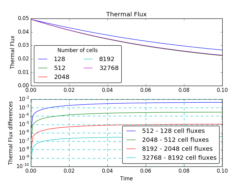
(a) Thermal flux (top), and flux differences

(b) Error vs. cell count

Figure 2: (a) Therm flux over time (top, left), flux differences in grid sequence (bottom, left), quartic convergence rate (right)

We can see from this data that we achieve fourth order convergence.

5 Closure

We have implemented a high order accurate finite element implementation of the Landau collision integral with adaptive mesh refinement in the PETSc library using AVX-512 intrinsics for the Second Generation Intel Xeon Phi, Knights Landing, processor. We have developed a memory centric algorithm for emerging architectures that is amenable to vector processing. We have achieved up to 22% of the theoretical peak flop rate of KNL and analyzed the performance characteristics of the algorithm with respect to process memory contention, single and double precision, and the results of vectorization. We have verified fourth order accuracy with a bi-quadratic, Q2, finite element discretization. Future work includes, building models for runaway electrons in tokamak plasmas with this kernel [15, 8, 17, 7], and building up complete kinetic models (6D AMR) that also preserve the geometric structure of the governing equations of fusion plasmas [16].

6 Acknowledgments

We are grateful for discussions and insights from Intel engineer Vamsi Sripathi. This work has benefited from many discussions with Sam Williams. This work was partially funded from the Intel Parallel Computing Center program. This research used resources of the National Energy Research Scientific Computing Center, a DOE Office of Science User Facility supported by the Office of Science of the U.S. Department of Energy under Contract No. DE-AC02-05CH11231.

References

- [1] Exascale requirements review for fusion energy sciences, 2016, https://www.orau.gov/fesexascale2015 (accessed 2016-01-31).
- [2] S. Balay, S. Abhyankar, M. Adams, J. Brown, P. Brune, K. Buschelman, L. Dalcin, V. Eijkhout, W. Gropp, D. Kaushik, M. Knepley, L. Curfman McInnes, K. Rupp, B. Smith, S. Zampini, H. Zhang, and H. Zhang, PETSc users manual, Tech. Report ANL-95/11 - Revision 3.7, Argonne National Laboratory, 2016, http://www.mcs.anl.gov/petsc.
- [3] S. Balay, S. Abhyankar, M. Adams, J. Brown, P. Brune, K. Buschelman, L. Dalcin, V. Eijkhout, W. Gropp, D. Kaushik, M. Knepley, L. Curfman McInnes, K. Rupp, B. Smith, S. Zampini, H. Zhang, and H. Zhang, PETSc Web page. http://www.mcs.anl.gov/petsc, 2016, http://www.mcs.anl.gov/petsc.
- [4] N. Barral, M. G. Knepley, M. Lange, M. D. Piggott, and G. J. Gorman, Anisotropic mesh adaptation in Firedrake with PETSc DMPlex, in 25th International Meshing Roundtable, S. Owen and H. Si, eds., Washington, DC, September 2016.
- [5] E. A. Belli and J. Candy, Gyrokinetics with Advanced Collision Operators, in APS Meeting Abstracts, Oct. 2014.
- [6] P. Bonoli and L. Curfman McInnes, Report of the workshop on integrated simulations for magnetic fusion energy sciences, 2015, http://science.energy.gov/~/media/fes/pdf/workshop-reports/2016/ISFusionWorkshopReport_11-12-2015.pdf (accessed 2015-06-30).
- [7] A. H. Boozer, Runaway electrons and magnetic island confinement, Physics of Plasmas, 23 (2016), p. 082514, doi:10.1063/1.4960969, http://dx.doi.org/10.1063/1.4960969.
- [8] J. Decker, E. Hirvijoki, O. Embreus, Y. Peysson, A. Stahl, I. Pusztai, and T. Fulop, Numerical characterization of bump formation in the runaway electron tail, Plasma Physics and Controlled Fusion, 58 (2016), p. 025016, http://stacks.iop.org/0741-3335/58/i=2/a=025016.
- [9] C. Greenfield and R. Nazikian, Report on scientific challenges and research opportunities in transient research, 2015, http://science.energy.gov/~/media/fes/pdf/program-news/Transients_Report.pdf (accessed 2015-06-30).
- [10] R. Hager, E. Yoon, S. Ku, E. D’Azevedo, P. Worley, and C. Chang, A fully non-linear multi-species fokker–planck–landau collision operator for simulation of fusion plasma, Journal of Computational Physics, 315 (2016), pp. 644–660, doi:10.1016/j.jcp.2016.03.064, http://dx.doi.org/10.1016/j.jcp.2016.03.064.
- [11] E. Hirvijoki and M. Adams, Conservative Discretization of the Landau Collision Integral, ArXiv e-prints, (2016), arXiv:1611.07881.
- [12] T. Isaac, C. Burstedde, L. C. Wilcox, and O. Ghattas, Recursive algorithms for distributed forests of octrees, SIAM J. Scientific Computing, 37 (2015), doi:10.1137/140970963.
- [13] L. Landau, Kinetic equation for the coulomb effect, Phys. Z. Sowjetunion, 10 (1936), p. 154.
- [14] X. S. Li, An overview of SuperLU: Algorithms, implementation, and user interface, ACM Trans. Math. Softw., 31 (2005), pp. 302–325, doi:10.1145/1089014.1089017, http://doi.acm.org/10.1145/1089014.1089017.
- [15] C. Liu, D. P. Brennan, A. Bhattacharjee, and A. H. Boozer, Adjoint fokker-planck equation and runaway electron dynamics, Physics of Plasmas (1994-present), 23 (2016), p. 010702.
- [16] P. J. Morrison, Structure and structure-preserving algorithms for plasma physics, ArXiv e-prints, (2016), arXiv:1612.06734.
- [17] E. Nilsson, J. Decker, Y. Peysson, R. S. Granetz, F. Saint-Laurent, and M. Vlainic, Kinetic modeling of runaway electron avalanches in tokamak plasmas, Plasma Physics and Controlled Fusion, 57 (2015), 095006, p. 095006, doi:10.1088/0741-3335/57/9/095006, arXiv:1503.06082.
- [18] J. Rudi, A. C. I. Malossi, T. Isaac, G. Stadler, M. Gurnis, P. W. J. Staar, Y. Ineichen, C. Bekas, A. Curioni, and O. Ghattas, An extreme-scale implicit solver for complex pdes: Highly heterogeneous flow in earth’s mantle, in Proceedings of the International Conference for High Performance Computing, Networking, Storage and Analysis, SC ’15, New York, NY, USA, 2015, ACM, pp. 5:1–5:12, doi:10.1145/2807591.2807675. A winner of the Gordon Bell Prize for special achievement.
- [19] G. Stadler, M. Gurnis, C. Burstedde, L. C. Wilcox, L. Alisic, and O. Ghattas, The dynamics of plate tectonics and mantle flow: From local to global scales, Science, 329 (2010), pp. 1033–1038, doi:10.1126/science.1191223.