Low-rank Label Propagation for
Semi-supervised Learning with 100 Millions Samples

Abstract

The success of semi-supervised learning crucially relies on the scalability to a huge amount of unlabelled data that are needed to capture the underlying manifold structure for better classification. Since computing the pairwise similarity between the training data is prohibitively expensive in most kinds of input data, currently, there is no general ready-to-use semi-supervised learning method/tool available for learning with tens of millions or more data points. In this paper, we adopted the idea of two low-rank label propagation algorithms, GLNP (Global Linear Neighborhood Propagation) and Kernel Nyström Approximation, and implemented the parallelized version of the two algorithms accelerated with Nesterov’s accelerated projected gradient descent for Big-data Label Propagation (BigLP). The parallel algorithms are tested on five real datasets ranging from 7000 to 10,000,000 in size and a simulation dataset of 100,000,000 samples. In the experiments, the implementation can scale up to datasets with 100,000,000 samples and hundreds of features and the algorithms also significantly improved the prediction accuracy when only a very small percentage of the data is labeled. The results demonstrate that the BigLP implementation is highly scalable to big data and effective in utilizing the unlabeled data for semi-supervised learning.

1 Introduction

Semi-supervise learning is particularly helpful when only a few labeled data points and a large amount of unlabelled data are available for training a classifier. The unlabelled data are utilized to capture the underlying manifold structure and clusters by smoothness assumption such that the information from the labelled data points can be propagated through the clusters along the manifold structure. Graph-based semi-supervised learning algorithms perform label propagation in a positively-weighted similarity graph between the data points [18, 2]. With the initialization of the vertices of the labeled data, the labels are iteratively propagated between the neighboring vertices and the propagation process will finally converge to the unique global optimum minimizing a quadratic criterion [17]. To construct the similarity graph for label propagation, the commonly used and well accepted measure is Gaussian kernel similarity. The Gaussian kernel applies a non-linear mapping of the data points from the original feature space to a new infinite-dimensional space and computes a positive kernel value for each pair of data points as the similarity in the graph. Since computing the pairwise similarity between the training data is prohibitively expensive under the presence of a huge amount of unlabelled data, no general label propagation method/tool is available for learning with tens of millions or more data points.

In this paper, we propose to improve the scalability of label propagation algorithms with a method based on both low-rank approximation of the kernel matrix, and parallelization of the approximation algorithms and label propagation, named BigLP (Big-data label propagation). We first adopted two low-rank label propagation algorithms, GLNP (Global Linear Neighborhood Propagation) [13] and Kernel Nyström Approximation [14], and implemented the parallelized algorithms. Specifically, GLNP was accelerated with Nesterov’s accelerated projected gradient descent and implemented with OpenMP for shared memory, and Kernel Nyström Approximation was implemented with Message Passing Interface (MPI) for distributed memory. The low-rank approximation and the parallelization of the algorithms allowed the scalability of label propagation up to 100 million samples in our experiments. The low-rank approximation of the kernel graph preserved the useful information in the original uncomputable similarity graph such that the classification results are similar or often better than the original label propagation or supervised learning algorithms that only use labeled data points. Overall, our results suggest that BigLP is effective and ready-to use implementation that will be greatly helpful for big data analysis with semi-supervise learning.

2 Graph-based Semi-Supervised Learning

In this section, we first review the graph-based semi-supervised learning for label propagation and then introduce the two methods for low-rank approximation of the similarity graph matrix for scalable label propagation.

2.1 Label Propagation

In a given dataset $\mathcal{X}=\{x_{1},\ldots,x_{l},\ldots,x_{n}\}$ and a given label set $\mathcal{L}=\{+1,-1\}$, $\{x_{1},\ldots,x_{l}\}$ are data points in $\mathbb{R}^{m}$ labeled by $\{y_{1},\ldots,y_{l}|y_{i}\in\mathcal{L},i=1,\dots,l\}$ and $\{x_{l+1},\ldots,x_{n}\}$ are unlabeled data points in $\mathbb{R}^{m}$. In graph-based semi-supervised learning, a similarity graph $G=(V,E)$ is first constructed from the dataset $\mathcal{X}$, where the vertex set $V=\mathcal{X}$ and the edges $E$ are weighted by adjacency matrix $W$ computed by Gaussian kernel as $W_{ij}=\exp(-\frac{\left\|x_{i}-x_{j}\right\|^{2}}{2\sigma^{2}})$, where $\sigma$ is the width parameter of the Gaussian function. Let $S=D^{-1/2}WD^{-1/2}$, where $D$ is a diagonal matrix with $D_{ii}$ equal to the sum of the $i$th row of W. By relaxing the class label variables as real numbers, label propagation algorithm iteratively updates the predicted label $f$ by

(2.1) $$f^{t+1}=\alpha Sf^{t}+(1-\alpha)f_{0},$$

where $t$ is the step, and $\alpha\in(0,1)$. $f_{0}$ is a vector encoding the labeling of data points from set $\mathcal{L}$ and 0 is assigned to the unlabeled data. After running label propagation, the labels of the data points $\{x_{l+1},\ldots,x_{n}\}$ are assigned based on $f^{*}$.

2.2 Low-rank Label Propagation

In large-scale semi-supervised learning, the number of samples can be in the order of tens of millions or more, leading to the difficulty in storing and operating the adjacency matrix $W$. A general solution is to generate a low-rank approximation of $W$. Specifically, the $n{\times}n$ symmetric positive semi-definite kernel matrix $W$ can be approximated by $W\approx FF^{T}$, where $F\in\mathbb{R}^{n{\times}k}$ and $k{\ll}n$. Let $\bar{F}$ denotes the normalized $F$ with

(2.2) $$\bar{F}_{ij}=\frac{F_{ij}}{\sqrt{F_{i,:}\sum{F}}}$$

where $F_{i,:}$ represents row $i$ of $F$, $\sum{F}$ is a vector composed by the sum of each column of $F$, and $S\approx\bar{F}\bar{F}^{T}$. With the approximation, Eqn. (2.1) can be rewritten as

(2.3) $$f^{t+1}=\alpha{\bar{F}}{\bar{F}^{T}}f^{t}+(1-\alpha)f_{0}.$$

In this new formula, the computational and memory requirements associated with handing the matrix $\bar{F}$ is $O(kn)$, which is much lower than $O(n^{2})$. Nyström Method [14] and Global Linear Neighborhood Propagation (GLNP) [13] were previously proposed to learn the low rank approximation for label propagation.

As shown in [17], the closed-form solution of Eqn. (2.3) can be directly derived

(2.4) $$f^{*}=\lim_{t\to\infty}f^{t}=(1-\alpha)(I_{n}-\alpha\bar{F}\bar{F}^{T})^{-1}f_{0},$$

where $I_{n}$ denotes the $n\times n$ identity matrix. Taking advantage of the low-rank structure of $I_{n}-\alpha\bar{F}\bar{F}^{T}$, applying Matrix-Inversion Lemma [15] generates a simplified solution as

(2.5) $$(I_{n}-\alpha\bar{F}\bar{F}^{T})^{-1}=I_{n}-\bar{F}(\bar{F}^{T}\bar{F}-(1/\alpha)I_{k})^{-1}\bar{F}^{T}.$$

In this solution, the $k\times k$ matrix $\bar{F}^{T}\bar{F}-(1/\alpha)I_{k}$ needs to be inverted instead of the $n\times n$ matrix $I_{n}-\alpha\bar{F}\bar{F}^{T}$. Overall, the time complexity of computing the closed-form solution $f^{*}$ is $O(k^{3}+nk)$, which is a better choice for small $k$, compared with the time complexity of iterative Eqn. (2.3) which is $O(knT)$ where $T$ is the total number of iterations for convergence.

2.3 Nyström Method

Let $W_{ij}=w(x_{i},x_{j})$ for a kernel function $w(a,b)=\langle\Phi{(a)},\Phi{(b)}\rangle$, where $a,b\in\mathcal{X}$ and $\Phi$ is a mapping function. The Nyström method generates low-rank approximations of $W$ using a subset of the samples in $\mathcal{X}$ [14]. Suppose $k\ll n$ data points { $\bar{x}_{1},\bar{x}_{2},...,\bar{x}_{k}$ } are sampled from $\mathcal{X}$ without replacement and let $G$ be the $k{\times}k$ kernel matrix of the random samples, where $G_{i,j}=w(\bar{x}_{i},\bar{x}_{j})$. Let $C$ be the $n$ by $k$ kernel matrix between $\mathcal{X}$ and the random samples, where $C_{i,g}=w(x_{i},\bar{x}_{g})$. The kernel matrices $W$ and $C$ can be written in blocks as

$$W=\begin{bmatrix}G&W_{21}^{T}\\ W_{21}&W_{22}\end{bmatrix}\text{and }C=\begin{bmatrix}G\\ W_{21}\end{bmatrix}.$$

$G$ and $C$ can be applied to construct a rank-$k$ approximation to $W$:

(2.6) $$W\approx CG_{k}^{+}C^{T}=FF^{T},$$

where $G_{k}^{+}$ is the pseudo-inverse of $G$ and the low rank matrix ${F}=C\sqrt{G_{k}^{+}}$, where $\sqrt{G_{k}^{+}}$ denotes element-wise square root of $G_{k}^{+}$, can be computed to approximate $W$ for low-rank label propagation in Eqn. (2.1).

Instead of selecting $k$ random data points, $k$-means clustering could be applied to construct Nyström low-rank approximation. The $k$ centroids obtained from the $k$-means were used as the landmark points to improve the approximation over random sampling [16].

2.4 Global Linear Neighborhood Propagation

Another strategy to learn the low rank representation is through global linear neighborhood [13]. Global linear neighborhood propagation (GLNP) was proposed to preserve the global cluster structures by exploring both the direct neighbors and the indirect neighbors in [13]. It is shown that global linear neighborhoods can be approximated by a low-rank factorization of an unknown similarity graph. Let $X$ be the $n\times m$ data matrix from $\mathcal{X}$ where $X_{ij}$ is the value of the data point $x_{i}$ at the $j$th dimension. Instead of selecting $k$ neighbors to construct the similarity graph, GLNP learns a non-negative symmetric similarity graph by solving the following optimization problem:

(2.7) $$\min\mathcal{Q}(F)=\left\|X-FF^{T}X\right\|^{2}$$

subject to $F_{ij}\geq 0$ where $F$ is a $n\times k$ matrix. To solve Eqn. (2.7), a multiplicative updating algorithm for nonnegative matrix factorization was proposed in [13]. Assume that $X$ contains only nonnegative values, a nonnegative $F$ can be learned by the following multiplicative update rule:

(2.8) $$F_{ij}\leftarrow F_{ij}\times\sqrt{\frac{(2XX^{T}F)_{ij}}{(FF^{T}XX^{T}F+XX^{T}FF^{T}F)_{ij}}},$$

where $\times$ represents element-wise multiplication. After $F$ is learned, it can be used for label propagation.

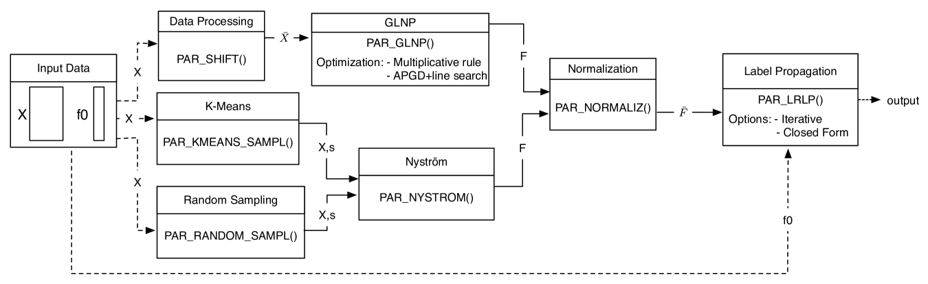
Figure 1: Diagram of the implementation architecture. Each step is described and annotated with the function name in the parallel implementation. The input data are data matrix $X$ and initial labeling $y_{0}$. $X$ is first pre-processed (for GLNP). The data matrix is then used as input data for GLNP or Nyström algorithms using $k$-means or random sampling. Finally, the low-rank matrix is normalized and label propagation is run on the normalized low rank matrix and the input labeling $f_{0}$.

2.5 Accelerated Projected Gradient Descent

The objective function $\mathcal{Q}(F)$ in Eqn. (2.7) is a fourth order non-convex function of $F$ similar to the symmetric NMF problem in [7]. For large-scale data, a first-order optimization method is preferred to find a stationary point [3]. Applying the gradient descent method $a^{r+1}=a^{r}-\frac{1}{L}\nabla f(a^{r})$ to a convex Lipschitz continuous function $f(a)$ with $||\nabla f(a)-\nabla f(b)||\leq L||a-b||$, the rate of convergence after $r$ steps is $O(1/r)$ satisfying $f(a^{r}-a^{*})\leq\frac{2L||a^{0}-a^{*}||^{2}}{r+3}$. In [10], an optimal first order Nesterov’s method was proposed to achieve $O(1/r^{2})$ convergence rate with $f(a^{r}-a^{*})\leq\frac{2L||a^{0}-a^{*}||^{2}}{r^{2}}$. Since Nesterov’s method is often used to accelerate the projected gradient descent to solve constraint optimization problems [1, 11]. Here we adopt Nesterov’s accelerated projected gradient descent method to minimize the objective function $\mathcal{Q}(F)$ in Eqn. (2.7) in Algorithm 1.

1:initialize $Y^{1}=F^{0}$, $\gamma_{1}=1$

2:for $t=1\to maxIter\do$ do

3:     $F^{t}=P[Y^{t}-\alpha_{t}\nabla\mathcal{Q}(Y^{t})/||\nabla\mathcal{Q}(Y^{t})||]$

4:     $\gamma_{t+1}=\frac{1+\sqrt{1+4\gamma_{t}^{2}}}{2}$

5:     $Y^{t+1}=F^{t}+(\frac{\gamma_{t}-1}{\gamma_{t+1}})(F^{t}-F^{t-1})$

6:     if $||\nabla^{P}\mathcal{Q}(F^{t})||\leq\epsilon||\nabla\mathcal{Q}(F^{0})||$ then

7:         $break$

8:     end if

9:end for

10:return $F$

Algorithm 1 Accelerated Projected Gradient Descent

The operation $P[C]$ denotes projecting $C$ into the nonnegative orthant such that:

$$P[C]=\begin{cases}0,&\text{if}\ \ C<0\\ C,&\text{otherwise}\end{cases}$$

$\nabla^{P}\mathcal{Q}(F)$ is the projected gradient of variable $F$ defined as:

$$(\nabla^{P}\mathcal{Q}(F))_{ij}=\begin{cases}(\nabla\mathcal{Q}(F))_{ij},&\text{if}\ \ F_{ij}\geq 0\\ \text{min}(0\text{, }(\nabla\mathcal{Q}(F))_{ij}),&\text{otherwise}\end{cases}$$

The stopping condition $||\nabla^{P}\mathcal{Q}(F^{t})||\leq\epsilon||\nabla\mathcal{Q}(F^{0})||$ checks if a point $F^{t}$ is close to a stationary point in a bound-constrained optimization problem [8].
The step size $\alpha_{t}$ in the projected gradient descent is chosen by Backtracking line search [3, 8] as: Given $0<\beta<1$ and $0<\sigma<1$, starting with $\alpha_{1}=1$ and shrinking $\alpha$ as $\alpha_{t+1}:=\beta\alpha_{t}$ until the condition $\mathcal{Q}(Y^{t+1})-\mathcal{Q}(Y^{t})\leq\sigma\langle\nabla\mathcal{Q}(Y^{t}),(Y^{t+1}-Y^{t})\rangle$ is satisfied.

3 Parallel Implementation

The architecture of the parallel implementation of the low-rank label propagation algorithms is shown in Figure 1. In this section, we first give a brief overview of the distributed memory and shared memory architecture, and linear algebra libraries used in the implementation, and then describe the parallel implementation of each algorithm.

3.1 Memory Architecture

The parallel computing approach reduces memory requirements on Label Propagation and Nyström low-rank matrix computation with distributed memory architecture. Shared-memory architecture was applied to run GLNP in a single computer with multi-threading.

3.1.1 Distributed Memory:

The distributed memory architecture follows the SPMD (single program, multiple data) paradigm for parallelism. The same program simultaneously runs on multiple CPUs according to the data decomposition. The processes communicate with each other to exchange data, as needed by the programs. The distributed memory architecture allows allocation of dedicated memory to each process possibly running on different machines for better scalability in memory requirement on each machine. The disadvantage is the overhead incurred through the data communication through the network among the machines.

Message Passing Interface (MPI) [6] was used to implement the distributed memory architecture. MPI provides a rich set of interfaces for point-to-point operations and collective communications operations (group operations). In addition, MPI-2 [5] introduces one-sided communications operations for remote memory access. We used MPI to implement the parallel Low-rank Label Propagation and the Nyström approximation. In particular, the implementation of Nyström approximation only requires communication of size $O(n+k^{2})$.

3.1.2 Shared Memory:

The computation of GLNP involves a large number of matrix multiplication operations which, to be performed in parallel with distributed memory, requires too much data communication. Even if distributed memory still considerably reduces the memory requirements, the overall running time could be worse. Therefore, we adopted shared memory architecture in the implementation.

In the shared memory architecture, the program runs in multi-threading with all the threads accessing the same shared memory. There is no incurred overhead in data communication. However, the architecture can only utilize the memory available in one machine. Moreover, the shared memory architecture incurs an overhead of cache coherence, in which threads compete to access the same cache with different data, resulting in high cache misses. We implemented the shared memory architecture using the OpenMP API.

3.2 Linear Algebra Libraries

In all the implementations, OpenBLAS was used to perform basic linear algebra operations. OpenBLAS is an optimized version of the BLAS library, and allows multi-threading implementation. For more advanced linear algebra operations, in the eigen-decomposition for Nyström Approximation, we used the LAPACK library.

3.3 Parallel Nyström Approximation

The parallel Nyström approximation algorithm implements both random and $k$-means sampling of $k$ samples to calculate the low-rank representation. Algorithm S.3 in the Supplementary document describes sampling $k$ random samples without replacement. Algorithm S.4 selects $k$ samples as the centroids learned by $k$-means. For improved efficiency, we typically only run $k$-means with a small number of iterations, which usually generates reasonably good selection.

1:function Par_Nyström($X^{p},X_{k}^{p},m,n,k,maxIter$)

2:     for $i=0\to k-1\do$ do

3:         $MPI\_Broadcast({X_{k}^{p}}_{i},sample,kIdxs_{i})$

4:         $W_{i}=RBF(X_{k}^{p},sample)$

5:         $C_{i}=RBF(X^{p},sample)$

6:     end for

7:     $MPI\_Gather(W,0)$

8:     if $rank=0$ then

9:         $[eigvals,eigvecs]=EIG(W)$

10:     end if

11:     $MPI\_Broadcast(eigvals,0)$

12:     $MPI\_Broadcast(eigvecs,0)$

13:     $G=C*eigvecs$

14:     for $i=0\to k-1\do$ do

15:         $G_{i}=G_{i}/\sqrt{eigvals_{i}}$

16:     end for

17:     return $G$

18:end function

Algorithm 2 Parallel Nyström

Based on the selected $k$ samples, Nyström approximation algorithm is implemented in Algorithm 2. In Algorithm 2, the process assigned with sample $i$ broadcasts sample $i$ to the other processes (line 3). After receiving sample $i$, each process calculates $W$ and $C$ entries between sample $i$ and all the samples at the node, with RBF kernel (lines 4-5). Matrix $W$ is then gathered by process 0 to perform the eigen-decomposition of $W$ (lines 7-10). Note that since $W$ is only $k\times k$, the eigen-decomposition is not expensive for small $k$. Process 0 then broadcasts the eigenvectors and eigenvalues to the other processes at lines 11-12. Each process finally calculates the G based on the received eigenvectors and eigenvalues (lines 13-16).

3.4 Parallel GLNP

We implemented parallel GLNP following the two optimization frameworks presented previously: multiplicative update rule and accelerated projected gradient descent with line search. In the multiplicative update rule, given the input data matrix $X$, the function PAR_SHIFT() in Algorithm S.1 checks the minimum value of $X$ and then adds the minimum value to $X$ to obtain the non-negative matrix $\bar{X}$ since GLNP is based on non-negative multiplicative updating. The implementation of GLNP using multiplicative update rule is described in Algorithm 3.

1:function Par_GLNP_MUL($X,m,n,k,maxIter,tol$)

2:     $F\leftarrow U_{m\times k}[0,1]$

3:     for $t=0\to maxIter\do$ do

4:         $F_{old}=F$

5:         $B=X(X^{T}F)$

6:         $D=F(F^{T}B)$

7:         $G=B(F^{T}F)$

8:         for $i=0\to m-1\do$ do

9:              for $j=0\to k-1\do$ do

10:                  $F_{ij}=F_{ij}sqrt(2B_{ij}/(D_{ij}+G_{ij}))$

11:              end for

12:         end for

13:         if $max(abs(F_{old}-F))<tol$ then

14:              $break$

15:         end if

16:     end for

17:     return $F$

18:end function

Algorithm 3 Parallel GLNP - Multiplicative update rule

In Algorithm 3, $F$ is first randomly initialized with uniform distribution between 0 and 1 in parallel by OpenMP. Then, the multiplicative update rule in Eqn. (2.7) is decomposed into several steps of matrix multiplication for parallelization according to the data dependency (lines 5-7). These operations are performed in multi-threading by the OpenBLAS library. Note that all these multiplications are computed in $O(kn)$. Lines 8-12 update $F$ with the multiplicative rule using the intermediate results in $B$, $C$ and $D$ with openMP. Lines 13-15 check for convergence by the threshold $tol$. Instead of checking the convergence of the objective function, which increase the memory requirements, the algorithm checks the maximum change among the elements in $F$. In our observation, the convergence is always achieved with this criteria.

1:function Par_GLNP_APGD($X$,$m$,$n$,$k$,$maxIter$, ,$maxInnerIter$,$beta$,$tol$,$roll$)

2:     $F\leftarrow U_{m\times k}[0,1]$

3:     $Y=F$

4:     for $t=0\to maxIter\do$ do

5:         $B=X(X^{T}Y)$

6:         $D=Y(Y^{T}B)$

7:         $G=B(Y^{T}Y)$

8:         for $i=0\to m-1\do$ do

9:              for $j=0\to k-1\do$ do

10:                  $Grad_{ij}=2D_{ij}+2G_{ij}-4B_{ij}$

11:              end for

12:         end for

13:         $Grad_{0}=Grad$

14:         $Grad=Grad/sqrt(sum(Grad))$

15:         $obj_{old}=obj$

16:         $obj=||X-Y^{T}YX||^{2}$

17:         $alpha=1$

18:         for $inner=0\to maxInnerIter\do$ do

19:              $Y_{1}=max(Y-alpha.Grad,0)$

20:              $obj_{1}=||X-Y_{1}^{T}Y_{1}X||^{2}$

21:              $sum=\sum(Grad_{0}*(Y_{1}-Y))$

22:              if $obj_{1}-obj<roll.sum$ then

23:                  $break$

24:              end if

25:              $alpha=beta^{inner+1}$

26:         end for

27:         $F_{old}=F$

28:         $F=Y_{1}$

29:         $t_{old}=t$

30:         $t=(1+sqrt(1+4t^{2}))/2$

31:         $Y=F+(F-F_{old})(t_{old}-1)/t$

32:         if $abs((obj_{1}-obj_{old})/obj_{1})<tol$ then

33:              $break$

34:         end if

35:     end for

36:     return $F$

37:end function

Algorithm 4 Parallel GLNP - Projected Gradient Descent with Line Search

Dataset	HEPMASS	SUSY	mnist8m	Protein	Gisette
Sample	$10.5\times 10^{6}$	$5\times 10^{6}$	1,648,890	13,077	7,000
Feature	27	128	784	357	5,000

Table 1: Summary of datasets

The GLNP implementation with projected gradient descent and line search is presented in Algorithm 4. In Algorithm 4, we first calculate the normalized and unnormalized gradient of the objective function (lines 9-15). Line 16 calculates the objective function used by the line search. Lines 18-26 will perform the inner iterations of the projected gradient descent. Finally, the convergence is checked on line 33.

3.5 Parallel Low-rank Label Propagation

After normalizing low rank matrix $F$ by the function PAR_NORMALIZ() in Algorithm S.2 according to Eqn. (2.2), parallel low-rank label propagation is performed on the normalized low-rank data $\bar{F}$ and the initial labeling vector $f^{0}\in\mathbb{R}^{n\times 1}$ with Algorithm S.5. Note that $f^{0}$ is also divided among the processes such that each process contains only a vector ${f^{0}}^{p}\in\mathbb{R}^{\frac{n}{p}\times 1}$. Algorithm S.5 first initializes $f^{p}$ by sampling an uniform distribution between -1 and 1 (line 2). Each process is only responsible for calculating the allocated part of $f$. Lines 5-7 perform label propagation, and lines 8-12 check for convergence. Each process will return the local $f^{p}$.

4 Results

The parallel algorithms are tested on five real datasets and a simulation dataset. The runtime and memory requirement are measured. The prediction accuracy for semi-supervised learning was also reported.

4.1 Datasets

Five datasets with various sample sizes and feature sizes described in Table 1 were downloaded. The two largest datasets, HEPMASS and SUSY, were downloaded from UCI. Each of them contains millions of samples but a small number of features. mnist8m is the handwritten digit data from [9] which contains digits 7 and 9 for classification. The Protein dataset is for protein secondary structure prediction. In the experiments we only selected two out of the three classes for classification. The Gisette dataset is also a handwritten digit dataset used for feature selection challenge in NIPS 2003. Finally, we also created a random simulation dataset, with 100 million samples and 100 features to test the scalability of the implementation.

4.2 Runtime and Memory Requirements

We measured the runtime and memory requirements of our parallel implementation of Nyström (both random sampling and $k$-means sampling) and GLNP in all the datasets, shown in Figures 2 and 3.

Figure 2 shows that GLNP is more scalable up to 4 threads and becomes worst at 8 threads due to the overhead by cache coherence with different threads competing to access the same cache which results in many cache misses. In the SUSY dataset, parallel GLNP with $k=20$ runs 1.89x faster than the serial implementation. In the HEPMASS with $10.5$ millions samples, parallel GLNP is 1.71x faster than the serial implementation. The multithreading by 4 threads clearly reduces the runtime considerably. GLNP was implemented in the shared-memory architecture, which always requires a constant amount of memory independent of the number of threads in Figure 3.

Figure 2 also confirms that Nyström is a very scalable algorithm. Using 8 processes, the parallel implementation of the random sample selection with $k=20$ performs 7.67x faster than the serial implementation on the mnist8m dataset, and 7.48x faster with sample selection by $k$-means. In the HEPMASS dataset, the algorithm was 7.08x faster using random sampling, and 7.42x using $k$-means. In Figure 3, the Nyström implementation reduces the memory requirements on each machine with the distributed memory architecture without introducing much overhead consumption. Note that among the large datasets, mnist dataset has relative more features. The memory consumption for different $k$ is very similar since the original dataset is larger than the low-rank approximation data by a big magnitude.

In Figure 4, the plots show a comparison of the optimization by GLNP with acceleration plus line-search and multiplicative updating on three datasets Gisette, Protein and HEPMASS. In all the three cases, accelerated projected gradient descent achieved a better local optimal. Multiplicative updating has a very fast drop in the objective function in the first iteration and then gets into very slow steps for convergence. In practice, we observed that accelerated projected gradient descent achieves better local optimal and convergence in less iterations in all the experiments.

Finally, we evaluated the performance on the simulation dataset with 100 millions of samples and 100 features. We were able to run this dataset using at least 8 processes by the Nyström implementation. With $k$=20 under random sample selection, the implementation completes in 140 seconds with 8 processes. The implementation under $k$-means sample selection runs in 543 seconds with 16 processes. It is also important to note that the memory requirements by each process is only 6.5 GB when 16 processes are used, which allows the implementation to run even on most personal computers available nowadays.

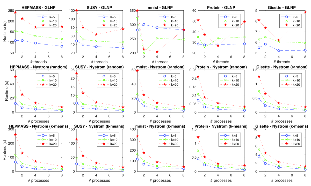
Figure 2: Runtime of GLNP, Nyström (Random) and Nyström ($k$-means).

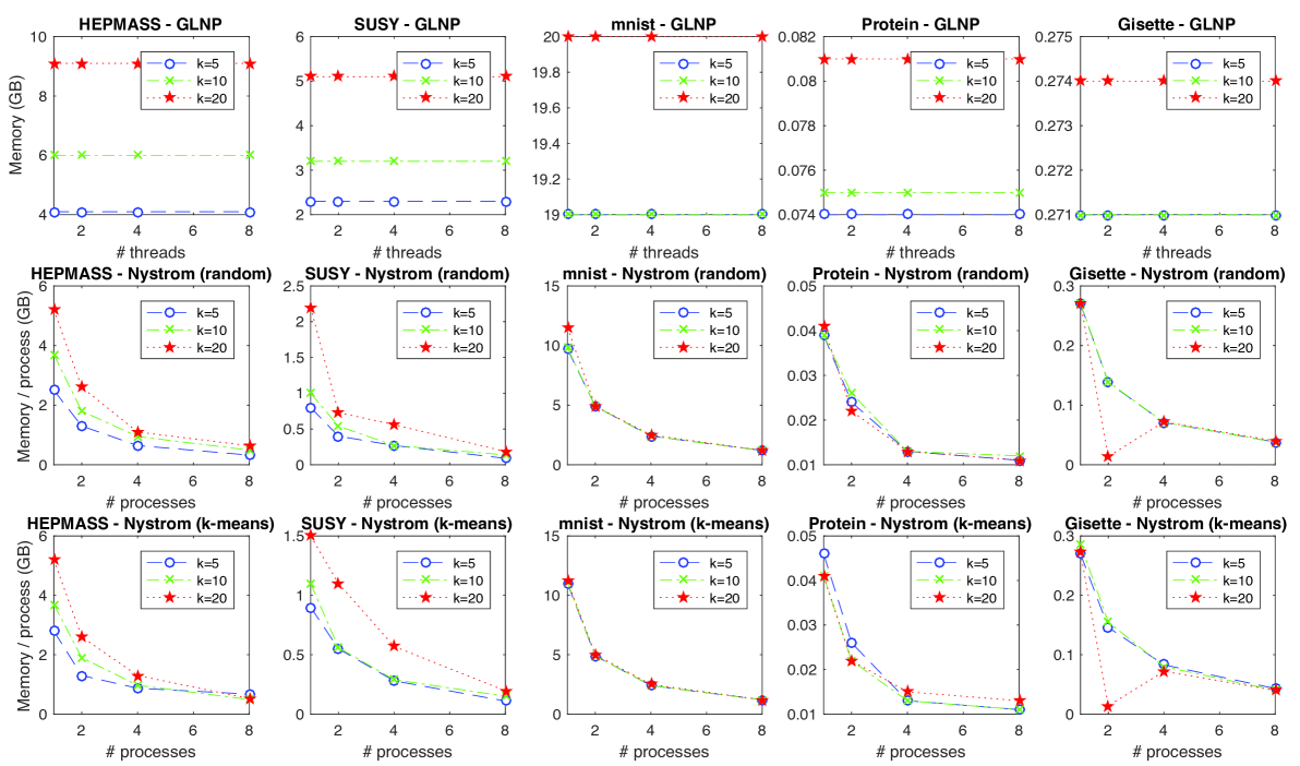
Figure 3: Memory requirements of GLNP, Nyström (Random) and Nyström ($k$-means).

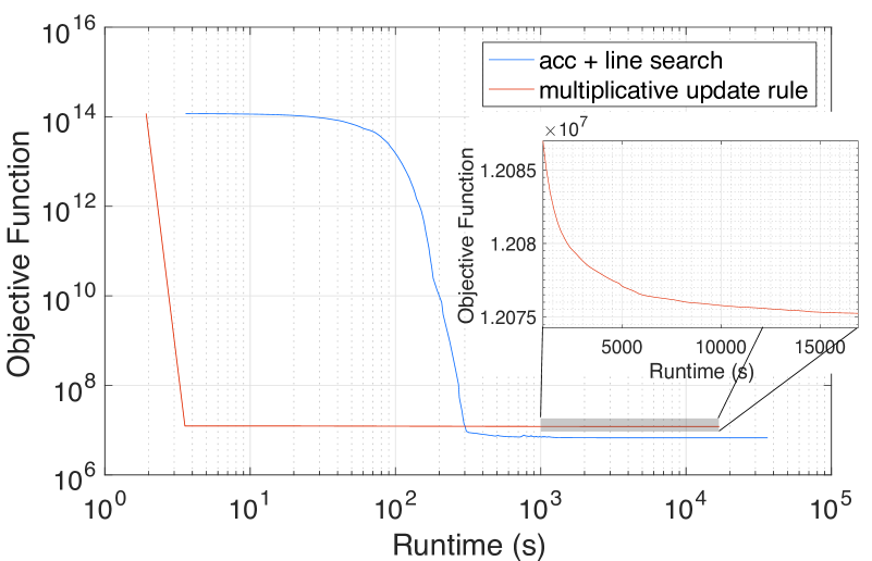
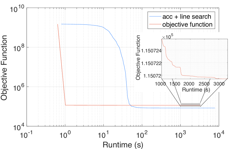
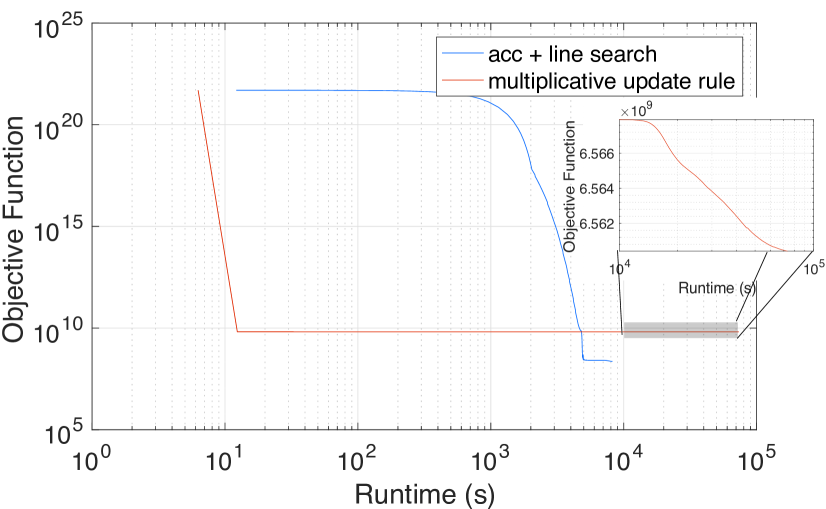
(A) Gisette k=100	(B) Protein k=100	(C) HEPMASS k=10

Figure 4: Comparison of optimization techniques for GLNP. The plots show a comparison of optimization by accelerated projected gradient descent with linear search and multiplicative updating on three datasets.

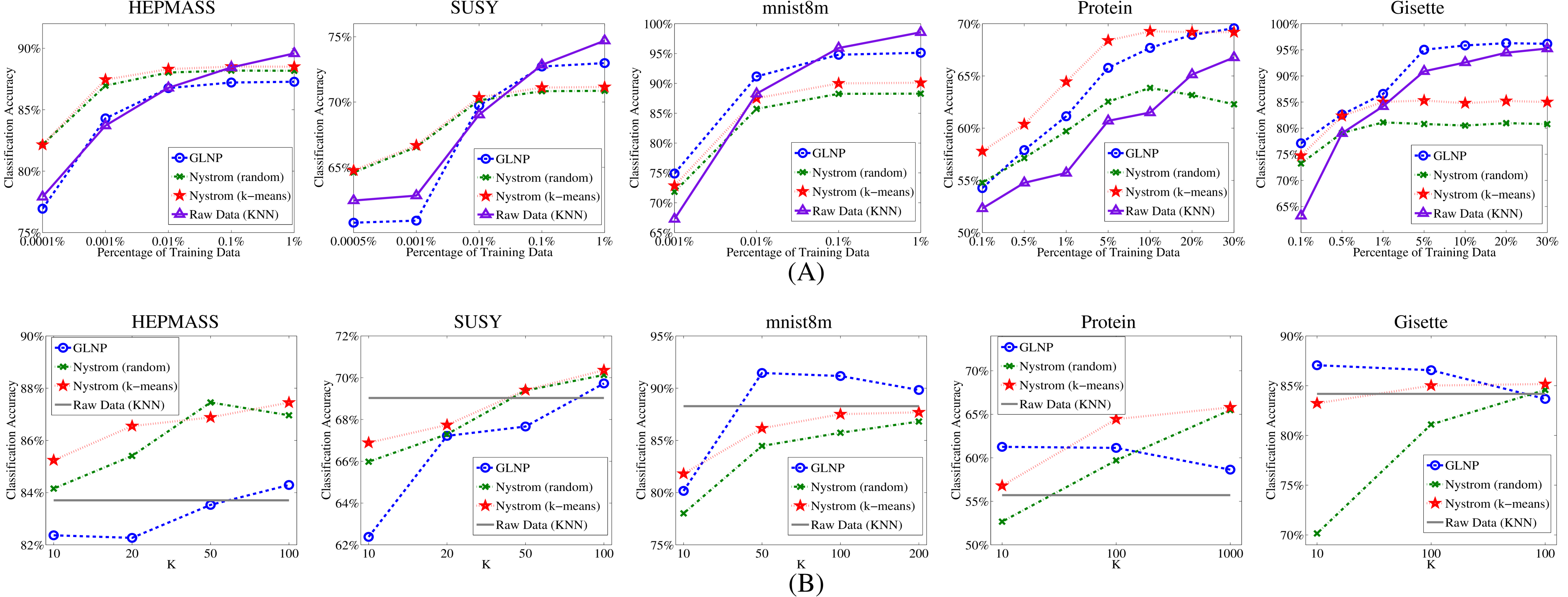
Figure 5: Classification results on five datasets. (A) The x-axis shows percentage of training samples. (B) The x-axis shows $k$ selected to approximate the low-rank matrices.

4.3 Classification on Five Datasets

To test the performance of semi-supervised learning with low-rank matrix approximation, we compared label propagation on the low-rank matrices approximated by GLNP and Nyström approximation (both random sampling and $k$-means sampling) with the $k$-nearest neighbor (KNN) classification algorithm on the original data by considering the five nearest training samples. To evaluate the classification results, we tested different $k$ for low-rank approximation. In the experiments, we held out 20% of samples as the test set, and randomly selected different percentages of samples as the training set in each trail. On each dataset, for each $k$ and each percentage of training samples, we ran 10 trails with different randomly selected training data and report the average classification accuracy on the test set. The same setup was applied to test KNN as a base line. In label propagation, $\alpha$ was set to 0.01.

The classification results are reported in Figure 5. In Figure 5(A), $k$ was fixed to 100 for each experiment and the plots show the results of training with different percentages of training samples. In general, semi-supervised learning by label propagation with low-rank matrix approximation performs better than KNN when only a small size of training data is available. As the size of training data increases, KNN based on all the original features can perform similarly or better on the large datasets. The observation is consistent with the assumption of semi-supervised learning that the underlying manifold structure among labeled and unlabeled data can be explored to improve classification of unlabeled samples when only a small amount of training data is available. As more and more samples become available for training, the structural information becomes less important. Furthermore, low-rank matrix approximation can potentially lose information in the original dataset when $k$ is small. Thus, it is possible that the classification results with low-rank label propagation could be slightly worse than KNN when the size of training data is large. Another observation is that the performance of GLNP is better than Nyström on the small datasets but worse on the large ones. It is possibly because GLNP often requires more iterations to learn the low-rank matrix and convergence is more difficult to achieve on the large datasets. Finally, consistent with previous observations, Nyström with $k$-means sampling consistently is better than random sampling.

In Figure 5(B), the number of training samples were fixed to around 100 for each dataset and results show the effect of choosing different rank $k$. In general, as the size of $k$ increase, the classification performances of low-rank approximation algorithms are closer to the baseline method. In addition, as $k$ increases, the classification performances of Nyström, both $k$-means and random sampling, become better. It is also noticeable that the performance of GLNP is less sensitive to the parameter $k$ since it relies on the global information. Overall, the classification performances of low-rank label propagation are very competitive or better than supervised learning algorithm KNN using the original feature space when $k$ is sufficient. Furthermore, for the largest three datasets, KNN is only scalable to use up to 1$\%$ of samples as training data while the low-rank label propagation are scalable to use all of the training data.

5 Discussion

In this paper, we applied low-rank matrix approximation and Nesterov’s accelerated projected gradient descent with parallel implementation for Big-data Label Propagation (BigLP). BigLP was implemented and tested on the datasets of huge sample sizes for semi-supervised learning. Compared with sparsity induced measures [4] to construct similarity graphs, BigLP is more applicable to the datasets of huge sample size with a relatively small number of features that need to be kernelized for better classification in semi-supervised learning. Sparsity induced measures rely on knowing all the pairwise similarities and would not scale to the datasets with more than hundreds of thousands of samples due to the low scalability in sample size and optimization for sparsity. In addition, compared with the sparsity induced measures and local linear embedding method [12], in which the neighbors are selected “locally”, GLNP preserves the global structures among the data points, and construct more robust and reliable similarity graphs for graph-based semi-supervised learning. In terms of scalability of the two low-rank approximation methods, Nyström approximation is potentially better than GLNP depending on the iterations of $k$-means for sample selection. In practice, the quality of the similarity matrix constructed by Nyström method could also depend on the samples learned by $k$-means which could introduce uncertainty.

6 Funding

The research work is supported by grant from the National Science Foundation (IIS 1149697). RP is also supported by CAPES Foundation, Ministry of Education of Brazil (BEX 13250/13-2).

References

- [1] A. Beck and M. Teboulle, A fast iterative shrinkage-thresholding algorithm for linear inverse problems, SIAM journal on imaging sciences, 2 (2009), pp. 183–202.
- [2] M. Belkin and P. Niyogi, Using manifold stucture for partially labeled classification, in Advances in Neural Information Processing Systems 15, MIT Press, Cambridge, MA, 2003, pp. 929–936.
- [3] D. P. Bertsekas, Nonlinear programming, Athena scientific Belmont, 1999.
- [4] H. Cheng, Z. Liu, and J. Yang, Sparsity induced similarity measure for label propagation, in 2009 IEEE 12th international conference on computer vision, IEEE, 2009, pp. 317–324.
- [5] A. Geist, W. Gropp, S. Huss-Lederman, A. Lumsdaine, E. Lusk, W. Saphir, T. Skjellum, and M. Snir, Mpi-2: Extending the message-passing interface, in European Conference on Parallel Processing, Springer, 1996, pp. 128–135.
- [6] W. Gropp, E. Lusk, N. Doss, and A. Skjellum, A high-performance, portable implementation of the mpi message passing interface standard, Parallel computing, 22 (1996), pp. 789–828.
- [7] D. Kuang, H. Park, and C. H. Q. Ding, Symmetric nonnegative matrix factorization for graph clustering., in SDM, SIAM / Omnipress, 2012, pp. 106–117.
- [8] C.-J. Lin, Projected gradient methods for nonnegative matrix factorization, Neural computation, 19 (2007), pp. 2756–2779.
- [9] G. Loosli, S. Canu, and L. Bottou, Training invariant support vector machines using selective sampling, Large scale kernel machines, (2007), pp. 301–320.
- [10] Y. Nesterov, A method of solving a convex programming problem with convergence rate o (1/k2), in Soviet Mathematics Doklady, vol. 27, 1983, pp. 372–376.
- [11] B. O’Donoghue and E. Candes, Adaptive restart for accelerated gradient schemes, Foundations of computational mathematics, 15 (2015), pp. 715–732.
- [12] S. T. Roweis and L. K. Saul, Nonlinear dimensionality reduction by locally linear embedding, Science, 290 (2000), pp. 2323–2326.
- [13] Z. Tian and R. Kuang, Global linear neighborhoods for efficient label propagation., in SDM, SIAM, 2012, pp. 863–872.
- [14] C. Williams and M. Seeger, Using the Nyström method to speed up kernel machines, in Proceedings of the 14th annual conference on neural information processing systems, no. EPFL-CONF-161322, 2001, pp. 682–688.
- [15] M. A. Woodbury, Inverting modified matrices, Memorandum report, 42 (1950), p. 106.
- [16] K. Zhang, I. W. Tsang, and J. T. Kwok, Improved nyström low-rank approximation and error analysis, in Proceedings of the 25th international conference on Machine learning, ACM, 2008, pp. 1232–1239.
- [17] D. Zhou, O. Bousquet, T. N. Lal, J. Weston, and B. Schölkopf, Learning with local and global consistency, in Advances in Neural Information Processing Systems 16, MIT Press, Cambridge, MA, 2004.
- [18] X. Zhu, Z. Ghahramani, and J. D. Lafferty, Semi-supervised learning using gaussian fields and harmonic functions, in ICML, 2003, pp. 912–919.