Semiparametric Estimation of Symmetric Mixture Models with Monotone and Log-Concave Densities

Abstract

In this article, we revisit the problem of fitting a mixture model under the assumption that the mixture components are symmetric and log-concave. To this end, we first study the nonparametric maximum likelihood estimation (MLE) of a monotone log-concave probability density. To fit the mixture model, we propose a semiparametric EM (SEM) algorithm, which can be adapted to other semiparametric mixture models. In our numerical experiments, we compare our algorithm to that of Balabdaoui and Doss (2014) and other mixture models both on simulated and real-world datasets.

1 Introduction

Mixture models are a staple of statistical analysis. In this paper, we concern ourselves with semi-parametric mixture models under the hypotheses of symmetry and log-concavity.

Consider the following mixture model (in dimension 1) $g(x)=\sum_{j=1}^{k}\pi_{j}f(x-\mu_{j})$, where, as usual, $\pi_{j}\geq 0$ and $\sum_{j}\pi_{j}=1$, $\mu_{j}\in\mathbb{R}$, and $f$ is a density on the real line. Let $\boldsymbol{\pi}=(\pi_{1},\dots,\pi_{k})$ and ${\boldsymbol{\mu}}=(\mu_{1},\dots,\mu_{k})$. Bordes et al. (2006) and Hunter et al. (2007) examine the identifiability of such a model under the assumption that $f$ is symmetric. Their work shows that the model is identifiable when $k=2$ (up to labeling) as long as $\pi_{1}\neq 1/2$. They also consider the case of $k=3$ components and show that identifiability holds except for sets of zero Lebesgue measure. Balabdaoui and Butucea (2014) assume $f$ is a Pólya frequency function of infinite order and show that the model is identifiable (as always, modulo relabeling), regardless of whether $f$ is symmetric or not (in the latter case, $f$ is assumed to have zero mean).

Regardless of identifiability, fitting mixture models to data is common practice in statistics, often as an exploration procedure to uncover interesting features of the underlying distribution (e.g., clusters). In terms of methods for fitting such models, Bordes et al. (2006) use the so-called minimum contrast method to estimate $\boldsymbol{\pi}$ and ${\boldsymbol{\mu}}$, and use a kernel density estimation (KDE) approach which involves a model selection procedure to choose the tuning parameter. Hunter et al. (2007) employ a generalized Hodges-Lehmann estimator to estimate ${\boldsymbol{\mu}}$ and achieve a better rate of convergence. However, their estimator for $f$ is not guaranteed to be a density. Bordes et al. (2007) propose a stochastic EM-like estimation algorithm which does not possess the monotone property of a genuine EM algorithm. Butucea and Vandekerkhove (2014) propose $\sqrt{n}$-consistent M-estimators based on a Fourier approach.

Balabdaoui and Doss (2014) consider the same model with $f$ symmetric and log-concave. Their method for fitting the model consists in adopting the estimators for $\boldsymbol{\pi}$ and ${\boldsymbol{\mu}}$ from (Hunter et al., 2007) and then estimating the density $f$ via maximum likelihood. Chang and Walther (2007) study a more general model, $g(x)=\sum_{j=1}^{k}\pi_{j}f_{j}(x)$, where each $f_{j}$ is assumed to be log-concave. They provide an EM-type algorithm for fitting such a model — however, they do not prove that their algorithm increases the likelihood with every iteration. Hu et al. (2016) study the theoretical properties of the maximum likelihood estimator (MLE) for this same model, although the model is not identifiable as argued in(Walther, 2002).

In the present paper, we consider fitting a mixture model of the form

$$g(x)=\sum_{j=1}^{k}\pi_{j}f_{j}(x-\mu_{j}),\quad\sum_{j=1}^{k}\pi_{j}=1,\quad x\in\mathbb{R},$$ (1)

where each $f_{j}$ is assumed symmetric and log-concave. A density $f$ that is symmetric and log-concave is defined by $h(x)=2f(x)1_{\{x\geq 0\}}$, which is a decreasing log-concave density on $\mathbb{R}_{+}$. We make no claims as regards identifiability of this model. Our goal is to simply fit such a model to data.

In Section 2 we start by examining the maximum likelihood estimation of a symmetric and log-concave density, relying heavily on the work of Rufibach (2006) and Dümbgen and Rufibach (2009). In Section 3 we propose a genuine EM algorithm for fitting the mixture model (1). The algorithm includes a step where the monotone and log-concave MLE for $h_{j}$ is computed. To do so we apply the method of Doss and Wellner (2016b) designed for computing the log-concave MLE with a fixed mode — the mode is of course set to 0 in our case. We note that Balabdaoui and Doss (2014) use the same routine in the numerical implementation of their method. In Section 4 we apply our model to clustering problems and compare our approach with that of (Chang and Walther, 2007) and that of (Balabdaoui and Doss, 2014), as well as a Gaussian mixture model, on both synthetic and real-world datasets.

2 On the maximum likelihood estimation of a monotone and log-concave density

This section is concerned with the maximum likelihood estimation of a monotone log-concave density on $\mathbb{R}_{+}$. Maximum likelihood estimation of a monotone density was first studied by Grenander (1956), while the maximum likelihood estimation of a log-concave density has garnered attention only more recently (Balabdaoui, 2004; Doss and Wellner, 2016a; Balabdaoui et al., 2009; Dümbgen and Rufibach, 2009; Walther, 2002). Our exposition and results below derive from a straightforward adaptation of the thesis work of Rufibach (2006) on the maximum likelihood of a log-concave density, without the additional constraint of monotonicity, published in the form of a research article (Dümbgen and Rufibach, 2009). We do not provide proofs but rather refer the reader to that work for all the technical details.

Let $f$ denote a decreasing and log-concave density on $\mathbb{R}_{+}$. We let $F$ denote the distribution function corresponding to the density $f$ and define

$$\psi(x)=\log f(x).$$ (2)

Requiring that $f$ be monotone and log-concave is equivalent to requiring that $\psi$ is monotone and concave. Based on the sample, which we assume ordered ($x_{1}<x_{2}<\cdots<x_{n}$), the negative log-likelihood at $f$ is given by

$$-\sum_{i=1}^{n}\log f(x_{i})=-n\sum_{i=1}^{n}\psi(x_{i}).$$ (3)

In order to relax the constraint of $f$ being a probability density we follow the technique used by Rufibach (2006) and add a Lagrange term to (3), leading to the functional

$$\Lambda_{n}(\psi)=-\sum_{i=1}^{n}\psi(x_{i})+n\int_{0}^{\infty}\exp\psi(x){\rm d}x.$$ (4)

The MLE of $f$ is $\hat{f}_{n}=\exp\hat{\psi}_{n}$, where $\hat{\psi}_{n}$ is the minimizer of $\Lambda$ over class of functions on $[0,\infty)$ that are non-increasing and concave, that is

$$\hat{\psi}_{n}:=\operatorname*{arg\,min}_{\psi\in\mathcal{MC}}\,\Lambda_{n}(\psi),$$ (5)

where

$$\mathcal{MC}:=\big{\{}\psi:[0,\infty)\to[-\infty,\infty)\ |\ \psi\text{ is non-increasing, concave, proper, and closed}\big{\}}.$$ (6)

The following results from an adaptation of Theorem 2.1 in (Dümbgen and Rufibach, 2009).

Theorem 1 (Existence, uniqueness, and shape).

The MLE $\hat{\psi}_{n}$ exists and is unique. It is linear between sample points and continuous on $[0,x_{n}]$, with $\hat{\psi}_{n}(x)=\hat{\psi}_{n}(x_{1})$ for $x\in[0,x_{1}]$ and $\hat{\psi}_{n}(x)=-\infty$ for $x>x_{n}$.

The following results from an adaptation of Theorem 2.2 in (Dümbgen and Rufibach, 2009).

Theorem 2 (Characterization).

Let $\psi$ be a non-increasing and concave function such that $\{x:\psi(x)>-\infty\}=[0,x_{n}]$. Then, $\psi=\hat{\psi}_{n}$ if and only if

$$\frac{1}{n}\sum_{i=1}^{n}\Delta(x_{i})\leq\int_{0}^{\infty}\Delta(x)\exp\psi(x){\rm d}x$$ (7)

for any $\Delta:[0,\infty)\to\mathbb{R}$ such that $\psi+\lambda\Delta$ is non-increasing and concave for some $\lambda>0$.

For $I\subset\mathbb{R}$ an interval, $\beta\in[1,2]$, and $L>0$, let $\mathcal{H}^{\beta,L}(I)$ be the Hölder class of real-valued functions $g$ on $I$ satisfying $|g(y)-g(x)|<L|y-x|$ if $\beta=1$ and $|g^{\prime}(y)-g^{\prime}(x)|\leq L|y-x|^{\beta-1}$ if $\beta\in(1,2]$, for all $x,y\in I$. The following results from an adaptation of Theorem 4.1 in (Dümbgen and Rufibach, 2009).

Theorem 3 (Uniform consistency).

Assume that $f\in\mathcal{H}^{\beta,L}(I)$ for some exponent $\beta\in[1,2]$, some constant $L>0$, and a compact interval $I\subset\{f>0\}$. Then,

$$\max_{t\in I}\big{|}\hat{f}_{n}(t)-f(t)\big{|}=O_{\mathbb{P}}(\log n/n)^{\beta/(2\beta+1)}.$$ (8)

As pointed out by Dümbgen and Rufibach (2009), this is the minimax rate for densities in that smoothness class, as shown by Khas’minskii (1979), so that, when the density is log-concave and Hölder-$\beta$ (with $\beta\in[1,2]$) in some interval, the log-concave MLE adapts to the proper smoothness in that interval. We believe the same holds under the additional constraint of monotonicity.

3 A semiparametric EM algorithm

We now consider fitting the semiparametric mixture model (1). Model (1) is defined by $\phi:=({\boldsymbol{\mu}};\boldsymbol{\pi};\boldsymbol{f})$, where ${\boldsymbol{\mu}}=(\mu_{1},\dots,\mu_{k})\in\mathbb{R}^{k}$, $\boldsymbol{\pi}=(\pi_{1},\dots,\pi_{k})$ is an element of the simplex in $\mathbb{R}^{k}$, and $\boldsymbol{f}=(f_{1},\dots,f_{k})$ with each $f_{j}$ being a symmetric and log-concave density on $\mathbb{R}$. Under $\phi$, the mixture model is given by

$$g_{\phi}(x)=\sum_{j=1}^{k}\pi_{j}f_{j}(x-\mu_{j}).$$ (9)

Given a sample $\boldsymbol{x}=(x_{1},\dots,x_{n})$, the log-likelihood under parameter $\phi$ is given by

$$L(\phi)=\sum_{i=1}^{n}\log g_{\phi}(x_{i}).$$ (10)

(As is customary, we leave the dependency in $\boldsymbol{x}$ implicit throughout.) As with other mixture models, maximizing $L(\phi)$ directly is difficult and we resort to an EM-type approach. Define the indicator variables $\boldsymbol{z}:=(z_{1},\dots,z_{n})$, where $z_{i}=j$ when $x_{i}$ was sampled from the $j$th component. These allow us to define the complete log-likelihood

$$\bar{L}(\phi;\boldsymbol{z})=\sum_{i=1}^{n}\sum_{j=1}^{k}\mathbb{I}\{z_{i}=j\}\log(f_{j}(x_{i}-\mu_{j})).$$ (11)

An EM algorithm, after some initialization, alternates between computing the expectation of the complete log-likelihood conditional on $\boldsymbol{x}$ under the current value of the parameters, and maximizing the resulting functional with respect to the parameters. Thus, in the expectation step, assuming that the current value of the parameters is $\phi^{*}$, consists in computing

$$\operatorname{\mathbb{E}}_{\phi^{*}}[\bar{L}(\phi;\boldsymbol{z})\mid\boldsymbol{x}],$$ (12)

which turns out to be equal to

$$Q(\phi,\boldsymbol{w}^{*}):=\sum_{i=1}^{n}\sum_{j=1}^{k}w_{ij}^{*}\log(\pi_{j}f_{j}(x_{i}-\mu_{j})),$$ (13)

where

$$w_{ij}^{*}:=\mathbb{P}_{\phi^{*}}(z_{i}=j\,|\,x_{i})=\frac{\pi_{j}^{*}f_{j}^{*}(x_{i}-\mu_{j}^{*})}{\sum_{l=1}^{k}\pi_{l}^{*}f_{l}^{*}(x_{i}-\mu_{l}^{*})}.$$ (14)

The maximization step consists then in maximizing $Q(\phi,\boldsymbol{w}^{*})$ with respect to $\phi$, thus updating the value of the parameters. This leads to the following semiparametric EM (SEM) algorithm:

• E-step:

  • Compute $\boldsymbol{w}$:

    $$w^{t}_{ij}\leftarrow\mathbb{P}_{\phi^{t}}(z_{i}=j\,|\,x_{i})=\frac{\pi^{t}_{j}f_{j}^{t}(x_{i}-\mu_{j}^{t})}{\sum_{l=1}^{k}\pi_{l}^{t}f_{l}^{t}(x_{i}-\mu_{l}^{t})},$$ (15)

    for $i=1,\dots,n$ and $j=1,\dots,k$.

• M-step:

  • Update $\boldsymbol{\pi}$:

    $$\pi_{j}^{t+1}\leftarrow\frac{1}{n}\sum_{i=1}^{n}w_{ij}^{t},\quad j=1,\dots,k.$$ (16)

  • Update ${\boldsymbol{\mu}}$:

    $$\mu_{j}^{t+1}\leftarrow\operatorname*{arg\,max}_{\mu\in\mathbb{R}}\ \sum_{i=1}^{n}w_{ij}^{t}\log f_{j}^{t}(x_{i}-\mu),\quad j=1,\dots,k.$$ (17)

  • Update $\boldsymbol{f}$:

    $$f_{j}^{t+1}(x)\leftarrow\tfrac{1}{2}h_{j}^{t+1}(|x|),\quad h_{j}^{t+1}\leftarrow\operatorname*{arg\,max}_{h\in\mathcal{MC}}\ \sum_{i=1}^{n}w_{ij}^{t}\log h(|x_{i}-\mu_{j}^{t+1}|),\quad j=1,\dots,k.$$ (18)

As a function of $\mu$, the function appearing in (17) is concave due to the fact that $\log f_{j}^{t}$ is concave by construction. In particular, the Golden Section Search can be applied to find $\mu$. In (18), the optimization is over $h$ being a monotone and log-concave density on $[0,\infty)$. The solution corresponds to the weighted MLE based on data $(|x_{1}-\mu_{j}^{t+1}|,\dots,|x_{n}-\mu_{j}^{t+1}|)$ and weights $(w_{1j(t)},\dots,w_{nj(t)})$. in our implementation we apply the function activeSetLogCon.mode in the R package logcondens.mode with mode chosen to be 0.

Our SEM algorithm has the desirable monotonicity property of a true EM algorithm (Dempster et al., 1977; Wu et al., 1983).

Proposition 1 (Monotonicity property).

We $L(\phi^{t})\leq L(\phi^{t+1})$ for all $t\geq 0$.

Proof.

In the algorithm, armed with $\phi^{t}$, we compute the weights $\boldsymbol{w}^{t}$ in the E-step and in the M-step we obtain $\phi^{t+1}$ by maximizing $Q(\phi,\boldsymbol{w}^{t})$ over $\phi$. In particular,

$$Q(\phi^{t+1},\boldsymbol{w}^{t})\geq Q(\phi^{t},\boldsymbol{w}^{t}).$$ (19)

The key in what follows is Jensen’s inequality, which implies that for a set of parameters $\phi=({\boldsymbol{\mu}};\boldsymbol{\pi};\boldsymbol{h})$ and non-negative weights $\boldsymbol{w}^{*}=(w^{*}_{ij})$ such that $\sum_{j}w^{*}_{ij}=1$ for all $i$,

$$L(\phi) =\sum_{i=1}^{n}\log\bigg{(}\sum_{j=1}^{k}\pi_{j}f_{j}(x_{i}-\mu_{j})\bigg{)}$$ (20)

$$=\sum_{i=1}^{n}\log\bigg{(}\sum_{j=1}^{k}w^{*}_{ij}\frac{\pi_{j}f_{j}(x_{i}-\mu_{j})}{w^{*}_{ij}}\bigg{)}$$

$$\geq\sum_{i=1}^{n}\sum_{j=1}^{k}w^{*}_{ij}\log\bigg{(}\frac{\pi_{j}f_{j}(x_{i}-\mu_{j})}{w^{*}_{ij}}\bigg{)}$$

$$=Q(\phi,\boldsymbol{w}^{*})-C(\boldsymbol{w}^{*}),$$ (21)

where $C(\boldsymbol{w}):=\sum_{i=1}^{n}\sum_{j=1}^{k}w_{ij}\log w_{ij}+n\log 2$. The inequality is in fact an equality if the weights $\boldsymbol{w}^{*}$ are the weights associated with $\phi$ as specified in (14). In particular,

$$L(\phi^{t+1})\geq Q(\phi^{t+1},\boldsymbol{w}^{t})-C(\boldsymbol{w}^{t}),$$ (22)

while

$$L(\phi^{t})=Q(\phi^{t},\boldsymbol{w}^{t})-C(\boldsymbol{w}^{t}).$$ (23)

With this, together with (19), we have

$$L(\phi^{t+1}) \geq Q(\phi^{t+1},\boldsymbol{w}^{t})-C(\boldsymbol{w}^{t})$$

$$\geq Q(\phi^{t},\boldsymbol{w}^{t})-C(\boldsymbol{w}^{t})=L(\phi^{t}).\qed$$

Remark 1 (Initialization).

In practice, we initialize $\boldsymbol{w}^{0}$ and $\boldsymbol{h}^{0}$ at the values computed by fitting a Gaussian mixture model (using an EM algorithm) and start with M-step first.

4 Numerical experiments

We present in this section the result of some numerical experiments. We apply our SEM algorithm both on simulated and real data. In Section 4.1 we simulate data from the Gaussian and Laplace mixture models used in (Balabdaoui and Doss, 2014), and in Section 4.2 we apply the SEM algorithm to the well-known Old Faithful Geyser dataset, as done in (Balabdaoui and Doss, 2014).

4.1 Synthetic datasets

As a first example, we use a two-component Gaussian mixture to empirically check the convergence of our SEM algorithm. We sample $n=300$ observations from the Gaussian mixture $0.15\ \mathcal{N}(-1,1)+0.85\ \mathcal{N}(2,1)$ and apply the SEM algorithm to these two datasets respectively. This seems to be the most difficult situation considered in (Bordes et al., 2006). Panels (a), (b), (c), and (d) of Figure 1 show that SEM stabilizes after about 8 iterations for the three Euclidean parameters and the observed data likelihood. As expected, the achieved maximum data likelihood is monotonically increasing as a function of the number of iterations. Panels (e) and (f) show the final MLE for $f_{1},f_{2},g$ and compare that with the truth. The MLE for the symmetric log-concave densities are piecewise exponential, which is consistent with what is described in Theorem 1.

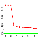
(a) $\pi_{1}^{t}$ as a function of the iteration $t$ (red) and true value (green)

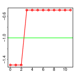
(b) $\mu_{1}^{t}$ as a function of the iteration $t$ (red) and true value (green)

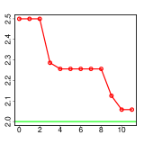
(c) $\mu_{2}^{t}$ as a function of the iteration $t$ (red) and true value (green)

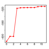
(d) $L(\phi^{t})$ as a function of the iteration $t$

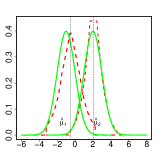
(e) estimated (red, dashed) and true (green, solid) component densities

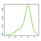
(f) estimated (red, dashed) and true (green, solid) mixture density

Figure 1: SEM for the Gaussian mixture with parameters $k=2,\pi_{1}=0.15,\mu_{1}=-1,\mu_{2}=2$ based on a sample of size $n=300$.

We then compare the performance of our algorithm (SEM) for the problem of clustering with the methods proposed in (Chang and Walther, 2007) and (Balabdaoui and Doss, 2014). Chang and Walther do not assume symmetry while Balabdaoui and Doss assume that the component densities are identical. We denote these two methods by LCM and SLC respectively. We compare SEM, LCM, SLC, and GMM. The latter serves as benchmark when the underlying model is a Gaussian mixture. We compare these methods on two Gaussian mixture models, two Laplace mixture models, and one Gaussian-Laplace mixture model, as described below:

• Model 1: $0.2\,\mathcal{N}(0,1)+0.8\,\mathcal{N}(1,1)$;

• Model 2: $0.2\,\mathcal{N}(0,1)+0.8\,\mathcal{N}(2,2)$;

• Model 3: $0.2\,\mathcal{L}(0,1)+0.8\,\mathcal{L}(1,1)$;

• Model 4: $0.2\,\mathcal{L}(0,1)+0.4\,\mathcal{L}(1.5,1)+0.4\,\mathcal{L}(-1.5,1)$;

• Model 5: $0.2\,\mathcal{N}(0,1)+0.2\,\mathcal{N}(1.5,1)+0.2\,\mathcal{N}(-1.5,1)+0.2\,\mathcal{L}(3,1)+0.2\,\mathcal{L}(-3,1)$.

The sample size is $n=500$ for Models 1-4, while $n=1000$ for Model $5$. Each setting is repeated 1000 times. We examine the quality of the resulting clustering in terms of the achieved data log-likelihood, the misclassification errors when $k=2$ or Rand Indexes when $k\geq 3$, and the average absolute posterior probability error used by (Chang and Walther, 2007) — all averaged over the 1000 repeats. The latter metric investigates how well a mixture clustering algorithm estimates the uncertainty for the membership assignment of each observation on population level. This metric is defined as

$$\text{posterior error}:=\frac{1}{n}\sum_{i=1}^{n}|\hat{w}_{i1}-w_{i1}|,$$ (24)

where $\hat{w}_{i1}$ and $w_{i1}$ are computed by (14) with estimators and true parameters respectively. Notice that this metric only applies to clustering with $k=2$ components. When $k\geq 3$, we define the posterior error using the Frobenius norm,

$$\text{posterior error}:=\min_{\mathbf{P}}\|\hat{\boldsymbol{w}}\mathbf{P}-\boldsymbol{w}\|_{F},$$ (25)

where the minimum is over $k\times k$ permutation matrices $\mathbf{P}$, and matrices $\hat{\boldsymbol{w}}$ and $\boldsymbol{w}$ are computed by (14) based on the MLE and true parameters, respectively. We report the comparison results in Table 1. As can be seen from this table, GMM, LCM, and our SEM algorithm clearly outperform SLC in terms of log-likelihood and posterior error. LCM outperforms other methods in terms of misclassification error or Rand index when $k\leq 3$, but does not perform well when $k=5$. When the mixture densities are normal, SEM performs as well as GMM, arguably the gold standard in such a situation; when the densities are Laplace, SEM slightly improves the clustering initialized by GMM. Moreover, SEM achieves a significantly higher log-likelihood compared with the other methods when the mixture densities are normal. We also notice that SLC sometimes gives better results in terms of misclassification error, even though the posterior-error is worse.

		GMM	LCM	SLC	SEM
Model 1	log-likelihood	-743.2 (0.50)	–739.4 (0.51)	-1104.9 (2.06)	-738.6 (0.50)
	mis-class	122.7 (1.31)	102.6 (1.49)	174.2 (1.22)	123.7 (1.30)
	post-error	0.199 (0.003)	0.206 (0.002)	0.317 (0.001)	0.202 (0.003)
Model 2	log-likelihood	-1049.7 (0.48)	-1046.3 (0.49)	-1383.0 (2.43)	-1044.7 (0.48)
	mis-class	148.1 (1.55)	125.4 (1.91)	118.4 (0.70)	150.0 (1.54)
	post-error	0.211 (0.004)	0.255 (0.003)	0.216 (0.004)	0.283 (0.001)
Model 3	log-likelihood	-876.0 (0.67)	-869.3 (0.69)	-1293.6 (3.94)	-870.6 (0.66)
	mis-class	162.8 (1.12)	111.4 (1.23)	153.2 (1.09)	159.1 (1.18)
	post-error	0.236 (0.002)	0.244 (0.002)	0.324 (0.001)	0.234 (0.002)
Model 4	log-likelihood	-1031.1 (16.8)	-1030.0 (16.6)	-	-1025.7 (16.8)
	Rand index	0.602 (0.097)	0.655 (0.118)	-	0.607 (0.093)
	post-error	10.6 (2.65)	13.3 (1.53)	-	10.6 (2.61)
Model 5	log-likelihood	-2281.8 (19.6)	-2282.9 (20.4)	-	-2276.6 (19.8)
	Rand index	0.617 (0.134)	0.401(0.231)	-	0.619 (0.132)
	post-error	18.2 (3.13)	19.8 (3.25)	-	18.4 (3.21)

Table 1: Comparison of the four different clustering methods in terms of achieved log-likelihood, number of misclassification errors (when $k=2$) or Rand index (when $k>2$), and posterior errors. The reported numbers are averages (and standard deviations) based on 1000 replications. The sample size is $n=500$ for Model 1-4 and $n=1000$ for Model 5. (SLC was only designed for mixtures with $k=2$ components.)

4.2 Real dataset

In this section, we apply our new estimation approach to the Old Faithful Geyser dataset, which consists of times, in minutes, between eruptions of that geyser (found in Yellowstone National Park). Table 2 shows that our estimates (SEM) are close to those obtained by GMM, the method of Hunter et al. (2007) (SP), the method of Bordes et al. (2007) (SP-EM), and the method of Balabdaoui and Doss (2014) (SLC). (SEM converged in about a dozen iterations.)

parameters	GMM	SP	SP-EM	SLC	SEM
$\pi_{1}$	0.361	0.352	0.359	0.33	0.355
$\mu_{1}$	54.61	54.0	54.59	55.5	54.61
$\mu_{2}$	80.09	80.0	80.05	80.5	80.5

Table 2: Parameter estimates for the Old Faithful Geyser dataset.

References

- Balabdaoui (2004) Balabdaoui, F. (2004). Nonparametric estimation of a k-monotone density: A new asymptotic distribution theory. Ph. D. thesis, University of Washington.
- Balabdaoui and Butucea (2014) Balabdaoui, F. and C. Butucea (2014). On location mixtures with pólya frequency components. Statistics & Probability Letters 95, 144–149.