Long-lived non-thermal states realized by atom losses in one-dimensional quasi-condensates

Abstract

We investigate the cooling produced by a loss process non selective in energy on a one-dimensional (1D) Bose gas with repulsive contact interactions in the quasi-condensate regime. By performing nonlinear classical field calculations for a homogeneous system, we show that the gas reaches a non-thermal state where different modes have acquired different temperatures. After losses have been turned off, this state is robust with respect to the nonlinear dynamics, described by the Gross-Pitaevskii equation. We argue that the integrability of the Gross-Pitaevskii equation is linked to the existence of such long-lived non-thermal states, and illustrate this by showing that such states are not supported within a non-integrable model of two coupled 1D gases of different masses. We go beyond a classical field analysis, taking into account the quantum noise introduced by the discreteness of losses, and show that the non-thermal state is still produced and its non-thermal character is even enhanced. Finally, we extend the discussion to gases trapped in a harmonic potential and present experimental observations of a long-lived non-thermal state within a trapped 1D quasi-condensate following an atom loss process.

Ultracold temperatures are routinely obtained in dilute atomic gas experiments using evaporative cooling. Here, an energy-selective loss process removes the most energetic atoms; provided these atoms have a high enough energy, rethermalization of the remaining atoms leads to a lower temperature Luiten et al. (1996). Naïvely, one expects evaporative cooling to be highly inefficient in (quasi-) one-dimensional (1D) geometries where the transverse degrees of freedom are suppressed and the atoms mainly populate the transverse ground state. Evaporative cooling then only relies on longitudinal dynamics, and we expect its efficiency to be poor, particularly for the very shallow longitudinal confinements realized experimentally. Despite this issue, cooling deep in the 1D regime to temperatures as low as one tenth of the transverse energy gap has been reached experimentally in Bose gas experiments  Hofferberth et al. (2008); Jacqmin et al. (2011). This has allowed the realization of 1D quasi-condensates, where the repulsive interactions between atoms strongly suppress the density fluctuations and low excitations of the gas are collective density waves, also called phonons Kheruntsyan et al. (2003). The nature of the cooling mechanism in such 1D geometries is still not well understood. However, its investigation is essential in order to properly characterize both the equilibrium and out-of-equilibirum properties of these atomic clouds, especially with a view towards their application in quantum simulation experiments Bloch et al. (2006).

Recently, Ref. Grišins et al. (2016) theoretically considered a 1D quasi-condensate subject to a simple energy-independent loss process and showed, within a linearized approach where excitations are treated independently, that cooling was possible. The temperature decrease predicted by this theory was observed in an experiment probing the low-energy modes of a quasi-condensate undergoing a continuous and homogeneous outcoupling process Rauer et al. (2016). However, studies for homogeneous systems show that the cooling rate is expected to depend on the mode energy, with higher-energy modes cooled at a slower rate than low-energy excitations. Thus, as long as the linearized approach is trusted, losses should produce a non-thermal state (i.e. a state that is not described by the Gibbs ensemble). Typically, this state is not guaranteed to be long-lived, since coupling between modes a priori redistributes energy, leading to global thermal equilibrium. However, 1D Bose gases with repulsive contact interactions are peculiar since they are described by the Lieb-Liniger Hamiltonian, which belongs to the class of integrable models. Relaxation of observables towards their values predicted by the Gibbs ensemble is not granted in such systems Deutsch (1991); Rigol et al. (2008). Consequently, the non-thermal nature of the state produced by the loss process could be robust against coupling between modes. This might be the origin of the non-thermal nature of the long-lived 1D-quasicondensates produced by evaporative cooling and reported in Fang et al. (2014, 2016).

In this article, we go beyond the linearized approach and show that a simple uniform loss process realizes long-lived non-thermal states of 1D quasi-condensates. We numerically investigate the simple case of homogeneous gases and describe the quasi-condensate within a classical field approach, its dynamics being governed by a nonlinear partial differential equation: the Gross-Pitaevskii equation with an additional term taking losses into account. We believe the realization of long-lived non-thermal states is related to the integrability of the system, supported by numerical simulations showing that the system thermalizes towards the Gibbs ensemble when integrability is violently broken. We then present numerical studies showing that long-lived non-thermal states are also produced if one incorporates the shot-noise associated with the loss process, due to the discreteness of losses, namely the quantum nature of the atomic field operator.

Finally, we discuss the case of a gas trapped in a harmonic potential. Both the excitation spectrum and the form of the excitations differ from that of an homogeneous system, and hence one cannot directly extend the results for the homogeneous system to the trapped case. We nevertheless argue that we still expect a non-thermal state to be produced by the loss process. We present recent observations of long-lived out-of-equilibrium states on our experimental atom-chip setup, that could be related to the conclusions of our theoretical study.

Linearized approach for homogeneous systems within the classical field approach — We first recall results obtained within the linearized approach in the classical field framework. For this purpose, consider the simple case of a 1D Bose gas confined in a box of length $L$ that is initially at thermal equilibrium at temperature $T_{i}$ and mean density $\rho_{i}$. We use the density/phase representation of the atomic field $\psi=\sqrt{\rho}e^{i\theta}$ and denote $\rho_{0}$ the (time-dependent) mean density. Density fluctuations $\delta\rho=\rho-\rho_{0}$ are small in the quasi-condensate regime, and phase fluctuations occur on long wavelengths; therefore as a first approximation one can linearize the equations of motion. Expanding $\theta$ and $\delta\rho$ on sinusoidal modes, $\theta=\sum_{k>0}\sqrt{2/L}[\theta_{ck}\cos(kz)+\theta_{sk}\sin(kz)]$ and $\delta\rho=\sum_{k>0}\sqrt{2/L}[\delta\rho_{ck}\cos(kz)+\delta\rho_{sk}\sin(kz)]$, we find that $\theta_{jk}$ and $\delta\rho_{jk}$ are conjugate variables (i.e. $[\delta\rho_{jk},\theta_{j^{\prime}k^{\prime}}]=i\delta_{jj^{\prime}}\delta_{kk^{\prime}}$) and that each mode is governed by its own Hamiltonian

$$H_{jk}=A_{k}\delta\rho_{jk}^{2}+B_{k}\theta_{jk}^{2},$$ (1)

where the coefficients $A_{k}={g/2}+{\hbar^{2}k^{2}}/({8m\rho_{0}})$ and $B_{k}=\hbar^{2}k^{2}\rho_{0}/(2m)$ depend on $\rho_{0}$. Here $j=c$ or $s$ and $k$ takes discrete values $2n\pi/L$ where $n$ is a positive integer. Within the classical field approach, the thermal state of the mode $jk$ corresponds to a Gaussian distribution of $\theta_{jk}$ and $\rho_{jk}$ satisfying the equipartition relation $A_{k}\langle\delta\rho_{jk}^{2}\rangle=B_{k}\langle\theta_{jk}^{2}\rangle=k_{B}T/2$.

Now consider the uniform loss of atoms at rate $\Gamma$ and its effect on a given mode $jk$. Losses decrease $\rho_{0}$ at the rate $\Gamma$ and, ignoring at first evolution under the Hamiltonian (1), $\delta\rho_{jk}$ is decreased at the same rate - i.e. $d\delta\rho_{jk}/dt|_{L}=-\Gamma\delta\rho_{jk}$, where the symbol $L$ indicates that we are only considering effect of losses. Thus the losses decrease the energy in each quadrature, due both to the decrease of $\delta\rho_{jk}$ and the modification of $A_{k}$ and $B_{k}$. If the loss rate is small compared to the mode frequency $\omega_{k}=2\sqrt{A_{k}B_{k}}$, one expects adiabatic following under the modification of $A_{k}$ and $B_{k}$. In particular, equipartition of energy between the two conjugate variables holds at all times. Then, the quantity $\tilde{E}=E/(\hbar\omega_{k})$ is unaffected by the modification of $A_{k}$ and $B_{k}$ due to the decrease of $\rho_{0}$, and its modification comes solely from the decrease of $\delta\rho_{jk}$ due to losses. We finally find

$$\frac{d\tilde{E}}{dt}=-\Gamma\tilde{E}.$$ (2)

Our assumption of energy equipartition allows us to associate a temperature $k_{B}T_{k}=E_{k}$ to the mode, and so Eq. (2) can be rewritten as

$$\frac{T_{k}(t)}{T_{i}}=e^{-\Gamma t}\frac{\omega_{k}(t)}{\omega_{k}(0)}.$$ (3)

Note that the form of Hamiltonian (1) is not particular to the case of a homogeneous gas, provided $\delta\rho_{k,j}$ and $\theta_{k,j}$ are replaced by the proper quadratures of the Bogoliubov mode, corresponding to density and phase fluctuations, respectively, and $A_{k}$ and $B_{k}$ take values which depend on the Bogoliubov wavefunctions Wade et al. (2016). Thus Eq. (2) and (3) are general, providing the adiabatic following condition is fulfilled. For the particular case of a homogeneous gas, Eq. (3) gives

$$\frac{dT_{k}}{dt}=-\Gamma T_{k}\frac{3+\hbar^{2}k^{2}/(2\rho_{0}mg)}{2+\hbar^{2}k^{2}/(2\rho_{0}mg)}.$$ (4)

Losses thus lead to the cooling of each mode, but at different rates explicitly dependent on $k$. In the phononic regime $k\ll\sqrt{mgn}/\hbar$, the cooling rate is $3\Gamma/2$, compared to $\Gamma$ in the particle regime $k\gg\sqrt{mgn}/\hbar$. Therefore, within the linearized approximation, a uniform loss process produces a non-thermal state, where different modes correspond to different temperatures. Such a state can be viewed as a generalised Gibbs ensemble Langen et al. (2015), where the different conserved quantities are the energies in each linearised mode.

Nonlinear classical field approach — Beyond the linearized approximation, but still within the classical field approach, the system’s evolution in the absence of loss is given by the Gross Pitaevskii equation for the atomic field $\psi$

$$i\hbar\frac{\partial\psi}{\partial t}=-\frac{\hbar^{2}}{2m}\frac{\partial^{2}\psi}{\partial z}+g|\psi|^{2}\psi.$$ (5)

This equation contains coupling between the linearized modes studied above, which acquire a finite lifetime Kulkarni and Lamacraft (2013); Mazets and Schmiedmayer (2009). In a generic system, such coupling redistributes the energy between the modes such that the system reaches the Gibbs ensemble where all modes share the same temperature. However, the Gross-Pitaevskii equation for a 1D homogeneous gas leads to integrable dynamics and relaxation towards thermal equilibrium is not granted. Consequently, the out-of-equilibrium state produced by the atom loss process might be robust against this nonlinear mode coupling.

To check whether the non-thermal state survives coupling between modes, we numerically evolved stochastic samples of $\{\psi(z)\}$ from an initial thermal state at temperature $T_{i}$ and density $\rho_{i}$ according to the dissipative Gross-Pitaevskii equation (Eq. (5) with the additional loss term $\partial\psi/\partial t=-i\Gamma\psi/2$). Each sample (i.e. each single stochastic realization of the initial field $\{\psi(z)\}$), was constructed using the linearized approach above and the associated thermal Gaussian distribution of the conjugate variables $\theta_{jk}$ and $\delta\rho_{jk}$. Normalizing $\psi$ by $\sqrt{\rho_{i}}$ and lengths by $\xi_{i}=\hbar/\sqrt{mg\rho_{i}}$, the initial statistical properties of $\psi$ depend on the single parameter $\chi=T_{i}/T_{\rm{co}}$ where $T_{\rm{co}}=\hbar\rho_{i}\sqrt{\rho_{i}g/m}$ Castin et al. (2000); Bouchoule et al. (2016), while the subsequent time evolution only depends on $\Gamma/(\rho_{i}g)$, provided time is normalized to $\hbar/(\rho_{i}g)$. After a certain time $t$, the quantities $\delta\rho_{jk}$ and $\theta_{jk}$ are extracted, from which we compute the energy in each mode. Fig 1 shows the time evolution of the mean energy, using an ensemble of 10 stochastic samples, in three different Bogoliubov modes of wavevectors $k=0.5/\xi_{i}$, $6/\xi_{i}$, and $2.5/\xi_{i}$, lying respectively in the phononic regime, the particle regime, and an intermediate regime. Here $\chi=0.05$ and the loss rate $\Gamma=2\times 10^{-3}\rho_{i}g$ is small compared to the frequencies of the modes analyzed. We verified that equipartition between the two quadratures is fulfilled within a few percent during the whole time evolution, confirming that the energy in each mode can be associated with a temperature. We find that, for modes lying in the phononic regime and in the particle regime, the results are in good agreement with the linearized prediction given by Eq. (4) and the different modes reach different temperatures. This non-thermal situation produced by atom loss is stable over long times; after the loss process has stopped, the temperature of each mode is stationary over times as large as $10^{3}\hbar/\rho_{i}g$.

Such long-lived non-thermal states are probably only possible due to the integrability of the 1D Gross-Pitaevskii equation. Nevertheless, the long-lived nature of the state is not obvious, since the energies in the linearized modes are not conserved quantities. Lifetimes of the linearized modes are finite Kulkarni and Lamacraft (2013) and non-thermal distributions inside the phononic regime show good thermalization Grisins and Mazets (2011). The long lifetime of the non-thermal state generated here is probably due to the poor coupling between modes lying in the phononic and particle regimes respectively. The quantum counterpart might be viewed as a form of many-body localization in momentum space.

Figure 1: Time evolution of the mode energy during the loss process ($\Gamma t<1$), and subsequent dynamics after the loss rate is set to zero, for modes of wavevectors $k\xi_{i}=0.5$ (red, lowest curve), 2.5 (black) and 6 (green, highest curve). The dashed and dotted lines are the expected behavior for phonons ($e^{-3\Gamma t/2}$) and high-energy excitations ($e^{-\Gamma t}$), respectively. Here $\chi=T_{i}/(\rho_{i}\sqrt{\hbar\rho_{i}g/m})=0.05$ and the loss rate is $\Gamma=2\times 10^{-3}\rho_{i}g/\hbar$.

Effect of integrability on non-thermal state lifetime— We investigated the role integrability plays in supporting these long-lived non-thermal states by considering a closely-related non-integrable system. Specifically, we coupled a second atomic field $\varphi$, consisting of particles with mass $m^{\prime}\neq m$, to the first field via coupling constant $\tilde{g}$, which is described by the evolution equations

$$\begin{array}[]{l}i\hbar\partial\psi/\partial t=-\frac{\hbar^{2}}{2m}\frac{\partial^{2}\psi}{\partial z}+(\tilde{g}|\varphi|^{2}+g|\psi|^{2})\psi,\\ i\hbar\partial\varphi/\partial t=-\frac{\hbar^{2}}{2m^{\prime}}\frac{\partial^{2}\varphi}{\partial z}+(g|\varphi|^{2}+\tilde{g}|\psi|^{2})\varphi.\\ \end{array}$$ (6)

As before, we constructed samples of an initial thermal state by identifying the two Bogoliubov modes for each wavevector $k$, and stochastically sampling Gaussian distributions of these modes (for details see Appendix A). We then evolved the system in presence of losses at the same rate $\Gamma$ for both species until a substantial fraction of atoms was lost, and subsequently evolved the system further without the loss term. The energy in each mode was then extracted via the linearized approach. As illustrated in Fig. 1, when the two fields are coupled ($\tilde{g}\neq 0$) the modes evolve towards an equipartition of energy over a long propagation timescale. In contrast, within the uncoupled system ($\tilde{g}=0$) the energies of the modes remain distinct.

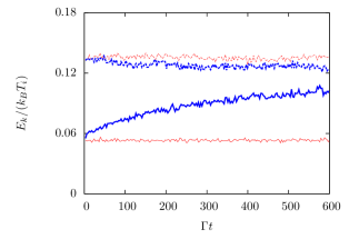
Figure 2: Time evolution of the mean energy of modes of wave vectors $k=0.3\sqrt{mg\rho_{i}}/\hbar$ (solid lines) and $k=6.0\sqrt{mg\rho_{i}}/\hbar$ (dashed lines), where $\rho_{i}$ is the initial density of each species, in the coupled (fat blue lines, $\tilde{g}=0.4g$) and uncoupled (thin red lines, $\tilde{g}=0$) cases. The loss process is turned off at time $t=2/\Gamma$ and shown is the subsequent evolution of the isolated system. The modes in the two uncoupled gases retain their respective energies after dissipation has been turned off to form a long-lived non-thermal state as above, while the modes in the coupled system relax towards an equipartition of energy. This highlights the role of integrability in the establishment of the long-lived non-thermal configuration. Here results are obtained by averaging over 10 samples, and for each sample we average the mode energy over a $k$ interval of 0.2$\sqrt{mg\rho_{i}}/\hbar$. The parameters of the simulation are: $T_{i}/(\rho_{i}\sqrt{\hbar g\rho_{i}/m})=0.04$, $m^{\prime}/m=3$ and $\hbar\Gamma/(\rho_{i}g)=4\times 10^{-3}$.

There are many ways to break the integrability of the system. In the model of two gases with different masses, the integrability is violently broken since a two particle collisional event does not preserve the set of momenta. A gentler way to break the integrability would be to consider two gases with atoms of the same mass, but with an interspecies coupling $\tilde{g}$ different from the intra-species coupling $g$. Here, any two-particle collision does preserve the set of momenta. This system is nevertheless non-integrable. However, our simulations of the classical field version of this system did not show any relaxation on the time scales shown in Fig (1).

Effect of quantum fluctuations associated with the atom-loss process— The above treatment does not take into account the quantized nature of the atomic field, i.e. the discreteness of the atoms. In particular, it ignores the shot noise in the loss process, which introduces additional heating and therefore limits the lowest attainable temperature. A description that accounts for the discreteness of the losses is provided by the stochastic Gross-Pitaevskii equation

$$i\hbar d\psi=\left(-\frac{\hbar^{2}}{2m}\frac{\partial^{2}}{\partial z^{2}}\psi+g|\psi|^{2}\psi-i\frac{\Gamma}{2}\psi\right)dt+d\xi,$$ (7)

where $\langle d\xi^{*}(z)d\xi(z^{\prime})\rangle=\Gamma dt\delta(z-z^{\prime})/2$. This equation can be derived by converting the master equation for the system density operator to a partial differential equation for the Wigner quasiprobability distribution. After the third- and higher-order derivatives associated with the nonlinear atomic interaction term are truncated (an uncontrolled approximation, but one that is typically valid for weakly-interacting Bose gases, provided the occupation per mode is not too small over the simulation timescale), evolution of the Wigner distribution takes the form of a Fokker-Planck equation, which can be efficiently simulated via Eq. (7). There exists a formal correspondence between the quantum field $\hat{\psi}(z)$ and $\psi(z)$: averaging over solutions to Eq. (7) correspond to symmetrically-ordered expectations (for more details see Appendix B; an alternative derivation is provided in Grišins et al. (2016)).

As shown in Appendix B, linearizing Eq. (7) in density fluctuations and phase gradient gives an independent evolution of each mode. Modes with frequencies much larger than the loss rate remain thermal, however their temperatures depend on the mode energy and have the following long-time behavior: $T_{\rm{phonon}}\underset{t\rightarrow\infty}{\simeq}\rho_{0}(t)g/k_{B}$ for phononic modes and $T_{\rm{part}}\underset{t\rightarrow\infty}{\simeq}\frac{\hbar^{2}k^{2}}{2m}\frac{1}{k_{B}\Gamma t}$ for particle modes. Note that, in contrast to pure classical field predictions, the temperature within the particle regime depends on $k$. Moreover, the ratio between $T_{\rm{part}}$ and $T_{\rm{phonon}}$,

$$\frac{T_{\rm{part}}}{T_{\rm{phonon}}}\underset{t\rightarrow\infty}{\simeq}\frac{k^{2}}{2g\rho_{i}}\frac{e^{\Gamma t}}{\Gamma t},$$ (8)

is much larger than the one predicted by a pure classical field theory. Thus, the effect of the shot noise associated with the discreteness of lost atoms amplifies the non-thermal nature of the state.

In order to test whether the above predictions including quantum noise are robust beyond the linearized approach, we numerically simulated the evolution given by Eq. (7). The initial thermal state, deep in the quasi-condensate regime, was sampled stochastically by using the linearized approach and taking into account quantum fluctuations (which is equivalent to sampling the Wigner function for a thermal state Sinatra et al. (2002); Olsen and Bradley (2009)). These samples were then evolved according to Eq. (7), and the energy $E_{k}$ of each Bogoliubov mode computed at each time (with averages over trajectories yielding $\langle E_{k}\rangle$ and the corresponding temperature $T_{k}=\hbar\omega_{k}/\{k_{B}\ln[(E_{k}+\hbar\omega_{k}/2)/(E_{k}-\hbar\omega_{k}/2)]\}$. Fig. 3 shows $T_{k}$ as a function of $k$ at three distinct times, and reveals that a non-thermal state is realized with a $k$-dependent temperature. At small $k$ we find, in agreement with the linearized approach, that the temperature converges towards $\rho_{0}(t)g$ at long times. At long times and large $k$, prediction fron Eq (8) are recovered.

Figure 3: Temperature of each mode, obtained from the stochastic Gross-Pitaevskii equation, as a function of the wavevector $k$ of the mode, for different evolution times : $\Gamma t=0$ (dotted green line), $\Gamma t=2.5$ (dashed blue line) and $\Gamma t=5.3$ (solid fat red line). The initial temperature is $k_{B}T_{i}/(\rho_{i}g)=3$. As atoms are lost, the gas is driven out of equilibrium and $T_{k}$ acquire a $k$-dependence. For phononic particles, we observe that $T_{k}$ tends towards $g\rho_{0}(t)$, as expected from the linearized approach. The smooth red solid line is the asymptotic result of Eq. (8), valid at long times for excitations in the particle regime, computed for $\Gamma t=5.3$. Parameters of the simulation are : $k_{B}T_{i}/(\hbar\rho_{i}\sqrt{g\rho_{i}/m})=3\times 10^{-3}$, $\hbar\Gamma/(g\rho_{i})=2\times 10^{-3}$ and $mg/(\hbar^{2}\rho_{i})=10^{-6}$.

Long-lived non-thermal states in harmonically-confined 1D gases — The generation of a state which is out-of-equilibrium raises concerns about experiments probing one-dimensional Bose gases, where this non-selective cooling scheme is expected to occur. In standard experiments, atoms are confined in a harmonic potential, which complicates the picture. To zeroth order in fluctuations, the density profile of the gas is given by the Thomas-Fermi inverted parabolic shape Pethick and Smith (2008) . At finite temperature, excitation modes above this Thomas-Fermi profile get populated. If the loss rate is sufficiently small, one expects that each mode adiabatically follows the changes of the Thomas-Fermi shape, such that each mode can be treated independently and, within the pure classical field approximation, Eq (3) is still valid, where $k$ is now a positive integer that indexes the mode. The frequency of phononic modes, i.e. modes of energy much smaller than the chemical potential $\mu$, are well approximated by $\omega_{k}=\nu\sqrt{k(k+1)/2}$, where $\nu$ is the harmonic trapping frequency Ho and Ma (1999). Thus, for modes which stay within the phonon regime during the entire loss process, Eq. (3) predicts that their temperature decreases as $e^{-\Gamma t}$.

The description of higher-energy modes, called particle modes, is not simple since they explore regions where the Thomas-Fermi density vanishes and the quasi-condensate approximation fails. It is reasonable however to believe that the energy spectrum at energies much larger than $\mu$ is close to the energy spectrum of free particles, so that frequencies of these modes are equally spaced, separated by $\nu$. Since the chemical potential decreases during the loss process, many excitations initially in the phononic regime are transferred to the particle regime. Let us consider such an excitation. Its frequency goes from $\omega_{k}\simeq k\nu/\sqrt{2}$ before the loss process , to about $k\nu$ at the end of the loss process when it lies in the particle regime. The ratio $\omega_{k}(t_{f})/\omega_{k}(0)$ is thus larger than one. According to the classical field prediction of Eq. (3), one therefore expects these excitations to attain a higher temperature than those lower excitations staying within the phonon regime.

The effect of shot noise on the loss process is not easy to treat for a trapped gas. However, we expect that, as in the case of a homogeneous gas, the quantum noise will amplify the non-thermal behavior of the system, so the temperature differences between modes could be even larger.

Experimental observation of a long-lived non-thermal state — Observing the non-thermal nature of the gas experimentally requires the ability to address modes of different energies independently. This is a priori not an easy task for gases confined in a box since all modes overlap spatially. However, since the atomic clouds in typical experiments are confined longitudinally in a slowly varying harmonic potential, there is some spatial separation of modes of different energy. At very low temperatures, thermal excitations of energy larger than $\rho_{p}g$ give the density profile ‘wings’ that extend beyond the Thomas-Fermi inverted parabola of peak density $\rho_{p}$. In contrast, low-energy excitations lying in the phononic regime do not extend beyond the Thomas-Fermi profile, but are responsible for long wavelength density fluctuations in the central region of the cloud. The density profile of the gas is thus most sensitive to high-energy excitations. Low-energy excitations, on the other hand, can be probed by investigating, within the Thomas-Fermi profile, atom-number fluctuations $\langle\delta N^{2}\rangle$, in pixels of length $\Delta$ much larger than the healing length $\xi_{0}$ Esteve et al. (2006).

Experimentally, we prepare clouds of ⁸⁷Rb atoms by radio-frequency evaporation in our atom-chip experiment, as described in  Armijo et al. (2011), and we record a set of density profiles taken under the same experimental conditions. The longitudinal trapping frequency is 6.2 Hz, while the transverse confinement is 1.9 kHz. Atoms are polarized in the $|F=2,m=2\rangle$ hyperfine ground state, where the interactions are characterized by the $s$-wave scattering length $a=5.2~{}nm$. Since the local density approximation is well fulfilled longitudinally, the equilibrium profile can be computed using the equation of state for longitudinally homogeneous gases, $\rho(\mu,T)$, where $\mu$ is the chemical potential. Using the well-established modified Yang-Yang equation of state van Amerongen et al. (2008); Armijo et al. (2011), where the effective 1D coupling constant is $g=2\hbar\omega_{\perp}a$, the experimental density profile is fitted for a temperature $T_{pr}=140~{}$nK (see Fig. 4). We also extract atom-number fluctuations $\langle\delta N^{2}\rangle$ in each pixel from the same dataset, giving an independent temperature measurement. Since $\Delta$ is both much smaller than the cloud size and much larger than the healing length, the physics of homogeneous gases is locally probed and thermodynamics predicts $\langle\delta N^{2}\rangle=k_{B}T\Delta\partial\rho/\partial\mu$ Armijo et al. (2011). In Fig. 4, we plot $\langle\delta N^{2}\rangle$ versus the mean atom number in the pixel. Fitting the large atom-number region, corresponding to pixels lying inside the Thomas-Fermi profile, with the fluctuation-dissipation relation and the quasi-condensate equation of state, we extract a temperature $T_{\text{fl}}=80$ nK (as summarized in Fig. 4). The difference between $T_{\text{pr}}$ and $T_{\text{fl}}$ is a signature that the cloud is out-of-equilibrium. We also confirmed that, after the radio-frequency loss mechanism has been removed, this situation is stable over the cloud lifetime of about one second (Fig. 4). Since the profile is more sensitive to high-energy excitations while the density fluctuations are more sensitive to low energy excitations, the fact that $T_{\text{pr}}>T_{\text{fl}}$ could be related to the above quantitative study of homogeneous gases and the qualitative arguments given for the trapped system. In the experiments presented in Rauer et al. (2016), only low-energy excitations were probed and consequently this non-thermal character was not revealed.

Figure 4: Results of the two thermometries we performed on the experiment. (a) Atom number fluctuations. Fitting the central region of the cloud, i.e. the high atom-number part, (red line) gives a first temperature $T_{fl}=80$ nK. However, the expected profile from this temperature (also the red curve on (b)) lies well below the experimental data. A second temperature $T_{pr}=140$ nK is found by fitting the profile with the equation of state (solid green line). By plotting the expected atom number fluctuations from $T_{pr}$ on (a), the prediction is in good agreement with the small atom number region. That is, the center of the cloud appears to be at a different temperature than the edges. The close to 50% discrepancy is well beyond the uncertainty we have on the temperature measurements, which is around 10 %.(c) Data showing that this temperature difference is stationary over time: we observed a long-lived non-thermal state.

To conclude, we theoretically investigated the long-lived non-thermal state produced by the non-selective removal of atoms in order to cool a uniform one-dimensional Bose gas. This dissipation drives the system out-of-equilibrium, with different excitation modes losing energies at different rates. This out-of-equilibrium character is robust against coupling between modes introduced in the Gross-Pitaevskii equation, and is related to the integrable nature of the considered system. We performed simulations of a two-species Bose mixture with different masses, a non-integrable system, and confirmed a slow relaxation towards an equipartition of energy between excitations. Truncated Wigner simulations that go beyond the pure classical-field description and include the shot-noise associated to the loss process due to the quantized nature of the atomic field further confirmed the non-thermal nature of the state produced by dissipation. Finally, we discussed the relevance of our findings for experimental realizations of 1D Bose gases trapped in a harmonic potential. From a theoretical point of view, in the linearized classical field approach, a small temperature difference between modes of different energies is indeed expected, and this effect could be amplified by the presence of quantum noise. In our quasi-condensate experiments, we indeed have signatures of a non-thermal character since different thermometries that probe different parts of the excitation spectrum give substantially different temperatures. However, a more careful and quantitative description in the trap, perhaps via finite-temperature classical field simulations Blakie et al. (2008), is still required in order to draw firm conclusions on the relation between these experimental long-lived non-thermal states and our theoretical findings.

Acknowledgements — We acknowledge fruitful discussions with M. J. Davis, K. V. Kheruntsyan, and M. Olshanii. This work has been supported by Cnano IdF. S.S.S. acknowledges support from the Australian Research Council (ARC) Centre of Excellence for Engineered Quantum Systems (Grant No. CE110001013) and the ARC Discovery Project Grant No. DP160103311.

Appendix A Breaking integrability : two coupled 1D Bose gases

An example of a non-integrable system is two quasi-condensates of different masses $m$ and $m^{\prime}$ oupled via an interaction term of coupling constant $\tilde{g}$. Here integrability is broken by two-body collisions involving an atom of each species, which does not preserve the set of two initial momenta. Within the classical field approximation, this system is described by the Hamiltonian

$$\begin{array}[]{ll}H=&\int dz\frac{\hbar^{2}}{2m}\left|\frac{\partial\psi}{\partial z}\right|^{2}+\int dz\frac{\hbar^{2}}{2m^{\prime}}\left|\frac{\partial\varphi}{\partial z}\right|^{2}\\ &+\frac{g}{2}\int dz|\psi(z)|^{4}+\frac{g}{2}\int dz|\varphi(z)|^{4}\\ &+\tilde{g}\int dz|\psi(z)|^{2}|\varphi(z)|^{2}\end{array}$$ (9)

which yields the equations of motion Eqs. (6). Within the density/phase representation, we can write $\psi=\sqrt{\rho}e^{i\theta}$ and $\varphi=\sqrt{\tilde{\rho}}e^{i\tilde{\theta}}$. For sufficiently low temperatures, the repulsive interactions result in very small density fluctuations and long wavelength phase fluctuations, such that one can linearize the equations of motion in $\delta\rho$, $\delta\tilde{\rho}$, $\partial\theta/\partial z$ and $\partial\tilde{\theta}/\partial z$, or equivalently retain only second-order terms in the Hamiltonian, which can then be diagonalized using a standard Bogoliubov procedure. We give more details on this approach below.

Since Eqs. (6) do not explicitly depend on $z$, different Fourier components evolve independently of each other. Let us consider the Fourier components of wave vector $k=2n\pi/L$ where $n$ is a positive integer and $L$ is the length of the box that confines the gases. As for the single component case, we introduce Fourier coefficients $\delta\rho_{ck}=\sqrt{2/L}\int dz\delta\rho(z)\cos(kz)$, and $\delta{\rho}_{sk}=\sqrt{2/L}\int dz\delta\rho(z)\sin(kz)$, and similarly for $\delta\tilde{\rho}$, $\theta$ and $\tilde{\theta}_{2}$. Each mode $jk$ evolves independently according to the quadratic Hamiltonian

$$\begin{array}[]{ll}H_{jk}=&(\frac{g}{2}+\frac{\hbar^{2}k^{2}}{8m\rho_{0}})\delta{\rho}_{jk}^{2}+\frac{\hbar^{2}k^{2}\rho_{0}}{2m}{\theta}_{jk}^{2}\\ &+(\frac{g}{2}+\frac{\hbar^{2}k^{2}}{8m^{\prime}\rho_{0}})\delta{\tilde{\rho}}_{jk}^{2}+\frac{\hbar^{2}k^{2}\rho_{0}}{2m^{\prime}}{\tilde{\theta}}_{jk}^{2}\\ &+\tilde{g}\delta{\rho}_{jk}\delta{\tilde{\rho}}_{jk},\end{array}$$ (10)

where $j=c$ or $s$. This gives the following linearized equation of motion

$$i\hbar\frac{\partial}{\partial t}\left(\begin{array}[]{l}2\sqrt{\rho_{0}}{\theta}_{jk}\\ \delta{\rho}_{jk}/\sqrt{\rho_{0}}\\ 2\sqrt{\rho_{0}}{\tilde{\theta}}_{jk}\\ \delta{\tilde{\rho}}_{jk}/\sqrt{\rho_{0}}\\ \end{array}\right)={\cal L}\left(\begin{array}[]{l}2\sqrt{\rho_{0}}{\theta}_{jk}\\ \delta{\rho}_{jk}/\sqrt{\rho_{0}}\\ 2\sqrt{\rho_{0}}{\tilde{\theta}}_{jk}\\ \delta{\tilde{\rho}}_{jk}/\sqrt{\rho_{0}}\\ \end{array}\right)$$ (11)

where

$${\cal L}=i\left(\begin{array}[]{cccc}0&2\rho_{0}g+\frac{\hbar^{2}k^{2}}{2m}&0&2\tilde{g}\rho_{0}\\ -\frac{\hbar^{2}k^{2}}{2m}&0&0&0\\ 0&2\tilde{g}\rho_{0}&0&2\rho_{0}g+\frac{\hbar^{2}k^{2}}{2m^{\prime}}\\ 0&0&-\frac{\hbar^{2}k^{2}}{2m^{\prime}}&0\end{array}\right).$$ (12)

Symmetry properties of ${\cal L}$ show that this operator has two eigenvectors

$${\cal L}\left(\begin{array}[]{c}F_{1}^{+}\\ iF_{1}^{-}\\ F_{2}^{+}\\ iF_{2}^{-}\\ \end{array}\right)=\omega_{a}\left(\begin{array}[]{c}F_{1}^{+}\\ iF_{1}^{-}\\ F_{2}^{+}\\ iF_{2}^{-}\\ \end{array}\right)$$ (13)

and

$${\cal L}\left(\begin{array}[]{c}G_{1}^{+}\\ iG_{1}^{-}\\ G_{2}^{+}\\ iG_{2}^{-}\\ \end{array}\right)=\omega_{b}\left(\begin{array}[]{c}G_{1}^{+}\\ iG_{1}^{-}\\ G_{2}^{+}\\ iG_{2}^{-}\\ \end{array}\right)$$ (14)

where, $F_{1}^{+},F_{1}^{-},F_{2}^{+},F_{2}^{-},G_{1}^{+},G_{1}^{-},G_{2}^{+},G_{2}^{-}$ are real and satisfy the normalisation condition

$$\left\{\begin{array}[]{l}G_{1}^{-}G_{1}^{+}+G_{2}^{-}G_{2}^{+}=1\\ F_{1}^{-}F_{1}^{+}+F_{2}^{-}F_{2}^{+}=1.\end{array}\right.$$ (15)

The vectors $(F_{1}^{+},-iF_{1}^{-},F_{2}^{+},-iF_{2}^{-})^{T}$ and $(G_{1}^{+},-iG_{1}^{-},G_{2}^{+},-iG_{2}^{-})^{T}$ are eigenvectors of ${\cal L}$ of eigenergies $-\omega_{a}$ and $-\omega_{b}$ respectively, which complete the basis. Expanding the state $(2\sqrt{\rho_{0}}{\theta}_{jk},\delta{\rho}_{jk}/\sqrt{\rho_{0}},2\sqrt{\rho_{0}}{\tilde{\theta}}_{jk},\delta{\tilde{\rho}}_{jk}/\sqrt{\rho_{0}})^{\top}$ on these the eigenbasis of ${\cal L}$ gives

$$\left\{\begin{array}[]{lll}2\sqrt{\rho_{0}}{\theta}_{jk}&=&-F_{1}^{+}i(a-a^{*})-G_{1}^{+}i(b-b^{*})\\ \delta{\rho}_{jk}/\sqrt{\rho_{0}}&=&F_{1}^{-}(a+a^{*})+G_{1}^{-}(b+b^{*})\\ 2\sqrt{\rho_{0}}{\tilde{\theta}}_{jk}&=&-F_{2}^{+}i(a-a^{*})-G_{2}^{+}i(b-b^{*})\\ \delta{\tilde{\rho}}_{jk}/\sqrt{\rho_{0}}&=&F_{2}^{-}(a+a^{*})+G_{2}^{-}(b+b^{*})\\ \\ \end{array}\right.$$ (16)

where $a$ and $b$ are c-numbers satisfying

$$i\hbar\partial a/\partial t =\hbar\omega_{a}a,$$ (17a)

$$i\hbar\partial b/\partial t =\hbar\omega_{b}b.$$ (17b)

Inserting into Eq. (10), we find that the Hamiltonian $H_{jk}$ can be written as:

$$H_{jk}=\hbar\omega_{a}|a|^{2}+\hbar\omega_{b}|b|^{2}$$ (18)

Although the above procedure utilizes the classical field approach, a quantum version yields similar results, with $a$ and $b$ replaced by bosonic operators and $\hat{H}_{jk}=E_{k}^{0}+\hbar\omega_{a}\hat{a}^{\dagger}\hat{a}+\hbar\omega_{b}\hat{b}^{\dagger}\hat{b}$, where $E_{k}^{0}$ is the contribution of the modes $a$ and $b$ to the vaccuum energy.

We use the linearization above to sample the initial state according to a thermal distribution. For this purpose, for each $jk$ Fourier component, we diagonalize ${\cal L}$ and we then sample the c-number $a$ and $b$ according to the thermal Gaussian law $k_{B}T=\hbar\omega_{a}\langle|a|^{2}\rangle$ and $k_{B}T=\hbar\omega_{b}\langle|b|^{2}\rangle$. From this, we can compute the fields $\psi$ and $\varphi$, subsequently evolve according to Eqs. (6), and extract the energy $H_{jk}$ of each Fourier component at each time point.

Appendix B Stochastic Gross-Pitaevskii equation

B.1 Derivation via truncated Wigner

Here we present a derivation of Eq. (7) from a Wigner distribution formalism and the truncated Wigner approximation. This methodology has had great success in the numerical modelling of weakly-interacting Bose gases in regimes where quantum fluctuations are important Drummond and Hardman (1993); Carter (1995); Steel et al. (1998); Polkovnikov (2010), and furthermore underpins the classical field methodology used for both zero and finite temperature simulations Blakie et al. (2008). Since the Bose gas is described by a quantum field, the derivation should strictly rely upon functional calculus (for details see, for example, Opanchuk and Drummond (2013)). However, since we are primarily concerned with numerical simulation on discrete grids with a finite number of points, for simplicity of presentation we will discretize the problem. That is, we divide space into cells of length $\delta x$, and discretize the field operator such that $\hat{\psi}_{r}$ annihilates an atom in the cell $r$, and satisfies $[\hat{\psi}^{\dagger}_{r},\hat{\psi}_{r^{\prime}}]=\delta_{r,r^{\prime}}$. Furthermore, we introduce the per-cell interaction energy $\tilde{g}=g/\delta x$ and the operator $\partial_{r}^{2}\equiv\partial^{2}/\partial_{r}^{2}$, which must be interpreted as $\partial_{r}^{2}\left.\{f\}\right|_{r}=(f_{r+1}+f_{r-1}-2f_{r})/\delta x^{2}$ when applied to a discrete function $f_{r}$, where integer $r$ indexes the cell.

A homogeneous 1D Bose gas undergoing a non-selective loss process can be described by the master equation

$$\frac{\partial\rho}{\partial t}=-\frac{i}{\hbar}[\hat{H},\rho]+\Gamma\sum_{r}\mathcal{D}[\hat{\psi}_{r}]\rho,$$ (19)

where $\rho$ is the system density operator, $\mathcal{D}[\hat{L}]\rho\equiv\hat{L}\rho\hat{L}^{\dagger}-\tfrac{1}{2}\hat{L}^{\dagger}\hat{L}\rho-\tfrac{1}{2}\rho\hat{L}^{\dagger}\hat{L}$, and $\hat{H}$ is the Lieb-Liniger Hamiltonian

$$\hat{H}=\sum_{r}\left(-\hat{\psi}_{r}^{\dagger}\frac{\hbar^{2}}{2m}\partial_{r}^{2}\hat{\psi}_{r}+\frac{\tilde{g}}{2}\hat{\psi}_{r}^{\dagger}\hat{\psi}_{r}^{\dagger}\psi_{r}\psi_{r}\right).$$ (20)

The system density operator can be equivalently described by the Wigner quasiprobability distribution, $W$, which is a real function of a complex field ${\psi(z)}$ :

$$W(\left\{\psi_{r},\psi_{r}^{*}\right\})=\int\prod_{r}d^{2}\lambda_{r}\frac{e^{-(\lambda_{r}\psi^{*}_{r}+\lambda^{*}_{r}\psi_{r})}}{\pi^{2}}\chi(\left\{\lambda_{r},\lambda_{r}^{*}\right\}),$$ (21)

where $\chi(\left\{\lambda_{r},\lambda_{r}^{*}\right\})$ is the characteristic function

$$\chi(\left\{\lambda_{r},\lambda_{r}^{*}\right\})=\text{Tr}\left\{\rho\exp\left[\sum_{r}(\lambda_{r}\hat{\psi}_{r}^{\dagger}-\lambda_{r}^{*}\hat{\psi}_{r})\right]\right\}.$$ (22)

Averages of functions of $\psi_{r},\psi_{r}^{*}$ over $W$ correspond to expectations of the corresponding symmetrically-ordered operators. Using the operator correspondences Blakie et al. (2008); Opanchuk and Drummond (2013)

$$\hat{\psi}_{r}\rho\to\left(\psi_{r}+\frac{1}{2}\frac{\partial}{\partial\psi_{r}^{*}}\right)W(\left\{\psi_{r},\psi_{r}^{*}\right\}),$$ (23a)

$$\hat{\psi}_{r}^{\dagger}\rho\to\left(\psi_{r}^{*}-\frac{1}{2}\frac{\partial}{\partial\psi_{r}}\right)W(\left\{\psi_{r},\psi_{r}^{*}\right\}),$$ (23b)

$$\rho\hat{\psi}_{r}\to\left(\psi_{r}-\frac{1}{2}\frac{\partial}{\partial\psi_{r}^{*}}\right)W(\left\{\psi_{r},\psi_{r}^{*}\right\}),$$ (23c)

$$\rho\hat{\psi}_{r}^{\dagger}\to\left(\psi_{r}^{*}+\frac{1}{2}\frac{\partial}{\partial\psi_{r}}\right)W(\left\{\psi_{r},\psi_{r}^{*}\right\}),$$ (23d)

we can map the master equation Eq. (19) to the following partial differential equation for the Wigner function:

$$\frac{\partial W}{\partial t}=\frac{\partial W}{\partial t}\Big{|}_{\text{Kin}}+\frac{\partial W}{\partial t}\Big{|}_{\text{Nonlin}}+\frac{\partial W}{\partial t}\Big{|}_{\text{Loss}}$$ (24)

where

$$\frac{\partial W}{\partial t}\Big{|}_{\text{Kin}} =\frac{i\hbar}{2m}\sum_{r}\left\{\frac{\partial}{\partial\psi_{r}}\partial_{r}^{2}\psi_{r}-\frac{\partial}{\partial\psi_{r}^{*}}\partial_{r}^{2}\psi_{r}^{*}\right\}W$$ (25)

corresponds to the kinetic energy term,

$$\frac{\partial W}{\partial t}\Big{|}_{\text{Nonlin}}=\frac{i\tilde{g}}{\hbar}\sum_{r}\Bigg{\{}\frac{1}{4}\left(\frac{\partial^{3}}{\partial^{2}\psi_{r}\partial\psi_{r}^{*}}\psi_{r}-\frac{\partial^{3}}{\partial^{2}\psi_{r}^{*}\partial\psi_{r}}\psi_{r}^{*}\right)\\ +\left(\frac{\partial}{\partial\psi_{r}}\psi_{r}-\frac{\partial}{\partial\psi_{r}^{*}}\psi_{r}^{*}\right)(|\psi_{r}|^{2}-1)\Bigg{\}}W,$$ (26)

corresponds to the nonlinear atom-atom collisional term, and

$$\frac{\partial W}{\partial t}\Big{|}_{\text{Loss}} =\frac{\Gamma}{2}\sum_{r}\left\{-\frac{\partial}{\partial\psi_{r}}\psi_{r}+\frac{\partial}{\partial\psi^{*}_{r}}\psi^{*}_{r}+\frac{\partial^{2}}{\partial\psi_{r}\partial\psi_{r}^{*}}\right\}W$$ (27)

corresponds to the loss term. This is currently no easier to simulate than the master equation Eq. (19). However, if we truncate the third-order derivatives in term Eq. (26) that arise due to the nonlinearity, then Eq. (24) takes the form of a Fokker-Planck equation with positive definite diffusion. It can therefore be efficiently simulated via a set of stochastic differential equations. One can replacing $(|\psi|^{2}-1)$ in equation (26) by $|\psi|^{2}$ since this corresponds to a simple, irrelevant, energy shift. We then find that the differential equations are just the the stochastic Gross-Pitaevskii equation, Eq. (7). The truncation of these third-order derivatives is an uncontrolled approximation, but is typically valid for weakly-interacting Bose gases, provided the occupation per mode is not too small over the simulation timescale. Note that the truncated Wigner approximation applied here concerns the treatment of interactions between atoms in the quasi-condensate. The sole effect of losses is captured in a exact way by this procedure at the quantum level.

B.2 Linearized approach

In the quasicondensate regime density fluctuations and phase gradients are small. A linearized approach can therefore be used to identify independent modes, following the procedure below. Separating the real and imaginary parts of Eq. (7) and linearizing in density fluctuations and the phase gradient gives the stochastic equations

$$\left\{\begin{array}[]{l}d\delta\rho_{r}=-\frac{\hbar^{2}\rho_{0}}{m}\partial_{r}^{2}\theta dt-\Gamma\delta\rho_{r}dt+\sqrt{\rho_{0}}d\eta_{r}\\ d\theta_{r}=-(\tilde{g}-\frac{\hbar^{2}}{4m\rho_{0}}\partial_{r}^{2})\delta\rho_{r}dt+\frac{1}{2\sqrt{\rho_{0}}}d\nu_{r}\end{array}\right.$$ (28)

where $d\nu_{r}$ and $d\eta_{r}$ are random Gaussian variables with zero mean and variances $\langle d\eta_{r}d\eta_{r^{\prime}}\rangle=\langle d\nu_{r}d\nu_{r^{\prime}}\rangle=\delta_{r,r^{\prime}}\Gamma dt$. Expanding $\theta_{r}$ and $\delta\rho_{r}$ on sinusoidal modes, $\theta=\sum_{k>0}\sqrt{2/L}[\theta_{ck}\cos(kz)+\theta_{sk}\sin(kz)]$ and $\delta\rho=\sum_{k>0}\sqrt{2/L}[\delta\rho_{ck}\cos(kz)+\delta\rho_{sk}\sin(kz)]$ gives

$$\left\{\begin{array}[]{l}d\delta\rho_{jk}=\frac{\hbar^{2}k^{2}\rho_{0}}{m}\theta_{jk}dt-\Gamma\delta\rho_{jk}dt+\sqrt{\rho_{0}}d\eta_{jk},\\ d\theta_{jk}=-(\tilde{g}-\frac{\hbar^{2}k^{2}}{4m\rho_{0}})\delta\rho_{jk}dt+\frac{1}{2\sqrt{\rho_{0}}}d\nu_{jk},\end{array}\right.$$ (29)

where $d\nu_{jk}$ and $d\eta_{jk}$ are random Gaussian variables of vanishing mean and variances $\langle d\eta_{jk}^{2}\rangle=\langle d\nu_{jk}^{2}\rangle=\Gamma dt$. An initial centered Gaussian Wigner distribution (such as a thermal state) remains Gaussian under the above linearized stochastic evolution. Moreover, after averaging over stochastic trajectories, it remains centered on $\langle\delta\rho_{jk}\rangle=\langle\theta_{jk}\rangle=0$. Consequently the Wigner distribution for each mode is entirely determined by variances and covariances of the variables - explicitly, entirely determined by the following coupled differential equations:

$$\left\{\begin{array}[]{l}\frac{d}{dt}\langle\delta\rho_{jk}^{2}\rangle=2\frac{\hbar^{2}k^{2}\rho_{0}}{m}\langle\theta_{jk}\delta\rho_{jk}\rangle-2\Gamma\langle\delta\rho_{jk}^{2}\rangle+\rho_{0}\Gamma\\ \frac{d}{dt}\langle\theta_{jk}^{2}\rangle=-2(\tilde{g}-\frac{\hbar^{2}k^{2}}{4m\rho_{0}})\langle\theta_{k,j}\delta\rho_{jk}\rangle+\frac{\Gamma}{4\rho_{0}}\\ \frac{d}{dt}\langle\delta\rho_{jk}\theta_{jk}\rangle=\frac{\hbar^{2}k^{2}\rho_{0}}{m}\langle\theta_{jk}^{2}\rangle-(\tilde{g}-\frac{\hbar^{2}k^{2}}{4m\rho_{0}})\langle\theta_{jk}^{2}\rangle\end{array}\right.$$ (30)

The link between these classical averages over $\delta\rho_{jk}$ and $\delta\theta_{jk}$ and the expectations over the corresponding quantum operators is not immediate. Strictly, averages over various combinations of the $c$-number fields $\psi_{r}$ and $\psi_{r}^{*}$ correspond to expectations of symmetric orderings of the corresponding quantum operators - for example

$$\langle(\hat{\psi}_{r^{\prime}}^{\dagger}\hat{\psi}_{r}+\hat{\psi}_{r}\psi_{r^{\prime}}^{\dagger})/2\rangle=\overline{\psi_{r^{\prime}}^{*}\psi_{r}}.$$

However, since in the quasi-condensate regime correlation lengths are much larger than the mean inter-particle distance and density fluctuations are small, one can use a coarse-grained approximation where the atom number in each cell is large yielding small relative fluctuations. Then the atomic density $\langle\hat{\psi}_{r}^{\dagger}\hat{\psi}_{r}\rangle$ and its higher-order moments are well-approximated simply by classical averages over $\psi^{*}\psi$ and its powers. Put another way, those corrections that arise due to the non-commutativity of the operators are small and can be neglected. A similar argument holds for the phase operator. Consequently, we are justified in interpreting those classical averages within Eqs. (30) as quantum expectations.

Let us focus on the evolution of a given mode of wavevector $k$ and assume the loss rate is very small compared to the mode frequency $\omega_{k}=\sqrt{\hbar^{2}k^{2}/(2m)(\hbar^{2}k^{2}/(2m)+2\tilde{g}\rho_{0})}$. Then, the free evolution ensures equipartition of the energy between the two conjugate variables $\delta\rho_{jk}$ and $\theta_{jk}$ at any time, which corresponds to thermal equilibrium. The Wigner function is then solely determined by the mean energy in the mode $E_{k}$ and one finds, from Eq. (30),

$$\frac{d}{dt}\tilde{E}=\Gamma\left(-\tilde{E}+(\bar{A}_{k}^{2}+1/\bar{A}_{k}^{2})/4\right)$$ (31)

where $\bar{A}_{k}=[(\hbar^{2}k^{2}/(2m)+2g\rho_{0})/(\hbar^{2}k^{2}/(2m))]^{1/4}$ and $\tilde{E}=E_{k}/\omega_{k}$. For phonons, $\bar{A}_{k}\approx[4mg\rho_{0}/(\hbar^{2}k^{2})]^{1/4}$ and is much larger than 1. Using this time-dependant approximation of $A_{k}$ to solve Eq. (31), we find that $E_{k}$ asymptotically goes towards $g\rho_{0}(t)$. Since $g\rho_{0}(t)$ is much larger than the ground state energy for phonons, the Rayleigh-Jeans limit is attained, and this corresponds to a thermal equilibrium at temperature

$$k_{B}T_{\rm{phonon}}\underset{t\rightarrow\infty}{\simeq}\rho_{0}(t)g.$$ (32)

In contrast, for modes with $k\gg\sqrt{\rho_{0}g}$, an expansion of $\bar{A}_{k}$ in power of $g\rho_{0}/(\hbar^{2}k^{2}/m)$, one finds

$$\tilde{\epsilon}\simeq\left(\frac{mg\rho_{0}}{\hbar^{2}k^{2}}\right)^{2}e^{-\Gamma t}(1-e^{-\Gamma t})+\tilde{\epsilon}_{0}e^{-\Gamma t}$$ (33)

where $\tilde{\epsilon}=(\tilde{E}-1/2)/\omega_{k}$ is the mean quantum occupation number of the mode. At large times, $\tilde{\epsilon}$ becomes much smaller than one. This corresponds to a temperature $k_{B}T\simeq-(\hbar^{2}k^{2}/(2m))\ln(\tilde{\epsilon})$, much smaller than $\omega_{k}$. At large times, we find

$$k_{B}T_{\rm{part}}\underset{t\rightarrow\infty}{\simeq}\frac{\hbar^{2}k^{2}}{2m}\frac{1}{\Gamma t}.$$ (34)

The temperature of those modes depends on $k$ and takes much larger values than $T_{\rm{phonon}}$.

Finally, note that, while in this appendix we start from the truncated Wigner stochastic equation to derive the above linearized approach, an alternative approach is to linearize the Lieb-Liniger Hamiltonian and then consider, for a given mode, the effect of losses. Thus, the validity of linearized approach does not require that the mode occupation number be large. It is valid even in the quantum regime, the approximation here being that the gas lies deeply enough in the quasi-condensate regime.

References

- Luiten et al. (1996) O. J. Luiten, M. W. Reynolds, and J. T. M. Walraven, Physical Review A 53, 381 (1996).
- Hofferberth et al. (2008) S. Hofferberth, I. Lesanovsky, T. Schumm, A. Imambekov, V. Gritsev, E. Demler, and J. Schmiedmayer, Nat Phys 4, 489 (2008).
- Jacqmin et al. (2011) T. Jacqmin, J. Armijo, T. Berrada, K. V. Kheruntsyan, and I. Bouchoule, Phys. Rev. Lett. 106, 230405 (2011).
- Kheruntsyan et al. (2003) K. Kheruntsyan, D. Gangardt, P. Drummond, and G. Shlyapnikov, Phys. Rev. Lett. 91, 040403 (2003).
- Bloch et al. (2006) I. Bloch, J. Dalibard, and W. Zwerger, Rev. Mod.Phys. 80, 885 (2006).
- Grišins et al. (2016) P. Grišins, B. Rauer, T. Langen, J. Schmiedmayer, and I. E. Mazets, Phys. Rev. A 93, 033634 (2016).
- Rauer et al. (2016) B. Rauer, P. Grišins, I. Mazets, T. Schweigler, W. Rohringer, R. Geiger, T. Langen, and J. Schmiedmayer, Phys. Rev. Lett. 116, 030402 (2016).
- Deutsch (1991) J. M. Deutsch, Phys. Rev. A 43, 2046 (1991).
- Rigol et al. (2008) M. Rigol, V. Dunjko, and M. Olshanii, Nature 452, 854 (2008).
- Fang et al. (2014) B. Fang, G. Carleo, A. Johnson, and I. Bouchoule, Phys. Rev. Lett. 113, 035301 (2014).
- Fang et al. (2016) B. Fang, A. Johnson, T. Roscilde, and I. Bouchoule, Phys. Rev. Lett. 116, 050402 (2016).
- Wade et al. (2016) A. C. J. Wade, J. F. Sherson, and K. Mølmer, Phys. Rev. A 93, 023610 (2016).
- Langen et al. (2015) T. Langen, S. Erne, R. Geiger, B. Rauer, T. Schweigler, M. Kuhnert, W. Rohringer, I. E. Mazets, T. Gasenzer, and J. Schmiedmayer, Science 348, 207 (2015).
- Kulkarni and Lamacraft (2013) M. Kulkarni and A. Lamacraft, Phys. Rev. A 88, 021603 (2013).
- Mazets and Schmiedmayer (2009) I. E. Mazets and J. Schmiedmayer, Eur. Phys. J. B 68, 335 (2009).
- Castin et al. (2000) Y. Castin, R. Dum, E. Mandonnet, A. Minguzzi, and I. Carusotto, Journal of Modern Optics 47, 2671 (2000).
- Bouchoule et al. (2016) I. Bouchoule, S. S. Szigeti, M. J. Davis, and K. V. Kheruntsyan, Phys. Rev. A 94, 051602 (2016).
- Grisins and Mazets (2011) P. Grisins and I. E. Mazets, Phys. Rev. A 84, 053635 (2011).
- Sinatra et al. (2002) A. Sinatra, C. Lobo, and Y. Castin, Journal of Physics B: Atomic, Molecular and Optical Physics 35, 3599 (2002).
- Olsen and Bradley (2009) M. Olsen and A. Bradley, Optics Communications 282, 3924 (2009).
- Pethick and Smith (2008) C. J. Pethick and H. Smith, Bose–Einstein Condensation in Dilute Gases:, 2nd ed. (Cambridge University Press, Cambridge, 2008).
- Note (1) We assume here the trapping frequency is much smaller than , where is the central atomic density.
- Ho and Ma (1999) T.-L. Ho and M. Ma, Journal of Low Temperature Physics 115, 61 (1999).
- Note (2) We assume here .
- Esteve et al. (2006) J. Esteve, J.-B. Trebbia, T. Schumm, A. Aspect, C. I. Westbrook, and I. Bouchoule, Phys. Rev. Lett. 96, 130403 (2006).
- Armijo et al. (2011) J. Armijo, T. Jacqmin, K. Kheruntsyan, and I. Bouchoule, Phys. Rev. A 83, 021605 (2011).
- van Amerongen et al. (2008) A. H. van Amerongen, J. J. P. van Es, P. Wicke, K. V. Kheruntsyan, and N. J. van Druten, Phys. Rev. Lett. 100, 090402 (2008).
- Blakie et al. (2008) P. B. Blakie, A. S. Bradley, M. J. Davis, R. J. Ballagh, and C. W. Gardiner, Advances in Physics, Advances in Physics 57, 363 (2008).
- Drummond and Hardman (1993) P. D. Drummond and A. D. Hardman, EPL (Europhysics Letters) 21, 279 (1993).
- Carter (1995) S. J. Carter, Phys. Rev. A 51, 3274 (1995).
- Steel et al. (1998) M. J. Steel, M. K. Olsen, L. I. Plimak, P. D. Drummond, S. M. Tan, M. J. Collett, D. F. Walls, and R. Graham, Phys. Rev. A 58, 4824 (1998).
- Polkovnikov (2010) A. Polkovnikov, Annals of Physics 325, 1790 (2010).
- Opanchuk and Drummond (2013) B. Opanchuk and P. D. Drummond, Journal of Mathematical Physics 54, 042107 (2013).