Grand Unified Brane World Scenario

Abstract

We present a field theoretical model unifying grand unified theory (GUT) and brane world scenario. As a concrete example, we consider $SU(5)$ GUT in 4+1 dimensions where our $3+1$ dimensional spacetime spontaneously arises on five domain walls. A field-dependent gauge kinetic term is used to localize massless non-Abelian gauge fields on the domain walls and to assure the charge universality of matter fields. We find the domain walls with the symmetry breaking $SU(5)\to SU(3)\times SU(2)\times U(1)$ as a global minimum and all the undesirable moduli are stabilized with the mass scale of $M_{\rm GUT}$. Profiles of massless Standard Model particles are determined as a consequence of wall dynamics. The proton decay can be exponentially suppressed.

I Introduction

Grand unified theories (GUT) Pati:1973uk ; Georgi:1974sy ; Georgi:1974yf ; Witten:1981nf ; Dimopoulos:1981zb ; Sakai:1981gr ; Dimopoulos:1981yj have various interesting features such as prediction of gauge coupling unification and explanation of the charge assignments of matters. Theories with extra-dimensions give a solution of the gauge hierarchy problem in the framework such as the brane world scenario ArkaniHamed:1998rs ; Antoniadis:1998ig ; RS ; RS2 ; Akama . Combining these two theories gives rise to new possibilities for phenomenological model building.

An interesting example is $SU(5)$ GUT in five dimensional space-time where the fifth dimension is compactified on an orbifold Kawamura:1999nj . In this kind of model, several assumptions are made: i) The fifth dimension is compactifed. ii) Two branes exist. iii) Matter fields are localized on one of two branes called an Infra-Red brane while gauge fields and Higgs fields propagate in the bulk. iv) Nontrivial $\mathbf{Z}_{2}$ parity assignment for the fields is required. This setup leads to breaking of $SU(5)$ gauge group to the Standard Model (SM) gauge group and realizes chiral fermions on the Infra-Red brane. Further studies along this direction have been done to reconsider traditional problems in GUT such as doublet-triplet Higgs splitting and proton decay which has not been observed so far Kawamura:2000ev ; Kawamura:2000ir ; Altarelli:2001qj ; Hall:2001pg ; Hebecker:2001wq . A key feature in these models is gauge symmetry breaking via orbifold compactification. However, the origins of the nontrivial space-time geometry (only the fifth direction is compact) and the $\mathbf{Z}_{2}$ parity assignment has not been explained. Moreover, both the presence of infinitely thin branes and the localization of matters on an Infra-Red brane are assumed as an initial setup.

These points, however, can be addressed in non-compact five dimensional space-time. A minimal assumption is a presence of discrete vacua which are exchanged by a discrete symmetry. Spontaneous symmetry breaking of the discrete symmetry dynamically yields stable domain walls, which are solutions of equations of motion. Thus, our four-dimensional world is dynamically realized as the domain walls with finite width in flat 5 dimensional spacetime. Furthermore, they automatically lead to localization of zero modes of matter fields in the bulk such as fermions and scalars Rubakov . It provides a dynamical realization of four-dimensional space-time, namely, the brane world scenario.

An $SU(5)$ GUT model in the five-dimensional space-time with a domain wall background has been proposed in Ref. Volkas , and has been studied extensively in Davidson:2007cf ; Volkas2 ; Callen:2010mx ; Callen:2012kd . The model in Volkas introduces three scalar fields: a singlet field $\eta$ ($\mathbf{1}$), an adjoint field $\chi$ ($\mathbf{24}$) and the Higgs field in the anti-fundamental representation $\Phi$ ($\mathbf{5}^{*}$). The scalar $\eta$ forms a domain wall on which a low-energy effective $3+1$-dimensional space-time is realized. The other scalar field $\chi$ yields a background solution which breaks the $SU(5)$ gauge symmetry group down to the SM gauge group, while $\Phi$ is localized on the domain wall and gives the origin of the electroweak symmetry breaking. Thus, each scalar field has an independent role. Their model successfully combines GUT and the brane world scenario through the domain wall and demonstrates the feasibility of this approach for an interesting model building.

The localization of gauge fields on the domain walls has been a long-standing problem in model building of the brane world scenario by topological solitons Dvali:2000rx ; Kehagias:2000au ; Dubovsky:2001pe ; Ghoroku:2001zu ; Akhmedov:2001ny ; Kogan:2001wp ; Abe:2002rj ; Laine:2002rh ; Maru:2003mx ; Batell:2006dp ; Guerrero:2009ac ; Cruz:2010zz ; Chumbes:2011zt ; Germani:2011cv ; Delsate:2011aa ; Cruz:2012kd ; Herrera-Aguilar:2014oua ; Zhao:2014gka ; Vaquera-Araujo:2014tia . A popular resolution is the so called Dvali-Shifman mechanism Dvali:1996xe . Indeed, the SM gauge fields in Volkas are assumed to be localized due to the Dvali-Shifman mechanism. For this mechanism to work, it needs the confinement in five-dimensional space-time, whose validity is far from being clear.

It has been noted that the localization of gauge fields requires the confining phase rather than the Higgs phase in the bulk outside the domain wall Dvali:1996xe ; ArkaniHamed:1998rs . A classical realization of the confinement can be obtained by the position-dependent gauge coupling Kogut:1974sn ; Fukuda:1977wj , which is achieved by domain wall through the field-dependent gauge coupling function. This semi-classical mechanism was successfully applied to localize gauge fields on domain walls Ohta ; Us1 ; Us2 ; 1stpaper .

In this work, we propose an alternative way to unify GUT and extra-dimensions, where the (effective) compactification, gauge symmetry breaking and especially localization of gauge fields are all tied to domain walls. We also show that charge universality of matter fields holds and the proton decay is suppressed. Our model is an $SU(5)$ GUT in non-compact five-dimensional space-time. Our $3+1$ dimensional world emerges dynamically on domain walls. Having multiple domain walls has mainly three roles. First is dynamical compactification of the fifth direction. The second role is that the SM chiral fermions are localized through the mechanism in Rubakov . These are the conventional roles played by domain walls in previous studies. In addition, non-coincident positions of domain walls in the extra-dimension break $SU(5)$ gauge symmetry. Hence, the presence of domain walls in our model is essential not only for dynamical realization of the brane world but also for GUT scenario. Rephrasing at more concrete level, we unify the roles of $\eta\,(\mathbf{1})$ and $\chi\,(\mathbf{24})$ of Ref. Volkas into a single entity, which we call $T\,(\mathbf{1}+\mathbf{24})$. Peculiar point as a result of this unification is that the number of domain walls is equal to the rank of $SU(5)$. We emphasize that the GUT symmetry breaking and its stabilization are results of dynamics of these domain walls.

In the absence of the moduli-stabilizing potential, our model possesses five domain walls, whose positions are moduli. Gauge symmetry is fully preserved when all the five walls are coincident at the same position. When a group of three coincident walls and the other group of two coincident walls are located at two different points, the gauge symmetry is broken down to that of the SM. With a simple moduli-stabilizing potential, we show that our model has such 3-2 splitting pattern as the global minimum.

Our model also overcomes the problem of localizing gauge fields on the domain walls by adopting field-dependent gauge kinetic term Ohta ; Us1 ; Us2 . As an advantage of using this mechanism, we can explicitly determine mode functions of massless gauge bosons for the SM gauge groups, as well as mode functions of the gauge fields corresponding to broken generators. We show that these gauge bosons for broken generators become massive by the geometric Higgs mechanism 1stpaper . These massive gauge bosons are responsible for the proton decay. Their mode functions and those of the matter fields allow us to show explicitly that the proton decay can be highly suppressed. This suppression arises due to the small overlap between the mode functions of the matter fields and the massive gauge fields. On the other hand, our localization mechanism assures charge universality of matter fields for unbroken gauge generators by preserving the $3+1$-dimensional gauge invariance.

The organization of this paper is as follows. In Section II, we present our model, domain walls and fluctuations without moduli-stabilizating potential. In Section III, we introduce the moduli-stabilizating potential and find the global minimum using gradient flow. In section IV, one generation of chiral quarks and leptons are obtained. In section V, baryon number violating processes are discussed. Section VI is devoted to Conclusion.

II Domain walls and gauge fields

We extend the minimal $SU(5)$ GUT in $3+1$ dimensions to $4+1$ dimensions. In addition to fermionic matters $\Psi_{\bar{5}}$ in an anti-fundamental representation and $\Psi_{10}$ in an anti-symmetric representation, we have two scalar fields represented as 5 by 5 matrices

$$T\equiv\hat{T}+\mathbf{1}_{5}\frac{T^{0}}{5},\quad S\equiv\hat{S}+\mathbf{1}_{5}\frac{S^{0}}{5},$$ (1)

where $\hat{T}$ and $\hat{S}$ are in the adjoint representation while $T_{0}$ and $S_{0}$ are singlets. The minimal GUT in $3+1$ dimensions needs only $\hat{T}$ to break $SU(5)$ gauge symmetry. In our model, $\hat{T}$ plays the same role, but together with $T_{0}$, it provides domain walls and traps the chiral fermions on them. On the other hand, the role of $S$ is to localize the massless gauge fields. Our Lagrangian consists of three parts

$${\mathcal{L}}={\mathcal{L}}_{\rm B}+{\mathcal{L}}_{\rm OS}+{\mathcal{L}}_{\rm F}.$$ (2)

The first term ${\mathcal{L}}_{\rm B}$ gives the bosonic Lagrangian to form domain walls

$${\mathcal{L}}_{\rm B}=\mathrm{Tr}\bigl{[}D_{M}TD^{M}T+D_{M}SD^{M}S-V_{0}-V_{1}\bigr{]}$$ (3)

with the potential

$$V_{0} =\lambda^{2}\bigl{(}v^{2}-T^{2}-S^{2}\bigr{)}^{2}+\Omega^{2}S^{2}-\xi\bigl{[}T,S\bigr{]}^{2}\,,$$ (4)

$$V_{1} =-\mu^{2}\hat{T}^{2}+\alpha\hat{T}^{4}\,,$$ (5)

where metric is $\eta_{MN}={\rm diag}(+,-,-,-,-)$, and $\Omega$, $\lambda$ and $\xi$ are mass and coupling constants, while the covariant derivatives are defined by

$$D_{M}T=\partial_{M}T+i\bigl{[}A_{M},T\bigr{]},$$ (6)

and similarly for $S$. We choose the potential (4) to be simple to ensure analytic solutions if $V_{1}$ is absent 1stpaper . The role of $V_{1}$ in (5) with $\alpha,\mu^{2}>0$ is to stabilize undesirable moduli of the domain wall solutions. The field-dependent gauge kinetic function Ohta ; Us1 ; Us2 is given in ${\mathcal{L}}_{\rm OS}$ as

$${\mathcal{L}}_{\rm OS}=-\mathrm{Tr}\bigl{[}aS^{2}G_{MN}G^{MN}\bigr{]}\,,$$ (7)

with

$$G_{MN}=\partial_{M}A_{N}-\partial_{N}A_{M}+i\bigl{[}A_{M},A_{N}\bigr{]}.$$ (8)

The fermionic part ${\mathcal{L}}_{\rm F}$ is given by

$${\mathcal{L}}_{\rm F} = i\bar{\Psi}_{\bar{5}}\Gamma^{M}D_{M}\Psi_{\bar{5}}+i\mathrm{Tr}\bigl{[}\bar{\Psi}_{10}\Gamma^{M}D_{M}\Psi_{10}\bigr{]}$$ (9)

$$+\,h\bar{\Psi}_{\bar{5}}T^{t}\Psi_{\bar{5}}+\tilde{h}\mathrm{Tr}\bigl{[}\bar{\Psi}_{10}T\Psi_{10}\bigr{]}\,,$$

where $h$ and $\tilde{h}$ are Yukawa couplings, while the covariant derivatives are

$$D_{M}\Psi_{\bar{5}}=\partial_{M}\Psi_{\bar{5}}-iA_{M}^{*}\Psi_{\bar{5}},$$ (10)

$$D_{M}\Psi_{10}=\partial_{M}\Psi_{10}+iA_{M}\Psi_{10}+i\Psi_{10}A_{M}^{t}.$$ (11)

Let us first consider the case without the moduli-stabilizing potential : $V_{1}=0$. The potential $V_{0}$ gives the multiple degenerate vacua

$$T=\pm v\Lambda,\quad S=\mathbf{0}_{5},\quad\Lambda^{2}=\mathbf{1}_{5}.$$ (12)

Up to symmetry transformations, we can label the vacua by the number of $\pm 1$ eigenvalues of $\Lambda$. For example, we refer to the vacuum with $\Lambda={\rm diag}(1,1,1,-1,-1)$ as $\left<3,2\right>$. Clearly, $\Lambda$ determines the breaking pattern of $SU(5)$. In the vacua, the components in $T$ except for those eaten by the gauge fields have masses $m_{T}=\sqrt{2}\,\lambda v$, and all components in $S$ have $m_{S}=\Omega$. The fermion masses are $m_{\bar{5}}=hv$ and $m_{10}=\tilde{h}v$. We assume all these masses to be the same order or larger than $M_{\rm GUT}$.

Since all these vacua are degenerate and discrete, static and stable domain walls exist. We choose the $SU(5)$ unbroken vacua as the boundary condition

$$T\to\pm v{\bf 1}_{5},\quad S\to 0,$$ (13)

at $x^{4}=y\to\pm\infty$, and assume

$$\bar{v}^{2}\equiv v^{2}-\frac{\Omega^{2}}{\lambda^{2}}>0.$$ (14)

Then we find exact domain walls solutions

$$T=v\tanh\Omega\bigl{(}y\mathbf{1}_{5}-Y\bigr{)}\,,\ S=\bar{v}\,\mbox{sech}\,\Omega\bigl{(}y\mathbf{1}_{5}-Y\bigr{)}\,,$$ (15)

with a $5\times 5$ Hermitian matrix $Y$ containing all the parameters i.e. moduli of the solution. Without loss of generality, we can diagonalize $Y$. Depending on the number of coincident walls and the ordering of their positions on $y$, we find ten qualitatively different patterns. Phenomenologically most interesting one is the 3-2 splitting configuration with

$$Y={\rm diag}({\cal Y}_{3},{\cal Y}_{3},{\cal Y}_{3},{\cal Y}_{2},{\cal Y}_{2}),$$ (16)

where three walls are located at $y={\cal Y}_{3}$ and the remaining two are at $y={\cal Y}_{2}$, interpolating the left-most vacuum $\left<0,5\right>$, the middle vacuum $\left<3,2\right>$, and the right-most vacuum $\left<5,0\right>$. The $SU(5)$ is broken to $G_{\rm SM}=SU(3)\times SU(2)\times U(1)_{Y}$ in the middle $\left<3,2\right>$ vacuum.

To identify the four dimensional effective fields and their spectra around this configuration, let us consider small fluctuations 1stpaper

$$T = T_{0}(y)+\left(\begin{matrix}t_{3}(x^{\mu},y)&\tilde{t}(x^{\mu},y)\\ \tilde{t}(x^{\mu},y)^{\dagger}&t_{2}(x^{\mu},y)\end{matrix}\right),$$ (17)

where $T_{0}$ stands for the background solution, $t_{3}$ ($t_{2}$) is $3\times 3$ ($2\times 2$) Hermitian matrix, and $\tilde{t}$ is 3 by 2 complex matrix. We consider fluctuations for $S$ similarly

$$S = S_{0}(y)+\left(\begin{matrix}s_{3}(x^{\mu},y)&\tilde{s}(x^{\mu},y)\\ \tilde{s}(x^{\mu},y)^{\dagger}&s_{2}(x^{\mu},y)\end{matrix}\right).$$ (18)

The fluctuations of gauge fields are given as

$$A_{\mu}=\left(\begin{matrix}a_{3\mu}&b_{\mu}\\ b_{\mu}^{\dagger}&a_{2\mu}\end{matrix}\right)+a_{1\mu}\sqrt{3/5}\left(\begin{smallmatrix}\frac{1}{3}\mathbf{1}_{3}&0\\ 0&-\frac{1}{2}\mathbf{1}_{2}\end{smallmatrix}\right)\,,$$ (19)

where $a_{2}^{\mu}(a_{3}^{\mu},a_{1}^{\mu})$ corresponds to $SU(2),(SU(3),U(1))$ gauge field, and $b_{\mu}$ is the $3\times 2$ complex matrix. It was found 1stpaper that the lightest modes in $t_{3}(t_{2})$ are massless, and those with the index 3 (2) are localized around the 3 (2) coincident walls at $y={\cal Y}_{3}$ ($y={\cal Y}_{2}$). Localization of the gauge fields is achieved by the field dependent gauge kinetic term (7). Let us define

$$\sigma_{2,3}=\bar{v}\sinh\Omega(y-{\cal Y}_{2,3}),\quad\sigma_{1}=\sqrt{\frac{2\sigma_{3}^{2}+3\sigma_{2}^{2}}{5}}.$$ (20)

Then the fluctuations $a_{\alpha,\mu}$ ($\alpha=1,2,3$) in the axial gauge $(a_{\alpha,y}=0)$ is expanded

$$a_{\alpha,\nu}=\sum_{n}\omega_{\alpha,\nu}^{(n)}(x)\frac{v_{\alpha}^{(n)}(y)}{\sigma_{\alpha}(y)},$$ (21)

with the four-dimensional effective vector fields $\omega_{\alpha,\nu}^{(n)}$. Here we are interested in divergence-free part $\partial^{\nu}a_{\alpha,\nu}=0$. The lowest mode was found 1stpaper to be massless and its mode function is flat

$$\frac{v_{\alpha}^{(0)}(y)}{\sigma_{\alpha}(y)}=1.$$ (22)

Nevertheless, the gauge field zero modes are localized on domain walls thanks to the field dependent gauge kinetic function $aS^{2}$ in (7) which provides an effective mode function

$$\sqrt{a}\,\sigma_{\alpha}(y)\times\frac{v_{\alpha}^{(0)}(y)}{\sigma_{\alpha}(y)}=\sqrt{a}\,\sigma_{\alpha}(y)\,.$$ (23)

Hence, the massless $SU(3)$ ($SU(2)$) gauge fields are localized around $y={\cal Y}_{3}$ ($y={\cal Y}_{2}$), and those of $U(1)_{Y}$ are around both $y={\cal Y}_{2}$ and ${\cal Y}_{3}$. The dimensionless effective gauge couplings for $G_{\rm SM}$ gauge group are

$$\frac{1}{g_{3}^{2}}=\frac{1}{g_{2}^{2}}=\frac{1}{g_{1}^{2}}=\frac{4a\bar{v}^{2}}{\Omega}\equiv\frac{1}{g^{2}}.$$ (24)

The zero modes $\tilde{t}^{(0)}$ contained in $\tilde{t}$ (the off-diagonal component of $T$) in Eq.(17) and $\tilde{s}^{(0)}$ in $\tilde{s}$ in Eq.(18) are the would-be Nambu-Goldstone (NG) modes for the spontaneous breaking of $SU(5)\to G_{\rm SM}$, and are extended between the 3 coincident walls and the 2 coincident walls

$$\left(\begin{matrix}\tilde{t}^{(0)}\\ \tilde{s}^{(0)}\end{matrix}\right)=\left(\begin{matrix}\tau_{3}-\tau_{2}\\ \sigma_{3}-\sigma_{2}\end{matrix}\right)\tilde{\eta}^{(0)}(x)\equiv\tilde{\mathbbm{u}}^{(0)}\tilde{\eta}^{(0)}(x)\,,$$ (25)

where $\tilde{\eta}^{(0)}(x)$ is a 3 by 2 complex matrix and

$$\tau_{3,2}=v\tanh\Omega(y-{\cal Y}_{3,2}).$$ (26)

They are absorbed by the off-diagonal gauge fields $b_{\mu}$ in Eq.(19) due to the geometric Higgs mechanism 1stpaper . Let us expand the divergence-free part of $b_{\mu}$ ($\partial^{\mu}b_{\mu}=0$) as

$$b_{\mu}=\sum_{n}\beta^{(n)}_{\mu}(x){\gamma^{(n)}(y)\over\sigma_{+}(y)}\,.$$ (27)

with

$$\sigma_{+}=\sqrt{\sigma_{2}^{2}+\sigma_{3}^{2}}.$$ (28)

Although it is difficult to derive the spectrum analytically we can obtain qualitative features 1stpaper . When $L=|{\cal Y}_{3}-{\cal Y}_{2}|$ vanishes, gauge field has zero mode (no symmetry breaking). Hence the mass of the lightest mode starts linearly for small $L$ as

$$\tilde{\mu}_{0}=\Omega L\sqrt{\frac{2v^{2}+\bar{v}^{2}}{6a\bar{v}^{2}}}\sim\Omega LM_{\rm GUT}\ll M_{\rm GUT}$$ (29)

for $\Omega L\ll 1$. On the other hand, when $\Omega L\gtrsim 1$, $b_{\mu}$ is localized around the well-separated walls with the width $\Omega^{-1}$. Therefore, the mass becomes independent of $L$ as $\tilde{\mu}_{0}=\sqrt{\Omega^{2}+1/a}\sim M_{\rm GUT}$. Apart from the moduli fields which will be discussed in the subsequent section, we find that all the excited modes in $T$, $S$ and $A_{M}$ have masses of the order or heavier than $M_{\rm GUT}$, so that they are decoupled in the low energy physics on the domain walls 1stpaper .

III Moduli stabilization

So far, we have considered $V_{1}=0$ where we have degeneracy of symmetric and symmetry-breaking vacua. It yields undesirable massless scalar fields of $t_{3,2}$ ($s_{3,2}$) and light off-diagonal vector fields $b_{\mu}$ for $\Omega L\ll 1$. From now on we incorporate the moduli-stabilizating potential $V_{1}$ to make all the undesirable massless or light fields sufficiently massive. We first observe that the moduli-stabilizing potential $V_{1}$ gives the following different values at the discrete degenerate vacua of the previous section

$$V_{1}(\left<5,0\right>)<V_{1}(\left<3,2\right>)<V_{1}(\left<4,1\right>).$$ (30)

Since they are the energy densities of the corresponding vacua, the energy densities of domain wall configurations in regions far away from domain walls can be approximated by these vacuum energy densities. Our boundary condition (13) implies that the lowest energy vacuum $\left<5,0\right>$ should be chosen in the bulk. If there is a region of other vacuum between well-separated domain walls, the region should shrink because of higher vacuum energy density, resulting in a confining force between the split domain walls. This tendency persists till separated domain walls reach as close as the width of the walls. For small separation between domain walls, we find a residual repulsive force which decays exponentially at the wall width (quite common to interactions between solitons). Hence one can expect that there may be stable configuration with separated walls. Since the highest energy $\left<4,1\right>$ vacuum is energetically unfavorable, we exclude configurations containing the vacuum $\left<4,1\right>$ out of ten possible patterns of wall configurations. Then we are left with only three possibilities: 3-2 splitting, 2-1-2 splitting or no splitting.

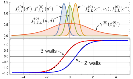
Figure 1: (bottom) The solid lines show the numerical solution for the diagonal elements of $T$ for $v=\sqrt{2}$, $\lambda=\Omega=1$, $\mu=0.81$ and $\alpha=1.1$. The broken curves stand for the analytic solution (15) for $V_{1}=0$ with the same separation $L=1$. (top) The mode functions of the fermions and massive gauge boson with $h=\tilde{h}=10$. The shared horizontal axis is $y$.

To figure out which is the true ground state configuration, we survey the parameter space $\alpha$-$\mu$ by using the gradient flow equation Manton:2004tk

$$\frac{\partial\phi(y,t^{\prime})}{\partial t^{\prime}}=-\frac{\delta S_{\rm E}}{\delta\phi(y,t^{\prime})}.$$ (31)

Here, $\phi$ stands for the scalar fields and we introduce a fictitious flow-time $t^{\prime}$ and let the field configuration relax toward the local minimum of the Euclidean action $S_{\rm E}$ as $t^{\prime}\to\infty$. To find global minima, we use initial configurations in (15) and solve the gradient flow equation with randomly chosen $Y$ for each point in the $\alpha$-$\mu$ space repeatedly. We confirm that there exists a large region in the $\alpha$-$\mu$ parameter space where the 3-2 splitting is the global minimum, see Fig. 2. Our resut shows that the attractive force given by the higher vacuum energy of the $\left<3,2\right>$ vacuum is balanced against an exponentially decaying repulsive force near domain walls.

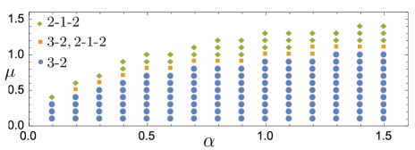
Figure 2: Minima in the $\alpha$-$\mu$ space. The 3-2 (2-1-2) splitting is the global minimum for the blue circle (green diamond). Both of them exist as global and local minima for the orange square ($v=\sqrt{2}$, $\lambda=\Omega=1$).

Taking all the parameters with mass dimension in $V_{0}$ and $V_{1}$ to be the same order of magnitude, and identify them with $M_{\rm GUT}$, the 3-2 walls are stabilized at the separation

$$L\sim M_{\rm GUT}^{-1},$$ (32)

as illustrated in Fig. 1. Thus, $V_{1}$ lifts the moduli in $t_{2,3}$ ($s_{2,3}$) and gives the mass

$$\tilde{\mu}_{0}\sim M_{\rm GUT}$$ (33)

to $b_{\mu}$. At the same time, we find that all the undesirable moduli fields are stabilized to have masses of order $M_{\rm GUT}$.

IV Quarks and Leptons

The Yukawa terms for $\Psi_{\bar{5},10}$ and $T$ provides massless chiral fermions around the domain walls. The fermion localization depends only on the solution $T$ which we can obtain reliably by numerically solving gradient flow even when $V_{1}\neq 0$. As shown in Fig. 1, difference between the numerical solution (solid curves) for $V_{1}\neq 0$ and the analytic solution (dashed curves) given in Eq. (15) is tiny. Thus, we can make use of (15) with $Y={\rm diag}({\cal Y}_{3},{\cal Y}_{3},{\cal Y}_{3},{\cal Y}_{2},{\cal Y}_{2})$ in the following. Let us decompose the fermions as $\bar{5}\to(\bar{3},1)_{1/3}\oplus(1,2)_{-1/2}$ and $10\to(\bar{3},1)_{-2/3}\oplus(3,2)_{1/6}\oplus(1,1)_{1}$

$$\Psi_{\bar{5}}=\left(\begin{matrix}\Psi_{\bar{3}}\\ \Psi_{2}\end{matrix}\right)\,,\quad\Psi_{10}=\left(\begin{matrix}\Psi_{\bar{3}}^{\prime}&\Psi_{3,2}\\ -\Psi_{3,2}^{t}&\Psi_{1}\end{matrix}\right)\,.$$ (34)

We expand fermions into modes such as

$$\Psi_{\bar{3}}=\sum_{n}\left[f_{\bar{3},L}^{(n)}(y)\psi_{\bar{3},L}^{(n)}(x)+f_{\bar{3},R}^{(n)}(y)\psi_{\bar{3},R}^{(n)}(x)\right],$$ (35)

where effective fields $\psi_{L,R}(x)$ are chiral fermions in $3+1$ dimensions defined by

$$\psi_{L}=P_{-}\psi,\quad\psi_{R}=P_{+}\psi,$$ (36)

with $P_{\pm}\equiv(1\pm\gamma^{5})/2$. Furthermore, four-dimensional gamma matrices $\gamma^{\mu}$ are defined from the five-dimensional gamma matrices $\Gamma^{M}$ as

$$\Gamma^{\mu}=\gamma^{\mu},\quad\Gamma^{5}=i\gamma^{5},\quad\gamma^{5}=i\gamma^{0}\gamma^{1}\gamma^{2}\gamma^{3}.$$ (37)

The other components can be expanded similarly. Plugging these into linearized field equations for $\Psi_{\bar{5},10}$, we find equations for mode functions

$${\cal H}_{X}f_{X}^{(n)}(y)=m_{X}^{(n)}{}^{2}f_{X}^{(n)}(y),$$ (38)

where the subscript $X$ distinguishes the components in Eq. (34). The Hamiltonian for the left component ${\cal H}_{X,L}$ and the right component ${\cal H}_{X,R}$ are

$${\cal H}_{X,L}=Q_{X}^{\dagger}Q_{X},\quad{\cal H}_{X,R}=Q_{X}Q_{X}^{\dagger},$$ (39)

with

$$Q_{X}=\partial_{y}+h_{X}(y),\quad Q_{X}^{\dagger}=-\partial_{y}+h_{X}(y).$$ (40)

The $y$-dependent effective Yukawa couplings are approximated by $h_{X}=h\tau_{3}$ for $\Psi_{\bar{3}}$, $\tilde{h}\tau_{3}$ for $\Psi_{\bar{3}}^{\prime}$, $h\tau_{2}$ for $\Psi_{2}$, $\tilde{h}\tau_{2}$ for $\Psi_{1}$, and $\tilde{h}(\tau_{3}+\tau_{2})/2$ for $\Psi_{3,2}$ using $\tau_{3}(y),\tau_{2}(y)$ defined in Eq.(26). The mode functions $f^{(0)}_{X}$ for zero modes are the kernels of $Q_{X}$ and $Q_{X}^{\dagger}$. When $h>0$ and $\tilde{h}>0$, the normalizable zero modes appear only in the left-handed components as

$$f_{\bar{3},L}^{(0)}=N_{\bar{3}}\left[\cosh\Omega(y-{\cal Y}_{3})\right]^{-\frac{hv}{\Omega}},$$ (41)

with the normalization constant $N_{\bar{3}}$. Similarly zero modes appear only for left-handed components $\psi_{\bar{3},L}^{\prime}$, $\psi_{2,L}$ and $\psi_{1,L}$, whose mode functions are obtained by replacing $h$ with $\tilde{h}$, and ${\cal Y}_{3}$ with ${\cal Y}_{2}$. The mode functions for $\psi_{3,2,L}$ are given as

$$\!\!\!\!\!\!\!\!\!\!\!\!\!\!f_{3,2,L}^{(0)}=N_{3,2}\left[\cosh\Omega(y-{\cal Y}_{3})\cosh\Omega(y-{\cal Y}_{2})\right]^{-\frac{\tilde{h}v}{2\Omega}}\,,$$ (42)

with the normalization constant $N_{3,2}$.

We identify one generation of quarks and leptons as usual

$$\psi_{\bar{3},L}^{(0)}\to d^{c}_{\alpha},\quad\psi_{\bar{3},L}^{(0)}{}^{\prime}\to u^{c}_{\alpha},\quad\psi_{2,L}^{(0)}\to l_{a}=(e^{-},\nu_{e}),$$ (43)

$$\psi_{1,L}^{(0)}\to e^{+},\quad\psi_{3,2,L}^{(0)}\to q_{\alpha a}=(u_{\alpha},\ d_{\alpha}).$$ (44)

We show typical mode functions in Fig. 1, where we observe that quarks and leptons are localized around the walls associated to the gauge fields with which they interact.

Maintaining charge universality has been difficult for localized gauge fields Rubakov2 ; Dubovsky:2001pe . In our model, the charge universality holds exactly since the $3+1$ dimensional SM gauge symmetry is fully maintained. In other words, the overlap integrals with the SM gauge fields and quarks (leptons) are independent of wall positions, since mode functions of massless gauge fields are flat $v_{\alpha}^{(0)}/\sigma_{\alpha}=1$ as in Eq.(23).

V Baryon number violating process

The massive gauge boson $\beta_{\mu}^{(0)}$ with mass $\tilde{\mu}_{0}\sim M_{\rm GUT}$ plays the same role as $X,Y$ gauge bosons in the usual $3+1$ dimensional GUT, where its exchange is suppressed by the large mass $M_{\rm GUT}$. When the symmetry breaking occurs by the wall splitting, however, their coupling to quarks and leptons can have significant additional suppression. This suppression results from the small overlap of mode functions caused by two factors: the quark and lepton mode functions can be displaced from each other ArkaniHamed:1999dc , and their mode functions are sharply peaked when their Yukawa couplings are large. The relevant triple couplings for the proton decay can be found in the kinetic terms of $\Psi_{\bar{5},10}$ as

$${\cal L}_{\rm PD} = gH_{{\rm lq1}}\bar{d}^{\rm c}\gamma^{\mu}\beta^{(0)*}_{\mu}l+gH_{\rm dq}\mathrm{Tr}_{3}\!\!\left[\bar{U}^{\rm c}\gamma^{\mu}\beta_{\mu}^{(0)}q^{t}\right]$$ (45)

$$+ ~{}gH_{{\rm lq2}}\mathrm{Tr}_{2}\!\!\left[\beta_{\mu}^{(0)t}\bar{q}\gamma^{\mu}E^{+}\right]+\text{h.c.}\,.$$

Here, we use the canonical normalization for the massive gauge bosons by redefining $\beta_{\mu}^{(0)}\to g\beta_{\mu}^{(0)}$, and identify fermion zero modes as

$$(E^{+})_{ab}=\epsilon_{ab}e^{+},\quad(U^{\rm c})_{ab}=\epsilon_{abc}u^{\rm c}_{c}.$$ (46)

The triple couplings depend on the separation $L$ between the domain walls and are given by the overlap integrals

$$H_{Z}(L)=\int_{-\infty}^{\infty}dy\,r_{Z},$$ (47)

for the channel $Z={\rm lq1},\,{\rm lq2},\,{\rm dq}$ with the integrand given by

$$r_{{\rm lq1}}=\frac{f_{\bar{3},L}^{(0)}f_{2,L}^{(0)}\gamma^{(0)}}{\sigma_{+}},$$ (48)

$$r_{{\rm lq2}}=\frac{2f_{1,L}^{(0)}f_{3,2,L}^{(0)}\gamma^{(0)}}{\sigma_{+}},$$ (49)

$$r_{\rm dq}=\frac{2f_{\bar{3},L}^{\prime(0)}f_{3,2,L}^{(0)}\gamma^{(0)}}{\sigma_{+}}.$$ (50)

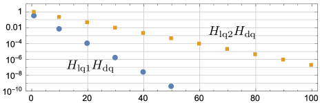
Figure 3: Suppression factor $H_{\rm lq1}H_{\rm dq}$ (blue circle) and $H_{\rm lq2}H_{\rm dq}$ (orange square) as a function of $h=\tilde{h}$. The parameters are $v=\sqrt{2}$ and $\Omega=\lambda=1$ and we set $L=1$.

The effective four-fermi coupling ${\cal G}_{ZZ^{\prime}}$ for the process $Z\to Z^{\prime}$ is given by

$${\cal G}_{ZZ^{\prime}}=\frac{H_{Z}H_{Z^{\prime}}g^{2}}{\tilde{\mu}_{0}^{2}}\,.$$ (51)

The suppression factors $H_{Z}$, and $H_{Z^{\prime}}$ compared to the standard GUT is calculable in our model, since the mode function $\gamma^{(0)}(y)$, shown in Fig. 1, is reliably obtained unlike in the previous model Dvali:1996xe based on an ambitious assumption of nonperturbative confinement in $4+1$ dimensions. On top of being a function of separation $L$ between walls, $H_{Z,Z^{\prime}}$ also depends strongly on the magnitude of Yukawa couplings $h$ and $\tilde{h}$. The width of the mode function is inversely proportional to Yukawa couplings $h$ and $\tilde{h}$. Hence the large Yukwa coupling suppresses the overlap exponentially $H_{Z}\sim e^{-vhL}$. We plot $H_{\rm lq1}H_{\rm dq}$ and $H_{\rm lq2}H_{\rm dq}$ in Fig. 3, where we see that they are suppressed by more than $10^{-3}$ and $10^{-9}$, respectively, with the Yukawa coupling of order $50$. We note that there is no constraints from experimental data for these large Yukawa couplings between fermions and scalars forming the domain wall.

Finally let us consider the baryon number violating process mediated by the off-diagonal component $\tilde{t}$ of scalar field $T$ through the Yukawa couplings. Although it is difficult to solve the Schrödinger problem for $\tilde{t}$ 1stpaper analytically, it is still possible to get qualitative features. Since the zero modes of $\tilde{t}$ are absorbed by $b_{\mu}$, the lightest mode of $\tilde{t}$ should have mass of order $M_{\rm GUT}$. In addition, since the potential of the Schrödinger problem should make the mode functions localized around the walls, similarly to zero mode case, the overlaps of mode functions are suppressed similarly to the vector case. Hence we expect that $T$-mediated proton decay enjoys a suppression factor of the same order as that of the massive vector bosons.

VI Conclusion

We propose a $4+1$ dimensional model which unifies $SU(5)$ GUT and the brane world scenario. Our $3+1$ dimensional spacetime dynamically emerges with the symmetry breaking $SU(5)\to G_{\rm SM}$ together with one generation of the SM matter fields. We solve the gradient flow equation and confirm the 3-2 splitting configuration is the global minimum in a large parameter region. By applying the idea of the field-dependent gauge kinetic function Ohta ; Us1 ; Us2 to our model, we solve the long-standing difficulties of the localization of massless gauge fields and charge universality. All the undesirable moduli are stabilized. Furthermore, the proton decay can be exponentially suppressed.

Our model is an effective theory valid up to the GUT energy scale which is characterized by the inverse of the width of the domain wall. Above this GUT scale, we need to take account of effects of strong gauge dynamics, since our gauge field localization mechnism is based on a semi-classical representation of confinement in the bulk away from domain walls. Below the GUT scale, the SM gauge couplings run following the usual renormalization group flow dictated by the low-energy effective Lagrangian in four dimensions. However, above the GUT scale, the effects of strong gauge dynamics should contribute to the running and change its behavior, in addition to the fact that the theory becomes five-dimensional. The quantum theory of our model above the GUT scale is an interesting subtle issue to study as a future work.

We have not yet included the SM Higgs field Maru:2001ch ; Haba:2002if and the second and higher generations, but our framework can easily incorporate the former similarly to Ref. Volkas and the latter with the mass hierarchy in the spirit of Ref. ArkaniHamed:1999dc ; Dvali2 . Furthermore, our model can be extended to other GUT gauge groups such as $SO(10)$. Supersymmetry and/or warped spacetime with gravity can also be included without serious difficulties. Since our model has strong resemblance to D-branes in superstring theory, we hope that our field theoretical model can give some hints for simple constructions of SM by D-branes.

- (1) J. C. Pati and A. Salam, Phys. Rev. D 8 (1973) 1240.
- (2) H. Georgi and S. L. Glashow, Phys. Rev. Lett. 32 (1974) 438.
- (3) H. Georgi, H. R. Quinn and S. Weinberg, Phys. Rev. Lett. 33 (1974) 451.
- (4) E. Witten, Nucl. Phys. B 188 (1981) 513.
- (5) S. Dimopoulos and H. Georgi, Nucl. Phys. B 193 (1981) 150.
- (6) N. Sakai, Z. Phys. C 11 (1981) 153.
- (7) S. Dimopoulos, S. Raby and F. Wilczek, Phys. Rev. D 24 (1981) 1681.
- (8) N. Arkani-Hamed, S. Dimopoulos and G. R. Dvali, Phys. Lett. B 429, 263 (1998) [hep-ph/9803315].
- (9) I. Antoniadis, N. Arkani-Hamed, S. Dimopoulos and G. R. Dvali, Phys. Lett. B 436, 257 (1998). [hep-ph/9804398].
- (10) L. Randall and R. Sundrum, Phys. Rev. Lett. 83 (1999) 3370. [hep-ph/9905221].
- (11) L. Randall and R. Sundrum, Phys. Rev. Lett. 83 (1999) 4690. [hep-th/9906064].
- (12) K. Akama, Lect. Notes Phys. 176 (1982) 267. [hep-th/0001113].
- (13) Y. Kawamura, Prog. Theor. Phys. 103 (2000) 613 [hep-ph/9902423].
- (14) Y. Kawamura, Prog. Theor. Phys. 105 (2001) 999 [hep-ph/0012125].
- (15) Y. Kawamura, Prog. Theor. Phys. 105 (2001) 691 [hep-ph/0012352].
- (16) G. Altarelli and F. Feruglio, Phys. Lett. B 511 (2001) 257 [hep-ph/0102301].
- (17) L. J. Hall and Y. Nomura, Phys. Rev. D 64 (2001) 055003 [hep-ph/0103125].
- (18) A. Hebecker and J. March-Russell, Nucl. Phys. B 613 (2001) 3 [hep-ph/0106166].
- (19) V. A. Rubakov and M. E. Shaposhnikov, Phys. Lett. 125B (1983) 136.
- (20) R. Davies, D. P. George and R. R. Volkas, Phys. Rev. D 77 (2008) 124038.
- (21) A. Davidson, D. P. George, A. Kobakhidze, R. R. Volkas and K. C. Wali, Phys. Rev. D 77 (2008) 085031.
- (22) J. E. Thompson and R. R. Volkas, Phys. Rev. D 80 (2009) 125016.
- (23) B. D. Callen and R. R. Volkas, Phys. Rev. D 83 (2011) 056004.
- (24) B. D. Callen and R. R. Volkas, Phys. Rev. D 86 (2012) 056007.
- (25) G. R. Dvali and M. A. Shifman, Phys. Lett. B 396 (1997) 64 [Erratum-ibid. B 407 (1997) 452].
- (26) G. R. Dvali, G. Gabadadze and M. A. Shifman, Phys. Lett. B 497 (2001) 271.
- (27) A. Kehagias and K. Tamvakis, Phys. Lett. B 504 (2001) 38.
- (28) S. L. Dubovsky and V. A. Rubakov, Int. J. Mod. Phys. A 16 (2001) 4331.
- (29) K. Ghoroku and A. Nakamura, Phys. Rev. D 65 (2002) 084017.
- (30) E. K. Akhmedov, Phys. Lett. B 521 (2001) 79.
- (31) I. I. Kogan, S. Mouslopoulos, A. Papazoglou and G. G. Ross, Nucl. Phys. B 615 (2001) 191.
- (32) H. Abe, T. Kobayashi, N. Maru and K. Yoshioka, Phys. Rev. D 67 (2003) 045019.
- (33) M. Laine, H. B. Meyer, K. Rummukainen and M. Shaposhnikov, JHEP 0301 (2003) 068.
- (34) N. Maru and N. Sakai, Prog. Theor. Phys. 111 (2004) 907.
- (35) B. Batell and T. Gherghetta, Phys. Rev. D 75 (2007) 025022.
- (36) R. Guerrero, A. Melfo, N. Pantoja and R. O. Rodriguez, Phys. Rev. D 81 (2010) 086004.
- (37) W. T. Cruz, M. O. Tahim and C. A. S. Almeida, Phys. Lett. B 686 (2010) 259.
- (38) A. E. R. Chumbes, J. M. Hoff da Silva and M. B. Hott, Phys. Rev. D 85 (2012) 085003.
- (39) C. Germani, Phys. Rev. D 85 (2012) 055025 [arXiv:1109.3718 [hep-ph]].
- (40) T. Delsate and N. Sawado, Phys. Rev. D 85 (2012) 065025.
- (41) W. T. Cruz, A. R. P. Lima and C. A. S. Almeida, Phys. Rev. D 87 (2013) no.4, 045018.
- (42) A. Herrera-Aguilar, A. D. Rojas and E. Santos-Rodriguez, Eur. Phys. J. C 74 (2014) no.4, 2770.
- (43) Z. H. Zhao, Y. X. Liu and Y. Zhong, Phys. Rev. D 90 (2014) no.4, 045031.
- (44) C. A. Vaquera-Araujo and O. Corradini, Eur. Phys. J. C 75 (2015) no.2, 48.
- (45) J. B. Kogut and L. Susskind, Phys. Rev. D 9 (1974) 3501.
- (46) R. Fukuda, Phys. Lett. B 73 (1978) 305 [Erratum-ibid. B 74 (1978) 433];Mod. Phys. Lett. A 24 (2009) 251;arXiv:0805.3864 [hep-th].
- (47) K. Ohta and N. Sakai, Prog. Theor. Phys. 124 (2010) 71 Erratum: [Prog. Theor. Phys. 127 (2012) 1133].
- (48) M. Arai, F. Blaschke, M. Eto and N. Sakai, PTEP 2013 (2013) 013B05.
- (49) M. Arai, F. Blaschke, M. Eto and N. Sakai, PTEP 2013 (2013) no.9, 093B01.
- (50) M. Arai, F. Blaschke, M. Eto and N. Sakai, PTEP 2017 (2017) no.5, 053B01.
- (51) V. A. Rubakov, Phys. Usp. 44 (2001) 871 [Usp. Fiz. Nauk 171 (2001) 913].
- (52) N. S. Manton and P. Sutcliffe, “Topological solitons,” Cambridge University Press, 2007.
- (53) N. Maru, Phys. Lett. B 522, 117 (2001).
- (54) N. Haba and N. Maru, Phys. Lett. B 532, 93 (2002).
- (55) N. Arkani-Hamed and M. Schmaltz, Phys. Rev. D 61 (2000) 033005.
- (56) G. R. Dvali and M. A. Shifman, Phys. Lett. B 475 (2000) 295.