Voids in the Cosmic Web as a probe of dark energy

Abstract

The formation of large voids in the Cosmic Web from the initial adiabatic cosmological perturbations of space-time metric, density and velocity of matter is investigated in cosmological model with the dynamical dark energy accelerating expansion of the Universe. It is shown that the negative density perturbations with the initial radius of about 50 Mpc in comoving to the cosmological background coordinates and the amplitude corresponding to the r.m.s. temperature fluctuations of the cosmic microwave background lead to the formation of voids with the density contrast up to $-$0.9, maximal peculiar velocity about 400 km/s and the radius close to the initial one. An important feature of voids formation from the analyzed initial amplitudes and profiles is establishing the surrounding overdensity shell. We have shown that the ratio of the peculiar velocity in units of the Hubble flow to the density contrast in the central part of a void does not depend or weakly depends on the distance from the center of the void. It is also shown that this ratio is sensitive to the values of dark energy parameters and can be used to find them based on the observational data on mass density and peculiar velocities of galaxies in the voids.

Key words: cosmological perturbations, dark energy, large scale structure of the Universe, voids, Cosmic Web

PACS: 95.36.+x, 98.80.-k

Abstract

В роботi дослiджено формування великих порожнин з початкових космологiчних адiабатичних збурень метрики простору-часу та густини i швидкостi матерiї в моделях Всесвiту з динамiчною темною енергiєю, що зумовлює прискорене розширення Всесвiту. Показано, що вiд’ємнi збурення густини з початковим розмiром близько 50 Mpc в супутнiх до космологiчного фону координатах та амплiтудою, що вiдповiдає спостережуваним середньоквадратичним флуктуацiям температури мiкрохвильового релiктового випромiнювання, приводять до утворення порожнин з контрастом густини матерiї аж до $-$0.9, максимумом пекулярної швидкостi близько 400 км/c та з радiусом близьким до початкового. Важливою особливiстю дослiджених початкових профiлiв густини є формування оточуючої оболонки згущення. Показано, що вiдношення пекулярної швидкостi в одиницях габблiвського потоку до контрасту густини в центральнiй частинi порожнини не залежить або слабо залежить вiд вiдстанi вiд центра порожнини. Показано, що таке спiввiдношення є чутливим до значень параметрiв темної енергiї i може бути використане для їх знаходження на основi даних про структуру порожнин та пекулярнi швидкостi галактик у них.

Ключовi слова: космологiчнi збурення, темна енергiя, великомасштабна структура Всесвiту, порожнини, космiчна павутина

1 Introduction

The cosmological constant, which has been introduced into general relativity one hundred years ago by Albert Einstein [1], played an important role in the development of the theory of structure and evolution of the Universe. Late in the 20th century, two research teams, SuperNova Cosmology Project and High-z SuperNova Search, performed the cosmological test ‘‘magnitude–redshift’’ for type Ia supernovae and obtained secure observational evidence (at 3$\sigma$ confidence level) for non-zero positive value of the cosmological constant [2, 3, 4] and accelerated expansion of the Universe as a consequence. Since the cosmological constant has no consistent physical interpretation, other essences have been proposed to explain the accelerated expansion of the Universe. They have been commonly referred to as the ‘‘dark energy’’ [5]. Among them the most elaborated ones are the scalar field models of dark energy [6, 7, 8, 9]. In the ‘‘world ocean’’ of different variants of such models one can distinguish a few ‘‘main streams’’, such as quintessential, phantom, quintom and others. Accurate observations and new crucial tests are needed to discriminate between these candidates and decide which one fills our Universe. In numerous papers of the last decade it was shown that large voids in a large-scale structure of the Universe are excellent laboratories for this purpose [10, 11, 12, 13, 14, 15, 16, 17, 18, 19, 20]. Here, we show that the data on dynamical structure of the voids, positions, number densities and peculiar velocities of the galaxies at central parts of the voids are sensitive to the parameters of dark energy.

2 Voids in Cosmic Web

The space distribution of luminous matter, which is collected in galaxies, forms a large-scale structure of the Universe. Its elements — clusters, superclusters, walls, sheets, filaments, nodes and voids — form a complex geometrical and topological system which is sometimes dubbed as the Cosmic Web [21]. It emerged from the quantum fluctuations of space-time metric generated in the early universe and stretched to the cosmic scale by inflation. Its formation in the expanding Universe is a long history of action of the forces of self-gravitation of luminous matter, gravity of dark matter and ‘‘anti-gravity’’ of dark energy on large scales. The complexity of the structure requires sophisticated methods of analysis. Methods of complex systems analysis which have been recently developed [22, 23, 24] may be helpful in understanding the hidden patterns of such structures. In this section we will walk through the history of the study of voids and shortly review the most prominent recent works in this field.

In 1978 Gregory and Thompson [25] and independently of them Joeveer, Einasto and Tago [26], while studying superclusters, noticed that there are areas in the galaxy field where the galaxy density is much lower than the average one (Joeveer referred to them as the ‘‘holes’’ in the distribution). Very soon it became obvious that these holes — or, as we call them now, cosmic voids — are very important in the matter distribution and its evolution. In the 1980s there appeared papers by renowned cosmologists (Zeldovich [27] and Silk [28]) devoted to the cosmic voids. They showed that primordial adiabatic cosmological perturbations were the progenitors of voids, the same as for the clusters and galaxies, but with the opposite sign. In the same period, first papers analytically describing the evolution of voids with a certain profile were written by Sato [29] and Maeda [30]. The analytic solutions of the evolution equations for voids predicted already some important features of the voids, in particular, their expansion during evolution, in contrast to the collapse of halos, and the formation of an overdensity shell, the same as we observe in our numerical solutions. Another important feature, i.e., tendency to sphericity of the voids, was shown by Fujimoto [31] and Icke [32].

Unlike the clusters and galaxies, cosmic voids are much harder to track, because they are underdense and hence unluminous. So, it is not surprising that the $N$-body cosmological simulation of the large-scale distribution became a powerful tool in studying the voids, since they have an observational fullness of the void population in comparison with the real distribution. The first papers describing the voids in a numerical simulation were written in 1984 [33].

Quite soon, the amount of data on large-scale structure of the Universe increased quite enough, so that the properties of cosmic voids began being studied statistically. Already in 1985, Vettolani and colleagues gave statistics on the volume distribution of 200 real voids [34]. The latest and the largest galaxy catalogue, on which the void-finding algorithm was imposed, is SDSS DR12. Mao and colleagues have found more than 10 000 voids there in the redshift range $0.1<z<0.7$ [35].

In the late 1980s the papers discussing the lack of voids in the Ly-alpha forest began to emerge [36, 37]. Due to the faintness of young galaxies, the discovery of voids at $z>1$ was made only in 1991 [38]. The modern searches for early voids in cosmological simulations were carried out in [39] and in observable data in [40], highlighting, probably, the most distant observable voids at $z=5.7$ in the spatial distributions of the Lyman-alpha emitters.

Nevertheless, many secrets of the voids’ nature were discovered in distributions obtained from numerical simulations, including the void universal density profile [41]. The $\Lambda$CDM cosmology simulation with probably the largest number of voids was done in 2004, where in total 80 000 voids were found in the simulated distribution [42]. Another interesting work was written by Gottlober and colleagues [43], where they studied the mass distribution in voids, halos in them, the void mass function and its dependence on the radius using the results of high-resolution $N$-body simulations. With the development of such simulations, it became possible to track the evolution of voids in such simulated universes. The authors of [44, 45, 46] studied the changes of profiles and sizes of the void population with $z$. Modern results on voids from $N$-body simulations are given in [46, 47].

The influence of surroundings on the formation of voids as well as their hierarchical structure became clear in 1990s and in early 2000s. Being underdense fragile structures, the voids can be crushed by the infall of outer regions (i.e., void collapse) or merge into a larger void. The first paper describing the void clustering was written in 1994 by Haque-Copilah and Basu [48], the interaction of two voids was considered in 1993 by Dubinski [49]. In 2003–2004 van de Weygaert and Sheth wrote several papers [50, 51], summing up the studies of the void hierarchy problem. In the latter paper, the authors managed to formulate the excursion set formalism of void formation and evolution in the manner like it was previously done for halos (see also [14] and [15]). They give clear classification of the types of voids and their density depending on their neighborhood (void-in-clouds and void-in-voids). They also sum up the general properties of voids studied at that time.

Starting from the paper [52], the void statistics is used for constraining different cosmological parameters [17], probing the dark energy [11, 12, 18], testing the modified gravity [13, 10, 14, 16]. After Amendola and colleagues computed the weak gravitational lensing by voids [53] it became possible to find the constraints on cosmological parameters from the influence of this lensing on the cosmic microwave background (CMB) [54] (an example of how voids can be studied through the gravitational lensing produced by them is given in [55]). Another important cosmological test, the Alcock-Paczynski test [56], was predicted and tested in the $N$-body simulation by Lavaux [57] and then confirmed by the observational data by Sutter and team [58]. They used the stacked cosmic voids identified in the SDSS DR7 and DR10 and measured their ellipticity. The essence of this test is in the statistical study of the form of large-scale structures. If one uses a correct cosmology, the relation of sizes along and transverse the line of sight shows no dependence on $z$. The results confirmed that the dark energy has no alternatives, but they do not distinguish between the models of dark energy.

In 2008, Neyrinck published [59] the algorithm for finding the voids in 3D-galaxy distribution called Zones Bordering On Voidness (ZOBOV). This algorithm uses the Voronoi tessellation to divide the volume into regions with some averaged density. The center of each Voronoi cell is one galaxy. After that, it applies the watershed landform to the obtained 3D density map to find the edges of voids. ZOBOV algorithm is claimed to be free of parameters and assumptions about the shapes of expected voids. It became really popular among the researchers and they now usually use ZOBOV or its modifications (like, for example, project VIDE [60]) to find voids in the cosmological simulation data or real galaxy catalogs.

Despite the far from spherical shape of the walls of the most voids and the influence of surroundings, the study of the evolution of a spherical isolated void supplies us with valuable hints in describing the main physical characteristics of the void, sometimes including astonishingly accurate quantitative guidelines [47]. The universal density profile of a spherical void has been proposed by Hamaus, Sutter and Wandelt [41]. The profile has 4 parameters characterizing the size and steepness of the void and its overdensity shell. The authors argue that there is some relation between the form of a void and its size and hence the parameters are not independent. They show possible dependences that may exist. This work causes a wide discussion. For example, experts are disputing whether the parameters of stacked voids profile would be the same [61] or different [62] for the simulation and real galaxy distribution.

Finally, we would like to emphasise the role of voids as a probe of dark energy. Li [63] has shown that voids can be used to rule out observationally or distinguish between coupled scalar field models of dark energy. Voids are also sensitive to the massive gravity dark energy models [64]. Usually, the shape of voids is studied statistically to constrain the parameters of dark energy [11, 12, 65]. Moreover, with universal density profile, one can improve the Alcock-Paczynski test by specifying the galaxies’ redshift distortion and recovering the shape of voids, which, again, help to constrain the dark energy parameters [17, 18]. Our work is an essential complement to these ones, allowing to follow the evolution of a single void with all its features.

3 Spherical voids: the dependence of velocity to density perturbations ratio on dark energy parameters

In our previous papers [19, 20] we analysed the formation of single spherical voids in the three-component medium (matter, radiation and dark energy) from the early epoch up to the current one. We described each component in the hydrodynamical approximation. The model of minimally coupled dynamical dark energy had three free parameters: the energy density in units of the critical one at current epoch $\Omega_{\text{de}}\equiv 8\pi G\varepsilon^{0}_{\text{de}}/3H_{0}^{2}$, the equation of state parameter $w_{\text{de}}\equiv p_{\text{de}}/\varepsilon_{\text{de}}$ and the squared effective sound speed $c_{\text{s}}^{2}\equiv\delta p_{\text{de}}/\delta\varepsilon_{\text{de}}$ in the rest frame of dark energy. We assumed that the last two parameters are constant. Here and below we use the units in which the speed of light in vacuum $c=1$, all velocities are in the units of speed of light.

We have shown in [20] how the spherical cosmological perturbation evolves to form the void with approximately universal density and velocity profiles. Here, we will show that the ratio of matter velocity and density perturbations, which can in principle be measured, is sensitive to the values of main parameters of the dynamical dark energy. This ratio does not depend on the initial amplitude at the linear stage of evolution. Since large voids in the spatial distribution of matter, traced by galaxies, are now at quasi-linear stage of their evolution, the dependence on the initial amplitude is predictable and can be estimated from the numerical calculations or $N$-body simulations. On the other hand, large voids in the Cosmic Web are almost spherical, so the dependence of this ratio on the profile of initial perturbation and the impact of environment can be also removed, at least for the central part of voids. In this work we only outline the key dependences for the new possible test and leave the mentioned here important aspects of its implementation for future papers.

3.1 Assumptions and equations

Let us consider the evolution of spherical adiabatic cosmological perturbations in the Universe filled with the matter, dynamical dark energy and relativistic component. The last one is important in the early Universe when we set the initial conditions following from the observational data on the CMB anisotropy (see for details [20]). We present the space-time metric in the region of a perturbation in the Newtonian gauge as follows:

$$\mathrm{d}s^{2}=\mathrm{e}^{\nu(t,r)}\mathrm{d}t^{2}-a^{2}(t)\mathrm{e}^{-\nu(t,r)}\left[\mathrm{d}r^{2}+r^{2}(\mathrm{d}\theta^{2}+\sin^{2}\theta\mathrm{d}\varphi^{2})\right],$$ (3.1)

where $t$ is the cosmological time, $r$ is the radial coordinate comoving to the unperturbed background, $\theta$ and $\varphi$ are the polar and azimuth angles in the spherical 3D coordinates and $a(t)$ is the scale factor of cosmological background. The function $\nu(t,r)$ is the metric perturbation caused by the local density perturbation of all components. At distances larger than the radius of void, $r\gg r_{\text{v}}$, $\nu(t,r)\rightarrow 0$ and the metric (3.1) becomes the Friedmann-Lemaitre-Robertson-Walker (FLRW) one. The time dependence of the scale factor is determined by the Friedmann equation

$$H^{2}\equiv\left(\frac{\mathrm{d}\ln{a}}{\mathrm{d}t}\right)^{2}=H_{0}^{2}\left[\Omega_{\text{rel}}a^{-4}+\Omega_{\text{m}}a^{-3}+\Omega_{\text{k}}a^{-2}+\Omega_{\text{de}}a^{-3(1+w_{\text{de}})}\right].$$ (3.2)

In the computations below we set the Hubble constant $H_{0}$ to be 70 $\text{km}/{\text{s}}\cdot\text{Mpc}$, this value lies between the ‘‘global’’ ($67.8\pm 0.9$ $\text{km}/{\text{s}}\cdot\text{Mpc}$ [66]) and ‘‘local’’ ($73.24\pm 0.74$ $\text{km}/{\text{s}}\cdot\text{Mpc}$ [67]) measurements. The spatial curvature, as the Planck 2015 results show, is very close to zero with $|\Omega_{\text{k}}|<0.005$, that is why in the most of computations we will put it equal to zero.

In the spherical perturbed region, the contravariant components of 4-velocity of any component $u^{i}_{N}\equiv\mathrm{d}x^{i}/\mathrm{d}s$ in the metric (3.1) are

$$u^{i}_{N}(t,r)=\left\{\frac{\mathrm{e}^{-\nu/2}}{\sqrt{1-v_{N}^{2}}}\,,\,\,\frac{\mathrm{e}^{\nu/2}v_{N}}{a\sqrt{1-v_{N}^{2}}}\,,\,\,0,\,\,0\right\},$$ (3.3)

where the radial component of 3-velocity $v_{N}$ is defined as the ratio of proper space interval to proper time interval at the distance $r$ from the center of the void: $v_{N}(t,r)=\mathrm{e}^{-\nu}\mathrm{d}r/\mathrm{d}t$ (in units of speed of light). In the $v_{N}\ll 1$ approximation, the components of energy-momentum tensor of any component $T^{i}_{j\,(N)}=(\varepsilon_{N}+p_{N})u^{i}_{N}(t,r)u_{j\,(N)}-\delta^{i}_{j}p_{N}$ to the second order of smallness are as follows:

$$T^{0}_{0\,(N)} =\varepsilon_{N}+(\varepsilon_{N}+p_{N})v_{N}^{2}\,,\qquad T^{1}_{0\,(N)}=(\varepsilon_{N}+p_{N})\frac{\mathrm{e}^{\nu}}{a}v_{N}\,,$$ (3.4)

$$T^{1}_{1\,(N)} =-p_{N}-(\varepsilon_{N}+p_{N})v_{N}^{2}\,,\qquad T^{2}_{2\,(N)}=T^{3}_{3\,(N)}=p_{N}\,.$$ (3.5)

We present the energy density of every component as a sum of the mean (or background) value $\bar{\varepsilon}_{N}(t)$ and the local perturbation: $\varepsilon_{N}(t,r)=\bar{\varepsilon}_{N}(t)[1+\delta_{N}(t,r)]$, where $\delta_{N}$ denotes the relative density perturbation. The pressure of every component in the void is presented as $p_{N}(t,r)=w_{N}\bar{\varepsilon}_{N}(t)+\delta p_{N}(t,r)$. For the scalar field models of dark energy, the non-adiabatic component of pressure perturbation $\delta p_{N}(t,r)$ is important (see appendix A in [68] and references therein). Taking this into account, the pressure perturbation of any component in the generalised form can be presented as

$$\delta p_{N}(t,r)=c^{2}_{\text{s}\,(N)}\bar{\varepsilon}_{N}\delta_{N}(t,r)-3\bar{\varepsilon}_{N}aH(1+w_{N})\big{[}c^{2}_{\text{s}\,(N)}-w_{N}\big{]}\int{v_{N}(t,r)\mathrm{d}r}.$$

For the relativistic component with $c^{2}_{\text{s}\,(\text{rel})}=w_{\text{rel}}=1/3$ and the matter one with $c^{2}_{\text{s}\,(\text{m})}=w_{\text{m}}=0$, the non-adiabatic term disappears.

Therefore, in the metric (3.1) the Einstein equation $G^{0}_{0}=\varkappa T^{0}_{0}$ and the conservation law $T^{j}_{i\,;j}=0$ give us the system of equations for metric, density and velocity perturbations of the matter, dark energy and relativistic components in the expanding Universe with dynamical dark energy:

$$\nu^{\prime\prime} +\frac{2}{r}\nu^{\prime}-3a^{2}H^{2}(a\dot{\nu}+\nu)=3H^{2}_{0}\left[\Omega_{\text{m}}a^{-1}\delta_{\text{m}}+\Omega_{\text{rel}}a^{-2}\delta_{\text{rel}}+\Omega_{\text{de}}a^{-(1+3w)}\delta_{\text{de}}\right],$$ (3.6)

$$\dot{\delta}_{N} +\frac{3}{a}\left(c_{\text{s}}^{2}-w_{N}\right)\delta_{N}+(1+w_{N})\left[\frac{v^{\prime}_{N}}{a^{2}H}+\frac{2v_{N}}{a^{2}Hr}-9H\left(c_{\text{s}}^{2}-w_{N}\right)\int{v_{N}\mathrm{d}r}-\frac{3}{2}\dot{\nu}\right]$$

$$+\left(1+c_{\text{s}}^{2}\right)\left[\frac{\delta^{\prime}_{N}v_{N}}{a^{2}H}+\frac{\delta_{N}}{a^{2}H}\left(v^{\prime}_{N}+\frac{2}{r}v_{N}\right)-\frac{3}{2}\delta_{N}\dot{\nu}\right]=0,$$ (3.7)

$$\dot{v}_{N} +\left(1-3c_{\text{s}}^{2}\right)\frac{v_{N}}{a}+\frac{c_{\text{s}}^{2}\delta^{\prime}_{N}}{a^{2}H(1+w_{N})}+\left(1+\frac{1+c_{\text{s}}^{2}}{1+w_{N}}\delta_{N}\right)\frac{2v_{N}}{a^{2}H}\left(v_{N}^{\prime}+\frac{v_{N}}{r}\right)+\frac{\nu^{\prime}}{2a^{2}H}$$

$$+\frac{1+c_{\text{s}}^{2}}{1+w_{N}}\left[\dot{\delta}_{N}v_{N}+\delta_{N}\dot{v}_{N}+(1-3w_{N})\frac{\delta_{N}}{a}v_{N}+\frac{\nu^{\prime}\delta_{N}}{2a^{2}H}\right]=0.$$ (3.8)

We have rewritten the derivatives with respect to the time $\frac{\mathrm{d}}{\mathrm{d}t}$ as the derivatives with respect to the scale factor $\frac{\mathrm{d}}{\mathrm{d}t}=aH\frac{\mathrm{d}}{\mathrm{d}a}$ and denoted them as $(\,\,\dot{}\,\,)$. The derivatives with respect to the radial coordinate $\frac{\mathrm{d}}{\mathrm{d}r}$ are denoted here as $(\,^{\prime}\,)$. So, the system (3.6)–(3.8) for 7 unknown functions must be integrated with respect to the scale factor $a$ together with the algebraic equation (3.2). To integrate them, the initial conditions must be set.

3.2 Initial conditions

We set the initial conditions in the early epoch when the amplitudes of perturbations are small [$\delta_{N}(a,r)\ll 1$, $v_{N}(a,r)\ll 1$ and $\nu(a,r)\ll 1$] and the scale of perturbation is essentially larger than the particle horizon. For the radiation dominated epoch, we obtain, from the superhorizon asymptotic for the growth mode of cosmological perturbations, the relations between initial amplitudes:

$$\frac{4}{3}\delta_{\text{m}}(a_{\text{init}},r)=\frac{4}{3}\frac{\delta_{\text{de}}(a_{\text{init}},r)}{1+w_{\text{de}}}=\delta_{\text{rel}}(a_{\text{init}},r)=-\nu(a_{\text{init}},r),$$ (3.9)

$$v_{\text{m}}(a_{\text{init}},r)=v_{\text{de}}(a_{\text{init}},r)=v_{\text{rel}}(a_{\text{init}},r)=-\frac{\nu^{\prime}(a_{\text{init}},r)}{4a_{\text{init}}H(a_{\text{init}})}\,.$$ (3.10)

We set the local initial perturbation as a bell-like hill for the metric function $\nu(a_{\text{init}},r)=C(1-\kappa^{2}r^{2})\linebreak\times\exp(-r^{2}/r_{\text{d}}^{2})$ and an inverted bell-like profile for the density, where a free constant $C$ may be linked to the amplitude of the power spectrum of curvature perturbations measured at the last scattering surface of relic thermal radiation (see for details [20, 68]). We put here $C=3\cdot 10^{-4}$. We specify other parameters of this profile, which define the initial size and the slope of wall, as follows: $\kappa^{-1}=50~{}\text{Mpc}$, $r_{\text{d}}=25~{}\text{Mpc}.$

The initial profiles of matter density perturbations $\delta_{\text{m}}(a_{\text{init}},r)$, $\delta_{\text{de}}(a_{\text{init}},r)$, velocity $v_{\text{m}}(a_{\text{init}},r)\linebreak=v_{\text{de}}(a_{\text{init}},r)=v_{\text{rel}}(a_{\text{init}},r)$ and gravitational potential $\nu(a_{\text{init}},r)$ are presented in the left-hand panel of figure 1.

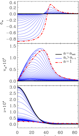
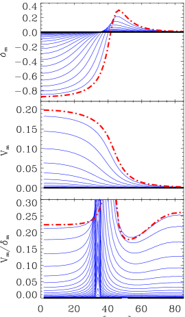
Figure 1: (Color online) Formation of the void from the cosmological spherical perturbation. Left-hand column: the initial profiles of density and velocity perturbations of matter and gravitational potential. Central column: evolution of the density $\delta_{\text{m}}$ and velocity $v_{\text{m}}$ perturbations of matter and gravitational potential $\nu$ from the initial profiles (thick black lines) to the final one at $a=1$ (thick dashed red lines). Right-hand column: evolution of the density perturbation (top), the velocity in units of the Hubble flow $V_{\text{m}}$ (middle) and the ratio $V_{\text{m}}/|\delta_{\text{m}}|$ (bottom).

3.3 Results and discussions

For numerical integration of the system of equations (3.6)–(3.8) with initial conditions (3.9)–(3.10), we have used the code npdes.f. The results are presented in the central panel of figure 1. It illustrates how the initial spherical matter density perturbation in the form of an inverted bell-like underdense profile with initial amplitude $\delta_{\text{m}}(a_{\text{init}},r=0)=-2.25\cdot 10^{-4}$ and radius $r_{\text{v}}\equiv\kappa^{-1}=50$ Mpc evolves to the spherical void with density contrast $\delta_{\text{m}}(a=1,r=0)\approx-0.9$ and comoving radius $r_{\delta=0}\approx 42$ Mpc. The matter, which is flowing from the central part of the void outwards, is collected in its peripheral part, forming an overdense shell and reducing somewhat the size of the void in the comoving coordinates.

Maximum of the peculiar velocity of matter is reached at 6/7 of the void final radius and is $v_{\text{m}}(1,r_{\text{max\,v}})\linebreak\approx 400$ km/s. The value of Hubble flow $V_{\text{H}}=H_{0}r$ at this distance from the center of the void ($r_{\text{max\,v}}\approx 36$ Mpc) equals approximately 2520 km/s. The ratio $v_{\text{m}}/V_{\text{H}}$ is $\approx 0.15$. In the middle panel of the right-hand column of figure 1, we present the peculiar velocity of matter in units of the Hubble flow: $V_{\text{m}}\equiv v_{\text{m}}({r})/H_{0}r$. It has the bell-like form with maximum $\approx 0.20$ in this special case. Comparing the inverted bell-like form of $\delta_{\text{m}}(r)$ (top panel) with the bell-like form of $V_{\text{m}}(r)$, one suggests that their ratio does not depend on the radius in the central part of the void. Curves in the bottom panel support this assumption: $V_{\text{m}}(r)/\delta_{\text{m}}(r)\approx\text{const}$ at any $a$ for $0\leqslant r\leqslant 0.5r_{\delta=0}$. Let us analyse how this ratio depends on the dark energy parameters.

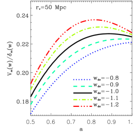
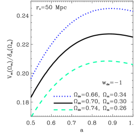
Figure 2: (Color online) The ratio $V_{\text{m}}/|\delta_{\text{m}}|$ for dark energy models with different values of EoS parameter (left-hand), with different values of density parameter $\Omega_{\text{de}}$ (central) and fixed zero spatial curvature ($\Omega_{\text{k}}=0$), with different values of density parameter $\Omega_{\text{de}}$ (right-hand) and fixed matter density parameter ($\Omega_{\text{m}}=0.3$). The dark energy perturbations have not been taken into account.

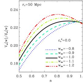
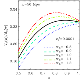
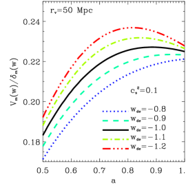
Figure 3: (Color online) The ratio $V_{\text{m}}/|\delta_{\text{m}}|$ for dynamical dark energy models with different values of effective sound speed. The dark energy perturbations have been taken into account.

The dark energy impacts the evolution of matter density and velocity perturbations in two ways. The first one is realised via the rate of expansion of the Universe: the equations (3.7)–(3.8) for matter density and velocity perturbations contain the function $H(a)$, equation (3.2), which depends on $\Omega_{\text{de}}$ and $w_{\text{de}}$. The second way consists in the impact of the density perturbations of dark energy on the evolution of matter density and velocity perturbations via the gravitational potential $\nu$, equation (3.6). The evolution of dark energy density and velocity perturbations, equations (3.7)–(3.8), depends on $\Omega_{\text{de}}$, $w_{\text{de}}$ and $c_{\text{s}}^{2}$. To estimate the level of the impact of dark energy on the ratio $V_{\text{m}}(r)/|\delta_{\text{m}}(r)|$ for dark matter we integrate the system of equations (3.6)–(3.8) in a simplified version ($\nu$, $\delta_{\text{m}}$, $v_{\text{m}}$, $\delta_{\text{rel}}$, $v_{\text{rel}}$) and a full version ($\nu$, $\delta_{\text{m}}$, $v_{\text{m}}$, $\delta_{\text{de}}$, $v_{\text{de}}$, $\delta_{\text{rel}}$, $v_{\text{rel}}$), without and with the density and velocity perturbations of dark energy.

In figure 2, we show the dependences of ratio $V_{\text{m}}(r)/|\delta_{\text{m}}(r)|$ on scale factor $a$ when the dark energy perturbations have not been taken into account. Here and below all dependences of this ratio on $a$ are computed for the point, which is at the distance $r=1.8$ Mpc from the central point of the void. In the left-hand panel we show the dependences of this ratio on scale factor $a$ for the models of dark energy with different values of equation of state parameter. One can see that the lines vary in slope and amplitude for different $a$. In the central and right-hand panels of figure 2 we show how the ratio $V_{\text{m}}(r)/|\delta_{\text{m}}(r)|$ depends on $a$ for different values of the dark energy density in the cosmological models with fixed zero spatial curvature ($\Omega_{\text{k}}=0$) and fixed matter density ($\Omega_{\text{m}}=0.3$), accordingly. In the case of fixed spatial curvature, the lines correlate with the value of $\Omega_{\text{m}}$ since the equality $\Omega_{\text{de}}+\Omega_{\text{m}}+\Omega_{\text{k}}=1$ is always true. The equations (3.6) and (3.8) explain this. When $\Omega_{\text{de}}$ and $\Omega_{\text{k}}$ are free parameters for fixed $\Omega_{\text{m}}$ (right-hand panel), the lines vary less, this illustrates the well-known degeneracy between these parameters. Since the Planck 2015 results state that $|\Omega_{\text{k}}|<0.005$ [66], the results in the right-hand panel have only a theoretical meaning. Therefore, we can state that the observational data on the ratio $V_{\text{m}}(r)/|\delta_{\text{m}}(r)|$ for the large voids can be used to constrain the values of density and equation of state parameters.

Let us integrate now the system of equations (3.6)–(3.8) in the complete version, when the solutions for all functions $\nu$, $\delta_{\text{m}}$, $v_{\text{m}}$, $\delta_{\text{de}}$, $v_{\text{de}}$, $\delta_{\text{rel}}$, $v_{\text{rel}}$ are sought. The amplitudes of density perturbations of dark energy at the late stages of evolution depend on the value of squared effective sound speed $c_{\text{s}}^{2}$ of dark energy. They are larger for lower $c_{\text{s}}^{2}$ [20]. The results show that the impact of dark energy perturbations on the matter ones is negligibly small for dark energy models with $c_{\text{s}}^{2}>0.01$. It is noticeable only for small values of the effective speed of sound. In figure 3 we show the dependences of the ratio $V_{\text{m}}(r)/|\delta_{\text{m}}(r)|$ on $a$ for $c_{\text{s}}^{2}=0,\,10^{-4},\,0.1$. One can see that the right-hand plot for $c^{2}_{\text{s}}$=0.1 does not practically differ from the left-hand plot in figure 2, where the perturbations of dark energy have not been taken into account at all. The maximal differences of ratios $V_{\text{m}}(r)/|\delta_{\text{m}}(r)|$ for the corresponding models in the left-hand panels of figures 2 and 3 are within 2–3 percent. So, the high accuracy data of future observations can be used for constraining $c_{\text{s}}^{2}$ from below.

Therefore, the observational data on structure of voids and peculiar velocities of galaxies in them at different redshifts can be used to distinguish the models of dark energy and determine their parameters. We understand that these results indicate only the sensitivity of void characteristics to the parameters of dark energy models for single spherical voids. Most of the real voids are non-spherical, surrounded by massive structures, while the galaxies and dark matter are biased. The impact of the form of the voids, their surroundings and galactic biasing can be taken into account on the basis of detailed $N$-body simulations of the formation of a large-scale structure of the Universe.

4 Conclusions

The voids as elements of a large-scale structure of the Universe have been studied intensively for almost forty years since their discovery. We have learned many interesting things about their origin, formation, properties and population, but many problems connected with them remain unsolved. Huge scientific activity in the world is connected with the dark energy — ‘‘the mystery of millennium’’, as Thanu Padmanabhan, renowned Indian theoretical physicist and cosmologist, said after publication of the results supporting apparently the viewpoint that something like cosmological constant is inherent for our Universe. Its nature remains unknown despite the tremendous efforts of theoretical physicists, cosmologists and astrophysicists to shed light into this dark kingdom. Probably, the combination of efforts in research of these two kinds of ‘‘darkness’’ will help us to understand the nature of both. The results presented here nourish this hope.

Ukrainian 0

Порожнини в космiчнiй павутинi як зонд темної енергiї

Б. Новосядлий, М. Цiж

             
Астрономiчна обсерваторiя, Львiвський нацiональний унiверситет iменi Iвана Франка,
вул. Кирила i Мефодiя, 8, 79005 Львiв, Україна

References

- [1] Eistein A., In: Sitzungsberichte der Königlich Preußischen Akademie der Wissenschaften, Berlin, 1917, 142–152.
- [2] Perlmutter S. et al., Astrophys. J., 1999, 517, 565; doi:10.1086/307221.
- [3] Riess A.G. et al., Astron. J., 1998, 116, 1009; doi:10.1086/300499.
- [4] Schmidt B.P. et al., Astrophys. J., 1998, 507, 46; doi:10.1086/306308.
- [5] Huterer D., Turner M.S., Phys. Rev. D, 1999, 60, 081301; doi:10.1103/PhysRevD.60.081301.
- [6] Amendola L., Tsujikawa S., Dark Energy: Theory and Observations, Cambridge University Press, Cambridge, 2010.
- [7] Lectures on Cosmology: Accelerated Expansion of the Universe, Wolschin G. (Ed.), Springer, Berlin, Heidelberg, 2010; doi:10.1007/978-3-642-10598-2.
- [8] Dark Energy: Observational and Theoretical Approaches, Ruiz-Lapuente P. (Ed.), Cambridge University Press, Cambridge, 2010.
- [9] Novosyadlyj B., Pelykh V., Shtanov Yu., Zhuk A., Dark Energy: Observational Evidence and Theoretical Models, Akademperiodyka, Kyiv, 2013.
- [10] Li B., Zhao H., Phys. Rev. D, 2009, 80, 044027; doi:10.1103/PhysRevD.80.044027.
- [11] Biswas R., Alizadeh E., Wandelt B.D., Phys. Rev. D, 2010, 82, 023002; doi:10.1103/PhysRevD.82.023002.
-
[12]
Bos E.G.P., van de Weygaert R., Dolag K., Pettorino V.,
Mon. Not. R. Astron. Soc., 2012, 426, 440;
doi:10.1111/j.1365-2966.2012.21478.x. - [13] Li B., Zhao G.-B., Koyama K., Mon. Not. R. Astron. Soc., 2012, 421, 3481; doi:10.1111/j.1365-2966.2012.20573.x.
- [14] Clampitt J., Cai Y.-C., Li B., Mon. Not. R. Astron. Soc., 2013, 431, 749; doi:10.1093/mnras/stt219.
- [15] Jennings E., Li Y., Hu W., Mon. Not. R. Astron. Soc., 2013, 434, 2167; doi:10.1093/mnras/stt1169.
- [16] Cai Y.-C., Padilla N., Li B., Mon. Not. R. Astron. Soc., 2015, 451, 1036; doi:10.1093/mnras/stv777.
- [17] Dai D.-C., Mon. Not. R. Astron. Soc., 2015, 454, 3590; doi:10.1093/mnras/stv2208.
-
[18]
Hamaus N., Sutter P.M., Lavaux G., Wandelt B.D.,
J. Cosmol. Astropart. Phys., 2015, 11, 036;
doi:10.1088/1475-7516/2015/11/036. - [19] Tsizh M., Novosyadlyj B., Adv. Astron. Space Phys., 2016, 6, 28; doi:10.17721/2227-1481.6.28-33.
- [20] Novosyadlyj B., Tsizh M., Kulinich Yu., Mon. Not. R. Astron. Soc., 2017, 465, 482; doi:10.1093/mnras/stw2767.
- [21] Bond J.R., Kofman L., Pogosyan D., Nature, 1996, 380, 603; doi:10.1038/380603a0.
- [22] Albert R., Barabasi A.L., Rev. Mod. Phys., 2002, 74, 47; doi:10.1103/RevModPhys.74.47.
- [23] Holovatch Yu., Olemskoi O., von Ferber C., Holovatch T., Mryglod O., Olemskoi I., Palchykov V., J. Phys. Stud., 2006, 10, 247.
- [24] Holovatch Yu., Kenna R., Thurner S., Preprint arXiv:1610.01002, 2016.
- [25] Gregory S.A., Thompson L.A., Astrophys. J., 1978, 222, 784; doi:10.1086/156198.
- [26] Joeveer M., Einasto J., Tago E., Mon. Not. R. Astron. Soc., 1978, 185, 357; doi:10.1093/mnras/185.2.357.
- [27] Zeldovich Ya.B., Einasto J., Shandarin S.F., Nature, 1982, 300, 407; doi:10.1038/300407a0.
- [28] Silk J., Szalay A.S., Zel’dovich Ya.B., Sci. Am., 1983, 249, No. 4, 56; doi:10.1038/scientificamerican1083-72.
- [29] Sato H., In: General Relativity and Gravitation, Bertotti B., de Felice F., Pascolini A. (Eds.), D. Reidel Publishing Company, Dordrecht, 1984, 289–312; doi:10.1007/978-94-009-6469-3_15.
- [30] Maeda K., Sasaki M., Sato H., Prog. Theor. Phys., 1983, 69, 89; doi:10.1143/PTP.69.89.
- [31] Fujimoto M., Astron. Soc. Jpn., 1983, 35, No. 2, 159.
- [32] Icke V., Mon. Not. R. Astron. Soc., 1984, 206, 1; doi:10.1093/mnras/206.1.1P.
- [33] Ryden B.S., Turner E.L., Astrophys. J., 1984, 287, L59; doi:10.1086/184398.
- [34] Vettolani G., de Souza R., Marano B., Chincarini G., Astron. Astrophys., 1985, 144, No. 2, 506.
- [35] Mao Q. et al., Preprint arXiv:1602.02771, 2016.
- [36] Pierre M., Shaver P.A., Iovino A., Astron. Astrophys., 1988, 197, L3.
- [37] Ostriker J.P., Bajtlik S., Duncan R.C., Astrophys. J., 1988, 327, L35; doi:10.1086/185135.
- [38] Dobrzycki A., Bechtold J., Astrophys. J., 1991, 377, L69; doi:10.1086/186119.
- [39] Stark C.W., Font-Ribera A., White M., Lee K.-G., Preprint arXiv:1504.03290, 2014.
- [40] Ouchi M. et al., Astrophys. J. Lett., 2005, 620, L1; doi:10.1086/428499.
- [41] Hamaus N., Sutter P.M., Wandelt B.D., Phys. Rev. Lett., 2014, 112, 251302; doi:10.1103/PhysRevLett.112.251302.
-
[42]
Colberg J.M., Sheth R.K., Diaferio A., Gao L., Yoshida N., Mon. Not. R. Astron. Soc., 2005, 360, 216;
doi:10.1111/j.1365-2966.2005.09064.x. -
[43]
Gottlöber S., Łokas E. L., Klypin A., Hoffman Y., Mon. Not. R. Astron. Soc., 2003,
344, No. 3, 715;
doi:10.1046/j.1365-8711.2003.06850.x. - [44] Arbabi-Bidgoli S., Müller V., Mon. Not. R. Astron. Soc., 2002, 332, 205; doi:10.1046/j.1365-8711.2002.05296.x.
- [45] Wojtak R., Powell D., Abel T., Mon. Not. R. Astron. Soc., 2016, 458, 4431; doi:10.1093/mnras/stw615.
- [46] Sutter P.M., Elahi P., Falck B., Mon. Not. R. Astron. Soc., 2014, 445, No. 2, 1235; doi:10.1093/mnras/stu1845.
- [47] Van de Weygaert R., Proc. Int. Astron. Union, 2016, 11, No. S308, 493; doi:10.1017/S1743921316010504.
- [48] Haque-Copilah S., Basu D., Publ. Astron. Soc. Pac., 1994, 106, No. 695, 67; doi:10.1086/133344.
-
[49]
Dubinski J., da Costa L.N., Goldwirth D.S., Lecar M., Piran T., Astrophys. J., 1993, 410, No. 2, 458;
doi:10.1086/172762. - [50] Van de Weygaert R., Sheth R.K., Preprint arXiv:astro-ph/0310914, 2003.
-
[51]
Sheth R.K., van de Weygaert R., Mon. Not. R. Astron. Soc., 2004, 350, No. 2, 517;
doi:10.1111/j.1365-2966.2004.07661.x. - [52] Ghigna S., Bonometto S., Retzlaff J., Gottloeber S., Murante G., Astrophys. J., 1996, 469, 40; doi:10.1086/177755.
-
[53]
Amendola L., Frieman J., Waga I., Mon. Not. R. Astron. Soc., 1999, 309, No. 2, 465;
doi:10.1046/j.1365-8711.1999.02841.x. -
[54]
Chantavat T., Sawangwit U., Sutter P.M., Wandelt B.D., Phys. Rev. D, 2016, 93, 043523;
doi:10.1103/PhysRevD.93.043523. - [55] Krause E., Chang T.-C., Doré O., Umetsu K., Astrophys. J. Lett., 2013, 762, L20; doi:10.1088/2041-8205/762/2/L20.
- [56] Alcock C., Paczyński B., Nature, 1979, 281, 358; doi:10.1038/281358a0.
- [57] Lavaux G., Wandelt B.D., Astrophys. J., 2012, 754, 109; doi:10.1088/0004-637X/754/2/109.
-
[58]
Sutter P.M., Pisani A., Wandelt B.D., Weinberg D.H., Mon. Not. R. Astron. Soc., 2014, 443, 2983;
doi:10.1093/mnras/stu1392. - [59] Neyrinck M., Mon. Not. R. Astron. Soc., 2008, 386, 2101; doi:10.1111/j.1365-2966.2008.13180.x.
- [60] Sutter P.M., Lavaux G., Hamaus N., Pisani A., Wandelt B.D., Warren M., Villaescusa-Navarro F., Zivick P., Mao Q., Thompson B.B., Astron. Comput., 2015, 9, 1; doi:10.1016/j.ascom.2014.10.002.
- [61] Nadathur S., Hotchkiss S., Diego J.M., Iliev I.T., Gottlöber S., Watson W.A., Yepes G., Proc. Int. Astron. Union, 2016, 11, No. S308, 342; doi:10.1017/S1743921316010541.
-
[62]
Ricciardelli E., Quilis V., Varela J., Proc. Int. Astron. Union, 2016, 11, No. S308, 551;
doi:10.1017/S1743921316010565. - [63] Li B., Mon. Not. R. Astron. Soc., 2011, 411, 2615; doi:10.1111/j.1365-2966.2010.17867.x.
- [64] Spolyar D., Sahlén M., Silk J., Phys. Rev. Lett., 2013, 111, 241103; doi:10.1103/PhysRevLett.111.241103.
- [65] Lavaux G., Wandelt B.D., Mon. Not. R. Astron. Soc., 2010, 403, 1392; doi:10.1111/j.1365-2966.2010.16197.x.
- [66] Planck Collaboration, Astron. Astrophys., 2016, 594, A13; doi:10.1051/0004-6361/201525830.
- [67] Riess A. et al., Astrophys. J., 2016, 826, 56; doi:10.3847/0004-637X/826/1/56.
- [68] Novosyadlyj B., Tsizh M., Kulinich Yu., Gen. Relativ. Gravitation, 2016, 48, 30; doi:10.1007/s10714-016-2031-8.
Ukrainian \adddialect\l@ukrainian0 \l@ukrainian