The effect of temperature on generic stable periodic structures in the parameter space of dissipative relativistic standard map

Abstract

In this work, we have characterized changes in the dynamics of a two-dimensional relativistic standard map in the presence of dissipation and specially when it is submitted to thermal effects modeled by a Gaussian noise reservoir. By the addition of thermal noise in the dissipative relativistic standard map (DRSM) it is possible to suppress typical stable periodic structures (SPSs) embedded in the chaotic domains of parameter space for large enough temperature strengths. Smaller SPSs are first affected by thermal effects, starting from their borders, as a function of temperature. To estimate the necessary temperature strength capable to destroy those SPSs we use the largest Lyapunov exponent to obtain the critical temperature ($T_{C}$) diagrams. For critical temperatures the chaotic behavior takes place with the suppression of periodic motion, although, the temperature strengths considered in this work are not so large to convert the deterministic features of the underlying system into a stochastic ones.

1 Introduction

The complex behavior of a charged particle in a field of a wave packet represents one of the fundamental problems envolving the theory of plasma physics and it has attracted attention for many years ll92 . One simple way to characterize such complex behaviors is the study of a discrete time version of differential equations used to model the motion of classical particles. A well know discrete time system or map used to describe the dynamics of a relativistic particle in a wave packet was originally proposed in Ref. ctvz89 , revisited in nih92 ; mmss05 and extended to dissipative regime in cbs02 . A natural question arises from this scenario when one intends to submit a dissipative relativistic particle to thermal effects modeled by Gaussian noise added to the system: what are the most common effects caused by noise in the periodic underlying dynamics of charged particles as function of temperature of thermal environment? As reported in Ref. lt11 there are two common phenomena induced by the influence of temperature or noise: (i) noise-induced chaos and (ii) noise-induced crisis. In (i) trajectory can visit the original periodic attractor (null noise) and the chaotic saddle, creating in this way an extended chaotic attractor; while in (ii) noise can cause trajectories on the attractor to move out of its basin of attraction. Actually, in the real world, classical particles always suffer environmental effects, such as noise or temperature, which give rise to new dynamical behaviors and therefore, requiring new comprehensive approach. Then, to explain such behaviors in nature and for technological applications, it is of fundamental priority to understand the effect of noise (thermal or not) on the resistence of periodic behaviors.

In the present work we revisit the investigation of nonlinear dynamics of a particle described by a dissipative relativistic standard map (DRSM), introduced by cbs02 and later explored in ly08 ; olr11 ; ol12 and, specially extend the study published by Oliveira and Leonel in the Ref. ol14 , where the authors investigated the statistical and dynamical behaviors for conservative and dissipative relativistic particles in waveguide. In order to understand and to describe the role of dissipation and relativistic parameters in the DRSM we perform extensive numerical investigations besides some few analytical analysis. In addition, we also characterize the main changes in the dynamics of such particles under the influence of a thermal environment. Our aim is to understand what happens with periodic and chaotic attractors when the relativistic particle is affected by a Gaussian stochastic signal for different temperature strengths. To this end we use the following numerical approaches: (i) calculate the Lyapunov spectra (to get the Largest Lyapunov Exponents (LLE)) based on Benettin’s algorithm bggs80 ; wssv85 , which includes the Gram–Schmidt re-orthonormalization procedure and, (ii) obtain the periods of trajectories for different pairs of parameters used to describe dynamical behaviors in two-dimensional diagrams (so called Lyapunov and isoperiodic diagrams, respectively) of the four-dimensional parameter-space of the discrete-time system. Besides, we also estimate the critical temperature needed to destroy the periodic attractors using the value of LLE.

We find that all possible considered two-dimensional diagrams present generic self-organized periodic structures embedded in a single chaotic domain, namely stable periodic structures (SPSs), well known to be typical or generic in dissipative nonlinear dynamical systems. Such kind of SPSs were found in a wide range of both, discrete and continuous time systems cmab11 ; cmab14 (and references therein), including ratchet systems, chemical reactions, population dynamics, electronic circuits, and laser models, among others. In addition, as far as we know, the resistance of SPSs as a function of temperature was recently characterized using the parameter planes dissipation versus ratchet parameter considering the presence of Gaussian noise in ratchet systems as can be found in the Ref. mcb13 .

In the following, we describe the organization of this paper. Starting with Sec. 2, we introduce the DRSM and some analytical results. Sec. 3 presents the numerical results (for null temperature case) that clearly show the influence of dissipation and relativistic parameters in the presence of generic SPSs embedded in a single chaotic domain. Results about extensive numerical experiments are discussed in Sec. 4 and they confirm the destruction of SPSs (starting from their borders) and large periodic domains when stochastic effects are considered for large enough temperature, remaining only the chaotic ones. Finally, in Sec. 5 we summarize and discuss our main conclusions.

2 The discrete time model

Based on the well known dissipative standard map ll92 the authors of Ref. cbs02 introduced a dissipative relativistic standard map (DRSM), that is a discrete time system described as a transformation onto the real plane to itself $f(x,y):\mathbb{R}^{2}\mapsto\mathbb{R}^{2}$, used to investigate the dynamics of a massive charged particle in the electric field of an electromagnetic wave packet. The main aim was describe how relativistic effects change the nonlinear dynamics presented by a dissipative standard map. The effects of the environment are taken into account in the DRSM dynamics through of a velocity-dependent dissipation and thermal fluctuations. In such case, the relativistic particle is placed at a Gaussian thermal bath giving the following map

$$\left\{\begin{array}[]{ll}y_{t+1}=\gamma y_{t}+\dfrac{K}{2\pi}\sin(2\pi x_{t})+\xi(t),\\ \\ x_{t+1}=x_{t}+{\dfrac{y_{t+1}}{\sqrt{1+(\beta y_{t+1})^{2}}}}\hskip 8.53581pt\mbox{mod}~{}1,\end{array}\right.$$ (4)

where $t=0,1,2,\ldots$ represents the discrete time, $y$ is the momentum variable conjugated to $x$, $K$ is the nonlinear parameter responsible for the transition from integrable motion ($K=0$) to chaotic dynamics ($K\neq 0$). The dissipation parameter $\gamma$ reaches the overdamping limit for $\gamma=0$ and the Hamiltonian-conservative limit for $\gamma=1$ and $\beta$ represents the relativistic parameter. In the limit of $\beta\rightarrow 0$ and $\gamma\rightarrow 1$ the relativistic standard map is reduced to Chirikov standard map. For $\beta=1$ the resonance case is reached and it was previously studied in the Ref. ly08 . The thermal noise represented by $\xi(t)$ is a stochastic variable obeying $\langle\xi(t)\rangle=0$ and the fluctuation-dissipation theorem that gives the relation between $\xi$ and $\gamma$ as $\langle\xi(t)^{2}\rangle=2(1-\gamma)k_{B}T$, with $k_{B}=1$ being the Boltzmann constant and $T$ the temperature.

2.1 A brief analytical analysis

Analytical boundaries for the SPSs in the two-dimensional parameter diagrams can be obtained for fixed points (period-1 attractors or orbits), as previously performed for a ratchet discrete-time system in Ref. cmab11 . Such boundaries are determined from the analytical expression for eigenvalues $\lambda(K,\beta,\gamma,N)$ obtained from Jacobian matrix of the map (4) after one iteration as described bellow.

The fixed points or period-1 attractors $(x^{*},y^{*})$ of Eq. (4) for $T=0$, are obtained after one iteration by solving the system

$$\left\{\begin{array}[]{ll}\sin(2\pi x^{*})=\dfrac{2\pi}{K}(\gamma-1)y^{*}\\ \\ x^{*}=\left(x^{*}+\dfrac{y^{*}}{\sqrt{1+(\beta y^{*})^{2}}}\right)\hskip 8.53581pt\mbox{mod}~{}1,\end{array}\right.$$ (8)

which after some algebraic manipulations result in the orbital solutions (fixed points coordinates in phase space) given by

$$\left\{\begin{array}[]{ll}y^{*}_{N}=\dfrac{N}{\sqrt{1-(N\beta)^{2}}},\\ \\ x^{*}_{N}=\dfrac{1}{2\pi}\arcsin\left[\dfrac{2\pi}{K}(\gamma-1)\dfrac{N}{\sqrt{1-(N\beta)^{2}}}\right],\end{array}\right.$$ (12)

where $N$ is an integer or rational number which results from the solution of second expression of Eq. (8) and, it is related to the position of respective fixed point in phase space. As a term under a square root must be positive to be real and the $|\sin(2\pi x^{*})|\leq 1$, we obtain the restrictions $|N|<1/\beta$ and $|(2\pi/K)(\gamma-1)N(1-(N\beta)^{2})^{-1/2}|\leq 1$, which is the reason for a finite number of fixed points in phase space.

Substituting the orbital solutions (12) in the Jacobian matrix of map (4) just after one iteration, we find the analytical expressions for two eigenvalues $\lambda(K,\beta,\gamma,N)$ as a function of system’s parameters and $N$. Setting one of these eigenvalues equal to $+1$ (for more details see Ref. gh83 ), we find where (and for which parameter sets) period-1 attractors are born in the phase-space. As the Jacobian matrix and eigenvalue expressions are very large they are not written explicitly here. So, using this procedure it is possible to obtain $K(\beta,\gamma,N)$ and $\beta(\gamma,K,N)$, which defines the boundaries in the two-dimensional parameter diagrams where period-1 attractors are born. In other words, the solution for equation $\lambda(K,\beta,\gamma,N)-1=0$ for one eigenvalue results in the following expression

$$K(\beta,\gamma,N)=\pm\frac{2\pi(\gamma-1)N}{\sqrt{1-N^{2}\beta^{2}}}.$$ (13)

Otherwise, if the eigenvalue equation is solved for $\beta$ in terms of $\gamma,K$ and $N$ one obtains

$$\beta(\gamma,K,N\neq 0)=\sqrt{\frac{K^{2}-4\pi^{2}(\gamma-1)^{2}N^{2}}{N^{2}K^{2}}}.$$ (14)

In summary, these expressions are very useful for allowing us to find position birth of the period-1 attractors in the ($K,\beta$) (or $\beta$,$\gamma$) two-dimensional Lyapunov or isoperiodic diagrams, respectively, as discussed in the next section (see Fig. 1(b)). An additional detailed discussion about a general procedure to find analytical expressions used to fit numerical boundaries between domains, characterized by different stable motions, in two-dimensional parameter space of generic two-dimensional dynamical systems can be found in Ref. g95 (see also references therein).

3 Numerical experiments for $T=0$

This Section is devoted to discuss the role of relativistic parameter $\beta$ in the dynamics of DRSM without the presence of thermal effects, i.e., $T=0$ in Eq. (4). We show the results applying numerical methods and analytical analysis. The numerical methods are based on the iteration of the map and obtain the two-dimensional diagrams for the largest Lyapunov exponent (Lyapunov diagram) ol12 ; mcms13 ; hsma14 ; srsab16 (see also references therein), and for the periods of the attractors (isoperiodic diagram) jg12 ; mepzgg16 ; g16 ; harmc16 as two parameters of the studied map are varied.

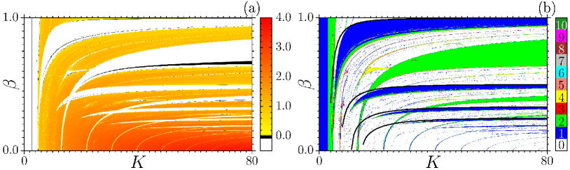
Figure 1: (a) The largest Lyapunov exponent (see color-bar) is plotted in the parameter-plane ($K,\beta$) for $\gamma=0.4$, while in (b) the periods for the same parameter-plane are plotted in colors (see color-bar), where the white color represents the larger periods than ten and chaotic attractors. The black-continuous curves fitting the fixed point domains (per-1 attractors) are the theoretical prevision given by Eq. (14) for $N=1,2,3$ and $4$.

The Lyapunov diagrams were obtained combining the set of parameters ${K,\gamma,\beta}$ taken two by two with the largest Lyapunov exponent being evaluated as the map is iterated. The graphic representation of the exponents is given by their magnitudes codified by color gradients. The white represents negative exponents (fixed points or period-1 attractors and higher-order periodic attractors), the black null exponents (bifurcations points) and continuously variation of yellow up to red for positive exponents (chaotic regions). The Lyapunov diagrams were obtained considering the discretization of the parameters in a grid of $1000\times 1000$ values, where a typical random initial condition (IC) given by $(x_{0},y_{0})=(0.1,0.3)$ was used to all parameter pairs. Some tests using different IC sets were performed and Lyapunov diagrams remain practically unchanged.

On the other hand, the isoperiodic diagrams also were obtained varying two of the set parameters ${K,\gamma,\beta}$ keeping the third constant in a grid of $1200\times 1200$ values of parameters, and iterating the map with the same initial conditions listed at the previous paragraph. In this calculations we discard $10^{7}$ iterations as transient time before the period of the attractor is evaluated for periods between $1$ up to $10$ plotted in the isoperiodic diagrams with a discrete color scheme. For periods greater than $10$ and chaotic attractors, the white color is associated. At this point becomes pertinent define an abbreviation for the period-$q$, where $q$ represents the period of attractor, shortly written as per-$q$, that is used along the text. Besides the numerical experiments we also use the analytical results discussed in Subsec. 2.1 to obtain the coordinates in the two-dimensional diagrams, where the per-$1$ attractors birth as a function of specific parameter pairs of DRSM.

In Figs. 1(a)-(b), we present the Lyapunov and Isoperiodic diagrams, respectively, for the Eq. (4) in the ($K,\beta$) two-dimensional diagrams. In Fig. 1(a), we observe a large chaotic region (from yellow up to red color) with embedded periodic windows. In Fig. 1(b), we observe that for the white structures in (a), that could be fixed points or periodic attractors, now they are blue (per-1 attractors), green (per-2 attractors), red (per-3 attractors), and so on up to dark-green (per-10 attractors), as indicated by color-bar at right in the isoperiodic diagram. As in the previous Subsection the white color represents both attractors with periods greater than $10$ or chaotic ones.

Comparing both Lyapunov and isoperiodic diagrams in Fig. 1(a) and (b) respectively, for $K$ values between $0$ and $5$ we observe in (a) a white strip that extending for $\beta$ values between $0.0$ and $1.0$ and it corresponds to a per-1 attractor (fixed point) and a per-2 attractor in (b) (see the blue and green colors inside that strip). Inside it there exist a period doubling bifurcation, where the bifurcation points are not completely visible in the Lyapunov diagram due to the numerical precision (see the thin black line in that last strip in (a)). Near to $K\sim 5$ and $\sim 12$ one can observe in (a) the birth of two large periodic strips (white color) that in (b) is a blue strip of per-1 and a green strip of per-2. From those two strips appear two distinct sequences of per-1 and per-2 strips with size decreasing, as $K$ increases and $\beta$ decreases.

We also plotted four curves, given by Eq. (14), for $N=1,2,3,4$ in Fig. 1(b), continuous-black lines bordered the first four per-1 structures (blue structures from top to bottom). These exemplary curves are composed by parameter pairs $(K,\beta)$ where the system (4) suffers boundary or exterior crisis bifurcations. It is worth to observe that those black lines, that mark where the fixed points or per-1 structures born, do not completely fit those structures in their left bottom side. This feature is related to the choice of the initial conditions used to iterate the map, i.e., the used initial condition gave rise to an attractor near that analytically evaluated by Eq. (14). However, it is difficult to choose initial conditions that exactly give rise to the same results found analytically. One can also see that four curves abruptly finish at left-hand side of same figure. This happens because exactly in the point where the root of Eq. (14) becomes negative, i.e., the function $\beta(K,\gamma,N)$ becomes imaginary and our theoretical prediction is inappropriate. Besides, it is possible to obtain curves for $N>4$, but the results are not easily visible in the present two-dimensional diagrams because the figures resolution.

In the next, a numerical description of the DRSM is carry out, emphasizing the relativistic parameter $\beta$. For this purpose some Lyapunov diagrams are constructed, as described in the beginning of Section 3. In Fig. 2 we show four Lyapunov diagrams for the $(K,\gamma)$ plane, varying the parameter $\beta$. In those four diagrams, the magnitude of the largest Lyapunov exponent follows the codification presented in the color-bar at right in diagram (d). For a small $\beta$ in Fig. 2(a), we observe a periodic region (white and black color) at the left side of the diagram and finished at the top. In addition, we also observe the presence of some thin strips (white and black color) that cross the chaotic region (yellow and red region) in the diagonal.

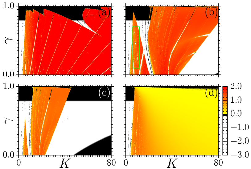
Figure 2: The largest Lyapunov exponent (see color-bar) is plotted in the parameter-plane ($K,\gamma$) for (a) $\beta=0.1$, (b) $\beta=0.4$, (c) $\beta=0.7$, and (b) $\beta=1$ (ressonant case).

In Fig. 2(b), a large periodic region (see black and white colors in color-bar) was born at right of the diagram, confining the chaotic behavior into two regions. Increasing the $\beta$ parameter, in Fig. 2(c), we note the shrinkage of the chaotic regions dominated by the periodic region at right. In the resonant case, $\beta=1$ in Fig. 2(d), the behavior previously observed, i.e., the increase of the periodic region at right in the diagrams, changes drastically, with the increase of the chaotic domain (yellow region) destroying the periodic domain at right of the diagram. It is also worth to note the periodic domain at the left of the diagrams of Fig. 2, that extending from $\gamma=0$ up to $\gamma=1$. That region practically remains unchanged for all values of $\beta$ used in the numerical simulations.

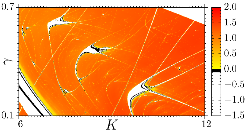
Figure 3: Magnification of Fig. 2(b) highlighted by green box and showing typical shrimp-shaped domains.

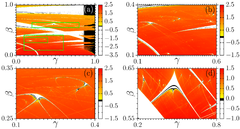
Figure 4: The largest Lyapunov exponent (see color-bar) is plotted in the parameter-plane ($\gamma,\beta$) for $K=20$. Figures (b-d) are magnifications of boxes plotted in (a).

Inside the chaotic domains of the diagrams in Fig. 2, we note some specific SPSs in addition to the thin strips discussed above. To clarify this, we magnified the region enclosed to the green box in Fig. 2(b), and show in Fig. 3, Lyapunov diagram of that domain: three cmab11 ; cmab14 ; fpg13 large SPSs are clearly observed. In special, the typical SPS located in the right-bottom side of Fig. 3 (about $(K,\gamma)\sim(9.5,0.25)$) is commonly known as shrimp-shaped robust isomorphic domain (as named by Gallas g93 ) or just shrimp-shaped domain. This kind of SPS is formally defined by the authors of Ref. vgg11 in terms of superstable parabolic arcs (whose definition is given for one-dimensional maps and recently extended for the dissipative Hénon map in Ref. fog13 through of numerical continuation methods). Another interesting definition for such generic SPSs, named compound windows and, also characterized in parameter space of dissipative Hénon map as performed in g93 , was introduced in 2008 by E. Lorenz l08 . According to Lorenz, compound windows are periodic windows which have a typical shape and consist of a central main “body” from which four narrow “antennae” extend. They are organized in bands which is known as window streets. We have been considered such definition in the discussion of our results, although, along the text we have been used the expression shrimp-shaped domain. As confirmed by a set of numerical experiments (magnifications not shown here), in some specific portions of parameter space of DRSM there are a large number of them. As a matter of fact, as we enlarged small portion of chaotic regions, further smaller typical shrimp-shaped domains are found g93 ; ol11 . As far as we know, the shrimp-shaped domain also is known as fishhook, since 1982 by Fraser and Kapral fk82 , for discrete maps and flows. In addition, it has been called by different names in the proper literature as, by instance, swallow mh89 and, crossroad area cmbst91 .

The black lines inside the shrimp-shaped domains are lines of bifurcation, once that null largest Lyapunov exponents refer to the bifurcations points of the map. As it was reported previously in Ref. hsma13 (see also references therein) the route to chaos, from inside of a shrimp-shaped domain to the chaotic region in specific directions, follows successive period-doubling bifurcations. More information about bifurcation theory and several robust results can be found in the Ref. m87 .

The Lyapunov diagrams for the $(\gamma,\beta)$ plane, with $K=20$, are shown in Fig. 4, where in (a) a large view is plotted while in (b)-(d) magnifications are presented for regions delimited by greens boxes in (a). In Fig. 4(a) large periodic strips (black-white strips) are seen in the diagram, and those strips extend along the chaotic region. Such strips represent fixed points (per-1 attractors) for each pair of $(\gamma,\beta)$ parameters represented by white color while black color is associated to bifurcation points (null largest Lyapunov exponent). In addition, as showed in Fig. 1(b), the upper boundaries of those strips are analytically fitted by Eq. (14), with $K$ fixed. In Fig. 4(b)-(d), three emblematic types of isomorphic periodic structures embedded in the chaotic region, as reported in some recent works about maps cmab11 ; g93 ; ol11 and flows hsma14 ; hsma13 and discussed in the previous paragraph are observed. Two of them, observed in Fig. 4(b), and better visualized in Fig. 4(c), are the well-known shrimp-shaped domains, at left-bottom side of the diagram, while at the right-top side of the diagram, a smaller set of three connected SPSs. Similar structures were recently reported in Ref. fpg13 for flows. The third one, shown in Fig. 4(d), is the cuspidal SPSs cmab14 ; g95 , sometimes also known as saddle area bst98 and rigorously demonstrated since 1985 as published in  g91 . A more comprehensive and didactical explanation about cuspidal SPSs can be found on appendix of Ref. gsv13 . Those Lyapunov diagrams also present self-affinity features, i.e., those SPSs appear in smaller scales of the Lyapunov diagrams.

The second set of partial conclusions is based on the rich and complex dynamics presented by DRSM, even without the presence of thermal effects, when two control parameter are varied simultaneously. Therefore, the high-complex configuration observed in the two-dimensional diagrams as discussed in this section is possible due to the features of self-similarities and affinities besides the evident proofs of existence of typical SPSs as, shrimp-shaped and cuspidal domains, which are believed generic in the parameter-spaces of nonlinear dynamical systems.

4 Using thermal effects ($T>0$) to perturb periodic attractors

In this Section the thermal effects are studied when the DRSM model is added by a Gaussian noise, as described by Eq. (4). Lyapunov diagrams were constructed for the $(K,\gamma)$ and $(\gamma,\beta)$ planes with $T$.

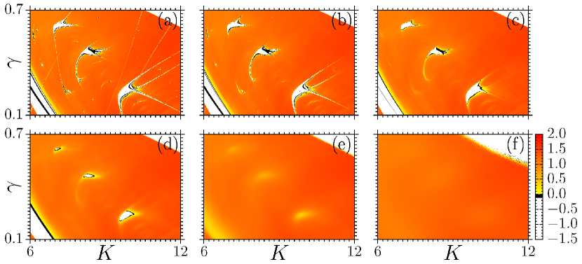
Figure 5: The largest Lyapunov exponent (see color-bar) is plotted in the parameter-plane $(K,\gamma)$ with $\beta=0.4$ for (a) $T=10^{-7}$, (b) $T=10^{-6}$, (c) $T=10^{-5}$, (d) $T=10^{-4}$, (e) $T=10^{-2}$, and (f) $T=10^{-1}$. As temperature increases the destruction of SPSs becomes more and more evident.

In Fig. 5, the Lyapunov diagrams as $T$ increases from $10^{-7}$ in (a), up to $10^{-1}$ in (f), are shown for $(K,\gamma)$. Fig. 3 presents the $T=0$ case. Comparing both cases, $T=0$ (Fig. 3) with $T=10^{-7}$ (Fig. 5(a)), considered very small temperature, minimal changes are observed. Mainly, in the chaotic region, very small periodic structures were destroyed, and some branches of the bigger SPSs became thin. More increasing the temperature, Figs. 5(b)-(d), this effect becomes more clear, all smaller SPSs embedded in the chaotic region are destroyed, just surviving the three largest, but the temperature effect also destroyed their branches, surviving only the core of the structures. In Figs. 5(e)-(f), the temperature achieves a critical condition where the periodic structures were completely destroyed. It is worth to note the “scars” that the periodic structures leave in the chaotic region when the temperature effects increase. For example, see in Figs. 5(c)-(e), the yellowish regions where before there were branches and pieces of periodic structures for low values of temperatures (Figs. 5(a)-(b)). Those pronounced scars (yellow scars in Fig. 5(e)) are a kind of “memory” in the dynamics of the map due to the existence of the periodic structures. These “memories” can be completely destroyed for higher values of temperatures (see Figs. 5(f)).

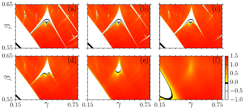
Figure 6: The largest Lyapunov exponent (see color-bar) is plotted in the parameter-plane $(\gamma,\beta)$ with $K=20$ for (a) $T=10^{-7}$, (b) $T=10^{-6}$, (c) $T=10^{-5}$, (d) $T=10^{-4}$, (e) $T=10^{-3}$, and (f) $T=10^{-2}$. As temperature increases the destruction of SPSs becomes more and more evident.

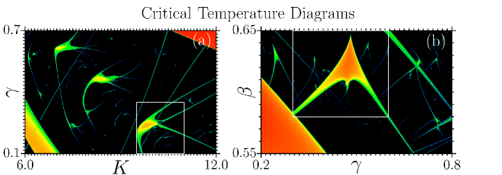
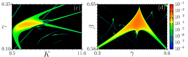
Figure 7: Plot of critical temperature $T_{C}$ (see the color-bar in (d)) necessary to destroy the SPSs in the (a) $(K,\gamma)$ plane, (b) $(\gamma,\beta)$ plane, and in the (c) and (d), magnifications of boxes in (a) and (b), respectively.

In Fig. 6, the Lyapunov diagrams, as $T$ increases from $10^{-7}$ in (a) up to $10^{-2}$ in (f), are shown for $(\gamma,\beta)$. The same behaviors presented previously in Fig. 5, are also observed in Fig. 6. The size of the structures in parameter space has a fundamental role in their stabilities regarding the temperature effects. Although the entire parameter space is perturbed by considering the presence of thermal effects in the system the smallest SPSs are more sensitive to the temperature strength, and they are the first to be destroyed if compared to the larger ones.

In the next we follow using the LLE to obtain the critical temperatures $T_{C}$ of the entire structure for which it will survive. For temperatures higher than its $T_{C}$, the whole periodic structures will be destroyed by thermal effects. In Fig. 7, we show the critical temperature diagrams for the $(K,\gamma)$ and $(\gamma,\beta)$ planes. $T_{C}$ is codified by the color-bar in a logarithmic scale. The diagrams of Figs. 7(a) and (b) are the same regions of Figs. 5(a) and. 6(a), respectively. Figures 7(c) and (d) are magnifications of the boxes in (a) and (b), respectively. It is clearly observed that $T_{C}$ is larger inside the structures, especially inside their inner parts. Thus, the periodic structures can still be recognized in such $T_{C}$ analysis. Even though $T_{C}$ is larger inside the inner parts of the structures, it tends to decrease at their borders. The procedure to obtain $T_{C}$ follows: for each pair of parameters, $(K,\gamma)$ or $(\gamma,\beta)$, $T$ in Eq. (4) was increased until the LLE reached positive values within the precision $10^{-3}$, which is a value below the minimum LLE allowed by the periodic constraints in the structures. Other precision values were tested and the main findings remain unchanged. It is possible to observe that the far from zero LLE in the chaotic region is independent of the parameters $(K,\gamma)$, or $(\gamma,\beta)$, within the precision $10^{-3}$. This defines the critical temperature $T_{C}$, where the near to zero LLE, due to periodic motion (inside the periodic structures), is transformed into the far from zero LLE due to the chaotic motion. By the $T_{C}$ analysis, we corroborate the assumption that how bigger is the SPS in the parameter-space, more resistant to destruction by thermal noise is the SPS.

We finish this Section stating the following conclusion: In the presence of a thermal reservoir, modeled by Gaussian noise, generic SPSs (as discussed above) usually are destroyed, starting from their borders, for large enough temperature and, characterizing this behavior as generic in parameter space. In addition, our results confirm that smaller SPSs are first affected by small thermal effects ($T\rightarrow 0$).

5 Summary and conclusions

The dissipative relativist standard map (DRSM) with Gaussian noise, Eq. (4), was numerically studied in this work. The Gaussian noise represents the thermal effect in the dynamics of the DRSM model. We start the numerical investigations of DRSM without the presence of noise obtaining the Lyapunov and isoperiodic diagrams for the dissipation parameter $\gamma$ and relativistic parameter $\beta$ besides the kicking strength $K$ and in this way we extend the previous investigation performed in Ref. ol14 . The birth of period-1 structures in the $(K,\beta)$ plane was also analytically obtained and numerically corroborated in the Lyapunov and isoperiodic diagrams. All the parameter-planes of the DRSM model present isomorphism regarding the presence of generic periodic structures embedded in the chaotic domains, also known as shrimp-shaped stable periodic structures (SPSs).

In a recent work mcb13 the thermal effect was studied in a discrete and continuous ratchet models and the critical temperature $T_{C}$ necessary to destroy the SPSs was obtained by the computation of the classical ratchet currents in the parameter-spaces. The authors showed that the SPSs are structures with optimal ratchet currents and how bigger these structures are in the parameter-space, more resistant to be destroyed by thermal effects they are. There is also the Ref. bsmcps15 , where the authors present results about quantum ratchet currents that inside the SPSs have been shown to be resistant to reasonable temperatures and to vacuum fluctuations. For some specific parameter combinations however, temperature and vacuum fluctuations induced ratchet currents. Now here, our numerical results clearly show that when a typical dynamical system is perturbed by temperature effects, SPSs immersed in chaotic domains usually are destroyed starting from their borders (antennae). To estimate the noise strength necessary to destroy SPSs, we propose a new numerical method to obtain the critical temperature $T_{C}$ by the computation of the largest Lyapunov exponents in the parameter-planes of the DRSM model, Eq. (4). It is very important to emphasize the power of this technique that can be applied to obtain $T_{C}$ using the largest Lyapunov exponent in any system models in contact with thermal reservoirs, where chaotic and periodic behaviors coexist for different parameter sets. To corroborate with this discussion, the information about $T_{C}$ is very relevant to show how robust are the SPSs in the presence of external perturbations as thermal effects. In the limit of sufficient small temperatures one can also applies this procedure to time series and estimate the strength of noise capable to destroy periodic behaviors in real experiments. In this case the chaotic characteristics of a deterministic dynamical system can be preserved as is often in experimental situations.

Author contributions

H.A.A. and C.M. conceived the simulations. A.C.C.H. and C.M. performed the simulations and all authors discussed the results. H.A.A. and C.M. wrote the manuscript.

References

- (1) A.J. Lichtenberg, M.A. Lieberman, Regular and Chaotic Dynamics (Springer-Verlag, New York, 1992)
- (2) A.A. Chernikov, T. Tél, G. Vattay, G.M. Zaslavsky, Phys. Rev. A 40, 4042 (1989)
- (3) Y. Nomura, H. Ichikawa, W. Horton, Phys. Rev. A 45, 1103 (1992)
- (4) D.U. Matrasulov, G.M. Milibaeva, U. Salomov, B. Sundaram, Phys. Rev. E 72, 016213 (2005)
- (5) C. Ciubotariu, L. Badelita, V. Stancu, Chaos Solitons & Fractals 13, 1253 (2002)
- (6) Y.C. Lai, T. Tél, Transient chaos (Springer, 2011)
- (7) B.L. Lan, C. Yapp, Chaos Solitons & Fractals 37, 1300 (2008)
- (8) D.F.M. Oliveira, E.D. Leonel, M. Robnik, Phys. Lett. A 375, 3365 (2011)
- (9) J.A. Oliveira, E.D. Leonel, Int. J. Bif. Chaos 22, 1250248 (2012)
- (10) D.F.M. Oliveira, E.D. Leonel, Physica A 413, 493 (2014)
- (11) G. Benettin, L. Galgani, A. Giorgilli, J.M. Strelcyn, Meccanica 15(9), 09 (1980)
- (12) A. Wolf, J.B. Swift, H.L. Swinney, J.A. Vastano, Physica D 16, 285 (1985)
- (13) A. Celestino, C. Manchein, H.A. Albuquerque, M.W. Beims, Phys. Rev. Lett. 106, 234101 (2011)
- (14) A. Celestino, C. Manchein, H.A. Albuquerque, M.W. Beims, Commun. Nonlinear Sci. Numer. Simulat. 19, 139 (2014)
- (15) C. Manchein, A. Celestino, M.W. Beims, Phys. Rev. Lett. 110, 114102 (2013)
- (16) J. Guckenheimer, P. Holmes, Nonlinear Oscillations, Dynamical Systems, and Bifurcations of Vector Fields, Vol. 42 of Applied Mathematical Sciences, 5th edn. (Springer-Verlag, New York, 1983)
- (17) J.A.C. Gallas, Physica A 222, 125 (1995)
- (18) E.S. Medeiros, R.O. Medrano-T., I.L. Caldas, L.T. Souza, Phys. Lett. A 377, 628 (2013)
- (19) A. Hoff, J.V. dos Santos, C. Manchein, H.A. Albuquerque, Eur. Phys. J. B 87, 151 (2014)
- (20) F.F.G. de Sousa, R.M. Rubinger, J.C. Sartorelli, H.A. Albuquerque, M.S. Baptista, Chaos 26, 083107 (2016)
- (21) L. Junges, J.A.C. Gallas, Phys. Lett. A 376, 2109 (2012)
- (22) R. Meucci, S. Euzzor, E. Pugliese, S. Zambrano, M.R. Gallas, J.A.C. Gallas, Phys. Rev. Lett. 116, 044101 (2016)
- (23) J.A.C. Gallas, in Advances in Atomic, Molecular, and Optical Physics, edited by E. Arimondo, C.C. Lin, S.F. Yelin (Elsevier Science, 2016), Vol. 65, chap. 3, pp. 127–191
- (24) A. L’Her, P. Amil, N. Rubido, A.C. Martí, C. Cabeza, Eur. Phys. J. B 89, 81 (2016)
- (25) R.E. Francke, T. Pöschel, J.A.C. Gallas, Phys. Rev. E 87, 042907 (2013)
- (26) J.A.C. Gallas, Phys. Rev. Lett. 70, 2714 (1993)
- (27) R. Vitolo, P. Glendinning, J.A.C. Gallas, Phys. Rev. E 84, 016216 (2011)
- (28) W. Façanha, B. Oldeman, L. Glass, Phys. Lett. A 377, 1264 (2013)
- (29) E. Lorenz, Physica D 237, 1689 (2008)
- (30) D.F.M. Oliveira, E.D. Leonel, Chaos 21, 043122 (2011)
- (31) S. Fraser, R. Kapral, Phys. Rev. A 25, 3223 (1982)
- (32) M. Markus, B.Hess, Comp. & Graph. 13, 553 (1989)
- (33) J.P. Carcassés, C. Mira, M. Bosh, C. Simó, J.C. Tatjer, Int. J. Bif. Chaos 1, 183 (1991)
- (34) A. Hoff, D.T. da Silva, C. Manchein, H.A. Albuquerque, Phys. Lett. A 378, 171 (2013)
- (35) C. Mira, Chaotic Dynamics (World Scientific, Singapore, 1987)
- (36) H. Broer, C. Simó, J.C. Tatjer, Nonlinearity 11, 667 (1998)
- (37) S.V. Gonchenko, Selecta Math. Soviet. 10, 69 (1991), a translation of Methods of Qualitative Theory of Differential Equations; pages 55-72, Ed. Gorky St. Univ., 1985.
- (38) S.V. Gonchenko, C. Simó, A. Vieiro, Nonlinearity 26, 621 (2013)
- (39) M.W. Beims, M. Schlesinger, C. Manchein, A. Celestino, A. Pernice, W.T. Strunz, Phys. Rev. E 91, 052908 (2015)