The projective ensemble and distribution of points in odd–dimensional spheres

Abstract.

We define a determinantal point process on the complex projective space that reduces to the so–called spherical ensemble for complex dimension $1$ under identification of the $2$–sphere with the Riemann sphere. Through this determinantal point process we propose a point processs in odd-dimensional spheres that produces fairly well–distributed points, in the sense that the expected value of the Riesz $2$–energy for these collections of points is smaller than all previously known bounds.

1. Introduction

Given $s\in(0,\infty)$, the Riesz $s$–energy of a set on points $\omega_{n}=\{x_{1},\ldots,x_{n}\}$ on a subset $X\subseteq\mathbb{R}^{m}$ is

(1) $$\mathcal{E}_{s}(\omega_{n})=\displaystyle\sum_{i\neq j}\frac{1}{\|x_{i}-x_{j}\|^{s}}.$$

This energy has a physical interpretation for some particular values of $s$, i.e. for $s=1$ the Riesz energy is the Coulomb potential and for $s=d-2$ ($d\geq 3$) is the Newtonian potential. In the special case $s=0$ the energy is defined by

$$\mathcal{E}_{0}(\omega_{n})=\left.\frac{d}{ds}\right|_{s=0}\mathcal{E}_{s}(\omega_{n})=\sum_{i\neq j}\log\|x_{i}-x_{j}\|^{-1}$$

and is related to the transfinite diameter and the capacity of the set by classical potential theory, see for example [doohovskoy2011foundations].

The minimal value of this energy and its asymptotic behavior have been extensively studied, most remarkably in the case that $X=\mathbb{S}^{d}\subseteq\mathbb{R}^{d+1}$ is the $d$–dimensional unit sphere. In [10.2307/117605] it was proved that for $d>2$ and $0<s<d$ there exist constants $c>C>0$ (depending only on $d$ and $s$) such that

(2) $$-cn^{1+\frac{s}{d}}\leq\min_{\omega_{n}}\left(\mathcal{E}_{s}(\omega_{n})\right)-V_{s}(\mathbb{S}^{d})n^{2}\leq-Cn^{1+\frac{s}{d}},$$

where $V_{s}(\mathbb{S}^{d})$ is the continuous s-energy for the normalized Lebesgue measure,

(3) $$V_{s}(\mathbb{S}^{d})=\frac{1}{Vol(\mathbb{S}^{d})^{2}}\displaystyle\int_{p,q\in\mathbb{S}^{d}}\frac{1}{\|p-q\|^{s}}dpdq=2^{d-s-1}\frac{\Gamma\left(\frac{d+1}{2}\right)\Gamma\left(\frac{d-s}{2}\right)}{\sqrt{\pi}\Gamma\left(d-\frac{s}{2}\right)}.$$

Finding the precise value of the constants in (2) is an important open problem and has been addressed by several authors, see [BHS2012b, Sandi, LB2015, MR1306011] for some very precise conjectures and [Brauchart2015293] or [BHSlibro] for surveys. One can post the problem as follows

Problem 1.1.

For $s\in(0,d)$, let $C_{s,d,n}$ be defined by

$$0<C_{s,d,n}=\frac{V_{s}(\mathbb{S}^{d})n^{2}-\min_{\omega_{n}}\left(\mathcal{E}_{s}(\omega_{n})\right)}{n^{1+\frac{s}{d}}}.$$

Find asymptotic values for $C_{s,d,n}$ as $n\to\infty$. In particular, prove if the limit exists.

A sometimes successful strategy for the upper bound in the constant $C_{s,d,n}$ is to take collections of random points in $\mathbb{S}^{d}$ and then compute the expected value of the energy (which is of course greater than or equal to the minimum possible value). Simply taking $n$ points with the uniform distribution in $\mathbb{S}^{d}$ already gives the correct term $V_{s}(\mathbb{S}^{d})n^{2}$, and other distributions with nice separation properties have proved successful in bounding the constant $C_{s,d,n}$.

We are thus interested in computationally feasible random procedures to generate points in sets which exhibit local repulsion. One natural choice is using determinantal point processes which have these two properties (see [Hough_zerosof] for theoretical properties and [PhysRevE.79.041108] for an implementation). A brief summary of the fundamental properties of determinantal point processes is given in Section 2.

In a recent paper [EJP3733] a determinantal point process named the spherical ensemble is used to produce low–energy random configurations on $\mathbb{S}^{2}$. This process was previously studied by Krishnapur [krishnapur2009] who proved a remarkable fact: the spherical ensemble is equivalent to taking eigenvalues of $A^{-1}B$ (where $A,B$ have Gaussian entries) and sending them to the sphere through the stereographic projection.

In [BMOC2015energy] a different determinantal point process rooted on the use of spherical harmonics is described, producing low–energy random configurations in $\mathbb{S}^{d}$ for some infinite sequence of values of $n$. In particular, it is proved in that paper that

(4) $$\limsup_{n\to\infty}C_{s,d,n}\geq 2^{s-s/d}V_{s}(\mathbb{S}^{d})\frac{d\,\Gamma\left(1+\frac{d}{2}\right)\Gamma\left(\frac{1+s}{2}\right)\Gamma\left(d-\frac{s}{2}\right)}{\sqrt{\pi}\Gamma\left(1+\frac{s}{2}\right)\Gamma\left(1+\frac{s+d}{2}\right)\left(d!\right)^{1-\frac{s}{d}}},\quad 0<s<d.$$

If $d-1<s<d$, $\limsup$ can be changed to $\liminf$ in (4) (see [BMOC2015energy, Cor. 2]). The bound in (4) is the best known to the date for general $d$ (although more precise bounds exist for particular values of $d$ including $d=1,2$, see [BLMS:BLMS0621, LB2015]). In particular, for $s=2$ and odd dimensions the formula in (4) reads

(5) $$\limsup_{n\to\infty}C_{2,2d+1,n}\geq\frac{2^{1-\frac{2}{2d+1}}\left({(2d+1)!}\right)^{\frac{2}{2d+1}}}{(2d-1)(2d+3)}\stackrel{{\scriptstyle d\to\infty}}{{\to}}\frac{2}{e^{2}}.$$

The determinantal point process in [BMOC2015energy] is called the harmonic ensemble and it is shown to be the optimal one (at least for $s=2$) among a certain class of determinantal point processes obtained from subspaces of functions with real values defined in $\mathbb{S}^{d}$.

However, the bound in [BMOC2015energy] for the case $d=2$ is worse than that of [EJP3733], which is not surprising since the spherical ensemble uses complex functions and is thus of a different nature.

An alternative natural interpretation of Krishnapur’s result is to consider eigenvalues $(\alpha,\beta)\in\mathbb{P}(\mathbb{C}^{2})$ of the generalized eigenvalue problem $\det(\beta A-\alpha B)=0$ and to identify $\mathbb{P}(\mathbb{C}^{2})$ with the Riemann sphere. An homotety then generates the points in the unit sphere $\mathbb{S}^{2}$. This remark suggests that the spherical ensemble can be seen as a natural point process in the complex projective space, and a search for an extension to higher dimensions is in order. In this paper we extend this process in a very natural manner to $\mathbb{P}(\mathbb{C}^{d+1})$ for any $d\geq 2$. We will propose the name projective ensemble.

In order to show the separation properties of the projective ensemble we will define a (probably non–determinantal) point process in odd–dimensional spheres, which will allow us to compare our results to those of [BMOC2015energy]. This point process is as follows: first, choose a number $r$ of points in $\mathbb{P}(\mathbb{C}^{d+1})$ coming from the projective ensemble. Then, consider $k$ equally spaced unit norm affine representatives of each of the projective points. We allow these points to be rotated by a randomly chosen phase. As a result, we get $rk$ points in the odd–dimensional sphere $\mathbb{S}(\mathbb{C}^{d+1})\equiv\mathbb{S}^{2d+1}$.

We study the expected $2$–energy of such a point process. Our first main result can be succinctly written as follows.

Theorem 1.2.

With the notations above,

(6) $$\begin{split}&\limsup_{n\to\infty}C_{2,2d+1,n}\geq\frac{3^{1-\frac{2}{2d+1}}(2d-1)^{1-\frac{2}{2d+1}}(2d+1)\Gamma\left(d-\frac{1}{2}\right)^{2-\frac{2}{2d+1}}}{2^{4-\frac{2}{2d+1}}(d!)^{2-\frac{4}{2d+1}}}\stackrel{{\scriptstyle d\to\infty}}{{\to}}\frac{3}{4e}.\end{split}$$

The bound in Theorem 1.2 is larger than that of (5), which shows that random configurations of points coming from this point process are, at least from the point of view of the $2$–energy, better distributed than those coming from the harmonic ensemble. See Figure 1 for a graphical comparison of both bounds.

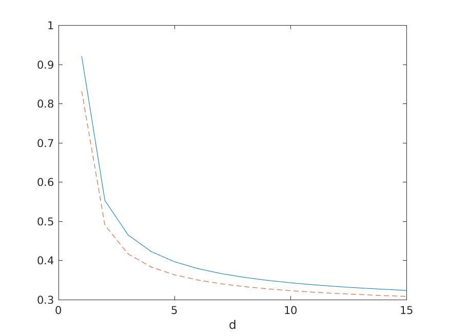
Figure 1. Comparison of the values of the constants in (6) (blue solid line) and (5) (red dashed line).

Since the point process we have defined in $\mathbb{S}^{2d+1}$ starts by choosing points in $\mathbb{P}(\mathbb{C}^{d+1})$ coming from the projective ensemble, Theorem 1.2 gives us arguments to think that the projective ensemble produces quite well distributed points in $\mathbb{P}(\mathbb{C}^{d+1})$ (for $d=1$ this property is quantitatively described in [EJP3733]). There are several ways to measure how well distributed a collection of points is in $\mathbb{P}(\mathbb{C}^{d+1})$. For example, one can study the natural analogues of Riesz’s energy as in Theorem 3.3 below. A very natural measure is given by the value of Green’s energy of [Juan]: let $G:\mathbb{P}(\mathbb{C}^{d+1})\times\mathbb{P}(\mathbb{C}^{d+1})\to[0,\infty]$ be the Green function of $\mathbb{P}(\mathbb{C}^{d+1})$, that is, $G(x,\cdot)$ is zero–mean for all $x$, $G$ is symmetric and $\Delta_{y}G(x,y)=\delta_{x}(y)-vol(\mathbb{P}(\mathbb{C}^{d+1}))^{-1}$, with $\delta_{x}$ the Dirac’s delta function, in the distributional sense. The Green energy of a collection of $r$ points $\omega_{r}=(x_{1},\ldots,x_{r})\in\mathbb{P}(\mathbb{C}^{d+1})^{r}$ is defined as

$$\mathcal{E}_{G}(\omega_{r})=\sum_{i\neq j}G(x_{i},x_{j}).$$

Minimizers of Green’s energy are assymptotically well–distributed (see [Juan, Main Theorem]). Our second main result will follow from the computation of the expected value of Green’s energy for the projective ensemble.

Theorem 1.3.

Let $d\geq 2$. Then,

(7) $$\liminf_{r\to\infty}\frac{\min_{\omega_{r}}\left(\mathcal{E}_{G}^{\mathbb{P}}(\omega_{r})\right)}{r^{2-\frac{1}{d}}}\leq-\frac{(d!)^{1-\frac{1}{d}}}{4\pi^{d}(d-1)}.$$

Theorem 1.3 gives a criterium to decide how well–distributed a collection of projective points is: compute their Green’s energy and compare to that of (7).

2. Determinantal point processes

2.1. Basic notions

In this section we follow [Hough_zerosof].

Definition 2.1.

Let $\Lambda$ be a locally compact, polish topological space with a Radon measure $\mu$. A simple point process $\mathfrak{X}$ of $n$ points in $\Lambda$ is a random variable taking values in the space of $n$ point subsets of $\Lambda$.

There are some subtle issues in the general definition of point processes, see [Hough_zerosof, Section 1.2]. For our purposes we will only use simple point processes with a fixed, finite number of points.

For some point processes there exist joint intensities satisfying the following definition.

Definition 2.2.

Let $\Lambda,\mathfrak{X}$ be as in Definition 2.1. The joint intensities are functions (if any exist) $\rho_{k}:\Lambda^{k}\rightarrow[0,\infty)$, $k\geq 1$ such that for any family of mutually disjoint subsets $D_{1},\ldots,D_{k}$ of $\Lambda$ we have

$$\text{\rm E}_{x\sim\mathfrak{X}}\left[\left(\prod_{i=1}^{k}\sharp(x\cap D_{i})\right)\right]=\int_{\prod D_{i}}\rho_{k}(x_{1},\ldots,x_{k})\,d\mu(x_{1},\ldots,x_{k}).$$

Here, $\mathrm{E}$ denotes expectation and by $x\sim\mathfrak{X}$ we mean that $x$ is a subset of $\Lambda$ with $n$ elements, obtained from the point process $\mathfrak{X}$.

From [Hough_zerosof, Formula (1.2.2)], for any measurable function $\phi:\Lambda^{k}\longrightarrow[0,\infty)$ the following equality holds.

(8) $$\text{\rm E}_{x\sim\mathfrak{X}}\left[\sum_{i_{1}\ldots i_{k}\text{ distinct}}\phi(x_{i_{1}},\ldots,x_{i_{k}})\right]\\ =\int_{y_{1},\ldots,y_{k}\in\Lambda}\phi(y_{1},\ldots,y_{k})\rho_{k}(y_{1},\ldots,y_{k})\,d\mu(y_{1},\ldots,y_{k}).$$

Sometimes these intensity joint functions can be written as $\rho_{k}(x_{1},\ldots,x_{k})=det(K(x_{i},x_{j})_{i,j=1,\ldots,k})$ for some function $K:\Lambda\times\Lambda\to\mathbb{C}$. In this case, we say that $\mathfrak{X}$ is a determinantal point process. A particularly amenable collection of such processes is obtained from $n$–dimensional subspaces of the Hilbert space $\mathrm{L}^{2}(\Lambda,\mathbb{C})$ (i.e. the set of square–integrable complex functions in $\Lambda$). Recall that the reproducing kernel of $H$ is the unique continuous, skew–symmetric, positive–definite function $K_{H}:\Lambda\times\Lambda\to\mathbb{C}$ such that

$$f(x)=\langle f,K_{H}(\cdot,x)\rangle=\int_{y\in\Lambda}f(y)K_{H}(x,y)\,dy,\quad x\in\Lambda,f\in H.$$

Given any orthonormal basis $\varphi_{1},\ldots,\varphi_{n}$ of $H$, we have

(9) $$K_{H}(x,y)=\sum_{i=1}^{n}\varphi_{i}(x)\overline{\varphi_{i}(y)}.$$

Such a kernel $K_{H}$ is usually called a projection kernel of trace $n$.

Proposition 2.3.

Let $\Lambda$ be as in Definition 2.1 and let $H\subset\text{\rm L}^{2}(\Lambda,\mathbb{C})$ have dimension $n$. Then there exists a point process $\mathfrak{X}_{H}$ in $\Lambda$ of $n$ points with associated join intensity functions

$$\rho_{k}(x_{1},\ldots,x_{k})=det(K_{H}(x_{i},x_{j})_{i,j=1,\ldots,k}).$$

In particular for any measurable function $f:\Lambda\times\Lambda\longrightarrow[0,\infty)$ we have

(10) $$\text{\rm E}_{x\sim\mathfrak{X}_{H}}\left[\displaystyle\sum_{i\neq j}f(x_{i},x_{j})\right]\\ =\int_{p,q\in\Lambda}\left(K_{H}(p,p)K_{H}(q,q)-|K_{H}(p,q)|^{2}\right)f(p,q)\,d\mu(p,q).$$

We will call $\mathfrak{X}_{H}$ a projection determinantal point process with kernel $K_{H}$.

Proof.

This proposition is a direct consequence of the Macchi–Soshnikov Theorem, see [Macchi, Soshni] or [Hough_zerosof, Theorem 4.5.5]. $\square$

Remark 2.4.

We note that in the hypotheses of Proposition 2.3, from (8) with $\phi\equiv 1$ we also have

$$n=\text{\rm E}_{x\sim\mathfrak{X}_{H}}\left[n\right]=\int_{p\in\Lambda}K_{H}(p,p)\,d\mu(p),$$

In particular, if $K_{H}(p,p)$ is constant then we must have $K_{H}(p,p)=n/Vol(\Lambda)$.

2.2. Transformation under diffeomorphisms

We now describe the push–forward of a projection determinantal point process. We are most interested in the case that the spaces are Riemannian manifolds (which are locally compact, Polish and measurable spaces).

Proposition 2.5.

Let $\mathrm{M}_{1}$ and $\mathrm{M}_{2}$ be two Riemannian manifolds and let $\phi:M_{1}\longrightarrow\mathrm{M}_{2}$ be a $\boldsymbol{\mathcal{C}^{1}}$ diffeomorphism. Let $H\subset\mathrm{L}^{2}(\mathrm{M}_{1},\mathbb{C})$ be an $n$–dimensional subspace. Then, the set

$$H_{*}= \left\{f:\mathrm{M}_{2}\longrightarrow\mathbb{C}:\sqrt{|\text{\rm Jac}(\phi)(x)|}(f\circ\phi)(x)\in H\right\}$$

$$= \left\{g\circ\phi^{-1}(\cdot)\sqrt{|\text{\rm Jac}(\phi^{-1})(\cdot)|}:g\in H\right\}$$

is an $n$–dimensional subspace of $\mathrm{L}^{2}(\mathrm{M}_{2},\mathbb{C})$. Its associated determinantal point process $\mathfrak{X}_{H_{*}}$ has kernel

(11) $$\begin{split}K_{H_{*}}(a,b)&=\frac{K_{H}(\phi^{-1}(a),\phi^{-1}(b))}{\sqrt{|\text{\rm Jac}(\phi)(\phi^{-1}(a))\text{\rm Jac}(\phi)(\phi^{-1}(b))|}}\\ &=K_{H}(\phi^{-1}(a),\phi^{-1}(b))\sqrt{|\text{\rm Jac}(\phi^{-1})(a)\text{\rm Jac}(\phi^{-1})(b)|}.\end{split}$$

(We are denoting by $\mathrm{Jac}$ the Jacobian determinant).

This proposition is a direct consequence of the change of variables formula, see Section 5.1 for a short proof.

3. The projective ensemble

Consider the standard Fubini–Study metric in the complex projective space of complex dimension $d$, denoted by $\mathbb{P}(\mathbb{C}^{d+1})$. The distance between two points $p,q\in\mathbb{P}(\mathbb{C}^{d+1})$ is given by:

$$\sin d_{\mathbb{P}(\mathbb{C}^{d+1})}(p,q)=\sqrt{1-\frac{|\left\langle p,q\right\rangle|^{2}}{||q||^{2}||p||^{2}}}=\sqrt{1-\left|\left\langle\frac{p}{||p||},\frac{q}{||q||}\right\rangle\right|^{2}}.$$

Definition 3.1.

Let $L\geq 0$ and consider the set of the following functions defined in $\mathbb{C}^{d}$:

(12) $$I_{d,L}=\left\{\sqrt{C_{\alpha_{1},\ldots,\alpha_{d}}^{L}}\frac{z_{1}^{\alpha_{1}}\ldots z_{d}^{\alpha_{d}}}{(1+\|z\|^{2})^{\frac{d+L+1}{2}}}\right\}_{\alpha_{1}+\ldots+\alpha_{d}\leq L}$$

where $\alpha_{1},\ldots,\alpha_{d}$ are non–negative integers and

$$C_{\alpha_{1},\ldots,\alpha_{d}}^{L}=\frac{1}{{\pi}^{d}}\frac{(d+L)!}{\alpha_{1}!\ldots\alpha_{d}!(L-(\alpha_{1}+\ldots+\alpha_{d}))!}.$$

Let $\mathcal{H}_{d,L}=Span(I_{d,L})\subset\text{\rm L}^{2}(\mathbb{C}^{d},\mathbb{C})$ which is a subspace of complex dimension $r={d+L\choose d}$. The collection $I_{d,L}$ given in (12) is an orthonormal basis of $\mathcal{H}_{d,L}$ (for the usual Lebesgue measure in $\mathbb{C}^{d}$) and the reproducing kernel $K:\mathbb{C}^{d}\times\mathbb{C}^{d}\longrightarrow\mathbb{C}$ is given by:

$$K(z,w)=\frac{rd!}{{\pi}^{d}}\frac{(1+\left\langle z,w\right\rangle)^{L}}{(1+\|z\|^{2})^{\frac{d+L+1}{2}}(1+\|w\|^{2})^{\frac{d+L+1}{2}}}.$$

From Proposition 2.3, there is an associated determinantal point process of $r$ points in $\mathbb{C}^{d}$ that we denote by $\mathfrak{X}^{(r,d)}$.

Lemma 3.2.

Let $d\geq 1$ and let $r$ be of the form $r={d+L\choose d}$. Then, the pushforward $\mathfrak{X}_{*}^{(r,d)}$ of $\mathfrak{X}^{(r,d)}$ under the mapping

$$\begin{matrix}\psi_{d}:&\mathbb{C}^{d}&\to&\mathbb{P}(\mathbb{C}^{d+1})\\ &z&\mapsto&(1,z)\end{matrix}$$

is a determinantal point process in $\mathbb{P}(\mathbb{C}^{d+1})$ whose associated kernel satisfies

$$\left|K_{*}^{(r,d)}(p,q)\right|=\frac{rd!}{\pi^{d}}\left|\left\langle\frac{p}{||p||},\frac{q}{||q||}\right\rangle\right|^{L}.$$

We call this process the projective ensemble.

See Section 5.2 for a proof of Lemma 3.2. The spherical ensemble described in [krishnapur2009, EJP3733] is just the case $d=1$ of the projective ensemble identifying $\mathbb{P}(\mathbb{C}^{2})$ with the Riemmann sphere and translating the process to the unit sphere.

The next result computes the expected value of a Riesz–like energy for the projective ensemble.

Theorem 3.3.

Let $L\geq 1$. For $r=\binom{d+L}{d}$ and $\omega_{r}=(x_{1},\ldots,x_{r})\in\mathbb{P}(\mathbb{C}^{d+1})^{r}$ let

$$\mathcal{E}_{s}^{\mathbb{P}}(\omega_{r})=\sum_{i\neq j}\frac{1}{\sin\left(d_{\mathbb{P}(\mathbb{C}^{d+1})}(x_{i},x_{j})\right)^{s}}.$$

Then, for $0<s<2d$,

$$\begin{split}\text{\rm E}_{\mathfrak{X}_{*}^{(r)}}\left[\mathcal{E}_{s}^{\mathbb{P}}(\omega_{r})\right]&=\frac{d}{d-\frac{s}{2}}r^{2}-r^{2}dB\left(d-\frac{s}{2},L+1\right)\\ &=\frac{d}{d-\frac{s}{2}}r^{2}-r^{1+\frac{s}{2d}}\frac{d\Gamma\left(d-\frac{s}{2}\right)}{(d!)^{1-\frac{s}{2d}}}+o\left(r^{1+\frac{s}{2d}}\right).\end{split}$$

Note that $d/(d-s/2)$ is precisely the continuous $s$–energy for the uniform measure in $\mathbb{P}(\mathbb{C}^{d+1})$.

Corollary 3.4.

Let $L\geq 1$. For $r=\binom{d+L}{d}$ and $\omega_{r}=(x_{1},\ldots,x_{r})\in\mathbb{P}(\mathbb{C}^{d+1})^{r}$ let

$$\mathcal{E}_{0}^{\mathbb{P}}(\omega_{r})=\sum_{i\neq j}\log\frac{1}{\sin\left(d_{\mathbb{P}(\mathbb{C}^{d+1})}(x_{i},x_{j})\right)}.$$

Then,

$$\begin{split}\text{\rm E}_{\mathfrak{X}_{*}^{(r)}}\left[\mathcal{E}_{0}^{\mathbb{P}}(\omega_{r})\right]&=\frac{r^{2}}{2d}+\frac{r^{2}d}{2}B(d,L+1)\sum_{j=0}^{L}\frac{1}{d+j}\\ &=\frac{r^{2}}{2d}+\frac{r\log r}{2d}+o\left(r\log r\right).\end{split}$$

Theorem 3.3 and Corollary 3.4 are proved in sections 5.3 and 5.4.

4. A new point process in odd-dimensional spheres

We now describe a point process of $n$ points, for certain values of $n$, in $\mathbb{S}^{2d+1}$ in the following manner.

Definition 4.1.

Given integers $d,\,k,\,L\geq 0$, let $r=\binom{d+L}{d}$ and $n=k\,r$. We define the following point process of $n$ points in $\mathbb{S}^{2d+1}$. First, let

$$x_{1},\ldots,x_{r}\in\mathbb{P}(\mathbb{C}^{d+1})$$

be chosen from the projective ensemble $\mathfrak{X}_{*}^{(r,d)}$. Choose, for each $x_{i}$, one affine representative (which we denote by the same letter). Then, let $\theta_{1},\ldots,\theta_{r}\in[0,2\pi)$ be chosen uniformly and independently and define

(13) $$y_{i}^{j}=e^{\mathbf{i}\left(\theta_{i}+\frac{2\pi j}{k}\right)}x_{i},\quad 1\leq i\leq r,\;0\leq j\leq k-1.$$

We denote this point process by $\mathfrak{X}_{\mathbb{S}^{2d+1}}^{(k,L)}$.

Note that the way to generate a collection of $n$ points coming from $\mathfrak{X}_{\mathbb{S}^{2d+1}}^{(k,L)}$ amounts to taking $r$ points from the projective ensemble and taking, for each of these points, $k$ affine unit norm representatives, uniformly spaced in the great circle corresponding to each point, with a random phase.

The following statement shows that the expected $2$–energy of points generated from the point process of Definition 4.1 can be computed with high precision. It will be proved in Section 5.5.

Proposition 4.2.

(14) $$\text{\rm E}_{\mathfrak{X}_{\mathbb{S}^{2d+1}}^{(k,L)}}\left[\mathcal{E}_{2}(y_{1}^{0},...,y_{1}^{k-1},y_{2}^{0},...,y_{r}^{k-1})\right]\\ =\frac{d}{2d-1}(kr)^{2}+\frac{rk^{3}}{12}-\frac{d\Gamma\left(d-\frac{1}{2}\right)}{2(d!)^{1-\frac{1}{2d}}}k^{2}r^{1+\frac{1}{2d}}+o\left(k^{2}r^{1+\frac{1}{2d}}\right).$$

Following the same ideas one can also compute the expected $s$-energy for $n$ points coming from the point process $\mathfrak{X}_{\mathbb{S}^{2d+1}}^{(k,L)}$ for other even integer values $s\in 2\mathbb{N}$, and a bound can be found for other values of $s>0$. The computations, though, are quite involved.

Proposition 4.2 describes how different choices of $L$ (i.e. of $r$) and $k$ produce different values of the expected $2$–energy of the associated $n=rk$ points. An optimization argument is in order: for given $n$, which is the optimal choice of $r$ and $k$? Since we know from (2) that the second order term in the assymptotics is $\sim n^{1+2/(2d+1)}=(rk)^{1+2/(2d+1)}$, it is easy to conclude that the optimal values of $r$ and $k$ satisfy:

$$k\sim r^{\frac{1}{2d}}.$$

The following corollary follows inmediately from Proposition 4.2.

Corollary 4.3.

If we choose $k=Ar^{\frac{1}{2d}}$ for some $A\in\mathbb{R}$ making that quantity a positive integer, then:

(15) $$\text{\rm E}_{\mathfrak{X}_{\mathbb{S}^{2d+1}}^{(k,L)}}\left[\mathcal{E}_{2}(y_{1}^{0},...,y_{1}^{k-1},y_{2}^{0},...,y_{r}^{k-1})\right]\\ =\frac{d}{2d-1}n^{2}+\left(\frac{A^{2-\frac{2}{2d+1}}}{12}-\frac{d\Gamma\left(d-\frac{1}{2}\right)A^{1-\frac{2}{2d+1}}}{2\left(d!\right)^{1-\frac{1}{2d}}}\right)n^{1+\frac{2}{2d+1}}+o\left(n^{1+\frac{2}{2d+1}}\right).$$

The proof of our first main theorem will follow easily from Corollary 4.3.

5. Proof of the main results

5.1. Proof of Proposition 2.5

We first prove that $H_{*}\subseteq\mathrm{L}^{2}(\mathrm{M}_{2},\mathbb{C})$. Indeed, for $f\in H_{*}$ we have

$$\int_{y\in\mathrm{M}_{2}}|f|^{2}\,dy=\int_{y\in\mathrm{M}_{2}}|g\circ\phi^{-1}(y)|^{2}|\mathrm{Jac}(\phi^{-1})(y)|\,dy,$$

for some $g\in H$. Since it is in one–to–one correspondence with $H$, the dimension of $H_{*}$ is also $n$. Now, by the change of variables formula this last equals the squared $\text{L}^{2}$ norm of $g$ which is finite since $H\subseteq\mathrm{L}^{2}(\mathrm{M}_{1},\mathbb{C})$.

We now prove the formula for $K_{H*}$. Let $\varphi_{1},\ldots,\varphi_{n}$ be an orthonormal basis of $H$. Then, $\varphi_{i,*}=\varphi_{i}\circ\phi^{-1}(\cdot)\sqrt{|\text{\rm Jac}(\phi^{-1})(\cdot)|}$, $1\leq i\leq n$, are elements in $H_{*}$ and using the change of variables formula we have:

$$\int_{y\in\mathrm{M}_{2}}\varphi_{i,*}(y)\overline{\varphi_{j,*}(y)}\,dy= \int_{y\in\mathrm{M}_{2}}\varphi_{i}\circ\phi^{-1}(y)\,\overline{\varphi_{j}\circ\phi^{-1}(y)}\,|\text{\rm Jac}(\phi^{-1})(y)|\,dy$$

$$= \int_{x\in\mathrm{M}_{1}}\varphi_{i}(x)\overline{\varphi_{j}(y)}\,dx=\delta_{ij},$$

where we use the Kronecker delta notation. Hence, $\{\varphi_{i,*}\}$ form an orthonormal basis and

$$K_{H_{*}}(a,b)= \sum_{i=1}^{n}\varphi_{i,*}(a)\overline{\varphi_{i,*}(b)}$$

$$= \sum_{i=1}^{n}\varphi_{i}\circ\phi^{-1}(a)\overline{\varphi_{i}\circ\phi^{-1}(b)}\sqrt{|\text{\rm Jac}(\phi^{-1})(a)\,\text{\rm Jac}(\phi^{-1})(b)|}$$

$$= K_{H}(\phi^{-1}(a),\phi^{-1}(b))\sqrt{|\text{\rm Jac}(\varphi^{-1}(a))\,\text{\rm Jac}(\phi^{-1}(b))|}.$$

The other formula for $K_{H_{*}}$ follows from this last one, using that

$$\mathrm{Jac}(\phi)(\phi^{-1}(a))=\mathrm{Jac}(\phi^{-1})(a)^{-1}.$$

$\square$

5.2. Proof of Lemma 3.2

From Proposition 2.5, $\mathfrak{X}_{*}^{(r,d)}$ has reproducing kernel

$$K_{*}^{(r,d)}(p,q)=\frac{K(\psi_{d}^{-1}(p),\psi_{d}^{-1}(q))}{\sqrt{|\text{\rm Jac}(\psi_{d})(\psi_{d}^{-1}(p))\text{\rm Jac}(\psi_{d})(\psi_{d}^{-1}(q))|}}.$$

The Jacobian of $\psi_{d}$ is:

(16) $$\text{\rm Jac}(\psi_{d})(z)=\left(\frac{1}{1+||z||^{2}}\right)^{d+1}.$$

We thus have (denoting $p=(z,1)$ and $q=(w,1)$):

$$\left|K_{*}^{(r,d)}(p,q)\right|= \frac{\frac{rd!}{\pi^{d}}\frac{\left|1+\left\langle\psi^{-1}(p),\psi^{-1}(q)\right\rangle\right|^{L}}{\left(1+||\psi^{-1}(p)||^{2}\right)^{\frac{L+d+1}{2}}\left(1+||\psi^{-1}(q)||^{2}\right)^{\frac{L+d+1}{2}}}}{\left(\frac{1}{1+||\psi^{-1}(p)||^{2}}\right)^{\frac{d+1}{2}}\left(\frac{1}{1+||\psi^{-1}(q)||^{2}}\right)^{\frac{d+1}{2}}}$$

$$= \frac{rd!}{\pi^{d}}\frac{\left|1+\left\langle z,w\right\rangle\right|^{L}}{(1+\|z\|^{2})^{\frac{L}{2}}(1+\|w\|^{2})^{\frac{L}{2}}}$$

$$= \frac{rd!}{\pi^{d}}\frac{\left|\left\langle p,q\right\rangle\right|^{L}}{\|p\|^{L}\|q\|^{L}},$$

and the lemma follows.

$\square$

5.3. Proof of Theorem 3.3

Let $J$ be the quantity we want to compute. Following Proposition 2.3 we have that

$$\begin{split}J=&\text{\rm E}_{\mathfrak{X}_{*}^{(r)}}\left[\sum_{i\neq j}\frac{1}{\sin\left(d_{\mathbb{P}(\mathbb{C}^{d+1})}(x_{i},x_{j})\right)^{s}}\right]\\ &=\int_{\mathbb{P}(\mathbb{C}^{d+1})\times\mathbb{P}(\mathbb{C}^{d+1})}\frac{K(p,p)^{2}-|K(p,q)|^{2}}{\sin\left(d_{\mathbb{P}(\mathbb{C}^{d+1})}(p,q)\right)^{s}}dpdq\\ &=\frac{r^{2}d!^{2}}{\pi^{2d}}\int_{\mathbb{P}(\mathbb{C}^{d+1})\times\mathbb{P}(\mathbb{C}^{d+1})}\frac{1-\left|\left\langle p,q\right\rangle\right|^{2L}}{\left(1-\left|\left\langle p,q\right\rangle\right|^{2}\right)^{\frac{s}{2}}}dpdq,\end{split}$$

where we choose unit norm representatives $p,q$. Since the integrand only depends on the distance between $p$ and $q$ and $\mathbb{P}(\mathbb{C}^{d+1})$ is a homogeneous space, we can fix $p=e_{1}=(1,0,\ldots,0)$ to get:

$$J=\frac{r^{2}d!}{\pi^{d}}\int_{\mathbb{P}(\mathbb{C}^{d+1})}\frac{1-\left|\left\langle e_{1},q\right\rangle\right|^{2L}}{\left(1-\left|\left\langle e_{1},q\right\rangle\right|^{2}\right)^{\frac{s}{2}}}dq,$$

where we have used that the volume of $\mathbb{P}(\mathbb{C}^{d+1})$ is equal to ${\pi^{d}}/{d!}$. In order to compute this integral, we use the change of variables theorem with the map $\psi_{d}$ whose Jacobian is given in (16), getting:

$$\begin{split}J&=\frac{r^{2}d!}{\pi^{d}}\int_{\mathbb{C}^{d}}\frac{1-\left|\left\langle e_{1},\frac{(1,z)}{\sqrt{1+||z||^{2}}}\right\rangle\right|^{2L}}{\left(1-\left|\left\langle e_{1},\frac{(1,z)}{\sqrt{1+||z||^{2}}}\right\rangle\right|^{2}\right)^{\frac{s}{2}}}\frac{1}{(1+||z||^{2})^{d+1}}dz\\ &=\frac{r^{2}d!}{\pi^{d}}\int_{\mathbb{C}^{d}}\frac{1-\left(\frac{1}{1+||z||^{2}}\right)^{L}}{\left(1-\frac{1}{1+||z||^{2}}\right)^{\frac{s}{2}}}\left(\frac{1}{1+||z||^{2}}\right)^{d+1}dz.\\ \end{split}$$

Integrating in polar coordinates,

$$\begin{split}J&=\frac{r^{2}d!}{\pi^{d}}\frac{2\pi^{d}}{(d-1)!}\int_{0}^{\infty}\frac{1-\left(\frac{1}{1+t^{2}}\right)^{L}}{\left(1-\frac{1}{1+t^{2}}\right)^{\frac{s}{2}}}\left(\frac{1}{1+t^{2}}\right)^{d+1}t^{2d-1}dt\\ &=2r^{2}d\left[\int_{0}^{\infty}\frac{t^{2d-1-s}}{(1+t^{2})^{d+1-\frac{s}{2}}}dt-\int_{0}^{\infty}\frac{t^{2d-1-s}}{(1+t^{2})^{d+1-\frac{s}{2}+L}}dt\right]\\ &=2r^{2}d\left[\frac{B\left(d-\frac{s}{2},1\right)}{2}-\frac{B\left(d-\frac{s}{2},L+1\right)}{2}\right]\\ &=\frac{d}{d-\frac{s}{2}}r^{2}-r^{2}dB\left(d-\frac{s}{2},L+1\right),\end{split}$$

as claimed. For the assymptotics, note that for $L\to\infty$ (equiv. $r\to\infty$)

$$B\left(d-\frac{s}{2},L+1\right)=\frac{\Gamma\left(d-\frac{s}{2}\right)\Gamma(L+1)}{\Gamma\left(d-\frac{s}{2}+L+1\right)}\sim\Gamma\left(d-\frac{s}{2}\right)L^{\frac{s}{2}-d},\quad r=\binom{L+d}{d}\sim\frac{L^{d}}{d!},$$

and hence

$$B\left(d-\frac{s}{2},L+1\right)\sim\Gamma\left(d-\frac{s}{2}\right)(d!r)^{\frac{s}{2d}-1}.$$

The assymptotic expansion claimed in the theorem follows.

$\square$

5.4. Proof of Corollary 3.4

Note that $\mathcal{E}_{0}(\omega_{r})=\left.\frac{d}{ds}\right|_{s=0}\mathcal{E}_{s}(\omega_{r})$. In particular, interchanging the order of expected value and derivative (it is an exercise to check that this change is justified), from Theorem 3.3 we have

$$\text{\rm E}_{\mathfrak{X}_{*}^{(r)}}\left[\mathcal{E}_{0}^{\mathbb{P}}(\omega_{r})\right]=\left.\frac{d}{ds}\right|_{s=0}\left(\frac{d}{d-\frac{s}{2}}r^{2}-r^{2}dB\left(d-\frac{s}{2},L+1\right)\right).$$

The proof of the corollary is now a straightforward computation of that derivative and it is left to the reader. It is helpful to recall the derivative of Euler’s Beta function in terms of the digamma function $\psi_{0}$ for $m\in\mathbb{N}$:

$$\frac{d}{dt}B(t,m)= \frac{d}{dt}\frac{\Gamma(t)\Gamma(m)}{\Gamma(t+m)}$$

$$= \frac{\Gamma^{\prime}(t)\Gamma(m)\Gamma(t+m)-\Gamma(t)\Gamma(m)\Gamma^{\prime}(t+m)}{\Gamma(t+m)^{2}}$$

$$= \frac{\psi_{0}(t)\Gamma(t)\Gamma(m)-\Gamma(t)\Gamma(m)\psi_{0}(t+m)}{\Gamma(t+m)}$$

$$= B(t,m)(\psi_{0}(t)-\psi_{0}(t+m))$$

$$= -B(t,m)\sum_{j=0}^{m-1}\frac{1}{t+j}.$$

5.5. Proof of Proposition 4.2

We will use the following equality, valid for $y\in(-1,1)$:

(17) $$\int_{0}^{2\pi}\frac{d\theta}{1-y\cos(\theta)}=\frac{2\pi}{\sqrt{1-y^{2}}}.$$

See for example [zwillinger2014table, 3.792–1] from which the equality above easily follows.

We have to compute

(18) $$\begin{split}&\frac{1}{(2\pi)^{r}}\int_{\theta_{1},...,\theta_{r}\in[0,2\pi]}\text{\rm E}_{\mathfrak{X}_{*}^{(r)}}\left[\mathcal{E}_{2}(y_{1}^{0},...,y_{1}^{k-1},y_{2}^{0},...,y_{r}^{k-1})\right]d(\theta_{1},...,\theta_{r})\\ &=\frac{1}{(2\pi)^{r}}\int_{\theta_{1},...,\theta_{r}\in[0,2\pi]}\text{\rm E}_{\mathfrak{X}_{*}^{(r)}}\left[\sum_{i_{1}\neq i_{2}\text{ or }j_{1}\neq j_{2}}\frac{1}{\left|\left|y_{i_{1}}^{j_{1}}-y_{i_{2}}^{j_{2}}\right|\right|^{2}}\right]d(\theta_{1},...,\theta_{r})\\ &=J_{1}+J_{2},\end{split}$$

where

$$J_{1}= \frac{1}{(2\pi)^{r}}\int_{\theta_{1},...,\theta_{r}\in[0,2\pi]}\text{\rm E}_{\mathfrak{X}_{*}^{(r)}}\left[\sum_{i=1}^{r}\sum_{j_{1}\neq j_{2}}\frac{1}{\left|\left|y_{i}^{j_{1}}-y_{i}^{j_{2}}\right|\right|^{2}}\right]\,d(\theta_{1},...,\theta_{r}),$$

$$J_{2}= \frac{1}{(2\pi)^{r}}\int_{\theta_{1},...,\theta_{r}\in[0,2\pi]}\text{\rm E}_{\mathfrak{X}_{*}^{(r)}}\left[\sum_{j_{1},j_{2}=0}^{k-1}\sum_{i_{1}\neq i_{2}}\frac{1}{\left|\left|y_{i_{1}}^{j_{1}}-y_{i_{2}}^{j_{2}}\right|\right|^{2}}\right]\,d(\theta_{1},...,\theta_{r}).$$

From (13) we have:

$$J_{1}= \frac{1}{2\pi}\sum_{i=1}^{r}\int_{\theta\in[0,2\pi]}\text{\rm E}_{\mathfrak{X}_{*}^{(r)}}\left[\sum_{j_{1}\neq j_{2}}\frac{1}{\left|\left|e^{\mathbf{i}\left(\theta+\frac{2\pi j_{1}}{k}\right)}x_{i}-e^{\mathbf{i}\left(\theta+\frac{2\pi j_{2}}{k}\right)}x_{i}\right|\right|^{2}}\right]\,d\theta.$$

Now, the integral does not depend on $\theta$ nor in the (unit norm) vector $x_{i}\in\mathbb{C}^{n+1}$, so we actually have that

$$\frac{J_{1}}{r}=\sum_{j_{1}\neq j_{2}}\frac{1}{\left|e^{\mathbf{i}\frac{2\pi j_{1}}{k}}-e^{\mathbf{i}\frac{2\pi j_{2}}{k}}\right|^{2}},$$

is the $2$–energy of the $k$ roots of unity. This quantity has been studied with much more detail than we need in [BLMS:BLMS0621, Theorem 1.1]. In particular, we know that it is of the form $k^{3}/12+o(k)$. We thus conclude:

(19) $$J_{1}=\frac{rk^{3}}{12}+o(rk).$$

We now compute $J_{2}$. Interchanging the order of integration we have:

$$\begin{split}J_{2}&=\text{\rm E}_{\mathfrak{X}_{*}^{(r)}}\left[\sum_{j_{1},j_{2}=0}^{k-1}\sum_{i_{1}\neq i_{2}}\frac{1}{4\pi^{2}}\int_{0}^{2\pi}\int_{0}^{2\pi}\frac{d\theta_{i_{1}}d\theta_{i_{2}}}{\left|\left|e^{\mathbf{i}\left(\theta_{i_{1}}+\frac{2\pi j_{1}}{k}\right)}x_{i_{1}}-e^{\mathbf{i}\left(\theta_{i_{2}}+\frac{2\pi j_{2}}{k}\right)}x_{i_{2}}\right|\right|^{2}}\right],\end{split}$$

where we can choose whatever unit norm representatives we wish of $x_{i_{1}}$ and $x_{i_{2}}$. In order to compute the inner integral, for any fixed $i_{i},i_{2}$ we assume that our choice satisfies $\langle x_{i_{1}},x_{i_{2}}\rangle\in[0,1]$ (i.e. it is real and non–negative), which readily implies

(20) $$\sin d_{\mathbb{P}(\mathbb{C}^{d+1})}(x_{i_{1}},x_{i_{2}})=\sqrt{1-\left\langle x_{i_{1}},x_{i_{2}}\right\rangle^{2}}.$$

A simple computation using the invariance of the integral under rotations yields:

$$\frac{1}{4\pi^{2}}\int_{0}^{2\pi}\int_{0}^{2\pi}\frac{d\theta_{i_{1}}d\theta_{i_{2}}}{\left|\left|e^{\mathbf{i}\left(\theta_{i_{1}}+\frac{2\pi j_{1}}{k}\right)}x_{i_{1}}-e^{\mathbf{i}\left(\theta_{i_{2}}+\frac{2\pi j_{2}}{k}\right)}x_{i_{2}}\right|\right|^{2}}\\ =\frac{1}{2\pi}\int_{0}^{2\pi}\frac{d\theta}{2-2\left\langle x_{i_{1}},x_{i_{2}}\right\rangle\cos\theta}\stackrel{{\scriptstyle\eqref{eq:integrallibro}}}{{=}}\frac{1}{2\sqrt{1-\left\langle x_{i_{1}},x_{i_{2}}\right\rangle^{2}}}\stackrel{{\scriptstyle\eqref{eq:real}}}{{=}}\frac{1}{2\sin d_{\mathbb{P}(\mathbb{C}^{d+1})}(x_{i_{1}},x_{i_{2}})},$$

and this last value is independent of $j_{1},j_{2}$. We thus have:

$$J_{2}=\frac{k^{2}}{2}\text{\rm E}_{\mathfrak{X}_{*}^{(r)}}\left[\sum_{i_{1}\neq i_{2}}\frac{1}{\sin d_{\mathbb{P}(\mathbb{C}^{d+1})}(x_{i_{1}},x_{i_{2}})}\right]$$

This last expected value has been computed in Theorem 3.3, which yields:

(21) $$J_{2}=\frac{d}{2d-1}(kr)^{2}-\frac{d\Gamma\left(d-\frac{1}{2}\right)}{2(d!)^{1-\frac{1}{2d}}}k^{2}r^{1+\frac{1}{2d}}+o\left(k^{2}r^{1+\frac{1}{2d}}\right).$$

Proposition 4.2 follows from (18), (19) and (21).

$\square$

5.6. Proof of Theorem 1.2

Fix $d\geq 1$ and let

$$f(A)=\frac{A^{2-\frac{2}{2d+1}}}{12}-\frac{d\Gamma\left(d-\frac{1}{2}\right)A^{1-\frac{2}{2d+1}}}{2\left(d!\right)^{1-\frac{1}{2d}}}$$

be the coefficient of $n^{1+\frac{2}{2d+1}}$ in (15). The function $f(A)$ has a strict global minimum at

$$A_{d}=\frac{3\Gamma\left(d-\frac{1}{2}\right)(2d-1)}{2\left(d!\right)^{1-\frac{1}{2d}}}.$$

Indeed,

$$f(A_{d})=-\frac{3^{1-\frac{2}{2d+1}}(2d-1)^{1-\frac{2}{2d+1}}(2d+1)\Gamma\left(d-\frac{1}{2}\right)^{2-\frac{2}{2d+1}}}{2^{4-\frac{2}{2d+1}}(d!)^{2-\frac{4}{2d+1}}},$$

gives the bound for the $\limsup$ given in Theorem 1.2. We cannot just let $k=A_{d}r^{\frac{1}{2d}}$ in Corollary 4.3 since it might happen that $k\not\in\mathbb{Z}$, but we will easily go over this problem. Let $L\geq 1$ be any positive integer, let $r=\binom{d+L}{d}$ and let $A$ be the unique number in the interval

$$\big{[}A_{d},A_{d}+r^{-\frac{1}{2d}}\big{)}$$

such that $k=Ar^{\frac{1}{2d}}\in\mathbb{Z}$. Finally, let $n=n_{L}=rk$, which depends uniquely on $d$ and $L$, and which satisfies $n_{L}\to\infty$ as $L\to\infty$. For any $\epsilon>0$ we then have:

$$\limsup_{L\to\infty}\frac{V_{2}(\mathbb{S}^{2d+1})n_{L}^{2}-\min_{\omega_{n_{L}}}\left(\mathcal{E}_{2}(\omega_{n_{L}})\right)}{n_{L}^{1+\frac{2}{2d+1}}}\geq-f(A)\geq-f(A_{d})-\epsilon,$$

the first inequality from Corollary 4.3 and the second inequality due to $r\to\infty$ as $L\to\infty$, which implies for some constant $C>0$:

$$|f(A)-f(A_{d})|\leq Cr^{-\frac{1}{2d}}\to 0,\quad L\to\infty.$$

We have thus proved

$$\limsup_{L\to\infty}\frac{V_{2}(\mathbb{S}^{2d+1})n_{L}^{2}-\min_{\omega_{n_{L}}}\left(\mathcal{E}_{2}(\omega_{n_{L}})\right)}{n_{L}^{1+\frac{2}{2d+1}}}\geq-f(A_{d}),$$

which finishes the proof of our Theorem 1.2.

5.7. Proof of Theorem 1.3

From [Juan], the Green function of $\mathbb{P}(\mathbb{C}^{d+1})$ is given $G(x,y)=\phi(r)$ where $r=d_{\mathbb{P}(\mathbb{C}^{d+1})}(x,y)$ and

$$\phi^{\prime}(r)=-\frac{1}{Vol(\mathbb{P}(\mathbb{C}^{d+1}))}\frac{\int_{r}^{\pi/2}\sin^{2d-1}t\cos t\,dt}{\sin^{2d-1}r\cos r}=-\frac{1}{2dVol(\mathbb{P}(\mathbb{C}^{d+1}))}\frac{1-\sin^{2d}r}{\sin^{2d-1}r\cos r}.$$

Integrating the formula above (see for example [zwillinger2014table, 2.517–1] we have:

$$\begin{split}\phi(r)=&\frac{1}{2dVol(\mathbb{P}(\mathbb{C}^{d+1}))}\left[\frac{1}{2}\displaystyle\sum_{k=1}^{d-1}\frac{1}{(d-k)\left(\sin r\right)^{2d-2k}}-\log\left(\sin r\right)\right]+C.\end{split}$$

In order to compute the constant we need to impose that the average of $G(x,\cdot)$ equals $0$ for all (i.e. for some) $x\in\mathbb{P}(\mathbb{C}^{d+1})$. Let $x=(1,0)$ and change variables using $\psi_{d}$ from Lemma 3.2 whose Jacobian is given in (16) to compute:

$$C=-\frac{1}{2dVol(\mathbb{P}(\mathbb{C}^{d+1}))^{2}}\left[\frac{1}{2}\displaystyle\sum_{k=1}^{d-1}\int_{z\in\mathbb{C}^{d}}\frac{(1+\|z\|^{2})^{-k-1}}{(d-k)\|z\|^{2d-2k}}\,dz-\frac{1}{2}\int_{z\in\mathbb{C}^{d}}\frac{\log\left(\frac{\|z\|^{2}}{1+\|z\|^{2}}\right)}{(1+\|z\|^{2})^{d+1}}\,dz\right].$$

Integrating in polar coordinates,

$$C= \frac{1}{2Vol(\mathbb{P}(\mathbb{C}^{d+1}))}\left(\int_{0}^{\infty}\frac{t^{2d-1}\log\left(\frac{t^{2}}{1+t^{2}}\right)}{(1+t^{2})^{d+1}}\,dt-\displaystyle\sum_{k=1}^{d-1}\int_{0}^{\infty}\frac{t^{2k-1}}{(d-k)(1+t^{2})^{k+1}}\,dt\right)$$

$$= -\frac{d!}{4\pi^{d}}\left(\frac{1}{d^{2}}+\displaystyle\sum_{k=1}^{d-1}\frac{1}{k(d-k)}\right)$$

$$= -\frac{(d-1)!}{4\pi^{d}}\left(\frac{1}{d}+2\sum_{k=1}^{d-1}\frac{1}{k}\right).$$

(for the computation of the integrals, use the change of variables $s=t^{2}/(1+t^{2})$ and [zwillinger2014table, 4.272–15], for example).

We thus conclude for $r=d_{\mathbb{P}(\mathbb{C}^{d+1})}(x,y)$ :

$$\begin{split}G(x,y)=&\frac{(d-1)!}{2\pi^{d}}\left[\left(\frac{1}{2}\displaystyle\sum_{k=1}^{d-1}\frac{1}{(d-k)\left(\sin r\right)^{2d-2k}}\right)-\log\left(\sin r\right)\right]\\ &-\frac{(d-1)!}{4\pi^{d}}\left(\frac{1}{d}+2\sum_{k=1}^{d-1}\frac{1}{k}\right).\end{split}$$

Following the definitions of Theorem 3.3 and Corollary 3.4, the expected value of Green energy may be expressed as

$$\begin{split}&\text{\rm E}_{\mathfrak{X}_{*}^{(r)}}\left[\mathcal{E}_{G}^{\mathbb{P}}(\omega_{r})\right]=\overbrace{\frac{(d-1)!}{2\pi^{d}}\left[\left(\frac{1}{2}\displaystyle\sum_{k=1}^{d-1}\frac{1}{d-k}\text{\rm E}_{\mathfrak{X}_{*}^{(r)}}\left[\mathcal{E}_{2d-2k}^{\mathbb{P}}(\omega)\right]\right)+\text{\rm E}_{\mathfrak{X}_{*}^{(r)}}\left[\mathcal{E}_{0}^{\mathbb{P}}(\omega)\right]\right]}^{A}\\ &-\frac{r(r-1)(d-1)!}{4\pi^{d}}\left(\frac{1}{d}+2\sum_{k=1}^{d-1}\frac{1}{k}\right).\\ \end{split}$$

Each of the expected values in the last expression has been computed in Theorem 3.3 and Corollary 3.4, producing:

$$\begin{split}&A=\frac{(d-1)!}{4\pi^{d}}\left[\left(\displaystyle\sum_{k=1}^{d-1}\frac{1}{d-k}\left(\frac{d}{k}r^{2}-r^{2-\frac{k}{d}}\frac{d\Gamma\left(k\right)}{(d!)^{\frac{k}{d}}}\right)\right)+\frac{r^{2}}{d}+\frac{r\log r}{d}\right]+o\left(r^{2-\frac{1}{d}}\right)\\ &=r^{2}\frac{d!}{4\pi^{d}}\left(\sum_{k=1}^{d-1}\frac{1}{k(d-k)}+\frac{1}{d^{2}}\right)-\frac{(d!)^{1-\frac{1}{d}}}{4\pi^{d}(d-1)}r^{2-\frac{1}{d}}+o\left(r^{2-\frac{1}{d}}\right)\\ &=r^{2}\frac{(d-1)!}{4\pi^{d}}\left(\frac{1}{d}+2\sum_{k=1}^{d-1}\frac{1}{k}\right)-\frac{(d!)^{1-\frac{1}{d}}}{4\pi^{d}(d-1)}r^{2-\frac{1}{d}}+o\left(r^{2-\frac{1}{d}}\right)\end{split}$$

We thus have:

$$\begin{split}\text{\rm E}_{\mathfrak{X}_{*}^{(r)}}\left[\mathcal{E}_{G}^{\mathbb{P}}(\omega_{r})\right]&=-\frac{(d!)^{1-\frac{1}{d}}}{4\pi^{d}(d-1)}r^{2-\frac{1}{d}}+o\left(r^{2-\frac{1}{d}}\right).\end{split}$$

Since this last equation holds for an infinite sequence of numbers (those of the form $r=\binom{d+L}{d}$, Theorem 1.3 follows.