Detonability of white dwarf plasma: turbulence models at low densities

Abstract

We study the conditions required to produce self-sustained detonations in turbulent, carbon-oxygen degenerate plasma at low densities. We perform a series of three-dimensional hydrodynamic simulations of turbulence driven with various degrees of compressibility. The average conditions in the simulations are representative of models of merging binary white dwarfs. We find that material with very short ignition times is abundant in the case that turbulence is driven compressively. This material forms contiguous structures that persist over many ignition times, and that we identify as prospective detonation kernels. Detailed analysis of prospective kernels reveals that these objects are centrally-condensed and their shape is characterized by low curvature, supportive of self-sustained detonations. The key characteristic of the newly proposed detonation mechanism is thus high degree of compressibility of turbulent drive. The simulated detonation kernels have sizes notably smaller than the spatial resolution of any white dwarf merger simulation performed to date. The resolution required to resolve kernels is $0.1\text{\,}\mathrm{km}$. Our results indicate a high probability of detonations in such well-resolved simulations of carbon-oxygen white dwarf mergers. These simulations will likely produce detonations in systems of lower total mass, thus broadening the population of white dwarf binaries capable of producing Type Ia supernovae. Consequently, we expect a downward revision of the lower limit of the total merger mass that is capable of producing a prompt detonation. We review application of the new detonation mechanism to various explosion scenarios of single, Chandrasekhar-mass white dwarfs.

1 Introduction

The origins of Type Ia supernovae (SNe Ia), important for their use as cosmological distance indicators, remains an unsolved problem. Decades of research indicate that these events are produced by thermonuclear runaways in the degenerate material of white dwarfs (Hoyle & Fowler, 1960); however, the mechanism of these explosions and the nature of the progenitor systems remain unknown. These missing details are vital components of the initial conditions of the SN Ia explosion problem, and therefore are essential to understanding these events.

A requirement of any successful SN Ia model is that a sufficient portion of the white dwarf material must be brought under conditions of densities and temperatures sufficiently high to enable explosive burning. There are many theories as to how this may happen; we briefly review here the most important in the context of the present work.

The single degenerate (SD) SN Ia explosion scenario concerns a binary system consisting of a white dwarf accompanied by a non-degenerate star. This model posits that the white dwarf slowly gains mass as it accretes material from its companion. Eventually, a thermonuclear runaway occurs as the white dwarf nears the Chandrasekhar mass. It is theorized that mild ignition of carbon initiates an explosion that first proceeds as a deflagration that ultimately consumes the star (Nomoto et al., 1976, 1984). Because pure deflagration models have difficulty in explaining observations, it has been proposed that a deflagration-to-detonation transition, or DDT (see Oran & Gamezo, 2007, for review), occurs upon the flame reaching the low-density outer layers of the white dwarf (see Gamezo et al., 2005, and references therein). These delayed-detonation models show close agreement with observations for a range of SN Ia types (Blondin et al., 2013), although the postulated mechanism behind DDT remains unexplained (see below).

An additional source of SN Ia events may also be binary white dwarf systems. In this case, a supernova explosion occurs when two white dwarfs merge as the binary system loses orbital angular momentum due to emission of gravitational waves. This formation channel is known as the double degenerate (DD) scenario. Here, the ignition of the stellar plasma takes place either early on during the violent phase of the merger (Pakmor et al., 2010; Guillochon et al., 2010), in the hot torus soon after the merger process is complete (Mochkovitch & Livio, 1989), or only after the merged object cools sufficiently and compresses in the core (Raskin et al., 2014, see, e.g.,).

Aside from the nature of the progenitor system, there remains considerable uncertainty regarding the physical mechanism underlying ignition in SN Ia. In this work, we are primarily concerned with the mechanism of self-sustained detonations, which may be either directly initiated or formed in the process of DDT. In the former case, a shock compresses and heats thermonuclear fuel, causing it to explosively burn, with the energy spent on supporting the expanding detonation wave (see, e.g., Dursi & Timmes, 2006). In the merger scenario, the shock that triggers the detonation may originate in the process of amplification of acoustic perturbations in the hot, turbulent boundary layer that forms around the primary component.

In the case that no shocks are present, detonations can be initiated via the Zel’dovich mechanism (Zel’dovich et al., 1970), in which an acoustic perturbation is gradually strengthened thanks to an existing reactivity gradient. This mechanism has been considered as a particular source of DDT in the single-degenerate scenario (Khokhlov et al., 1997; Woosley et al., 2011a, and references therein). In the case that the medium is inhomogeneous, the detonation may emerge as the result of a sequence of discrete ignition events, as described in the SWACER mechanism (Khokhlov, 1991b; Oran & Gamezo, 2007). More recently, based on the results of direct numerical simulations of turbulent chemical combustion, it has been suggest that a special preconditioning of the medium may not be required for DDT to occur (Poludnenko et al., 2011). In this model, DDT is due to an inherent instability of flames to turbulence, provided turbulence is sufficiently strong.

Regardless of the scenario of detonation initiation, specific conditions must be satisfied in order for the detonation to propagate in a self-sustained way. For example, the boundary of the detonating region must have a sufficiently small curvature (Sharpe, 2001). (In the context of astrophysical applications, the maximum curvature condition is frequently expressed in terms of a minimum critical size of the detonating region (Dursi & Timmes, 2006; Dunkley et al., 2013).) Additionally, ignition times of the mixture must be shorter than the characteristic time over which the fluid mixes or expands. Otherwise, ignition kernels will be either structurally destroyed or the plasma burning will cease due to adiabatic cooling. Ultimately, an energetic Type Ia supernova event requires a detonation to burn oxygen-rich material (Seitenzahl et al., 2009; Fenn et al., 2016).

A recent comprehensive survey of a parameter space of white dwarf mergers by Dan et al. (2014) indicated that successful supernova explosions during the initial, violent merger phase might be produced only in systems with a total mass in excess of about 2.1 $\mathrm{M_{\odot}}$. Their conclusion appears supported by a number of merger simulations obtained by other groups (see, e.g., Kashyap et al., 2015; Fenn et al., 2016). If true, this would presumably eliminate the possibility of observing substantial asymmetries in all Type Ia supernovae, as such systems could only be produced in the course of prompt explosions. Indeed, SNe Ia polarization observations indicate that these objects are nearly spherically symmetric. If indeed massive merger systems explode promptly, as indicated by computer simulations, it is then conceivable that the degree of observed asymmetry should correlate with the mass of the exploding merger object. That is, very luminous Type Ias produced as a result of prompt detonations in massive mergers should be characterized by a significant amount of polarization. Therefore, it is important to understand the conditions under which prompt detonations occur in merging white dwarf binaries. This in turn would allow to constrain the (minimal) total mass of the supernova progenitor system.

Prompt detonations can be produced during the merger process in either the boundary layer formed around the primary component, or in the core of the primary. In the latter case, the mechanism responsible for ignition is tidal compression (Fenn et al., 2016). In the case of boundary-layer ignition, the suspected mechanism has not always been clearly identified (Moll et al., 2014; Kashyap et al., 2015), and resolution achievable in merger simulations might be inadequate to correctly capture the important physics of the problem (Fenn et al., 2016; Yungelson & Kuranov, 2017). Our somewhat better resolved simulations of mergers (Fenn et al., 2016) provided strong evidence that the combined effects of turbulence and thermonuclear self-heating lead to detonations in helium-rich material. In this case, the observed evolution toward detonation resembled a process of gradual strengthening of the spontaneous wave (Khokhlov, 1991a), but detailed analysis of the process was outside the scope of our study. Ultimately, however, the helium detonation proved insufficient to produce a supernova explosion (detonate carbon) during the violent phase of the merger.

Our aim is to identify the conditions required to trigger detonations in turbulent, carbon-rich degenerate plasma at low densities. This problem has numerous applications in the context of Type Ia supernovae. First, as discussed above, it will help to answer the question of whether prompt detonations can be produced in mergers of carbon-rich white dwarfs (CO/CO). Second, a similar question is relevant in the context of sub-Chandrasekhar systems with surface helium detonations (He/CO). Third, carbon detonations are expected to be produced in the course of the DDT mechanism in Chandrasekhar-mass white dwarfs (Khokhlov, 1991a). Also, we want to provide evidence for limitations of current integrated computer models of white dwarf mergers and establish a reference point for future simulations that require capturing the effects of turbulent thermonuclear burning.

We study this problem by modeling the hydrodynamic evolution of a turbulent region filled with a carbon/oxygen mixture at a density, temperature, and Mach number characteristic of conditions found in the $0.8+$1.2\text{\,}\mathrm{\mathrm{M_{\odot}}}$$ (CO0812) model by Fenn et al. (2016). Thus, the plasma is mildly degenerate and, on average, thermonuclear burning is inefficient. However, as the region becomes turbulent, one expects fluctuations to develop around the average hydrodynamic state. The model outputs of interest in this case and in the context of detonations are the distributions of ignition times, their temporal evolution, and the masses and structures of regions where ignition times are sufficiently short for detonations to occur. We identify the latter regions as prospective detonation kernels. These kernels must satisfy certain mass and morphological criteria in order to produce self-sustained detonations. We probe the ignition conditions for different amounts of compressibility in turbulent driving. It is expected that, for a given driving energy, the density and temperature fluctuations, and thus, fluctuations in ignition times, will grow in amplitude as the driving becomes progressively more compressive. We asses the probability of successful detonations based on characteristics of the identified prospective detonation kernels.

2 Models and methods

Although we are concerned with a problem that is more broadly relevant, in this study we consider conditions representative of the boundary layer that forms around the primary component in the process of merging of two white dwarfs. This simplifies our computational setup as we can use one simulation code, a single computational domain, and there are only a few problem control parameters. We begin description of our model by presenting details of computational model and then provide a description of a set of tools used in analysing simulation results.

2.1 Computational method

We perform a set of three-dimensional simulations of driven turbulence using Proteus, a fork of the FLASH code (Fryxell et al., 2000). The time-dependent Euler equations are solved using the Piecewise Parabolic Method (Colella & Woodward, 1984). We seed the simulations with passive Lagrangian tracer particles in order to enable Lagrangian flow diagnostics. We use the Helmholtz equation of state (Timmes & Swesty, 2000).

Computational domain and boundary conditions

The simulation domain is a cube with sides of length $3.2\text{\times}{10}^{6}\text{\,}\mathrm{cm}$ in Cartesian geometry, uniformly refined with 512 mesh zones per dimension. Given the relatively small size of the considered region compared to the dimensions of the boundary layer, we impose periodic boundary conditions.

Initial conditions

We use the CO0812 model of Fenn et al. (2016) to determine initial conditions for the simulations presented here. Our choice follows the somewhat unexpected simulation result that no detonation was observed in the boundary layer of this model. At the initial time, the simulation box is filled with plasma composed of half carbon and half oxygen at a constant density of $4\text{\times}{10}^{6}\text{\,}\mathrm{g}\text{\,}{\mathrm{cm}}^{-3}$ and temperature $1\text{\times}{10}^{9}\text{\,}\mathrm{K}$. It should be noted that we do not account for compositional changes that would have occurred as the material was heated to the temperature used here (for the conditions considered here, less than 10 per cent of the carbon is burned to heat the plasma to the adopted initial temperature).

Spectral driving of turbulence

The turbulence in our simulations is driven using the spectral forcing method first described by Eswaran & Pope (1988), in which kinetic energy is added to the system in large scale (low wavenumber) patterns for wavenumbers ranging from $k=1$ to $k=4$, with a decay time comparable to the sound-crossing time of the domain ($0.01\text{\,}\mathrm{s}$). The details of the driving procedure generalized to enable an arbitrary degree of compressibility are given in Federrath et al. (2010). The amount of the injected turbulent energy was tuned in such a way that the domain-averaged Mach number was approximately equal to 0.5, matching that of the CO0812 model of Fenn et al. (2016).

The driving energy required to achieve this average Mach number is dependent on the degree of compressibility of the turbulent forcing. We define the quantity $\zeta_{c}=1-\zeta$, where $\zeta$ is the forcing parameter given by Federrath et al. (2010). In this notation, $\zeta_{c}=0$ represents the degree of compressibility of the forcing, so that $\zeta_{c}=0$ corresponds to purely solenoidal forcing, and $\zeta_{c}=1$ to purely compressive forcing. We label each of our models as $C_{\zeta_{c}}$; thus, the model $C_{0}$ uses only solenoidal forcing, and $C_{1}$ is driven compressively. The models used, as well as the corresponding values for the turbulent driving energy, are summarized in Table LABEL:t:parameterSpace. [ cap = turbulence parameters, caption = Model designations and parameters of the turbulent driving. , label = t:parameterSpace, mincapwidth = 8cm, star ]l|lllll model & $C_{0}$ $C_{0.5}$ $C_{0.75}$ $C_{0.875}$ $C_{1}$ $\zeta$ 0 0.5 0.75 0.875 1 $E_{\mathrm{d}}$ [erg] $4\text{\times}{10}^{15}$ $5\text{\times}{10}^{15}$ $2\text{\times}{10}^{16}$ $8\text{\times}{10}^{16}$ $1\text{\times}{10}^{18}$ We study the evolution of the model systems for an extent of time comparable to the dynamical (free-fall) timescale of the average plasma density, which is generally less than 1 second. Our previous simulations showed that the average change in boundary layer temperatures over these timescales was negligible. However, a small amount of the energy injected in the process of driving turbulence is thermalized, causing the average simulation conditions, especially temperature, to change. In order to prevent this from happening, we remove the excess internal energy from the system after each simulation step in such a way that the total system internal energy remains constant throughout the simulation. This procedure also ensures that the average temperature of the system remains constant over time.

2.2 Analysis methods

2.2.1 Characterization of turbulence

In order to verify the correct performance of our driven turbulence model, we performed a set of trial simulations at resolutions of $128^{3}$, $256^{3}$, and $512^{3}$ using solenoidal forcing, and an additional simulation with resolution $512^{3}$ using purely compressive forcing. We determined the integral length and time scales in this set of simulations by integrating the respective spatial and temporal autocorrelation functions (Davidson, 2004). In the case of solenoidal stirring, the integral time and length scales were found to be $\approx$3\text{\times}{10}^{-3}\text{\,}\mathrm{s}$$ and $\approx$2\text{\times}{10}^{5}\text{\,}\mathrm{cm}$$, respectively. We confirmed these estimates independently by integrating the kinetic energy spectra (see equation 13 in Eswaran & Pope, 1988), and obtained agreement to within a factor of about 2.

We additionally performed independent estimates of the integral time scale by calculating the quantity $l/u$, where $l$ is the integral length scale, and $u$ is the characteristic large-scale velocity. Here the values of $u$ were determined using two different methods. In the first method, we used the volume RMS velocity; in the second method, we used a Fourier transform analysis to remove small- and medium-scale velocity components from the velocity spectrum. In all cases, agreement with estimates obtained using the autocorrelation functions was within a factor of 2.

As we are chiefly interested in steady-state properties of the turbulence, results presented in this study exclude the initial transient phase (during which the turbulence is not fully developed). Observations of both the average Mach number and system enstrophy indicated that the system is in a quasi-steady state after about 25 integral time scales. The simulations were run for about 15 integral time scales in quasi-steady state, in accordance with the condition that the simulation should encompass many large-eddy turnover times (Eswaran & Pope, 1988).

We summarize the results of our trial driven turbulence study by presenting the structure function scaling exponents and the turbulent kinetic energy spectra. The structure function scaling exponents are shown in the left panel of Figure 1

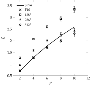
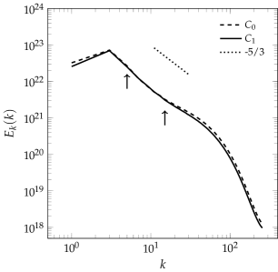
Figure 1: Left panel: structure function scaling exponent, $\zeta$, as a function of structure function order, $p$, for mesh resolutions of $128^{3}$, $256^{3}$, and $512^{3}$. The error bars indicate 95% confidence intervals for the exponent fits. The model by She & Leveque (1994) is provided for reference (black line). Additionally, the results from Federrath et al. (2010) are included for comparison. Our results show good agreement with Federrath et al. (2010), though both deviate from the She & Leveque (1994) prediction for high values of $p$. Right panel: the turbulent kinetic energy spectrum, $E_{k}(k)$, for solenoidally (dashed line) and compressively (solid line) driven turbulence. The dotted line gives the Kolmogorov -5/3 slope for reference, and the arrows indicate the limits of the inertial range. The spectra for both driving modes are very similar, and the inertial range slopes agree well with those obtained by Federrath et al. (2010) (see text).

for different model resolutions. The results indicate that the exponents converge as the resolution increases, and the exponents from our best-resolved $512^{3}$ model agree well with those obtained by Federrath et al. (2010). Also, the dependence of the scaling exponents on the structure function order obtained from our simulations is characterized by a shallower slope than predicted by the She & Leveque (1994) model. This is consistent with other studies of compressible turbulence (see, e.g., Fisher et al., 2008). As pointed out by Federrath et al. (2010), based on simulations obtained at still higher resolutions, simulations with a resolution of $512^{3}$ can be considered converged. This is because at this resolution numerical errors are smaller than the scale of the natural variance inherent to turbulent flows, and thus have a small effect on solution accuracy. Subsequently, we adopted a resolution of $512^{3}$ as the standard resolution in our simulations.

The time-averaged turbulent kinetic energy spectra obtained in simulations with solenoidal forcing (shown with a dashed line) and compressive forcing (shown with a solid line) are depicted in the right panel of Figure 1. The spectra display the characteristics typical of driven turbulence, with the energy injected on large scales ($1\leq k\leq 4$ in our models) with the energy cascading down to smaller scales. We calculated the inertial range slopes for the region $5\leq k\leq 15$, chosen to coincide with the inertial range used by Federrath et al. (2010). This gave values of the slope in the inertial range of -1.90 for solenoidal forcing, and -1.89 for compressive forcing. These indicate a steeper dependence than the canonical value of -5/3 for Kolmogorov turbulence (shown with a dotted line in the right panel of Figure 1). These exponents closely match the results reported by Federrath et al. (2010). We conclude that our trial computer experiments produce results that are in good agreement with the previously reported simulations.

2.2.2 Analysis of ignition conditions

In order for a parcel of degenerate matter to produce a self-sustained detonation, it must be characterized by the following conditions: (1) ignition times must be shorter than the local dynamical timescale (Fowler & Hoyle, 1964; Arnett, 1996), (2) the burning parcel must have a small curvature on average (sizable and of regular shape; Sharpe, 2001), and finally, (3) the ignition times must also be shorter than the local mixing timescale (we term this as longevity). Conditions (1) and (2) have been extensively discussed in the astrophysical literature (see, e.g., Dursi & Timmes, 2006; Seitenzahl et al., 2009; Dunkley et al., 2013), but we are not aware of any study specifically addressing the longevity of prospective detonation kernels, which would require sufficiently realistic hydrodynamic simulations. The model employed here offers such an opportunity, and having complete control of the flow conditions in our model, we are well-positioned to address this aspect in detail.

We developed a set of tools enabling analysis of the distribution of ignition times from the perspective of the production of self-sustained detonations. To this end, we identified and tracked regions of interest characterized by relatively short ignition times. At this point, we are not in a position to strictly define the longest ignition time required to produce a self-sustained detonation, as this time depends on several factors, as explained in the previous paragraph. The detonation kernel analysis was performed only after the system had reached a quasi-steady state, and was applied over sufficiently long periods of time, as described below.

Clustering analysis

To identify prospective detonation kernels, defined as contiguous regions with ignition times not exceeding a certain threshold value, $\tau_{\mathrm{ign,pdk}}$, we masked cells on the hydro mesh that satisfied this criterion. We then used a flood-filling algorithm (Levoy, 1981, and references therein) to composite (cluster) the masked cells into contiguous regions. Because flood-filling algorithms are typically implemented using a recursive procedure, special consideration had to be taken to prevent exhausting memory made available by the computer system to the application (stack overflow), as the data sets are relatively large. We also note that our use of the threshold ignition time in defining the spatial extent of the kernels implies that we expect that ignition will occur anywhere inside this region, and will result in a detonation (self-sustaining of detonations requires additional characterization beside the ignition time, as discussed previously). Naturally, it is expected that the ignition times will vary inside the kernel, possibly attaining values much shorter than the specified threshold. We omit such details of the kernel structure from our considerations, as our focus is the existence of the detonation kernels.

The clustering analysis was performed at a certain time, denoted $t_{\mathrm{i,pdk}}$ here, from which the evolution of the prospective kernels could be studied. In this work, we tracked their evolution using both Eulerian and Lagrangian fluid flow representations, as described below.

Longevity analysis

Our aim in this analysis step was to determine for how long the originally-identified prospective kernels existed in the course of the simulation. This information can be considered from the Eulerian as well as Lagrangian points of view, and we used both approaches in the present work.

In the first step of the Eulerian approach, every prospective kernel was assigned a unique identifier. This identifier was then used as the initial value of a new hydro variable (passive mass tracer), which was advected with the flow. Thus, we created a set of mass tracers uniquely representing material of prospective detonation kernels. As the simulation progressed, at selected times for $t>t_{\mathrm{i,pdk}}$, we repeated the clustering analysis and identified new prospective kernels. We term these newly-identified kernels. At this point of the analysis procedure, time-evolved information about the distribution of the original prospective detonation kernels as described by the mass tracers, as well as the information about the newly-identified kernels is available.

Next, we must find which original kernels contribute material to the newly-identified kernels. This step is necessary because, due to the Eulerian character of our scheme, and numerical mixing, intermediate values of mass tracers can be found in the material of the newly-identified kernels. However, these new kernels are expected to contain at least some material from the original kernels. Such material can be relatively easily identified by looking for cells that are filled with material from only one of the original kernels. Thus, at this point we limit the origin of material of the newly-identified kernels to only a subset of original kernels (in the limit, all the original kernels may contribute to one or more of the new kernels).

In the final step of the Eulerian approach, we consider mixed cells (those that contain various fractions of the original kernels). Here the cells that contain at least 90 per cent of the specific original cluster material are assigned to the surviving remnant of this particular original cluster. This concludes the process of (re)construction of the prospective kernels at the new time level.

In the Lagrangian approach, we seeded simulations with passive tracer particles. Every particle was assigned an identifier corresponding to its parent prospective detonation kernel. The sets of time slices of particle distributions were used to calculate time-based velocity autocorrelation functions, $\rho(t)$ (Tennekes & Lumley, 1972). The autocorrelation functions were calculated individually for each cluster. These functions provide information about the time coherence of prospective kernels from the perspective of hydrodynamic mixing. We chose not to account for the potentially changing ignition times (due to expansion or contraction of material) in the Lagrangian analysis, as it primarily serves to corroborate the results of the Eulerian analysis.

Analysis of the prospective detonation kernels was continued either for several $\tau_{\mathrm{ign,pdk}}$, as specified in the clustering step described above, or until all prospective kernels had been destroyed. We considered a prospective kernel destroyed when we could no longer find on the mesh any cells that contained pure material from the original kernel. The Lagrangian method was performed along with the Eulerian analysis, and both were terminated at the same time.

Compactness analysis

An additional important consideration in the context of the ignition of self-sustained detonations is the morphology of the prospective detonation kernels. Stable detonations require continuous fronts of sufficiently low curvature (Sharpe, 2001). For simplicity, assuming that a kernel is spherical in shape, the curvature of the kernel surface (which is associated with the detonation front) inversely scales with the kernel radius. This simplifying assumption is not satisfied in general in hydrodynamic simulations of reactive flows, and in particular in our models. For example, prospective kernels may have the appearance of extended 2D-like structures, which cannot be easily characterized as spheres or assigned a single curvature value. We may measure by how much each kernel’s morphology deviates from spherical by calculating the kernel volume filling factor, $f_{\mathrm{pdk}}$. The kernel’s volume filling factor is defined as the fraction of volume occupied by the kernel material inside a spherical shell with a given inner and outer radius. The shell is centred at the kernel’s centre of mass. A filling factor of less than 1 then indicates that the material is not spherically arranged for that range of radii.

For each kernel, we calculated the dependence of the filling factor on radius starting from the kernel’s centre of mass and ranging to the radius at which the filling factor was zero. The kernel compactness can be understood in terms of the dependence of the volume filling factor on the distance from the kernel’s centre. A compact kernel would be characterized by a relatively large filling factor at small radii. Then the requirement of low curvature of the detonation front, in our adopted simplified representation of spherical kernels, would be satisfied by compact kernels with appropriately large radii. Only such kernels may be considered as actual detonation kernels.

Fractal dimension estimation

An additional measure of a kernel’s morphology can be obtained by estimating the fractal dimension of its surface. The fractal dimension reflects on the object’s morphological complexity, and more specifically describes how a structure’s detail changes with scale. When a fractal analysis is applied to a kernel’s surface, it then characterizes how the amount of structure in the surface depends on scale. Therefore, the greater the fractal dimension of a kernel’s surface, the greater the complexity of its shape. In the work presented here, the kernel surface fractal dimension was estimated using a box-counting method (Falconer, 2003).

3 Results and Discussion

As mentioned in Section 1, the successful formation of a detonation in white dwarf material depends on several necessary conditions relating to the minimum sizes of ignition kernels, their morphology, and their corresponding ignition delay times. In this section, we systematically examine the likelihood of explosive nuclear burning for varying degrees of compressibility in the turbulent driving. For the simulations using different stirring models (characterized by a different degree of compressibility in the turbulent driving, $\zeta_{c}$), we perform a clustering procedure which identifies the material that has ignition times below a given threshold and produces a set of separate, contiguous regions. If the mass of the cluster exceeds the critical mass deemed necessary to produce a self-sustained detonation (see, e.g., Dursi & Timmes, 2006), we tentatively identify the cluster as an ignition kernel. This identification is only tentative as such kernels must satisfy additional criteria in order to produce self-sustained detonations. First, the kernel material must not mix with the surrounding medium for times shorter than the ignition time. That is, the kernels must survive for long enough for the detonation to fully develop. In addition, the ignition kernels should be compact. That is, they must be approximately spherically symmetric in order for a detonation to be uniformly powered by the burning zone.

3.1 Mass distribution of ignition times

Given that our initial conditions describe a region of fluid in a uniform state with no velocity, no kernels exist at the initial time. As turbulence is driven, the fluctuations in the hydrodynamic state appear and grow in amplitude. This causes variations in ignition times across the domain. Figure 2

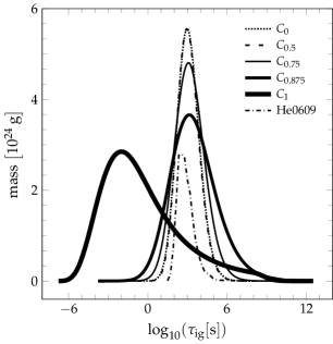
Figure 2: Mass distributions as a function of carbon ignition time for various values of $\zeta_{c}$. The distributions for the $C_{0}$ and $C_{0.5}$ models are visually indistinguishable. Increased compressibility in the drive causes the distributions to spread and develop more extended tails, indicating greater extremes in ignition times. Also shown is the mass distribution of helium ignition time calculated from a cube of boundary-layer data extracted from the He0609 model of Fenn et al. (2016) (dash-dotted line). This distribution displays an overall morphology consistent with the driven turbulence simulations.

shows the distribution of mass as a function of ignition time for our set of turbulence models. This form of the distribution is more natural for discussing the evolution of ignition times as the system parameters, such as the degree of compressibility in the driving, change. The distributions were obtained as time averages over 3 integral time scales. In the case of purely solenoidal and 50 per cent compressive driving, shown with dotted and dashed curves in Figure 2, respectively, the distributions are nearly identical, and cannot be distinguished in the figure. These distributions are nearly symmetric, with most mass residing near an average ignition time of approximately $1000\text{\,}\mathrm{s}$. They also have a relatively small dispersion, with no material present (an amount less than ${10}^{-3}$ of the peak mass) for ignition times shorter than about $1\text{\,}\mathrm{s}$. The mass distributions become progressively broader and asymmetric as the degree of compressibility in the driving increases. For example, the shortest ignition times observed in the $C_{0}.75$ and $C_{0}.875$ models are approximately $0.14\text{\,}\mathrm{s}$ and $8\text{\times}{10}^{-3}\text{\,}\mathrm{s}$. The distribution assumes a qualitatively different shape in the case of the fully compressively driven model $C_{1}$. In this case, the distribution is strongly asymmetric, with pronounced tails extending down to approximately $3\text{\times}{10}^{-7}\text{\,}\mathrm{s}$.

3.2 Spatial distribution of ignition times

Figure 3

Figure 3: Pseudocolour maps showing ignition times for the interior and exterior surfaces for the $C_{0}$, $C_{0}.875$, and $C_{1}$ models. Each volume shown here was created by replicating the original domain in the remaining octants of the Cartesian coordinate system whose origin lies at the corner of the original domain. Since our simulations use periodic boundary conditions, this results in continuous structures across the coordinate planes. The average colour in each model illustrates the extreme values of ignition times. Fluid structures also become increasingly distinct with increasing $\zeta_{c}$, as the prevalence of shocks increases.

shows pseudocolour maps (in log scale) of ignition times for the $C_{0}$, $C_{0}.75$ , and $C_{1}$ models, in the left, middle, and right panel, respectively. When plotting the ignition times, we use the same scale, which allows for making a qualitative comparison of spatial variations in ignition times between models. In particular, the $C_{0}$ model is characterized by the most uniform spatial distribution of ignition times, with clearly-visible small-scale structure. This picture is consistent with our analysis of the mass distributions as a function of ignition times discussed in Section 3.1. As the degree of compressibility in the drive increases, however, the spatial distribution of the ignition times becomes progressively more non-uniform. In the case of the purely compressively-driven model, $C_{1}$, there exist sharply-delineated regions of short and long ignition times, resulting in an overall patchy appearance of the distribution. This is due to the presence of shocks in strongly compressively-driven models. In such cases, the ignition time is relatively long in the region upstream of the shock, while it is the shortest immediately behind the shock.

The spatial distributions of ignition times can be formally characterized using spatial autocorrelation functions of ignition times. We found that in the models in which driving was not strongly compressive, the autocorrelation function provided evidence that ignition times typically varied in structures spanning 5-6 mesh cells. In contrast, the same analysis applied to the purely compressively-driven model formally indicated the presence of structures on scales below the mesh cell width. This result is consistent with the patchy appearance of the distribution of ignition times in this case, implying that the ignition times varied strongly on small scales (separating individual ‘patches’). We point out that integral scales comparable to or smaller than the mesh cell width either point to the presence of under-resolved physics effects or a failure of the analysis procedure. The presence of narrow regions occupied by strong gradients of ignition times reflects on the existence of shock fronts. In this case, the autocorrelation function no longer provides information about the integral scale of the flow, as the flow itself is no longer homogeneous, but composed of a collection of shocked gas regions that cool and rarefy before they are overrun by other shocks.

3.3 Existence of detonation kernels

As mentioned in Section 2.2.2, a detonation kernel that will produce a self-sustained detonation must be characterized by ignition times shorter than the local dynamical timescale, small curvature, and must be able to preserve its integrity for long enough for a detonation to fully develop. To this end, we applied the clustering analysis (cf. Section 2.2.2) to models $C_{0}$, $C_{0.875}$, and $C_{1}$, using ignition time thresholds, $\tau_{\mathrm{ign,pdk}}$, of ${10}^{-5}\text{\,}\mathrm{s}$, $1\text{\,}\mathrm{s}$, and $100\text{\,}\mathrm{s}$, respectively. These ignition time thresholds were selected in such a way that at least one prospective detonation kernel was produced (in the case of the $C_{0}$ and $C_{0.875}$ models), and in the case that many kernels were produced, they were spatially well-separated (in the case of the $C_{1}$ model). Furthermore, we disregarded any prospective kernels containing fewer than ${10}^{4}$ mesh cells, as we deemed such small kernels as computationally under-resolved.

Figure 4(a)

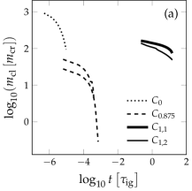
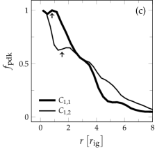
Figure 4: Left panel: Eulerian analysis showing cluster masses and lifetimes for the models $C_{0}$ (dotted line), $C_{0}.875$ (dashed line), and $C_{1}$ (solid lines). For the latter two models, the largest two observed clusters are shown. The $C_{0}$ model developed only one cluster. The clusters in the $C_{1}$ model are likely ignition candidates, and are differentiated by the subscripts 1 and 2. No other models have clusters likely to ignite. Tracking of each cluster ceased when no unmixed original cluster material remained. Middle panel: Lagrangian cluster analysis. Autocorrelations of Lagrangian tracer particles originating in each cluster. Final times appear different from the Eulerian analysis because the particles retained their identity and could be tracked indefinitely. This analysis shows cluster dissolution due to mixing. Integral timescales for each cluster obtained by integrating the autocorrelation functions agree well with the cluster lifetimes found in the Eulerian analysis. Right panel: Filling factors for clusters from the $C_{1}$ model. The clusters shown are the same depicted in the other panels. The horizontal axis is normalized to the minimum ignition kernel radius (calculated using the average cluster density), for each cluster. Values of 1 indicate that a sphere of the given radius centred at the cluster’s centre of mass is completely filled; values less than 1 indicate incomplete filling and departure from a spherical structure. The arrows indicate the minimum viable ignition kernel radius, calculated using the average density of the enclosed material, rather than the average cluster density. $C_{1,1}$ is completely filled at this radius, indicating it is a likely ignition candidate. $C_{1,2}$ is not, and thus is unlikely to produce a self-sustained detonation.

shows the time evolution, in units of the corresponding threshold ignition times, of the prospective detonation kernel mass. The kernel mass is shown in log scale, and is normalized to the critical mass. The critical mass is the mass of a spherical region with radius equal to the critical radius, $r_{\mathrm{ig}}$, as given by equation 11 of Dursi & Timmes (2006), with $\beta=0.77$ and for a carbon mass fraction of 0.5. In the calculation of the critical mass, we used the average kernel mass density.

In the case of the purely solenoidally-driven model $C_{0}$, only one cluster was found, and was destroyed very quickly after less than ${10}^{-5}$ ignition times. We found two clusters in the $C_{0.875}$ model, which again were relatively quickly destroyed after less than ${10}^{-3}$ ignition times. In contrast, the fully compressively-driven model $C_{1}$ produced two clusters that survived essentially untouched for more than 10 ignition times. It is worth pointing out that the initial mass of the cluster, expressed in terms of the critical mass, does not guarantee the survival of the cluster, as demonstrated in the $C_{0}$ model, in which case the initial kernel mass was approximately 1000 times the critical mass.

We computed approximate prospective detonation kernel decorrelation times by integrating the particle velocity autocorrelation functions for each kernel (cf. Section 2.2.2). Figure 4(b) shows the time evolution of these velocity autocorrelation functions. The typical thus-estimated decorrelation times were on the order of $2\text{\times}{10}^{-5}$, $3\text{\times}{10}^{-3}$, and 13 ignition times for kernels found in models $C_{0}$, $C_{0.875}$, and $C_{1}$, respectively. These Lagrangian analysis results closely follow and confirm the results of the Eulerian kernel longevity analysis.

Figure 4(c) shows the filling factor of prospective detonation kernels, $f_{\mathrm{pdk}}$, for the two kernels found in the fully compressively-driven model. In the figure, the radial dependence of the filling factor for $C_{1,1}$ and $C_{1,2}$ are shown with thick and thin solid lines, respectively. The radial coordinate is scaled by the critical ignition radius, $r_{\mathrm{ig}}$, as defined above, again using the average kernel density. In the figure, the vertical arrows show the ignition radii based on the actual density profile of the kernels. We note that these radii differ from the critical kernel ignition radii estimated based on the average kernel density, as described above. This is because the central densities of the kernels are different from the average kernel densities. Specifically, density in the central region of the $C_{1,1}$ kernel is higher than the kernel’s average density. In contrast, the central region of the $C_{1,2}$ kernel is less dense than this kernel’s material on average. More importantly, the central regions of the $C_{1,1}$ kernel up to twice the kernel ignition radius are purely composed of material under ignition conditions. Although we cannot exclude the possibility that the $C_{1,2}$ kernel will produce a self-sustained detonation, the likelihood of such an outcome is much greater in the case of the $C_{1,1}$ kernel.

It is interesting to note that the morphology of prospective detonation kernels appears dependent on the compressibility of the drive. Prospective kernels found in solenoidally-driven models are characterized by a fractal dimension of about 2.62, while the fractal dimension of prospective kernels found in purely compressively-driven simulations is about 2.46. In general, these large fractal dimensions are indicative of substantial structure of the kernels’ surfaces. Furthermore, compressively-driven models appear to produce more organized flow. This is consistent with our qualitative comparison of the flow morphology presented in Section 3.2 (cf. Figure 3).

3.4 Application to white dwarf mergers

To allow for direct comparison of results presented in this work to simulations of white dwarf mergers, one must estimate the degree of compressibility of turbulence present in the simulated boundary layers. Only after such a connection is established will we be in a position to identify additional factors of importance in Type Ia explosions from merging white dwarfs.

3.4.1 Relevance of the adopted model

To provide an estimate of the compressibility typical of boundary layers in white dwarf merger simulations, we extracted a cube of data from the region in which a detonation formed in the He0609 model of Fenn et al. (2016). This region is depicted in Figure 10 of Fenn et al. (2016). The extracted data cube was $256\text{\,}\mathrm{km}$ per side, which is a factor of 8 larger than the computational box used in the present work. We used the merger model obtained about $2\text{\,}\mathrm{s}$ prior to the formation of the detonation (for reference, the dynamical timescale of the material in the extracted region was about $1\text{\,}\mathrm{s}$).

Using the extracted data, we estimated the degree of compressibility with help of the following procedure. In the first step, we decomposed the velocity field into purely solenoidal and purely compressive components (Balsara, 1998). This analysis indicated that the kinetic energy stored in the compressive component amounted to $\approx 37$ per cent of the total kinetic energy. Next, we estimated the degree of compressibility in the driving in our merger model by comparing the just-obtained amount of the kinetic energy stored in the compressive mode to the corresponding amount found in the database of turbulent simulations obtained in this work for different degrees of compressibility, $\zeta_{c}$. We found that the degree of compressibility with which the turbulence is driven in the mergers is $\zeta_{c}\approx 0.97$. (A similar relation between the degree of compressibility in the drive and the amount of kinetic energy stored in the compressive component of the velocity field was obtained by Federrath et al. (2010) in the context of modeling turbulence in the interstellar medium.)

Although the drive is nearly purely-compressive in our He0609 model, it is not clear whether such a drive will efficiently produce detonation kernels. This is because of the strong dependence of prospective detonation kernel properties on the drive compressibility found in our simulations for $\zeta_{c}$ above 0.875. However, the He0609 model (Fenn et al., 2016) provides evidence for the formation of detonations. Furthermore, the average pressure between a carbon-oxygen mixture and pure helium, for the same density and temperature, differ by less than about 17 per cent. This indicates that the dynamics of the flow in the helium models should not be qualitatively different from that in the carbon-oxygen models.

We compared the dependence of the mass distribution on the ignition time in the He0609 model to our series of turbulent models. The corresponding mass distribution in the He0609 model is shown with a dot-dashed line in Figure 2. In the figure, and for clarity of presentation, the He0609 mass distribution has been normalized to the maximum of the $C_{1}$ distribution, shown with a thick solid line in Figure 2. The corresponding ignition times in the He0609 case were computed using the triple-alpha burning timescale (Khokhlov & Ergma, 1986). Even though the He0609 distribution appears substantially different from that of the $C_{1}$ model, the difference in appearance is chiefly due to the difference in the ignition times between helium and carbon-oxygen mixtures. Indeed, closer analysis of the distribution shapes reveals their qualitative similarity.

Table LABEL:t:distStats [ cap = Ignition time distribution statistics, caption = Skewness and kurtosis for the $C_{0.875}$, $C_{1}$, and merger boundary layer ignition time distributions , label = t:distStats, ]ccc model & skewness kurtosis $C_{0.875}$ 0.46 3.38 $C_{1}$ 0.89 3.52 He0609 1.29 6.97 provides information about the skewness and kurtosis for mass distributions for a subset of relevant turbulence models and the He0609 merger. It is interesting to note that the mass distribution in the merger model is more strongly skewed and has heavier tails than the mass distribution produced by the purely compressively-driven $C_{1}$ model. This provides additional evidence for the similarity of the flow found in the merger simulations to that obtained in simulations of driven turbulence, justifying our approach. It also offers evidence that successful detonations can be formed in systems that are not driven purely compressively. In summary, we conclude that the turbulence developing in white dwarf merger models has generic properties reflected in dedicated driven turbulence models. The chief difference between the two is the numerical mesh resolution.

3.4.2 Key control parameters besides turbulence

Thus, apart from the details of turbulence developing in the boundary layer of the merging white dwarf binary, the thermonuclear ignition time is the key remaining factor controlling the detonability of the mixture. In turn, the ignition time chiefly depends on parameters of the binary. Here the two important factors are the mass of the primary component (that controls the depth of the potential well, and thus the density and temperature of the accreted material), and the composition of the companion star (that controls the composition of the accreted material). The detonation kernels would exist provided that ignition times found in the short ignition time tail of the mass distribution are sufficiently short. This has important implications in regard to the parameters of merging white dwarf binaries. The simulation-based limit for detonability in binary white dwarf mergers–the total mass of the system must exceed (Dan et al., 2014)–was obtained based on simulations that did not resolve turbulence. Thus, this limit only considers the average background conditions rather than the actual conditions that would be obtained in simulations resolving turbulence. It is conceivable that if such a limit exists in nature, it would correspond to a lower total system mass, and could be established by performing merger simulations in which turbulence is sufficiently resolved.

3.4.3 Numerical effects

The presence of the long-lived, large, and compact kernel $C_{1,1}$ offers evidence that self-sustained detonations can be produced in the boundary layers of merging, carbon-oxygen white dwarfs, provided that the primary is sufficiently massive. This argument is additionally strengthened by the realization that our turbulence simulations represent only a relatively small region of the boundary layer. One may conservatively estimate, based on the typical linear span of the large-scale vortices found in our merger models (ca. $100\text{\,}\mathrm{km}$, Fenn et al., 2016), compared to the size of our computational box ($32\text{\,}\mathrm{km}$), that there will potentially be dozens of prospective detonation kernels inside a single vortex. In addition, merger simulations indicate the presence of several large vortices coexisting at any given time during the violent phase of the merger. Therefore, it is expected that the boundary layer will be densely populated with detonation kernels, making an explosion essentially inevitable. However, the viable detonation kernel $C_{1,1}$ has a radius of only about $250\text{\,}\mathrm{m}$–significantly smaller than the mesh resolution of any white dwarf merger simulations performed to date. The fact that no detonations are observed in carbon-oxygen boundary layers of systems with a total mass below can then be explained by mesh resolution inadequate to resolve turbulence in simulations of merging white dwarfs binaries.

3.5 Relation to the Khokhlov’s semi-analytic detonation model

Khokhlov (1991b) considered a scenario in which a detonation is created in the process of gradual strengthening of pre-existing flow perturbations by plasma self-heating due to thermonuclear burning. Because realistic multidimensional simulations were not computationally feasible at the time of his study, Khokhlov adapted a statistical formulation of Meyer & Oppenheim (1971) to describe distribution of plasma temperature fluctuations, or ignition times, on small scales. He studied the evolution of ignition time distributions due to thermonuclear self-heating, and concluded, in accordance with Meyer & Oppenheim (1971), that a fluid parcel (prospective detonation kernel) can produce a self-sustained detonation provided the energy release by individual parts of the parcel are synchronized in time.

Our model offers an improvement upon Khokhlov’s approach by considering a realistic turbulent flow field, including the effects due to the flow compressibility. We showed that in this case distributions of flow perturbations, and thus the distributions of the related ignition times, are no longer Gaussian, but become progressively more asymmetric as the degree of compressibility in the turbulent drive increases (cf. Figure 2 and Table LABEL:t:distStats). Also, compressibility qualitatively changes the flow structure with ignition kernels isolated by relatively large and smooth regions filled with expanding, shocked gas in the models with strongly compressible drive (cf. Section 3.2). Finally, time coherence of the ignition centres, postulated by Meyer & Oppenheim (1971) in order to produce strong ignitions, is no longer needed as individual kernels considered in our model are capable of producing self-sustained detonations.

Although we do not explicitly include self-heating due to thermonuclear burning in our model, we demonstrated that such models form a single family of solutions with models obtained at various times differing only by the average background temperatures. This implies that the mass distributions shown in Figure 2 would, on average, undergo a horizontal shift toward shorter ignition times as self-heating continues to increase the background temperature. This is qualitatively consistent with the predicted by Khokhlov evolution of ignition times (see Section 3.4 and Figure 6 in Khokhlov, 1991b).

3.6 Application to explosions of Chandrasekhar-mass white dwarfs

Here we consider the most popular SD scenario in which an explosion of a Chandrasekhar-mass white dwarf is initiated in the process of a deflagration. In the original model proposed by Nomoto and his collaborators (Nomoto et al., 1976, 1984), the ignition occurs in the centre of the white dwarf. Recent studies, however, indicate that the large scale convection present in the core region before the explosion may be responsible for advecting one or more nascent deflagrating bubbles $\approx 100$ km away from the white dwarf centre (Höflich & Stein, 2002; Nonaka et al., 2012). Due to buoyancy effects, the following evolution strongly depends on how asymmetric the initial conditions for the growth of the burning bubble are. If the ignition occurs sufficiently close to the centre, the burning region will grow and remain spherically-symmetric on average; otherwise, buoyancy forces will induce a large scale acceleration of the burning bubble (Niemeyer et al., 1996; Malone et al., 2014). In either case, the flame is subjected to a range of instabilities, with the Rayleigh-Taylor instability playing the dominant role in its large-scale evolution (Khokhlov, 1995; Zhang et al., 2007).

3.6.1 Delayed detonation

It is commonly accepted that as the flame reaches low-density (${\approx}10^{7}$ g cm^-3) outer layers of the white dwarf, it becomes susceptible to turbulence and fragments (Hillebrandt & Niemeyer, 2000; Bell et al., 2004). This particular phase of the flame evolution has been considered as a possible source of a DDT originally postulated by Khokhlov (1991a). Unfortunately, the flow near the flame region during that phase is subsonic (Röpke, 2007), and well-resolved computer models failed to produce conditions conducive to DDT (Zingale et al., 2005; Aspden et al., 2010, 2011; Woosley et al., 2011b). We cannot exclude a possibility that a low Mach number approximation (Bell et al., 2004) used in those dedicated, high-resolution simulations prevented capturing important effects related to the flow compressibility. But it is also possible that other physics components omitted from consideration in the present study, such as plasma magnetization and/or viscosity, act as additional reservoirs of energy that under certain conditions could be tapped into to initiate formation and support growth of the detonation kernels.

3.6.2 Gravitationally Confined Detonation (GCD)

GCD models follow the evolution of the deflagrating bubble after it is ignited slightly off-centre (Plewa et al., 2004; Seitenzahl et al., 2016), in accordance with models of dense cores of massive white dwarfs prior to the ignition (Nonaka et al., 2012, and references therein). Although shock-to-detonation transitions were observed in several model realizations after the bubble material converged and collided in a region opposite the breakout point (Plewa, 2007; Townsley et al., 2007), turbulence and strong acoustic perturbations coexist in GCD models also at earlier times. For example, a bow shock was observed forming ahead of the deflagrating bubble prior to its breakout. This shock sweeps through the surface layers, which very likely are turbulent due to the combined effects of rotation, shell burning, and accretion.

Significant amount of turbulence is generated when the bubble material moves over the surface, and mixes with and accelerates the outermost, fuel-rich layers. Although it is difficult to expect a detonation produced while the bubble ashes flow horizontally over the stellar surface due to relatively low densities, a strongly mixed, turbulent flow (see Jordan et al., 2012, for a qualitative analysis of turbulence generated during this phase) ultimately converges and collides inside a region opposite the breakout point.

Apart from a possibility of a detonation triggered directly by a shock, the plasma inside the convergence region is highly turbulent with significant amount of strong, acoustic perturbations. Although several 3D GCD models have been presented in the literature (Röpke et al., 2007; Jordan et al., 2008; Seitenzahl et al., 2016), meshes used in those simulations did not have resolution necessary to describe turbulence or resolve prospective detonation kernels.

3.6.3 Pulsating Reverse Detonation (PRD)

In the PRD scenario (Bravo et al., 2009, and references therein) a deflagration is ignited in one or more regions in the core. In contrast to GCD, however, the deflagrating material is contained inside the star and the released energy is spent on inducing (radial) pulsations of the white dwarf. After the initial expansion phase, the star contracts and an accretion shock forms at some distance above the stellar surface. This accretion shock eventually produces a converging detonation wave.

Some comments on relation between GCD and PRD models are due. Accretion shocks were observed in GCD models with relatively energetic deflagration phases (see, e.g. Y70YM25 and Y75YM50 models in Plewa, 2007). Those models were characterized by relatively stronger white dwarf expansion and slower surface flows, and therefore were less conducive to prompt shock-to-detonation transitions. The important difference is that the deflagrating bubbles in GCD retained their structural integrity during their ascent from the core region to the surface. It is not clear what physical mechanism could be responsible for destruction of bubbles in PRD, and numerical effects cannot be excluded.

Regardless qualitatively different outcome of the deflagration stage, the PRD models feature a strongly perturbed surface layer that is subjected to compression during the contraction phase. These are conditions in which we predict detonations kernels will form.

4 Summary

We have performed a series of simulations of compressible, driven turbulence under conditions representative of those found in the boundary layer in white dwarf mergers with heavy primaries. In the present study, these conditions correspond to a $0.8+$1.2\text{\,}\mathrm{\mathrm{M_{\odot}}}$$ carbon-oxygen binary with an average density of $4\text{\times}{10}^{6}\text{\,}\mathrm{g}\text{\,}{\mathrm{cm}}^{-3}$, temperature of $1\text{\times}{10}^{9}\text{\,}\mathrm{K}$, and a 50/50 carbon-oxygen composition.

We used a spectral forcing method to drive turbulence in a cubic domain, and studied the dependence of the likelihood of forming a self-sustained detonation on the degree of compressibility in the driving. We demonstrated the formal correctness of the procedure adopted to model turbulence, and simulations displayed characteristics (scaling of exponents of the velocity structure function, kinetic energy spectra) consistent with those obtained in similar studies of compressible turbulence.

We constructed mass distributions as a function of the mixture ignition time. We identified and tracked the evolution of prospective detonation kernels. We analysed these prospective kernels to quantify their longevity, mass, and morphology in the context of detonability. We also extracted data from the boundary layer region in a simulation of merging white dwarfs (He+C/O), and drew comparisons with our driven turbulence simulation results.

Our major findings and conclusions are summarized as follows:

1. [i]

2. Mass distributions as a function of ignition time indicate the presence of a heavy tail extending toward short ignition times, provided that the turbulence is driven compressively.

3. The analysis of the flow field of the ignition region extracted from the He0609 model of Fenn et al. (2016) shortly prior to helium ignition indicates that the turbulent drive does not need to be purely compressive in order to produce self-sustained detonations. The inferred degree of compressibility in the turbulent drive found in this model is about 97 per cent.

4. We demonstrated the overall similarity of the statistical properties of the mass distributions found in merger simulations and in our models. This justifies our approach to modeling the physics participating in the evolution of boundary layers in merging white dwarfs.

5. In our purely compressively-driven model, we found a substantial amount of material characterized by ignition times much shorter than the turbulent mixing timescale. Furthermore, we found this material organized in the form of centrally-condensed clusters. We identified these clusters as detonation kernels capable of producing self-sustained detonations.

6. The observed detonation kernel have a radius of about $250\text{\,}\mathrm{m}$, which is notably smaller than the spatial resolution of any 3D white dwarf merger simulations performed to date. We conclude that, in order to correctly account for important physics participating in the process of merging binary white dwarfs, computer simulations must resolve flow structures on scales on the order of $0.1\text{\,}\mathrm{km}$.

7. Our results indicate a high probability of detonations in the carbon-rich boundary layers of binary white dwarf systems with a total mass lower than previously advocated. In particular, the simulation-derived lower limit of the total white dwarf binary system mass of , as suggested by Dan et al. (2014), may require revision. Adequately resolved simulations will likely allow for detonations in systems of lower total mass, thus broadening the population of binary white dwarf systems capable of producing Type Ia supernova explosions.

8. The proposed detonation mechanism also applies to single degenerates, and we identified possible sites harboring turbulence and strong acoustic perturbations in all popular explosion models of Chandrasekhar-mass white dwarfs. In the context of DDT mechanism in the delayed detonation model, we advocate the need for performing DNS studies of thermonuclear deflagrations at low densities using fully compressible hydrocodes.

The results of our study suggest a number of possible future research directions. The average conditions adopted here correspond to conditions characteristic of the boundary layer of a relatively massive, $0.8+$1.2\text{\,}\mathrm{\mathrm{M_{\odot}}}$$, carbon-oxygen white dwarf binary. It would be important to consider conditions corresponding to systems with less massive carbon-oxygen primaries, and corroborate our conclusions in regard to the minimal value of the total system mass required for detonations. Simulations probing the parameter space of average density, temperature, and composition should be conducted. As we have recently shown (Fenn et al., 2016), self-heating from nuclear energy release has an important effect on simulation outcomes. Therefore, simulations of driven turbulence accounting for the effects due to nuclear burning should be performed in order to improve the conclusions drawn from the simplified model presented here.

References

- Arnett (1996) Arnett W. D., 1996, Supernovae and nucleosynthesis. An investigation of the history of matter, from the Big Bang to the present. Princeton University Press, Princeton
- Aspden et al. (2010) Aspden A. J., Bell J. B., Woosley S. E., 2010, ApJ, 710, 1654
- Aspden et al. (2011) Aspden A. J., Bell J. B., Woosley S. E., 2011, ApJ, 730, 144
- Balsara (1998) Balsara D. S., 1998, ApJS, 116, 133
- Bell et al. (2004) Bell J. B., Day M. S., Rendleman C. A., Woosley S. E., Zingale M. A., 2004, Journal of Computational Physics, 195, 677
- Blondin et al. (2013) Blondin S., Dessart L., Hillier D. J., Khokhlov A. M., 2013, MNRAS, 429, 2127
- Bravo & García-Senz (2006) Bravo E., García-Senz D., 2006, ApJ, 642, L157
- Bravo et al. (2009) Bravo E., García-Senz D., Cabezón R. M., Domínguez I., 2009, ApJ, 695, 1257
- Childs et al. (2012) Childs H., et al., 2012, in , High Performance Visualization–Enabling Extreme-Scale Scientific Insight. pp 357–372
- Colella & Woodward (1984) Colella P., Woodward P. R., 1984, J. Comput. Phys., 54, 174
- Dan et al. (2014) Dan M., Rosswog S., Brüggen M., Podsiadlowski P., 2014, MNRAS, 438, 14
- Davidson (2004) Davidson P. A., 2004, Turbulence : an introduction for scientists and engineers. Oxford University Press, Oxford, UK
- Dunkley et al. (2013) Dunkley S. D., Sharpe G. J., Falle S. A. E. G., 2013, MNRAS, 431, 3429
- Dursi & Timmes (2006) Dursi L. J., Timmes F. X., 2006, ApJ, 641, 1071
- Eswaran & Pope (1988) Eswaran V., Pope S. B., 1988, Computers and Fluids, 16, 257
- Falconer (2003) Falconer K. J., 2003, Fractal geometry : mathematical foundations and applications. J. Wiley & Sons, Chichester, New York
- Federrath et al. (2010) Federrath C., Roman-Duval J., Klessen R. S., Schmidt W., Mac Low M.-M., 2010, A&A, 512, A81
- Fenn et al. (2016) Fenn D., Plewa T., Gawryszczak A., 2016, MNRAS, 462, 2486
- Fisher et al. (2008) Fisher R. T., et al., 2008, IBM Journal of Research and Development, 52, 127
- Fowler & Hoyle (1964) Fowler W. A., Hoyle F., 1964, ApJS, 9, 201
- Fryxell et al. (2000) Fryxell B., et al., 2000, ApJS, 131, 273
- Gamezo et al. (2005) Gamezo V. N., Khokhlov A. M., Oran E. S., 2005, ApJ, 623, 337
- Guillochon et al. (2010) Guillochon J., Dan M., Ramirez-Ruiz E., Rosswog S., 2010, ApJ, 709, L64
- Hillebrandt & Niemeyer (2000) Hillebrandt W., Niemeyer J. C., 2000, ARA&A, 38, 191
- Höflich & Stein (2002) Höflich P., Stein J., 2002, ApJ, 568, 779
- Hoyle & Fowler (1960) Hoyle F., Fowler W. A., 1960, ApJ, 132, 565
- Jordan et al. (2008) Jordan IV G. C., Fisher R. T., Townsley D. M., Calder A. C., Graziani C., Asida S., Lamb D. Q., Truran J. W., 2008, ApJ, 681, 1448
- Jordan et al. (2012) Jordan IV G. C., et al., 2012, ApJ, 759, 53
- Kashyap et al. (2015) Kashyap R., Fisher R., García-Berro E., Aznar-Siguán G., Ji S., Lorén-Aguilar P., 2015, ApJ, 800, L7
- Khokhlov (1991a) Khokhlov A. M., 1991a, A&A, 245, 114
- Khokhlov (1991b) Khokhlov A. M., 1991b, A&A, 246, 383
- Khokhlov (1995) Khokhlov A. M., 1995, ApJ, 449, 695
- Khokhlov & Ergma (1986) Khokhlov A. M., Ergma E. V., 1986, Soviet Astronomy Letters, 12, 152
- Khokhlov et al. (1997) Khokhlov A. M., Oran E. S., Wheeler J. C., 1997, ApJ, 478, 678
- Levoy (1981) Levoy M., 1981, in SIGGRAPH ’81. pp 6–12
- Malone et al. (2014) Malone C. M., Nonaka A., Woosley S. E., Almgren A. S., Bell J. B., Dong S., Zingale M., 2014, ApJ, 782, 11
- Meyer & Oppenheim (1971) Meyer J. W., Oppenheim A. K., 1971, Combust. Flame, 17, 65
- Mochkovitch & Livio (1989) Mochkovitch R., Livio M., 1989, A&A, 209, 111
- Moll et al. (2014) Moll R., Raskin C., Kasen D., Woosley S. E., 2014, ApJ, 785, 105
- Niemeyer et al. (1996) Niemeyer J. C., Hillebrandt W., Woosley S. E., 1996, ApJ, 471, 903
- Nomoto et al. (1976) Nomoto K., Sugimoto D., Neo S., 1976, Ap&SS, 39, L37
- Nomoto et al. (1984) Nomoto K., Thielemann F.-K., Yokoi K., 1984, ApJ, 286, 644
- Nonaka et al. (2012) Nonaka A., Aspden A. J., Zingale M., Almgren A. S., Bell J. B., Woosley S. E., 2012, ApJ, 745, 73
- Oran & Gamezo (2007) Oran E. S., Gamezo V. N., 2007, Combustion and Flame, 148, 4
- Pakmor et al. (2010) Pakmor R., Kromer M., Röpke F. K., Sim S. A., Ruiter A. J., Hillebrandt W., 2010, Nature, 463, 61
- Plewa (2007) Plewa T., 2007, ApJ, 657, 942
- Plewa et al. (2004) Plewa T., Calder A. C., Lamb D. Q., 2004, ApJ, 612, L37
- Poludnenko et al. (2011) Poludnenko A. Y., Gardiner T. A., Oran E. S., 2011, Physical Review Letters, 107, 054501
- Raskin et al. (2014) Raskin C., Kasen D., Moll R., Schwab J., Woosley S., 2014, ApJ, 788, 75
- Röpke (2007) Röpke F. K., 2007, ApJ, 668, 1103
- Röpke et al. (2007) Röpke F. K., Woosley S. E., Hillebrandt W., 2007, ApJ, 660, 1344
- Seitenzahl et al. (2009) Seitenzahl I. R., Meakin C. A., Townsley D. M., Lamb D. Q., Truran J. W., 2009, ApJ, 696, 515
- Seitenzahl et al. (2016) Seitenzahl I. R., et al., 2016, A&A, 592, A57
- Sharpe (2001) Sharpe G. J., 2001, MNRAS, 322, 614
- She & Leveque (1994) She Z.-S., Leveque E., 1994, Physical Review Letters, 72, 336
- Tennekes & Lumley (1972) Tennekes H., Lumley J. L., 1972, First Course in Turbulence. MIT Press, Cambridge
- Timmes & Swesty (2000) Timmes F. X., Swesty F. D., 2000, ApJS, 126, 501
- Townsley et al. (2007) Townsley D. M., Calder A. C., Asida S. M., Seitenzahl I. R., Peng F., Vladimirova N., Lamb D. Q., Truran J. W., 2007, ApJ, 668, 1118
- Woosley et al. (2011a) Woosley S. E., Kerstein A. R., Aspden A. J., 2011a, ApJ, 734, 37
- Woosley et al. (2011b) Woosley S. E., Kerstein A. R., Aspden A. J., 2011b, ApJ, 734, 37
- Yungelson & Kuranov (2017) Yungelson L. R., Kuranov A. G., 2017, MNRAS, 464, 1607
- Zel’dovich et al. (1970) Zel’dovich Y. B., Librovich V. B., Makhviladze G. M., Sivashinskil G. I., 1970, Journal of Applied Mechanics and Technical Physics, 11, 264
- Zhang et al. (2007) Zhang J., Messer O. E. B., Khokhlov A. M., Plewa T., 2007, ApJ, 656, 347
- Zingale et al. (2005) Zingale M., Woosley S. E., Rendleman C. A., Day M. S., Bell J. B., 2005, ApJ, 632, 1021