The Nature of Turbulence in the LITTLE THINGS Dwarf Irregular Galaxies

Abstract

We present probability density functions and higher order (skewness and kurtosis) analyses of the galaxy-wide and spatially-resolved H i column density distributions in the LITTLE THINGS sample of dwarf irregular galaxies. This analysis follows that of Burkhart et al. (2010) for the Small Magellanic Cloud. About 60% of our sample have galaxy-wide values of kurtosis that are similar to that found for the Small Magellanic Cloud, with a range up to much higher values, and kurtosis increases with integrated star formation rate. Kurtosis and skewness were calculated for radial annuli and for a grid of 32 pixel $\times$ 32 pixel kernels across each galaxy. For most galaxies, kurtosis correlates with skewness. For about half of the galaxies, there is a trend of increasing kurtosis with radius. The range of kurtosis and skewness values is modeled by small variations in the Mach number close to the sonic limit and by conversion of H i to molecules at high column density. The maximum H i column densities decrease with increasing radius in a way that suggests molecules are forming in the weak field limit, where $H_{2}$ formation balances photodissociation in optically thin gas at the edges of clouds.

1 Introduction

Turbulence in the interstellar medium (ISM) has been proposed to be a key element in determining the star formation laws of galaxies, especially in low gas density regimes such as those observed in the outer disks of spirals and in dwarf irregular (dIrr) galaxies. Turbulent motions can both hinder star formation (SF) by preventing the collapse of star-forming clouds (e.g. Mac Low & Klessen, 2004) and help it by collecting gas into dense regions (Elmegreen, 1993, 2002). There is also an expected relation between star formation activity and turbulence in the form of increased velocity dispersions due to the injection of energy from stars via stellar winds and, especially, supernovae explosions (SNe) (e.g. Mac Low & Klessen, 2004; Tamburro et al., 2009). However, it is thought that SF cannot be the only driver of turbulence in the ISM, as observed velocity dispersions remain approximately constant across the disk, even in low density and low star-formation regions in both spirals (Tamburro et al., 2009) and dwarfs (Hunter et al., 1999, 2001).

Previous studies of turbulence in the ISM in dwarf galaxies have focused largely on determining the source of the turbulence. Stilp et al. (2013), for example, measured turbulence in the atomic hydrogen (H i) of dwarf galaxies in the VLA-ANGST (Ott et al., 2012) and THINGS (Walter et al., 2008) surveys. They measured the velocity dispersions from stacked and averaged individual line-of-sight H i spectral profiles, either from the same radial annuli or from regions with the same SF surface density. They found that the measured velocity dispersions from regional “superprofiles” correlate best with baryonic and H i surface mass densities, indicating that some kind of gravitational instabilities are the most likely driving source. However, they found that none of the mechanisms they studied (which also included SF, magneto-rotational instability, and accretion-driven turbulence) could individually cause the observed level of turbulence in low SFR regions.

Dutta et al. (2009) used power spectra of the H i in a sample of seven dwarf galaxies (and one spiral) to look at turbulence in the ISM. They found a correlation between higher SFR per unit area and steeper power-law slopes for four of their sample, but caution that confirmation with a larger sample of galaxies was needed. Zhang et al. (2012) used Fourier transform spatial power spectra of velocity slices of varying widths to examine the turbulence in the ISM of a sample of LITTLE THINGS dwarf galaxies (Local Irregulars That Trace Luminosity Extremes, The H i Nearby Galaxy Survey, Hunter et al., 2012). Observed power-law slopes in H i-line intensity power spectra in the Milky Way (Crovisier & Dickey, 1983; Green, 1993; Dickey et al., 2001; Khalil et al., 2006) and Magellanic Clouds (Stanimirović & Lazarian, 2001; Elmegreen et al., 2001) are thought to be due to the presence of turbulence in the ISM (Zhang et al., 2012). The power-law behavior arises as driving sources input energy on large scales and the energy “cascades” down with little dissipation to small scales, where it dissipates (this assumes a nonmagnetic incompressible medium) (Kolmogorov, 1941). The range of scales where little dissipation occurs is known as the “inertial-range.” Hydrodynamic galaxy simulations by Bournaud et al. (2010), Pilkington et al. (2011), Combes et al. (2012), Hopkins et al. (2012), and Walker et al. (2014) show that large scale turbulence can be driven by gravitational instabilities, but that to maintain small-scale structures (clouds) in the ISM there needs to be a different source of energy — this is thought to be from SNe. Zhang et al. (2012) find no correlation between the inertial-scale spectral indices and star-formation rates (SFR), so conclude that non-stellar sources are required to provide turbulence in the inertial range, or that turbulent structures are not related to driving sources.

The relative importance of SNe and self-gravity for the generation of interstellar turbulence is not so clear in recent numerical simulations. While Ibanez-Mejia, et al. (2016) state that self-gravity is needed to explain the observed correlations between molecular cloud line-widths, sizes, and column densities (Heyer et al., 2009), Padoan et al. (2016) suggest that these correlations and others can result entirely from supernova pumping without self-gravity. Kim, Ostriker, & Kim (2014) and Kim & Ostriker (2015) also find that star formation properties, scale heights, and velocity dispersions in galaxies can be explained by supernova feedback. Still, internal cloud feedback from pre-main sequence winds is probably not generating the observed cloud line-widths, even though there is enough energy and momentum in the winds to do this; self-gravity seems to be involved instead (Drabek-Maunder et al., 2016). Li & Burkert (2017) and Li (2017) also note that self-gravitational energy generation dominates turbulent energy decay in local molecular clouds. Most likely, a combination of supernova energy and gravitational energy drive most interstellar turbulence, with self-gravity dominating on galactic scales and in cloud interiors, and supernovae dominating on intermediate scales, i.e., smaller than the disk thickness and particularly in the lower density gas. Magnetic field instabilities should also contribute to turbulence in the lower density gas (e.g., Piontek & Ostriker, 2007).

By examining the change of slopes in power-spectra from different velocity widths, Zhang et al. (2012) also confirm the work of Lazarian & Pogosyan (2000) that shows that H i power spectra made with different velocity width data trace different temperature phases of a multi-phase ISM. This means that observationally determining turbulent velocity spectral indices is complex and needs to be informed by models that include the multi-phase nature of the ISM. A multi-phase ISM consists of both a warm neutral medium (WNM) which is transonic, and a cold neutral medium (CNM) which is supersonic; so, unlike with the Kolmogorov nonmagnetic incompressible medium mentioned above, the ISM is compressible with both self-gravity and magnetic fields likely affecting turbulence. Higher sonic and Alfven Mach numbers indicate weaker magnetic fields and stronger shocks in the ISM. It has been suggested by Krumholz & McKee (2005) that the star formation rate (SFR) is at least partly determined by the sonic Mach number in the ISM.

Numerical simulations by Kraljic et al. (2014) suggest that the change in slope of the Schmidt-Kennicutt relation between gas surface density and SFR from the low gas density regime to high gas density regime is the result of a transition from subsonic to supersonic turbulence (see also Renaud et al., 2012). This transition may also be coupled to the transition from inefficient to efficient star formation. Dwarf irregular galaxies and the outer disks of spirals that are largely in the low gas surface density regime are, in this model, expected to have turbulence that is primarily subsonic as well as low efficiency star formation. Furthermore, in these low gas density regimes turbulence may be a very important process for bringing gas together into star-forming clouds since other processes believed to be crucial in high density gas environments do not work at low gas densities (e.g. Elmegreen & Hunter, 2006).

In this study we present an examination of the nature of the turbulence in the H i gas of a sample of nearby dIrr galaxies. (See Maier et al. 2016 for a companion study of spiral galaxies). In addition to constructing probability density functions (PDFs) of the integrated H i column densities, $N_{HI}$, we determine the third and fourth moments (skewness and kurtosis) of PDFs for comparison to models (Kowal et al., 2007, see also Konstandin et al. 2012). Skewness is a measure of the symmetry of the PDF distribution, and kurtosis is a measure of the sharpness of the peak and extent of the tails of the distribution. The analysis of higher order moments of $N_{HI}$ distributions follows the study of Burkhart et al. (2010) in which they determined the skewness and kurtosis values of the H i PDFs of the Small Magellanic Cloud (SMC) and inferred the Mach number of the gas from simulations. Burkhart et al. (2010) found that the turbulence in the SMC is transonic, which implies that the ISM is only weakly structured by turbulence compression.

The sample of dwarf irregulars used here is described briefly in Section 2. We present simple PDFs, the number of pixels as a function of integrated H i column density, as a function of radius in Section 3.1. For the skewness and kurtosis analysis that follows, we discuss galaxy-wide values and evidence for conversion of H i to molecules in Section 3.2.1, variations with radius from measurements in annuli in Section 3.2.2, and two-dimensional maps of values in Section 3.2.3. In Section 4 we present models that reproduce the skewness and kurtosis values that we find in terms of the Mach number of the gas and an upper limit to the HI column density. A summary is in Section 5.

2 Sample and Data

The sample of galaxies is taken from LITTLE THINGS (Hunter et al., 2012). This is a multi-wavelength survey of 37 dIrr galaxies and 4 Blue Compact Dwarfs (BCDs; Haro 29, Haro 36, Mrk 178, VIIZw 403), which builds on the THINGS project, whose emphasis was on nearby spirals (Walter et al., 2008). The LITTLE THINGS sample contains dwarf galaxies that are relatively nearby ($\leq$10.3 Mpc; 6″ is $\leq$300 pc), that contain gas, the fuel for star formation, and that cover a large range in dwarf galactic properties. The data used here include H i-line maps obtained with the Karl G. Jansky Very Large Array (VLA). The H i maps are characterized by high sensitivity ($\leq 1.1$ Jy beam^-1 per channel), high spectral resolution ($\leq$2.6 km s^-1), and high angular resolution ($\sim$6″). In addition we use 1516 Å FUV images obtained with the Galaxy Evolution Explorer satellite (GALEX; Martin et al., 2005) as a tracer of star formation over the past 100–200 Myrs. The galaxies and a few key parameters are listed in Table 1.

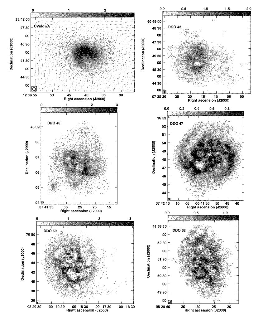
Figure 1: Robust-weighted integrated H i (moment 0) column density maps of the LITTLE THINGS dwarf irregular galaxies. See Hunter et al. (2012) for details. The maps are in units of $10^{21}$ atoms cm^-2, except for some galaxies where the units are $10^{18}$ atoms cm^-2 (DDO 87, DDO 101, F564-V3, LGS3, M81dwA, SagDIG).

In this study we use the robust-weighted integrated H i (moment 0) maps, shown in Figure 1. This gives us high angular resolution and is motivated by the 30-pc spatial resolution of the SMC used by Burkhart et al. (2010) that we wish to compare to. However, only 4 galaxies (DDO 69, IC 10, IC 1613, WLM) have high enough angular resolution to allow a 30-pc spatial resolution. In order to determine the effect of spatial resolution on the skewness and kurtosis values, we computed these values at 4 different spatial resolutions: the original angular resolution of the observations and maps smoothed, where possible, to 30 pc, 100 pc, and 200 pc beam-sizes. The original beam sizes are given in Table 2. A discussion of the effect of the varying resolutions on the results is presented below.

3 Analysis

The PDF of H i column density gives information about the range of $N_{HI}$ variations and the limiting values. The range is related to the ISM phase structure, which includes cool clouds and a warm intercloud medium, and it is related to substructure from self-gravity, pressure-swept shells, and compressive turbulence. The limiting values extend from the threshold of detection at low column density, which might coincide with lines of sight through purely warm-phase gas, up to either cool H i clouds or the transition to molecules. Here we study the $N_{HI}$ PDF for each galaxy in four radial bins, and for radii inside and outside the break radius of the exponential disks. We also determine the 3rd and 4th moments of the PDFs for whole galaxies, as functions of radius, and in square sub-region kernels. The results give some insight into the transition from atomic hydrogen to molecules, and they indicate an approximate way to determine the Mach number of the turbulence.

3.1 Simple PDFs as a function of radius

From the integrated H i maps with the original beam-sizes given in Table 2, we computed the number of pixels as a function of column density, $N_{HI}$. Pixels with $N_{HI}$ $\leq 15\times 10^{18}$ cm^-2, which represents several times the typical rms noise in the outskirts of the LITTLE THINGS galaxies, were eliminated from each galaxy in order to ensure good S/N. The pixel size is 1.5″ for all galaxies except for DDO 216 and SagDIG, which have 3.5″ pixels. In order to remove the overall decline of $N_{HI}$ with radius, which would otherwise dominate the PDF profile, we normalized the individual values with the average determined radially every $V$-band disk scale length, $R_{D}$. Before making the average $N_{HI}$ profiles, we clipped the integrated H i maps to remove pixels with values $\leq 15\times 10^{18}$ cm^-2, and only non-blank pixels were included. To find the radius of a given pixel in the plane of the galaxy, we used the galactic center, inclination, and position angle of the major axis determined from H i kinematic fits (Oh et al., 2015), where available, or from the optical $V$-band morphology (Hunter & Elmegreen, 2006), otherwise.

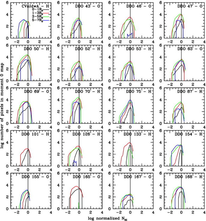
Figure 2: $N_{HI}$ PDFs as a function of distance from the center of the galaxy in units of disk scale length $R_{D}$. Wherever H i kinematic fits to the velocity field are available (Oh et al., 2015), parameters from those fits – galaxy center, inclination angle, major axis position angle – are used. Those galaxies are marked with an “H” for “H i” after the galaxy name. The rest of the galaxies used determinations from $V$-band morphologies (Hunter & Elmegreen, 2006) and are denoted “O” for “optical.” Pixels with $N_{HI}$ $\leq 15\times 10^{18}$ cm^-2 were eliminated to ensure good S/N.

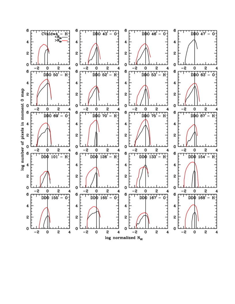
Figure 3: $N_{HI}$ PDFs before and after breaks in the galaxy’s $V$-band surface brightness profiles, $R_{Br}$, as given by Herrmann et al. (2013). DDO 47 and DDO 210 do not exhibit breaks in their exponential surface brightness profiles, so galaxy-wide PDFs are shown instead. Wherever H i kinematic fits to the velocity field are available (Oh et al., 2015), parameters from those fits – galaxy center, inclination angle, major axis position angle – are used. Those galaxies are marked with an “H” for “H i” after the galaxy name. The rest of the galaxies used determinations from $V$-band morphologies (Hunter & Elmegreen, 2006) and are denoted “O” for “optical.” Pixels with $N_{HI}$ $\leq 15\times 10^{18}$ cm^-2 were eliminated to ensure good S/N.

Figure 2 shows the PDFs of normalized $N_{HI}$  for each galaxy in 4 different radii bins: 0-1$R_{D}$, 1-3$R_{D}$, 3-5$R_{D}$, and 5-7$R_{D}$. The $R_{D}$ were determined by Herrmann et al. (2013) and are given in Table 1. Figure 3 shows the PDFs interior and exterior to the break, $R_{Br}$, in the $V$-band surface brightness profile, if one is present. The break marks a change in slope in the profile, with most bending downward and the exponential fall-off becoming steeper (Type II breaks), but a few bending upward and becoming shallower with radius (Type III). The $R_{Br}$ were measured by Herrmann et al. (2013) and are also given in Table 1.

Some of the PDF shapes in Figure 2 are Gaussian in the central regions (which means parabolic in these log-log plots) but they have sharper than Gaussian drop-offs at low and high $N_{HI}$. The PDFs are similar in shape to those made (not shown) without the cut-off of $N_{HI}$ below $15\times 10^{18}$ cm^-2, so the lack of tails in the PDFs of Figure 2 is not due to this cut-off. Patra et al. (2013) also saw a sharp drop off to higher $N_{HI}$ in PDFs of the FIGGS sample of dwarf galaxies. However, another common PDF shape in our sample is one in which the fall-off to lower normalized $N_{HI}$ is more gradual than to higher values, so the PDF is not symmetrical on a log-log plot.

For radial trends in the PDFs, for many of the galaxies we see that the PDFs are similar at different radii within a galaxy. This similarity for normalized $N_{HI}$ implies that the absolute $N_{HI}$ distribution does not extend up to some fixed value such as a fixed molecular transition threshold (e.g., Bigiel et al., 2008) or fixed dust opacity. The upper limit to the normalized column density, $N(HI)_{\rm max}$, is around a factor of 10 times the average in most of these cases, which is much less than the expected upper limit to the gas column density in general, especially since there is star formation. That the upper limit to the density is lower than expected, however, is not due to a larger beam-size since some of these galaxies have the highest linear resolution in our sample, as low as a 20 pc beam-size. This upper limit seems instead to imply that the disappearance of H i emission at high density, which is presumably from a transition to opaque H i or molecules, occurs at a relative value of column density, and is possibly driven by pressure and starlight. Although many of the galaxies have PDFs that are similar at different radii within the galaxy, other galaxies in Figure 2 have upper limits to the PDF functions that increase regularly with increasing annulus. This is partly because of the rejected pixels mentioned above; these cases have a more constant value of the maximum column density in absolute terms.

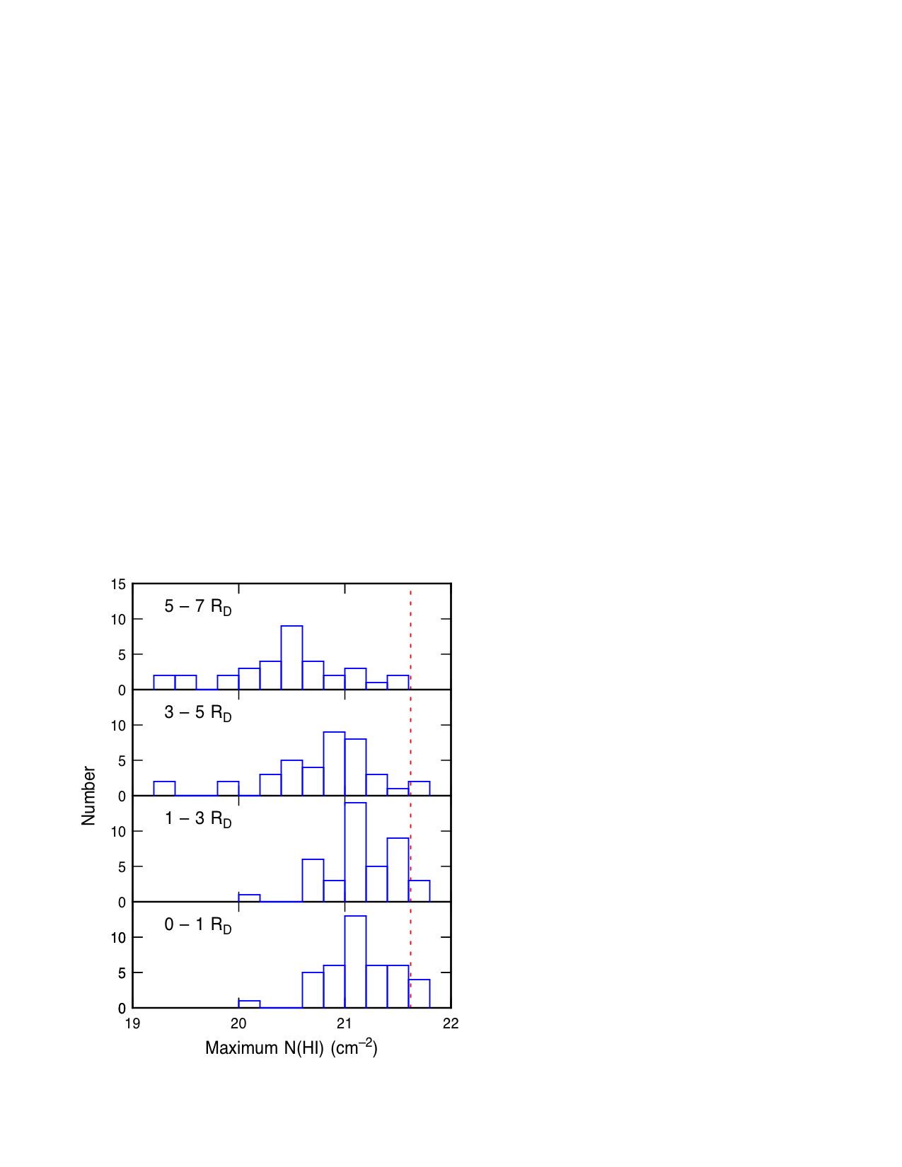
Figure 4: Histograms of the maximum value of $N_{HI}$ in four radial intervals for all of the galaxies in this survey. The vertical dashed line is the H i column density where the opacity to FUV radiation is unity at a metallicity of 1/8 solar, which is typical for these dIrrs. Most values of maximum $N_{HI}$ are much less than this opacity limit, which suggests that molecule formation is in the weak field limit, occurring where the H₂ formation rate at a cloud surface balances the photo dissociation rate.

Figure 4 shows histograms of the absolute maximum values of $N_{HI}$ for all galaxies in the four radial bins. The distributions of $N_{HI}$ shift toward lower values with increasing radius, and never exceed a maximum value (for our spatial resolution) of $\log N(HI)\sim 21.8$. These trends and maximum values give insight into the undetected high-density phases of the interstellar medium.

Molecule formation requires shielding of the molecules from background FUV radiation, and this shielding results from a combination of dust extinction and line absorption by similar molecules in the cloud envelopes (Krumholz et al., 2009; Bialy et al., 2016). According to Bialy et al. (2016), the total column density of H i through a slab that turns molecular with increasing depth depends only on the parameter $\alpha G$, which, for $H_{2}$ formation on dust grains, is given by their equation (22),

$$\alpha G=0.59I_{\rm FUV}\left({{100\;{\rm cm}^{-3}}\over{n_{\rm cloud}}}\right)\left({{9.9}\over{1+8.9{\tilde{\sigma}_{g}}}}\right)^{0.37}.$$ (1)

Here, $\alpha$ is the ratio of the H₂ photodissociation rate in free space to the H₂ formation rate, $G$ is the ratio of the dust to gas absorption cross sections times the maximum bandwidth in Hz for H₂ absorption in the Lyman-Werner bands, $I_{\rm FUV}$ is the local radiation field in units of the value in the solar neighborhood (Draine, 1978), $n_{\rm cloud}$ is the cloud density, and $\tilde{\sigma}_{g}$ is the normalized metallicity-dependent dust absorption cross-section per hydrogen nucleon. The product $\alpha G$ is the ratio of the shielded photo-dissociation rate to the H₂ formation rate. When $\alpha G$ is small, the H i layer at the edge of a cloud is limited by molecular self-absorption and photo-dissociation; when $\alpha G$ is large, dust opacity determines the H i column density at the cloud edge; $\alpha G=1$ represents the borderline between dust and dissociation attenuation for incoming radiation in the H i layer around an H₂ cloud.

For the dIrrs in our sample, the average metallicity is $Z^{\prime}\sim 1/8$ relative to solar, so the non-normalized dust absorption cross-section per hydrogen nucleon is $\sigma_{\rm g}\sim 1.9\times 10^{-21}Z^{\prime}\sim 2.4\times 10^{-22}$ cm^-2. The dust opacity in an H i cloud, $\sigma_{\rm g}N(HI)$, equals 1 when $N(HI)$ is the inverse of $\sigma_{\rm g}$, or $4.2\times 10^{21}$ cm^-2, which corresponds to $42\;M_{\odot}$ pc^-2 including He and heavy elements. This column density for opaque gas is much higher than our average $N_{HI}$, and close to the upper limit to $N_{HI}$ in the inner regions. Figure 4 has a dotted red line at this value, which is $\log N(HI)=21.62$. The histograms reach this value only in the inner parts of the galaxies. Thus, most of the local H i peaks in the main parts and outer disks of our galaxies are not optically thick from dust even though there is star formation at these radii. This implies that much of the H₂ gas associated with star formation, perhaps all but the molecules that are deeply embedded in dense self-gravitating cores, is self-shielded rather than dust-shielded. Then $\alpha G$ is small and $\sigma_{\rm g}N(HI)\sim\alpha G$ (from Eq. 19 in the limit of small $\alpha G$ in Bialy et al., 2016, considering that $N(HI)$ in that equation is for half of the cloud) for $N(HI)$ at the threshold of molecule formation. Small $\alpha G$ is also likely for our galaxies because $I_{\rm FUV}$ in equation (1) is small; these are low surface brightness galaxies with star formation surface densities that are lower than that in the solar neighborhood by a factor of 10 to 100.

Thus, molecule formation in our sample of dIrrs is mostly in the weak-field limit (Bialy et al., 2016), where the shielding column around a cloud is given by a balance between the integrated $H_{2}$ formation rate and the integrated $H_{2}$ destruction rate in the incident radiation field. Then $N(HI)_{\rm max}n_{\rm cloud}\propto I_{\rm FUV}$ and dust is relatively unimportant. Since $I_{\rm FUV}$ varies with radius, as well as from galaxy to galaxy, this is presumably why the peak $N_{HI}$ is not a fixed absolute value for different annuli in Figure 2.

We previously determined the average radial variations of $N(HI)$ and $I_{\rm FUV}$ for 20 LITTLE THINGS dIrrs to be $\propto\exp(-\xi r/R_{\rm D})$ for relative scale length $\xi=0.45\pm 0.32$ and $0.98\pm 0.80$, respectively, where $R_{\rm D}$ is the $V$-band disk scale length (Elmegreen & Hunter, 2015). The FUV intensity comes from the ratio of the volume emissivity to the opacity, which is the same as the ratio of the surface brightness of FUV to the surface density of gas. If the peak $N_{HI}$ is proportional to the average $<N(HI)>$, as suggested for many of the galaxies by Figure 2, then the average $H_{2}$ cloud density in the shielding envelope varies with galactocentric radius as the ratio of $I_{\rm FUV}$ to $<N(HI)>$, which is $n_{\rm cloud}\propto\exp(-\xi_{\rm cloud}r/R_{\rm D})$ for $\xi_{\rm cloud}=0.53\pm 1.07$ (Elmegreen & Hunter, 2015). We can compare this density variation to the expected pressure variation considering that the average pressure scales with the square of the column density, which for these gas-dominated and H i-dominated regions, is just $N(HI)$. Thus, the ISM pressure falls with radius as $P_{\rm ISM}\propto N(HI)^{2}\propto\exp(-[0.9\pm 0.64]r/R_{\rm D})$. This pressure variation is similar to that of the product of the $H_{2}$ transition cloud density and the square of the H i velocity dispersion (for which $\xi_{\rm disp}=0.10\pm 0.10$), which is $P_{\rm cloud}=\exp(-[0.73\pm 1.5]r/R_{\rm D})$. It follows that the envelopes of the clouds with a fixed maximum relative $N_{HI}$ are probably at the weak field limit of molecule formation and in approximate pressure equilibrium with the ambient ISM, as also found in Elmegreen & Hunter (2015).

The PDFs inside and outside $R_{Br}$, seen in Figure 3, are similar in shape to those in Figure 2, especially the PDFs inside the breaks. Generally the PDFs beyond $R_{Br}$ appear smoother and broader than the outer PDFs in Figure 2 because the area beyond $R_{Br}$ is larger. Thus, although the stellar mass surface density shows a change at $R_{Br}$, the H i column density PDF does not.

3.2 Skewness and kurtosis

To determine the third and fourth moments of the $N_{HI}$ distributions, following Burkhart et al. (2010), we normalized the $N_{HI}$ by subtracting the average $N_{HI}$ and dividing by the standard deviation (see their Equation 4). The normalization was determined over the region that the skewness and kurtosis was being measured: the entire galaxy (§3.2.1), within an annulus (§3.2.2), or in individual cells over the galaxy (§3.2.3). The skewness and kurtosis values for the distribution functions of H i column density were measured from those functions plotted on a linear-linear scale (rather than log-log as in Figures 2 and 3), using pixels from the integrated H i maps. This is the procedure given by Equations 7 and 8 in Burkhart et al. (2010). The uncertainties are $\sqrt{6/N}$ and $\sqrt{24/N}$ for skewness and kurtosis, respectively, where $N$ is the number of H i map beams included in the measurements (area divided by beam area).

3.2.1 Galaxy-wide values

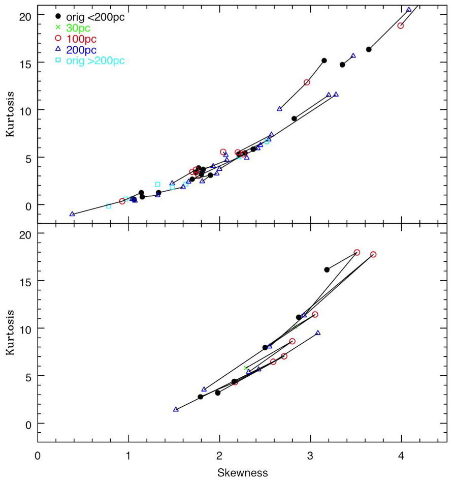
Figure 5: Kurtosis versus skewness measured over the entire H i moment 0 maps of the galaxies. Pixels with $N_{HI}$ $\leq 15\times 10^{18}$ cm^-2 were eliminated to ensure good S/N. Values are plotted for the original H i maps, with separate symbols for beam-sizes that have major axes that are $<$200 pc in size (“orig $<$200pc”) and those with beam-sizes that are $>$200 pc (“orig $>$200 pc”). Values are also plotted for maps smoothed to 30 pc, 100 pc, and 200 pc beam-sizes, where possible. Original beam-sizes that are close to one of the smoothed values are plotted with the smoothed symbol and color. The solid black lines connect different maps of the same galaxy in order to facilitate comparison of values at different map spatial resolutions. NGC 1569 at 200 pc resolution, with a kurtosis value of 38, is not plotted. Bottom panel shows those galaxies where skewness and kurtosis values do not decline as the beam-size increases: DDO 69, DDO 75, DDO 187, DDO 210, IC 10, UGC 8508, WLM.

We have measured the skewness and kurtosis values for the entire H i distributions of each galaxy. Pixels with $N_{HI}$ $\leq 15\times 10^{18}$ cm^-2 were eliminated to ensure good S/N. Values were measured on the original integrated H i maps and on maps smoothed to beam-sizes of 30 pc, 100 pc, and 200 pc, where possible. Values for all maps are given in Table 2 and plotted in Figure 5 where different maps for the same galaxy are connected with a solid black line. We see that, for a given galaxy, generally skewness and kurtosis values decline as the beam-size increases. This makes sense: as the beam-size increases peaks and valleys in the H i column density distributions get smoothed out and so the deviations from the average decrease in amplitude. However, there are some exceptions where kurtosis values increase as beam-size increases, and in some cases, then decrease for the highest beam size of 200 pc: DDO 69, DDO 75, DDO 187, DDO 210, IC 10, UGC 8508, WLM. As a whole, the results for beam-sizes $>$200 pc fall in the left hand corner of Figure 5 (skewness $<2.6$ and kurtosis $<7$), but results for beam-sizes $\sim$200 pc and $\sim$100 pc are found throughout the full range of values. Values for the two galaxies smoothed to 30-pc beam-sizes fall in the middle of the range shown in Figure 5. Here we will compare galaxies with comparable beam-sizes.

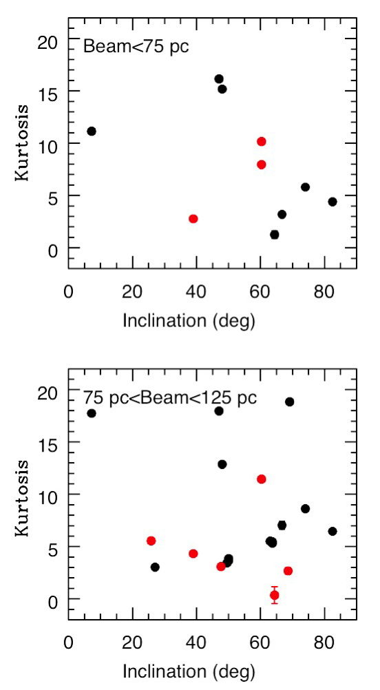
Figure 6: Kurtosis measured over the entire H i moment 0 maps of the galaxies plotted against inclination of the disk. The inclinations are given by Oh et al. (2015) for galaxies marked with an “H” in Figure 2 (black points) and by Hunter & Elmegreen (2006) for galaxies marked with an “O” in Figure 2 (red points). Pixels with $N_{HI}$ $\leq 15\times 10^{18}$ cm^-2 were eliminated to ensure good S/N. Maps with beam-sizes $<$75 pc are plotted in the upper panel, and maps with beam-sizes 75 pc to 125 pc are plotted in the lower panel. Maps with beam-sizes $>$125 pc are not plotted here. We do not see a significant effect of inclination, and its effect on angular resolution, on kurtosis values.

Another factor that could potentially affect spatial resolution is the inclination of the galaxy. The more inclined the disk is, the more material a given sight-line is integrating over and so the effective spatial resolution is lower. In Figure 6 we plot the galaxy-wide kurtosis values against inclination of the H i disk. We have grouped the galaxies into beam-sizes: $<$75 pc and 75 pc to 125 pc. Galaxies with beam-sizes larger than 125 pc are not included in this plot. Note that black points were determined using inclinations derived from the H i kinematics and red points from the optical morphology. We differentiate them in order to show that there is no trend with type of inclination determination. If inclination is a significant factor, we would expect kurtosis values to be higher for more face-on systems. In the upper panel, where the maps with beam-sizes $<$75 pc are plotted, we see such a trend in the upper envelope of points. However, there is a large scatter in kurtosis values for inclinations $\leq$60°. In the bottom panel, where maps with beam-sizes 75 pc to 125 pc are plotted, we see a general scatter of kurtosis values with no trend. From these plots, we conclude that inclination could be a factor in the highest resolution maps, but that this does not affect our results any more than comparing galaxies over our range in resolutions.

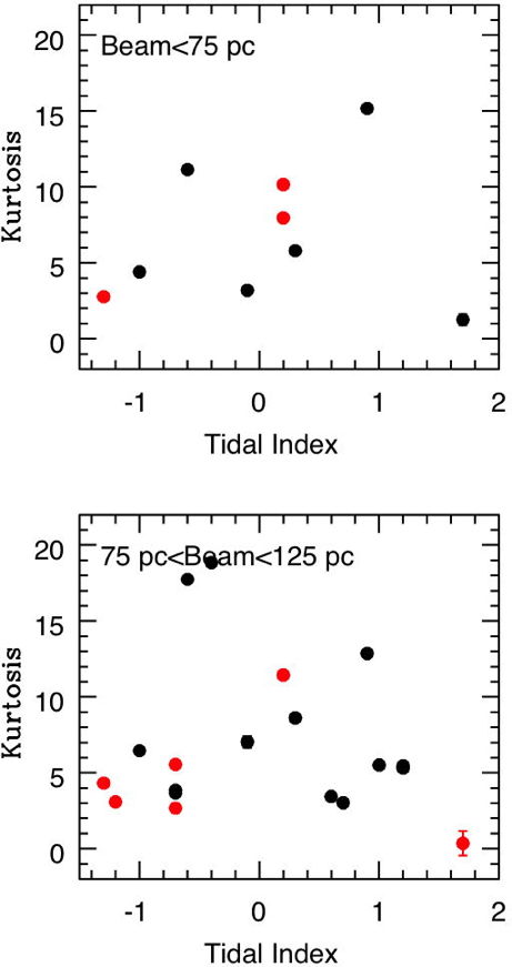
Figure 7: Kurtosis measured over the entire H i moment 0 maps of the galaxies plotted against the tidal index of the galaxy from Karachentsev et al. (2004) as given by Zhang et al. (2012). The larger the tidal index, the stronger the gravitational disturbance exerted by neighboring galaxies. Nearly isolated galaxies have zero or negative values. Black points are galaxies marked with an “H” in Figure 2 and red points are galaxies marked with an “O” in Figure 2. Pixels with $N_{HI}$ $\leq 15\times 10^{18}$ cm^-2 were eliminated to ensure good S/N. Maps with beam-sizes $<$75 pc are plotted in the upper panel, and maps with beam-sizes 75 pc to 125 pc are plotted in the lower panel. Maps with beam-sizes $>$125 pc are not plotted here. We do not see a correlation of kurtosis with tidal index.

One difference between the LITTLE THINGS dwarfs and the SMC is their relative isolation. The LITTLE THINGS dwarfs were chosen to be relatively far from other galaxies, especially giant systems, and not (obviously) engaged in an interaction with another galaxy. On the other hand, the SMC is clearly interacting with the LMC and the Milky Way. Burkhart et al. (2010) suggest that high skewness and kurtosis values could result from large-scale gravitational effects in a galaxy-galaxy interaction. The tidal index, computed by Karachentsev et al. (2004) and collected by Zhang et al. (2012) for the LITTLE THINGS sample, is a measure of the strength of gravitational disturbance exerted by neighboring galaxies. Nearly isolated galaxies have zero or negative values, and the LITTLE THINGS sample has tidal indices ranging from -1.3 to 1.7. In Figure 7 we plot kurtosis measured over the entire H i moment 0 maps of the galaxies against the tidal index of the galaxy. We do not see a correlation of galaxy-wide kurtosis with tidal index.

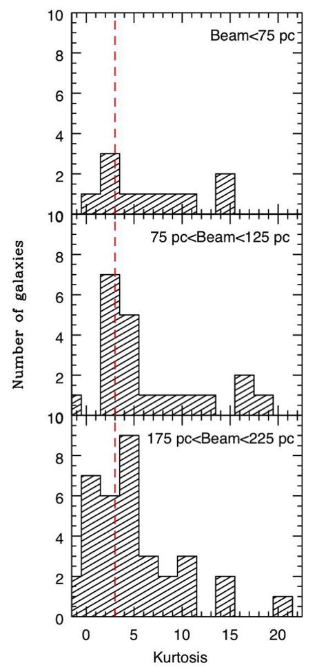
Figure 8: Number of galaxies with certain kurtosis values measured over the entire H i moment 0 maps of the galaxies. Pixels with $N_{HI}$ $\leq 15\times 10^{18}$ cm^-2 were eliminated to ensure good S/N. The maps are grouped by beam-size: beam-size $<$75 pc, beam-size between 75 pc and 125 pc, and beam-size between 175 pc and 225 pc. A galaxy in the top panel will also appear in the middle and bottom panels, and a galaxy that appears in the middle panel will also appear in the bottom panel. NGC 1569 at 200 pc resolution, with a kurtosis value of 38, is not plotted. The vertical red, dashed line marks a kurtosis value of 3; above this value the gas is supersonic according to the models of Burkhart et al. (2010). Most (60%) of the galaxies have kurtosis values $\leq 5$ regardless of angular resolution of the map, but numbers range up to 19.

Figure 8 shows a histogram of kurtosis values with maps grouped by beam-size: $<$75 pc, between 75 pc and 125 pc, between 175 pc and 225 pc. We see that typical values of kurtosis are $\leq 5$, and 60% of the sample has values in this range. These values are comparable to the kurtosis value of 2.5 measured by Burkhart et al. (2010) for the SMC and values measured in spiral galaxies (Maier et al., 2016). The rest of the systems have kurtosis values that range from 5 up to 19.

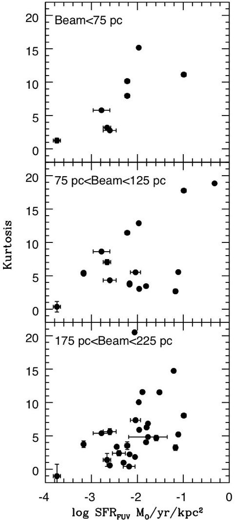
Figure 9: Kurtosis values measured over the entire H i moment 0 maps of the galaxies versus integrated SFR determined from the FUV (Hunter et al., 2010). Uncertainties are shown in both quantities but in many cases the uncertainties are smaller than the point symbol. Pixels with $N_{HI}$ $\leq 15\times 10^{18}$ cm^-2 were eliminated to ensure good S/N. The maps are grouped by beam-size: beam-size $<$75 pc, beam-size between 75 pc and 125 pc, and beam-size between 175 pc and 225 pc. A galaxy in the top panel will also appear in the middle and bottom panels, and a galaxy that appears in the middle panel will also appear in the bottom panel. NGC 1569 at 200 pc resolution, with a kurtosis value of 38, is not plotted. There is a general trend of higher kurtosis values for higher SFR.

Figure 9 shows kurtosis values plotted against integrated galactic star formation rates (SFRs) determined from the FUV (Hunter et al., 2010). Again, maps are grouped by beam-size, which determines the spatial resolution: $<$75 pc, between 75 pc and 125 pc, between 175 pc and 225 pc. Although there is a lot of scatter, there is a general trend of higher SFRs being accompanied by higher kurtosis values at all three spatial resolutions. We expect higher turbulence to be associated with the energy input from star forming regions (for example, in the ionized gas, Moiseev et al., 2015), and we expect highly turbulent regions to produce more star formation in compressed shells and other structures (Dopita et al., 1985).

3.2.2 Radial variations

To look at how kurtosis might vary with radius in galaxies, we have selected a subsample of galaxy maps that were chosen to have at least 20 beam-sizes along the semi-major axis. This ensures that annuli can be constructed in which there are enough independent beams to determine a statistically significant kurtosis value. The radii were chosen to be 6, 8.5, 10.5, 12.5, 14, 15.5, etc. times the beam major axis. This gives at least 100 beam areas per annulus, assuming every pixel has emission. To maximize resolution, we use the original unsmoothed H i maps, except for IC 10 and IC 1613 for which we use the 30-pc beam maps. We also eliminated pixels with values less than $15\times 10^{18}$ cm^-2 for S/N, and eliminated radii where the number of pixels is such that the uncertainty in kurtosis exceeds 1. The uncertainty is based on the number of beam areas included in the pixels with emission.

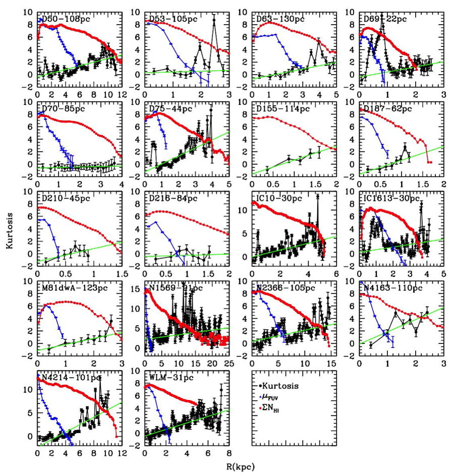
Figure 10: Kurtosis values measured in elliptical annuli versus the radii of the midpoints of the annuli. Pixels with $N_{HI}$ $\leq 15\times 10^{18}$ cm^-2 were eliminated to ensure good S/N. Only galaxies with maps in which there are at least 20 beam-sizes along the semi-major axis were included. The average of the major and minor axes of the beam size are given next to the galaxy name in each panel. The ellipse parameters (center, inclination and minor-to-major axis ratio, position angle of the major axis) are given by Oh et al. (2015) for galaxies marked with an “H” in Figure 2 and by Hunter & Elmegreen (2006) for galaxies marked with an “O” in Figure 2. We see no correlation between features in the kurtosis profiles and those in the FUV profiles. Green lines are linear fits to the kurtosis profiles, not including spikes.

Radial plots of kurtosis profiles and FUV surface photometry $\mu_{FUV}$ are shown in Figure 10. We see a variety of kurtosis profiles. In three galaxies (DDO 70, DDO 210, DDO 216) the kurtosis values are predominantly flat with radius and in 7 (DDO 50, DDO 155, DDO 187, IC 10, M81dwA, NGC 4163, WLM) there is a gradual increase of kurtosis with radius. In 5 galaxies (DDO 53, DDO 63, DDO 75, NGC 2366, NGC 4214) there are particularly high values in the outer disk and in three others (DDO 69, IC 1613, NGC 1569) there are spikes in kurtosis closer in to the center of the galaxy. We also see that kurtosis and $\mu_{FUV}$, which is proportional to the recent star formation activity, are not related in the azimuthal-averaged annuli. This is in spite of the fact that we found a general trend of higher SFR with kurtosis for galaxy-wide integrated values in Figure 9 for galaxies with beam-sizes less than 75 pc. The trend of increasing kurtosis with radius is partly the result of a change in the ratio of the maximum value of $N(HI)$ in each annulus divided by the value at the peak of the PDF, as discussed in Section 4.

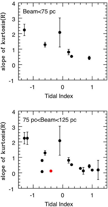
Figure 11: Slope of a linear fit to kurtosis radial profiles (Figure 10) against the tidal index of Karachentsev et al. (2004). We have eliminated the spikes in kurtosis from the fits. The fits are shown in green in Figure 10. Nearly isolated galaxies have zero or negative tidal indices. The one known interacting system in these plots, NGC 1569, is plotted in red. We find a general trend in the sense that a higher tidal index generally means a more constant kurtosis value with radius.

We explore the possible effects of nearby neighbors in Figure 11, where we plot the slope of a linear fit to kurtosis as a function of radius against the tidal index of Karachentsev et al. (2004). We have eliminated spikes in kurtosis for the fits. The fits are shown as green lines in Figure 10. Nearly isolated galaxies have zero or negative tidal indices, so most of the galaxies would be considered isolated. The one known interacting system in these plots, NGC 1569, is plotted in red and it has a tidal index of -0.4, so it too would be considered isolated. We do find a general trend in the sense that a higher tidal index means a more constant kurtosis value with radius.

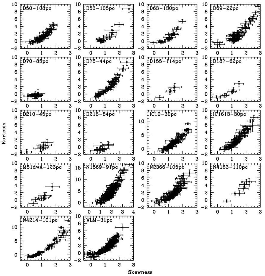
Figure 12: Kurtosis values plotted against skewness values measured in elliptical annuli. Pixels with $N_{HI}$ $\leq 15\times 10^{18}$ cm^-2 were eliminated to ensure good S/N. Only galaxies with maps in which there are at least 20 beam-sizes along the semi-major axis were included. The average of the major and minor axes of the beam size are given next to the galaxy name in each panel. The ellipse parameters (center, inclination and minor-to-major axis ratio, position angle of the major axis) are given by Oh et al. (2015) for galaxies marked with an “H” in Figure 2 and by Hunter & Elmegreen (2006) for galaxies marked with an “O” in Figure 2. Most (72%) of the 18 galaxies show a strong correlation between kurtosis and skewness values.

In Figure 12 we plot kurtosis versus skewness for each annulus. For 72% of the sample of 18, we see a strong correlation between skewness and kurtosis, with kurtosis values ranging from about $-1$ to 17 and skewness values ranging from about 0 to 4. The exceptions are DDO 70, DDO 155, DDO 210, DDO 216, and M81dwA, where the annuli clump around kurtosis and skewness values of 0-2.

3.2.3 Kernel analysis

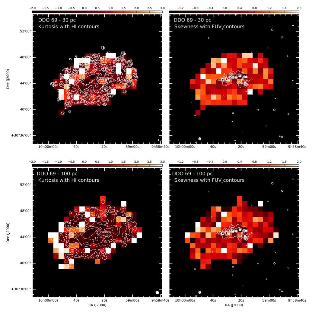
Figure 13: Maps of kurtosis (left) with contours of integrated H i and of skewness (right) with contours of FUV. The kurtosis and skewness maps are determined in contiguous kernels or cells that are 32 of the H i map pixels $\times$ 32 pixels in size, so each square in these images is one kernel. The size of the kernel in parsecs is given in Table 3. H i map beam-size is indicated as a solid white ellipse in the right corner of the left image, and is given in parsecs next to the galaxy name in the upper left. The H i contours are 5, 30, 100, 300, 500, 1000, and $3000\times 10^{18}$ atoms cm^-2, except for DDO 50, IC 1613, NGC 1569, and WLM for which the 30 and $300\times 10^{18}$ atoms cm^-2 contours are left out. The kurtosis and skewness maps show little correlation with star formation as seen in the FUV.

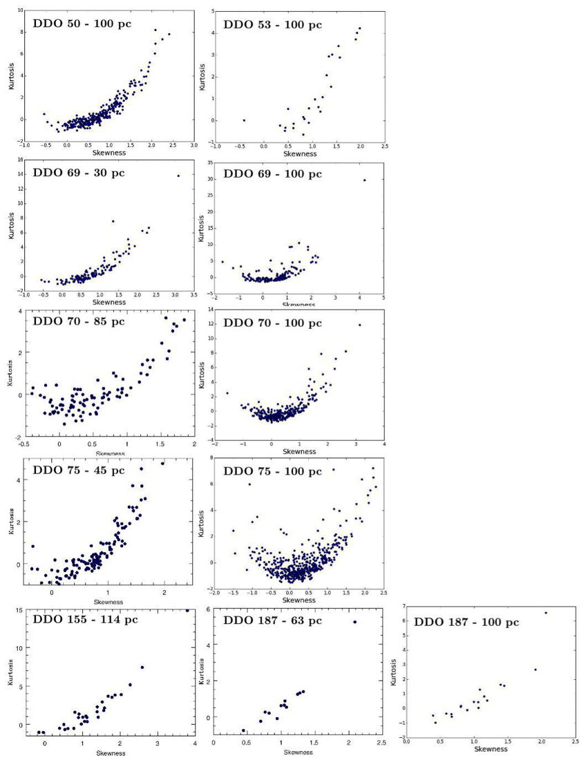
Figure 14: Kurtosis values versus skewness values for 32 pixel $\times$ 32 pixel kernels. The beam size of the H i map is given next to the galaxy name in each plot. For maps with the original beam, the given beam size is the average of the major and minor axes of the beam. For smoothed maps, the minor and major axes are the same. We assume that the higher angular resolution maps of these galaxies are a better indication of gas turbulence. Many of the galaxies show a strong correlation between kurtosis and skewness among the kernels.

We selected a sub-sample of H i maps for kernel analysis. In particular, we chose galaxies with beam sizes of order 100 pc or less in order to have high angular resolution, but included all maps — original beam and smoothed beams — of the galaxy up to a beam-size of 100 pc to allow comparison of resolution effects. We also eliminated galaxies that were too small to contain a reasonable number of kernels. The final sub-sample is given in Table 3. For these galaxies, we divided the H i maps into a grid of adjacent, contiguous kernels or cells (for more details, see Maier et al., 2016). Each kernel is 32 of the H i map pixels $\times$ 32 pixels, where the H i map pixel is 1.5″$\times$1.5″ except in DDO 216 where the pixel size is 3.5″$\times$3.5″. Typically the original beam-size is several H i map pixels across. The equivalent of a 32-pixel length in parsecs is given in Table 3 for each galaxy. We normalized the column densities and calculated skewness and kurtosis values of the H i distributions within each kernel. Then we constructed maps of skewness and kurtosis in which the 32 pixel $\times$ 32 pixel area of the original map is replaced by a single kurtosis or skewness value. We geometrically converted FUV images to match the scale and orientation of the H i maps, measured the FUV magnitude in each kernel, and constructed an FUV map for comparison to the H i higher order moments. These maps are shown in Figure 13. Each square in these images is one kernel. For each map of each galaxy, we also plotted skewness versus kurtosis for the ensemble of kernels, one point per kernel. These plots are shown in Figure 14.

For DDO 69, IC 1613, and WLM, in Figure 13 we show the maps produced from 30 pc and 100 pc beam-size maps. For the most part, the maps are the same, regardless of resolution. The exception is the skewness map of WLM that shows a difference in skewness values between the inner and outer galaxy in the 30-pc map that is not seen in the 100-pc map. The rest of the galaxy maps are based on the 100-pc beam-size maps. We see that for most of the galaxies, the skewness and kurtosis values are fairly uniform across the galaxy. However, sometimes (DDO 50, DDO 69, DDO 70, IC1613, WLM, NGC 2366, NGC 4214) there is a general increase in skewness values around the edges of the galaxy, which we also found for spiral galaxies (Maier et al., 2016). Also as we saw in spiral galaxies, most often there is not a noticeable correlation of kurtosis or skewness values with FUV features. However, DDO 50, IC 1613, and WLM do show a small correlation.

In the skewness versus kurtosis plots (Figure 14), a comparison of different beam-sizes for a given galaxy (DDO 69, DDO 70, DDO 75, IC 1613, WLM; DDO 187 does not have enough points) shows that a map with lower spatial resolution tends to show a poorer correlation of skewness with kurtosis, while the higher resolution map tends show more of a correlation. The exceptions are DDO 70 and IC 1613, which show a poor correlation at both resolutions. Presumably the higher resolution beams are a more accurate indication of the motions of the gas in the galaxy. Of the rest of the galaxies (excluding DDO 216 for the limited number of points), DDO 50, DDO 53, DDO 155, DDO 210, IC 10, NGC 1569, NGC 2366, and NGC 4214 show a strong correlation between kurtosis and skewness with most values ranging from -1 to 8 for kurtosis and -0.5 to 3 for skewness. A few kernels have kurtosis values as high as 30. In all, of the 13 galaxies in the kernel sample 69% show a correlation between kurtosis and skewness among all the kernels. Of the 8 galaxies showing a strong correlation between kurtosis and skewness among the kernels, one did not show such a pattern in the annuli (DDO 210) and a second did not have enough points for a determination (DDO 155, Figure 12). Of the 5 galaxies showing weak correlations among the kernels, one also did not show a correlation among annuli (DDO 70). Thus, for the most part, the annuli results and the kernel results are similar with respect to correlations between kurtosis and skewness.

4 Discussion

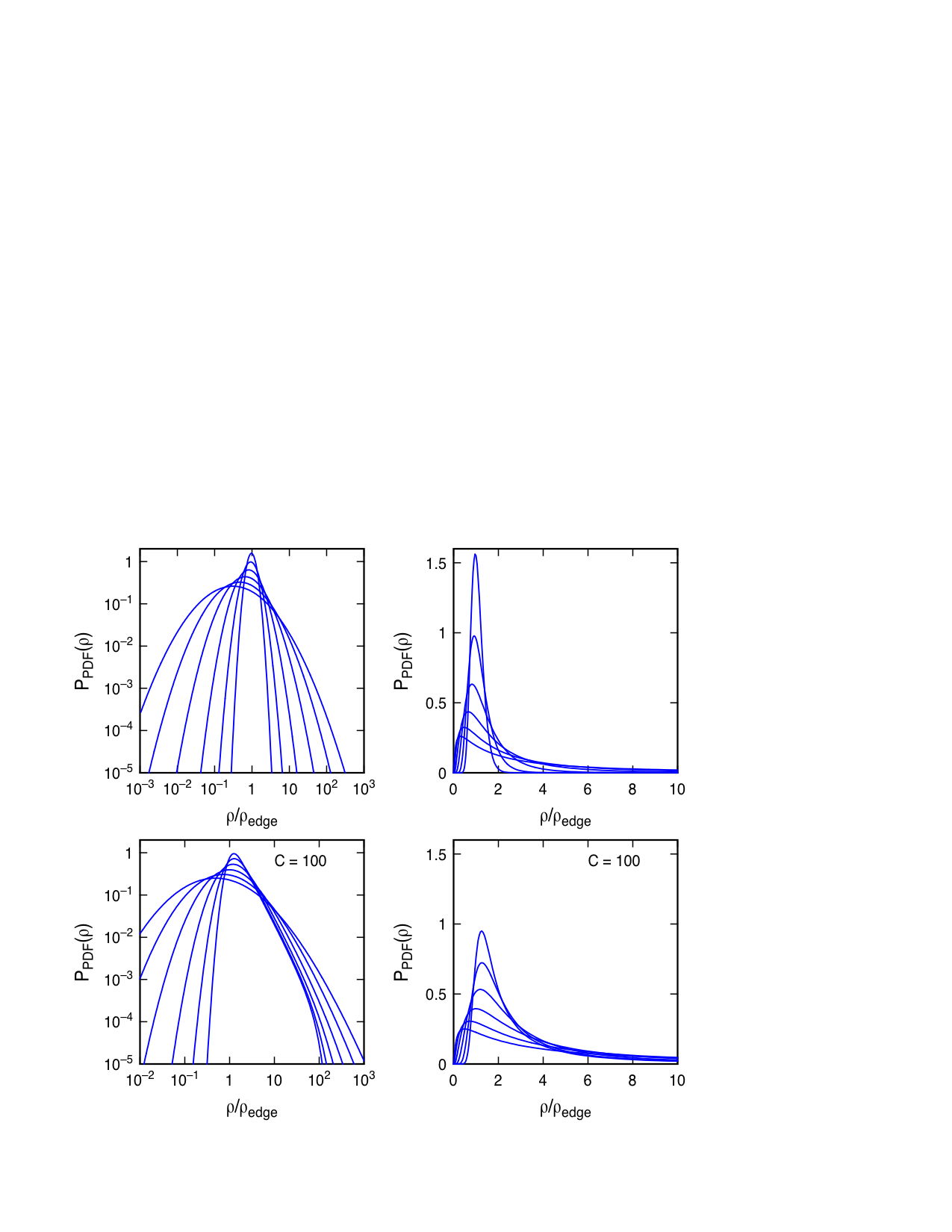
Figure 15: Top: Density PDFs in the pure log-normal case from equations (2)-(4) for Mach numbers of 0.52, 0.85, 1.40, 2.29, 3.76, and 6.17 as a sequence of increasing width. On the left, the PDFs are plotted in log-log coordinates and on the right they are plotted in linear coordinates. The tail responsible for kurtosis and skew is always present, and it gets relatively larger for wider log-normal functions. Bottom: PDFs for the same Mach numbers, now using equation (5) with a ratio of average-to-edge density, ${\cal C}$, equal to 100. For small Mach numbers, the power-law density profile dominates the PDF and the high-density side becomes nearly a power law. For large Mach numbers, the log-normal still dominates in the high-density side and the PDF remains curved in log-log coordinates. On the right, the same distributions are plotted in linear coordinates.

The PDF of interstellar column density is close to log-normal in the solar neighborhood (Lombardi et al., 2010), as expected for compressive turbulence (Vázquez-Semadeni, 1994; Passot & Vázquez-Semadeni, 1998; Padoan, Nordlund & Jones, 1997; Lemaster & Stone, 2008; Federrath et al., 2010). A log-normal is a Gaussian distribution in the logarithm of the column density. When the ISM column densities are replotted on a linear scale, there is a fat tail at high $N_{HI}$ which contains the same information about turbulence as the original log-normal. This fat tail is shown in Figure 15. The top two panels have log-normal distribution functions, evaluated as discussed below, with 6 different widths and normalized by area. On the left these functions are plotted in log coordinates, and on the right the same functions are plotted in linear coordinates. The tail at high density on the linear plot gets larger relative to the peak of the distribution function as the log-normal width increases. The bottom two panels show distribution functions with 6 widths and convolved with power law tails, simulating turbulence in self-gravitating clouds (Eq. 5 below).

In a physical model of turbulence, the tail is caused by numerous tiny compressed regions. For an intrinsically log-normal function, the tail results in skewness and kurtosis in the linear distribution. Skewness and kurtosis tend to increase with Mach number because the dispersion in a log-normal PDF increases with Mach number (Padoan, Nordlund & Jones, 1997). They also increase when the maximum value of $N(HI)$ in the distribution function increases relative to the value at the peak of the function because that extends the measured part of the fat tail further.

We model the dependence of kurtosis on skewness to reproduce Figures 5, 12, and 14 by constructing log-normal distribution functions and measuring their skewness and kurtosis on a distribution with linear coordinates as we did for the observations. We consider two types of PDF functions, written in terms of spatial density; they are considered to be approximately the same shape for column density. One is a pure log-normal as shown on the top of Figure 15,

$$P(\ln\rho)d\ln\rho=(2\pi D^{2})^{-1/2}e^{-0.5\left(\ln(\rho/\rho_{\rm pk})/D\right)^{2}}$$ (2)

where the density at the peak, $\rho_{\rm pk}$, is related to the average density by

$$\rho_{\rm pk}=\rho_{\rm ave}e^{-0.5D^{2}},$$ (3)

and the dispersion, D, is related to the Mach number, M, by (Padoan, Nordlund & Jones, 1997)

$$D^{2}=\ln(1+0.25{\cal M}^{2}).$$ (4)

The second PDF is a log-normal modified by a power law at high density, which is appropriate for self-gravitating clouds (Kritsuk, Norman & Wagner, 2011). We use the formalism in Elmegreen (2011) where the final PDF is the convolution of a power law radial density profile in a self-gravitating cloud with a log-normal distribution locally inside the cloud for the average density at that position. The Mach number is assumed to be constant inside the cloud. This gives (see Elmegreen, 2011)

$$P_{\rm PDF,total}(y)={{3{\cal C}}\over{\alpha(2\pi)^{0.5}}}\int_{1/{\cal C}}^{1}\exp\left(-{{\ln^{2}(yze^{0.5D^{2}})}\over{2D^{2}}}\right){{\left(z{\cal C}-1\right)^{(3-\alpha)/\alpha}}\over{D\left({\cal C}-1\right)^{3/\alpha}}}dz,$$ (5)

per unit $\ln y$, where $y=\rho/\rho_{\rm edge}$ is the local normalized density, including turbulent fluctuations, and $z=\rho_{\rm edge}/\rho_{\rm ave}(r)$ is the inverse of the average density, not including the turbulent fluctuations, both normalized to the density at the edge of the cloud, $\rho_{\rm edge}$. The average density is assumed to vary with radius as a cored power-law to simulate the effects of self-gravity,

$$\rho_{\rm ave}(r)=\rho_{\rm edge}{{r_{\rm edge}^{\alpha}+r_{\rm core}^{\alpha}}\over{r^{\alpha}+r_{\rm core}^{\alpha}}}.$$ (6)

The core radius, $r_{\rm core}$, avoids a density singularity. The degree of central condensation,

$${\cal C}={{\rho_{\rm ave}(r=0)}\over{\rho_{\rm edge}}},$$ (7)

is varied to simulate how strongly self-gravitating the cloud is.

The kurtosis and skewness of a distribution function with a fat tail depend sensitively on the upper limit for $N(HI)$. We modify these PDFs to include upper and lower density cutoffs by converting the density in the equation to a density of observation using

$$\rho_{\rm obs}={{1}\over{1/\rho+1/\rho_{\rm upper}}}$$ (8)

if $\rho>\rho_{\rm ave}$, and

$$\rho_{\rm obs}=\rho+\rho_{\rm lower}$$ (9)

if $\rho<\rho_{\rm ave}$, and where $\rho_{\rm lower}=0.01$ and $\rho_{\rm upper}=10$ and 100 in two cases. At large $\rho$ the observed density converges to the constant value $\rho_{\rm upper}$, which is interpreted as the limiting density before molecules form. Higher density gas shows this limiting density from H i in the shielding layer. Below $\rho_{\rm lower}$, the H i is assumed to disappear because of ionization and heating in a hot medium. Phase transitions like this were also necessary to fully characterize the pdf of H i column density in the LMC (Elmegreen et al., 2001).

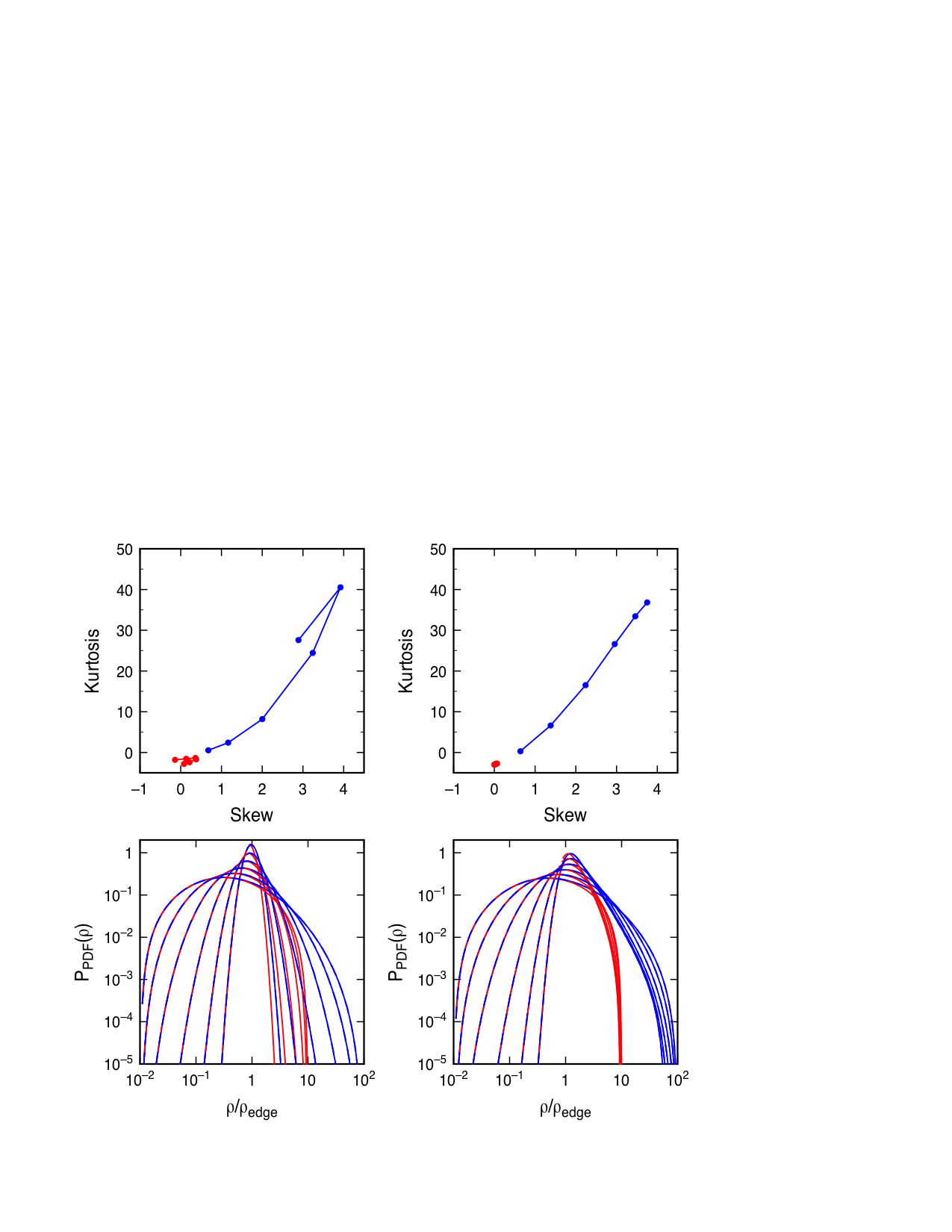
Figure 16: Kurtosis model. Bottom left: Density PDFs in the pure log-normal case for Mach numbers of 0.52, 0.85, 1.40, 2.29, 3.76, and 6.17 as a sequence of increasing width, and for $\rho_{\rm upper}=10$ (red), 100 (blue). The curves are dashed blue and red for low $\rho$ because the functions are the same for the two values of $\rho_{\rm upper}$. Top left: Kurtosis versus the skewness, using the same colors. Kurtosis and skewness both increase with Mach number, and they have the same relationship as in Figures 5, 12, and 14, keeping in mind that the models are for density and the observations are of column density. Right: Density PDFs, kurtosis, and skewness for the self-gravitating model with center-to-edge contrast ${\cal C}=100$, using the same Mach numbers and upper limits as on the left.

The bottom left-hand side of Figure 16 shows the density PDFs in the non-gravitating case for Mach numbers of 0.52, 0.85, 1.40, 2.29, 3.76, and 6.17 as a sequence of increasing width, and for $\rho_{\rm upper}=10$ (red) and 100 (blue). The kurtosis versus skewness is shown in the top-left, using the same colors. Kurtosis and skewness both increase with Mach number at first and then decrease again for the largest Mach number. They have the same relationship to each other as in Figures 5, 12, and 14, keeping in mind that the models are for density and the observations are of column density. The observations span a range in PDF values that is a factor of $10^{2}$-$10^{3}$ on the vertical axis (Fig. 2), so the distinction between the $\rho_{\rm upper}=10$ and 100 models is not clear in Figure 16 (we can rule out $\rho_{\rm upper}=1000$ because it is too broad).

The right-hand side of Figure 16 shows density PDFs, kurtosis, and skewness for the self-gravitating model with center-to-edge contrast ${\cal C}=100$, using the same Mach numbers and lower and upper limits as on the left. The self-gravitating model is also a good match to the observations, although in this case, the kurtosis and skew decrease with increasing Mach number for $\rho_{\rm upper}=100$.

The change in kurtosis with Mach number is a result of a change in the PDF close to the peak. For the non-gravitating case, the PDF is symmetric in log-log coordinates, so increasing Mach number simply increases the strength of the tail, and with it the kurtosis. In the gravitating case, the power-law part from the radial gradient of density in the cloud is more prominent at low Mach number because then turbulence does not interfere as much with the power law. This is the most asymmetric case near the peak because the power law at high density makes the tail stronger relative to the lower density part. At higher Mach number the turbulence dominates the power law and the PDF becomes more curved, as in the non-gravitating case. Then the kurtosis decreases with increasing Mach number.

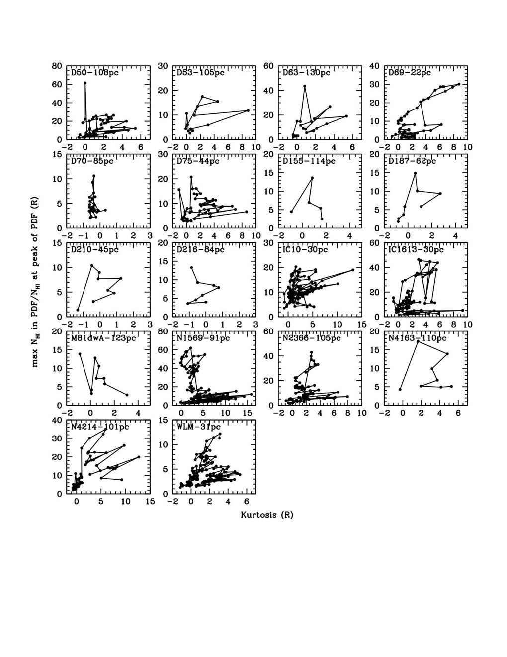
Figure 17: The ratio of the maximum value of $N(HI)$ in each annulus to the value at the peak of the PDF in that annulus, versus kurtosis for the same annulus. Each point is a different annulus and the points are connected by line segments for increasing radius. Excursions toward high ratios of column density often correspond to high values of kurtosis, indicating that kurtosis depends partly on how far out the H i can be observed in the PDF tail before it disappears or converts to molecules.

Figure 16 suggests that the range of kurtosis and skewness observed for dIrr galaxies is the result of variations in the Mach number combined with a variable upper limit to the column density from the conversion of atomic to molecule gas. The effect of the upper limit to $N(HI)$ may dominate the radial variation in the kurtosis shown in Figure 10. We plotted (not shown) the ratio of the maximum value of $N(HI)$ to the value at the peak of the PDF in each radial annulus versus the radius of the annulus. The radial distribution of rising or flat values for this ratio resembled the trends of kurtosis in Figure 10. This implies that there is a correlation between kurtosis and the observational cutoff in the fat tail. Figure 17 shows this correlation more directly for each galaxy in Figure 10. The interconnected points in the figure are the values for each annulus traced over increasing radius. There is a tendency for simultaneous excursions on each axis, although the slopes of these excursions vary from galaxy to galaxy and sometimes have two values inside any given galaxy.

5 Summary

We have presented PDFs and higher order moment (skewness and kurtosis) analysis of the integrated H i column density distributions in the LITTLE THINGS sample of nearby dIrr galaxies. This analysis follows that of Burkhart et al. (2010) for the SMC. We find that galaxy-wide values of kurtosis are similar to that found for the SMC for about 60% of our sample, with values ranging as high as 19. The kurtosis values for whole galaxy PDFs roughly correlate with integrated SFRs such that higher SFRs correspond more often to higher kurtosis values. Kurtosis and skewness values calculated for annuli within a subsample of 18 galaxies with beam-sizes less than or equal to 130 pc most often (72%) show a correlation between kurtosis and skewness values with no correlation with the FUV radial profile. We also analyzed a grid of 32 pixel $\times$ 32 pixel kernels (160 pc $\times$ 160 pc to 840 pc $\times$ 840 pc areas) in the 30-pc and 100-pc maps of a subsample of 13 galaxies. There we also found a correlation of kurtosis with skewness for many of the galaxies with most kurtosis values ranging from $-1$ to 8, especially at the highest resolution, where small H i peaks at high density could be resolved. However, there was no correlation with local FUV features.

These results are consistent with a model where the typical dIrr galaxy has a turbulent multi-phase ISM with subsonic to weakly supersonic motions that are excited on scales larger than the local star-forming regions but still related to the integrated star formation rate. Higher spatial resolution shows more H i substructure and suggests higher Mach numbers.

The distribution functions for the maximum values of $N_{HI}$ in four radial intervals show a decreasing trend with radius that suggests H i disappears at high density by conversion to molecules at a column density determined by the balance between H₂ formation on grain surfaces and H₂ destruction by ambient radiation. Aside from the innermost radii in a few galaxies, the H i column of gas rarely becomes optically thick to UV radiation from dust extinction, but converts to H₂ because of self-shielding when it is still optically thin. As a result, molecule formation is sensitive to local pressure and radiation. We find that the shielding envelopes of the H₂ clouds could be in pressure equilibrium with the general interstellar medium. Because all radial intervals have star formation and therefore dense gas, and essentially all of the H i column densities peak in optically thin gas, there should be a substantial amount of diffuse H₂ in these galaxies, with conversion to CO possibly limited to the dense cores where stars actually form.

Models of log-normal density PDFs or log-normals convoluted with a power law to simulate self-gravitating clouds were used to explain the observed trends between kurtosis and skewness as a result of variations in the PDF width, which is related to Mach number and the upper HI cutoff where presumably molecules form. Kurtosis and skewness in linear PDFs for $N_{HI}$ are expected because of the conversion in plotting coordinates from log-log to linear-linear.

Table 1: Galaxies and basic data

	D	$R_{D}$	$R_{Br}$		$\log{SFR}_{D}^{FUV}$
Galaxy	(Mpc)	(kpc)	(kpc)	$M_{V}$	(M${}_{\sun}\;$ yr-1 kpc-2)	log O/H+12
CvnIdwA	3.6	0.25$\pm$0.12	0.56$\pm$0.49	-12.37$\pm$0.07	-1.77$\pm$0.42	$7.3\pm 0.06$
DDO 43	7.8	0.87$\pm$0.10	1.46$\pm$0.53	-15.06$\pm$0.02	-2.20$\pm$0.10	$8.3\pm 0.09$
DDO 46	6.1	1.13$\pm$0.05	1.27$\pm$0.18	-14.67$\pm$0.01	-2.45$\pm$0.04	$8.1\pm 0.1$
DDO 47	5.2	1.34$\pm$0.05	$\cdots$	-15.46$\pm$0.01	-2.38$\pm$0.03	$7.8\pm 0.2$
DDO 50	3.4	1.48$\pm$0.06	2.65$\pm$0.27	-16.61$\pm$0.00	-1.81$\pm$0.04	$7.7\pm 0.14$
DDO 52	10.3	1.26$\pm$0.04	2.80$\pm$1.35	-15.45$\pm$0.03	-2.53$\pm$0.03	(7.7)
DDO 53	3.6	0.47$\pm$0.01	0.62$\pm$0.09	-13.84$\pm$0.01	-1.96$\pm$0.02	$7.6\pm 0.11$
DDO 63	3.9	0.68$\pm$0.01	1.31$\pm$0.10	-14.78$\pm$0.02	-2.05$\pm$0.02	$7.6\pm 0.11$
DDO 69	0.8	0.19$\pm$0.01	0.27$\pm$0.05	-11.67$\pm$0.01	-2.22$\pm$0.05	$7.4\pm 0.10$
DDO 70	1.3	0.44$\pm$0.01	0.13$\pm$0.07	-14.10$\pm$0.00	-2.17$\pm$0.02	$7.5\pm 0.06$
DDO 75	1.3	0.18$\pm$0.01	0.71$\pm$0.08	-13.91$\pm$0.01	-0.99$\pm$0.05	$7.5\pm 0.06$
DDO 87	7.7	1.21$\pm$0.02	0.99$\pm$0.11	-14.98$\pm$0.02	-2.61$\pm$0.02	$7.8\pm 0.04$
DDO 101	6.4	0.97$\pm$0.06	1.16$\pm$0.11	-15.01$\pm$0.01	-2.84$\pm$0.05	$8.7\pm 0.03$
DDO 126	4.9	0.84$\pm$0.13	0.60$\pm$0.05	-14.85$\pm$0.01	-2.18$\pm$0.13	(7.8)
DDO 133	3.5	1.22$\pm$0.04	2.25$\pm$0.24	-14.76$\pm$0.01	-2.60$\pm$0.03	$8.2\pm 0.09$
DDO 154	3.7	0.48$\pm$0.02	0.62$\pm$0.09	-14.19$\pm$0.01	-1.77$\pm$0.04	$7.5\pm 0.09$
DDO 155	2.2	0.15$\pm$0.01	0.20$\pm$0.04	-12.53$\pm$0.02	$\cdots$	$7.7\pm 0.06$
DDO 165	4.6	2.24$\pm$0.08	1.46$\pm$0.08	-15.60$\pm$0.01	$\cdots$	$7.6\pm 0.08$
DDO 167	4.2	0.22$\pm$0.01	0.56$\pm$0.11	-12.98$\pm$0.04	-1.59$\pm$0.04	$7.7\pm 0.2$
DDO 168	4.3	0.83$\pm$0.01	0.72$\pm$0.07	-15.72$\pm$0.01	-2.06$\pm$0.01	$8.3\pm 0.07$
DDO 187	2.2	0.37$\pm$0.06	0.28$\pm$0.05	-12.68$\pm$0.01	-2.60$\pm$0.14	$7.7\pm 0.09$
DDO 210	0.9	0.16$\pm$0.01	$\cdots$	-10.88$\pm$0.01	-2.66$\pm$0.08	(7.2)
DDO 216	1.1	0.52$\pm$0.01	1.77$\pm$0.45	-13.72$\pm$0.00	-3.17$\pm$0.02	$7.9\pm 0.15$
F564-V3	8.7	0.63$\pm$0.09	0.73$\pm$0.40	-13.97$\pm$0.03	-2.94$\pm$0.13	(7.6)
IC 10	0.7	0.39$\pm$0.01	0.30$\pm$0.04	-16.34$\pm$0.00	$\cdots$	$8.2\pm 0.12$
IC 1613	0.7	0.53$\pm$0.02	0.71$\pm$0.12	-14.60$\pm$0.00	-1.97$\pm$0.03	$7.6\pm 0.05$
LGS 3	0.7	0.16$\pm$0.01	0.27$\pm$0.08	-9.74$\pm$0.03	-3.75$\pm$0.08	(7.0)
M81dwA	3.6	0.27$\pm$0.00	0.38$\pm$0.03	-11.73$\pm$0.06	-2.30$\pm$0.01	(7.3)
NGC 1569	3.4	0.46$\pm$0.02	0.85$\pm$0.24	-18.24$\pm$0.00	-0.32$\pm$0.04	$8.2\pm 0.05$
NGC 2366	3.4	1.91$\pm$0.25	2.57$\pm$0.80	-16.79$\pm$0.00	-2.04$\pm$0.11	$7.9\pm 0.01$
NGC 3738	4.9	0.77$\pm$0.01	1.16$\pm$0.20	-17.12$\pm$0.00	-1.52$\pm$0.02	$8.4\pm 0.01$
NGC 4163	2.9	0.32$\pm$0.00	0.71$\pm$0.48	-14.45$\pm$0.00	-1.89$\pm$0.01	$7.9\pm 0.2$
NGC 4214	3.0	0.75$\pm$0.01	0.83$\pm$0.14	-17.63$\pm$0.00	-1.11$\pm$0.02	$8.2\pm 0.06$
SagDIG	1.1	0.32$\pm$0.05	0.57$\pm$0.14	-12.46$\pm$0.01	-2.40$\pm$0.14	$7.3\pm 0.1$
UGC 8508	2.6	0.23$\pm$0.01	0.41$\pm$0.06	-13.59$\pm$0.01	$\cdots$	$7.9\pm 0.2$
WLM	1.0	1.18$\pm$0.01	0.83$\pm$0.16	-14.39$\pm$0.00	-2.78$\pm$0.18	$7.8\pm 0.06$
Haro 29	5.8	0.33$\pm$0.00	1.15$\pm$ 0.26	-14.66$\pm$0.01	-1.21$\pm$0.01	$7.9\pm 0.07$
Haro 36	9.3	1.01$\pm$0.00	1.16$\pm$ 0.13	-15.91$\pm$0.00	-1.88$\pm$0.01	$8.4\pm 0.08$
Mrk 178	3.9	0.19$\pm$0.00	0.38$\pm$ 0.00	-14.12$\pm$0.01	-1.17$\pm$0.01	$7.7\pm 0.02$
VIIZw 403	4.4	0.53$\pm$0.02	1.02$\pm$ 0.29	-14.27$\pm$0.01	-1.80$\pm$0.03	$7.7\pm 0.01$

Table 2: Galaxy-wide kurtosis and skewness values

	————Original beam size————				——30 pc beam——			——100 pc beam——			——200 pc beam——
Galaxy	Beam size (pc)	Skewness	Kurtosis		Skewness	Kurtosis		Skewness	Kurtosis		Skewness	Kurtosis
CvnIdwA	191$\times$183	2.28$\pm$0.13	4.83$\pm$0.25		$\cdots$	$\cdots$		$\cdots$	$\cdots$		2.30$\pm$0.13	4.91$\pm$0.27
DDO 43	305$\times$225	1.63$\pm$0.08	2.16$\pm$0.15		$\cdots$	$\cdots$		$\cdots$	$\cdots$		$\cdots$	$\cdots$
DDO 46	185$\times$155	1.74$\pm$0.06	3.36$\pm$0.12		$\cdots$	$\cdots$		$\cdots$	$\cdots$		1.81$\pm$0.07	3.55$\pm$0.13
DDO 47	263$\times$228	1.04$\pm$0.05	0.61$\pm$0.11		$\cdots$	$\cdots$		$\cdots$	$\cdots$		$\cdots$	$\cdots$
DDO 50	116$\times$101	1.70$\pm$0.02	3.44$\pm$0.04		$\cdots$	$\cdots$		$\cdots$	$\cdots$		1.93$\pm$0.03	4.04$\pm$0.07
DDO 52	341$\times$259	0.97$\pm$0.08	0.57$\pm$0.15		$\cdots$	$\cdots$		$\cdots$	$\cdots$		$\cdots$	$\cdots$
DDO 53	111$\times$99	1.77$\pm$0.07	3.03$\pm$0.14		$\cdots$	$\cdots$		$\cdots$	$\cdots$		2.42$\pm$0.10	5.91$\pm$0.21
DDO 63	147$\times$114	1.33$\pm$0.05	1.25$\pm$0.10		$\cdots$	$\cdots$		$\cdots$	$\cdots$		1.60$\pm$0.07	1.84$\pm$0.14
DDO 69	22$\times$21	2.50$\pm$0.03	7.96$\pm$0.06		2.83$\pm$ 0.04	10.16$\pm$0.08		3.05$\pm$0.11	11.44$\pm$0.23		1.83$\pm$0.28	3.53$\pm$0.57
DDO 70	87$\times$83	1.77$\pm$0.05	3.85$\pm$0.10		$\cdots$	$\cdots$		1.74$\pm$0.06	3.67$\pm$0.12		1.48$\pm$0.12	2.23$\pm$0.24
DDO 75	48$\times$41	2.87$\pm$0.02	11.14$\pm$0.05		$\cdots$	$\cdots$		3.69$\pm$0.04	17.75$\pm$0.08		2.55$\pm$0.10	8.05$\pm$0.20
DDO 87	283$\times$232	1.32$\pm$0.06	2.14$\pm$0.13		$\cdots$	$\cdots$		$\cdots$	$\cdots$		$\cdots$	$\cdots$
DDO 101	258$\times$ 216	0.78$\pm$0.17	-0.16$\pm$0.34		$\cdots$	$\cdots$		$\cdots$	$\cdots$		$\cdots$	$\cdots$
DDO 126	164$\times$ 132	1.06$\pm$0.07	0.54$\pm$0.14		$\cdots$	$\cdots$		$\cdots$	$\cdots$		1.07$\pm$0.09	0.41$\pm$0.18
DDO 133	210$\times$183	1.04$\pm$0.09	0.58$\pm$0.17		$\cdots$	$\cdots$		$\cdots$	$\cdots$		$\cdots$	$\cdots$
DDO 154	142$\times$113	2.21$\pm$0.03	5.31$\pm$0.06		$\cdots$	$\cdots$		$\cdots$	$\cdots$		2.54$\pm$0.04	6.84$\pm$0.08
DDO 155	120$\times$108	1.90$\pm$0.13	3.08$\pm$0.26		$\cdots$	$\cdots$		$\cdots$	$\cdots$		1.81$\pm$0.20	2.44$\pm$0.41
DDO 165	222$\times$168	2.21$\pm$0.07	5.04$\pm$0.13		$\cdots$	$\cdots$		$\cdots$	$\cdots$		$\cdots$	$\cdots$
DDO 167	148$\times$107	1.82$\pm$0.15	3.70$\pm$0.30		$\cdots$	$\cdots$		$\cdots$	$\cdots$		2.08$\pm$0.20	4.68$\pm$0.40
DDO 168	164$\times$121	3.64$\pm$0.04	16.34$\pm$0.08		$\cdots$	$\cdots$		$\cdots$	$\cdots$		4.08$\pm$0.05	20.51$\pm$0.10
DDO 187	67$\times$59	1.79$\pm$0.09	2.77$\pm$0.18		$\cdots$	$\cdots$		2.17$\pm$0.12	4.32$\pm$0.25		2.43$\pm$0.22	5.63$\pm$0.44
DDO 210	51$\times$38	1.98$\pm$0.11	3.19$\pm$0.21		$\cdots$	$\cdots$		2.71$\pm$0.18	7.04$\pm$0.37		1.52$\pm$0.48	1.40$\pm$0.97
DDO 216	86$\times$82	2.28$\pm$0.11	5.45$\pm$0.21		$\cdots$	$\cdots$		2.26$\pm$0.13	5.31$\pm$0.25		2.00$\pm$0.25	3.74$\pm$0.50
F564-V3	526$\times$342	1.48$\pm$0.19	1.82$\pm$0.38		$\cdots$	$\cdots$		$\cdots$	$\cdots$		$\cdots$	$\cdots$
IC 10	20$\times$19	3.18 $\pm$0.01	16.15$\pm$0.02		$\cdots$	$\cdots$		3.51$\pm$0.05	17.97$\pm$0.09		2.93$\pm$0.09	11.33$\pm$0.19
IC 1613	26$\times$22	3.15$\pm$0.02	15.18$\pm$0.03		$\cdots$	$\cdots$		2.96$\pm$0.06	12.87$\pm$0.12		2.66$\pm$0.12	10.04$\pm$0.24
LGS 3	40$\times$32	1.14$\pm$0.18	1.26$\pm$0.35		$\cdots$	$\cdots$		0.93$\pm$0.40	0.35$\pm$0.80		0.38$\pm$0.88	-1.03$\pm$1.77
M81dwA	136$\times$110	1.15$\pm$0.10	0.81$\pm$0.20		$\cdots$	$\cdots$		$\cdots$	$\cdots$		1.32$\pm$0.13	0.98$\pm$0.26
NGC 1569	97$\times$85	3.99$\pm$0.03	18.84$\pm$0.05		$\cdots$	$\cdots$		$\cdots$	$\cdots$		5.70$\pm$0.04	37.86$\pm$0.08
NGC 2366	114$\times$97	2.20$\pm$0.02	5.51$\pm$0.05		$\cdots$	$\cdots$		$\cdots$	$\cdots$		2.57$\pm$0.04	7.35$\pm$0.08
NGC 3738	149$\times$131	2.82$\pm$0.06	9.06$\pm$0.12		$\cdots$	$\cdots$		$\cdots$	$\cdots$		3.20$\pm$0.08	11.53$\pm$0.15
NGC 4163	136$\times$ 83	2.37$\pm$0.10	5.84$\pm$0.21		$\cdots$	$\cdots$		$\cdots$	$\cdots$		3.28$\pm$0.14	11.57$\pm$0.27
NGC 4214	110$\times$93	2.04$\pm$0.02	5.55$\pm$0.04		$\cdots$	$\cdots$		$\cdots$	$\cdots$		2.07$\pm$0.04	5.21$\pm$0.07
SagDIG	151$\times$90	1.80$\pm$0.12	3.18$\pm$0.23		$\cdots$	$\cdots$		$\cdots$	$\cdots$		1.66$\pm$0.20	2.39$\pm$0.40
UGC 8508	74$\times$62	2.16$\pm$0.08	4.40$\pm$0.16		$\cdots$	$\cdots$		2.59$\pm$0.10	6.46$\pm$0.20		3.08$\pm$0.16	9.46$\pm$0.32
WLM	37$\times$25	2.29$\pm$0.02	5.80$\pm$0.03		$\cdots$	$\cdots$		2.80$\pm$0.05	8.62$\pm$0.10		2.32$\pm$0.11	5.39$\pm$0.22
Haro 29	192$\times$156	3.35$\pm$0.09	14.74$\pm$0.17		$\cdots$	$\cdots$		$\cdots$	$\cdots$		3.47$\pm$0.09	15.64$\pm$0.19
Haro 36	314$\times$ 260	2.52$\pm$0.13	6.62$\pm$0.26		$\cdots$	$\cdots$		$\cdots$	$\cdots$		$\cdots$	$\cdots$
Mrk 178	117$\times$ 104	1.70$\pm$0.15	2.67$\pm$0.30		$\cdots$	$\cdots$		$\cdots$	$\cdots$		1.97$\pm$0.21	3.24$\pm$0.42
VIIZw 403	201$\times$164	2.45$\pm$0.12	6.26$\pm$0.24		$\cdots$	$\cdots$		$\cdots$	$\cdots$		$\cdots$	$\cdots$

Table 3: Kernel Analysis

Galaxy	32-pixel kernel length (pc)
DDO 50	790
DDO 53	840
DDO 69	190
DDO 70	300
DDO 75	300
DDO 155	510
DDO 187	510
DDO 210	210
DDO 216	600
IC 10	163
IC 1613	163
NGC 1569	790
NGC 2366	790
NGC 4214	700
WLM	230

References

- Bialy et al. (2016) Bialy, S., & Sternberg, A. 2016, ApJ, 822, 83
- Bigiel et al. (2008) Bigiel, F., Leroy, A., Walter, F., et al. 2008, AJ, 136, 2846
- Bournaud et al. (2010) Bournaud, F., Elmegreen, B. G., Teyssier, R., Block, D. L., & Puerari, I. 2010, MNRAS, 409, 1088
- Burkhart et al. (2010) Burkhart, B., Stanimirović, S., Lazarian, A., & Kowal, G. 2010, ApJ, 708, 1204
- Combes et al. (2012) Combes, F., Boquien, M., Kramer, C., et al. 2012, A&A, 539, A67
- Crovisier & Dickey (1983) Crovisier, J., & Dickey, J. M. 1983, A&A, 122, 282
- Dickey et al. (2001) Dickey, J. M., McClure-Griffiths, N. M., Stanimirović, S., Gaensler, B. M., & Green, A. J. 2001, ApJ, 561, 264
- Dopita et al. (1985) Dopita, M. A., Mathewson, D. S., & Ford, V. L. 1985, ApJ, 297, 599
- Drabek-Maunder et al. (2016) Drabek-Maunder, E., Hatchell, J., Buckle, J. V., Di Francesco, J., Richer, J. 2016, MNRAS, 457, L84
- Draine (1978) Draine, B. T. 1978, ApJS, 36, 595
- Dutta et al. (2009) Dutta, P., Begum, A., Bharadwaj, S.,& Chengalur, J. N. 2009, MNRAS, 398, 887
- Elmegreen (1993) Elmegreen B. G., 1993, ApJ, 419, L29
- Elmegreen (2002) Elmegreen, B. G. 2002, ApJ, 577, 206
- Elmegreen (2011) Elmegreen, B.G. 2011, ApJ, 731, 61
- Elmegreen & Hunter (2006) Elmegreen, B. G., & Hunter, D. A. 2006, ApJ, 636, 712
- Elmegreen & Hunter (2015) Elmegreen, B. G., & Hunter, D. A. 2015, ApJ, 805, 145
- Elmegreen et al. (2001) Elmegreen, G.B., Kim, S., & Staveley-Smith, L. 2001, ApJ, 548, 749
- Federrath et al. (2010) Federrath C., Roman-Duval J., Klessen R. S., Schmidt W., & Mac Low M., 2010, A&A, 512, A81
- Green (1993) Green, D. A. 1993, MNRAS, 262, 327
- Herrmann et al. (2013) Herrmann, K. A., Hunter, D. A., & Elmegreen, B. G. 2013, AJ, 146, 104
- Heyer et al. (2009) Heyer, M., Krawczyk, C., Duval, J., Jackson, J. M. 2009, ApJ, 699, 1092
- Hopkins et al. (2012) Hopkins, P. F., Quataert, E., & Murray, N. 2012, MNRAS, 421, 3488
- Hunter & Elmegreen (2006) Hunter, D. A., & Elmegreen, B. G. 2006, ApJS,162, 49
- Hunter et al. (2010) Hunter, D. A., Elmegreen, B. G., & Ludka, B. C. 2010, AJ, 139, 447
- Hunter et al. (2001) Hunter, D. A., Elmegreen, B. G., & van Woerden, H. 2001, ApJ, 556, 773
- Hunter et al. (2012) Hunter, D. A., Ficut-Vicas, D., Ashley, T., et al. 2012, AJ, 144, 134
- Hunter et al. (1999) Hunter, D. A., van Woerden, H., & Gallagher, J. S. 1999, AJ118, 2184
- Ibanez-Mejia, et al. (2016) Ibáñez-Mej a, J.C., Mac Low, M.-M., Klessen, R.S., Baczynski, C. 2016, ApJ, 824, 41
- Karachentsev et al. (2004) Karachentsev, I. D., Karachentseva, V. E., Huchtmeier, W. K., & Makarov, D. I. 2004, AJ, 127, 2031
- Khalil et al. (2006) Khalil, A., Joncas, G., Nekka, F., Kestener, P., & Arneodo, A. 2006, ApJS, 165, 512
- Kim & Ostriker (2015) Kim, C.-G, & Ostriker, E. C. 2015, ApJ, 815, 67
- Kim, Ostriker, & Kim (2014) Kim, C.-G., Ostriker, E. C., & Kim, W.-T. 2014, ApJ, 786, 64
- Kolmogorov (1941) Kolmogorov, A. 1941, Dokl. Akad. Nauk SSSR, 30, 301
- Konstandin et al. (2012) Konstandin, L., Girichidis, P., Federrath, C., & Klessen, R. S. 2012, ApJ, 761 149
- Kowal et al. (2007) Kowal, G., Lazarian, A., & Beresnyak, A. 2007, ApJ, 658, 423
- Kraljic et al. (2014) Kraljic, K., Renaud, F., Bournaud, F., et al. 2014, ApJ, 784, 112
- Kritsuk, Norman & Wagner (2011) Kritsuk, A.G., Norman, M.L., & Wagner, R. 2011, ApJL, 727, L20
- Krumholz & McKee (2005) Krumholz, M. R., & McKee, C. F. 2005, ApJ, 630, 250
- Krumholz et al. (2009) Krumholz, M. R., McKee, C. F., & Tumlinson, J. 2009, ApJ, 699, 850
- Lazarian & Pogosyan (2000) Lazarian, A., & Pogosyan, D. 2000, ApJ, 537, 720
- Lemaster & Stone (2008) Lemaster M. N., & Stone J. M., 2008, ApJL, 682, L97
- Li (2017) Li, G.-X. 2017, MNRAS, 465, 667
- Li & Burkert (2017) Li, G.-X., & Burkert, A. 2017, MNRAS, 464, 4096
- Lombardi et al. (2010) Lombardi, M., Lada, C. J., & Alves, J. 2010, A&A, 512A, 67
- Mac Low & Klessen (2004) Mac Low, M. M., & Klessen, R. S. 2004, Rev. Mod. Phys., 76, 125
- Maier et al. (2016) Maier, E., Chien, L-H., & Hunter, D. A. 2016, AJ, 152, 134
- Martin et al. (2005) Martin, D. C., Fanson, J., Schiminovich, D., et al. 2005, ApJ, 619, L1
- Moiseev et al. (2015) Moiseev, A. V., Tikhonov, A. V., & Klypin, A. 2015, MNRAS, 449, 3568
- Oh et al. (2015) Oh, S.-H., Hunter, D. A., Brinks, E., et al. 2015, AJ, 149, 180
- Ott et al. (2012) Ott, J., Stilp, A. M., Warren, S. R., et al. 2012, AJ, 144, 123
- Padoan et al. (2016) Padoan, P, Pan, L., Haugbølle, T., Nordlund, Å. 2016, ApJ, 822, 11
- Padoan, Nordlund & Jones (1997) Padoan P., Nordlund A., Jones B. J. T., 1997, MNRAS, 288, 145
- Passot & Vázquez-Semadeni (1998) Passot, T., & Vázquez-Semadeni, E. 1998, Phys.Rev.E, 58, 4501
- Patra et al. (2013) Patra, N. N., Chengalur, J. N., & Begum, A. 2013, MNRAS, 429, 1596
- Pilkington et al. (2011) Pilkington, K., Gibson, B. K., Calura, F., et al. 2011, MNRAS, 417, 2891
- Piontek & Ostriker (2005) Piontek, R. A., & Ostriker, E. C. 2005, ApJ, 629, 849
- Piontek & Ostriker (2007) Piontek, R. A., & Ostriker, E. C. 2007, ApJ, 663, 183
- Renaud et al. (2012) Renaud, F., Kraljic, K., & Bournaud, F. 2012, ApJ, 760, L16
- Richer & McCall (1995) Richer, M. G., & McCall, M. L. 1995, ApJ, 445, 642
- Stanimirović & Lazarian (2001) Stanimirović, S., & Lazarian, A. 2001, ApJ, 551, 53
- Stilp et al. (2013) Stilp, A. M., Dalcanton, J. J., Skillman, E., Warren, S. R., Ott, J., &Koribalski, B. 2013, ApJ, 733, 88
- Tamburro et al. (2009) Tamburro, D., Rix, H.-W., Leroy, A. K., et al. 2009, AJ, 137, 4424
- Vázquez-Semadeni (1994) Vázquez-Semadeni E. 1994, ApJ, 423, 681
- Walker et al. (2014) Walker, A. P., Gibson, B. K., Pilkington, K., et al. 2014, MNRAS, 441, 525
- Walter et al. (2008) Walter, F., Brinks, E., de Blok, W. J. G., et al. 2008, AJ, 136, 2563
- Zhang et al. (2012) Zhang, H.-X., Hunter, D. A., Elmegreen, B. G., Gao, Y., & Schruba, A. 2012, AJ, 143, 47