Stability and optimality of distributed secondary frequency control schemes in power networks

Abstract

We present a systematic method for designing distributed generation and demand control schemes for secondary frequency regulation in power networks such that stability and an economically optimal power allocation can be guaranteed. A dissipativity condition is imposed on net power supply variables to provide stability guarantees. Furthermore, economic optimality is achieved by explicit decentralized steady state conditions on the generation and controllable demand. We discuss how various classes of dynamics used in recent studies fit within our framework and give examples of higher order generation and controllable demand dynamics that can be included within our analysis. In case of linear dynamics, we discuss how the proposed dissipativity condition can be efficiently verified using an appropriate linear matrix inequality. Moreover, it is shown how the addition of a suitable observer layer can relax the requirement for demand measurements in the employed controller. The efficiency and practicality of the proposed results are demonstrated with a simulation on the Northeast Power Coordinating Council (NPCC) 140-bus system.

I Introduction

Renewable sources of energy are expected to grow in penetration within power networks over the next years [1, 2]. Moreover, it is anticipated that controllable loads will be incorporated within power networks in order to provide benefits such as fast response to changes in power generated from renewable sources and the ability for peak demand reduction. Such changes will greatly increase power network complexity revealing a need for highly distributed schemes that will guarantee its stability when ‘plug and play’ devices are incorporated. In the recent years, research attention has increasingly focused on such distributed schemes with studies regarding both primary (droop) control as in  [3, 4, 5] and secondary control as in [6], [7].

An issue of economic optimality in the power allocation is raised if highly distributed schemes are to be used for frequency control. Recent studies attempted to address this issue by crafting the equilibrium of the system such that it coincides with the optimal solution of a suitable network optimization problem. To establish optimality of an equilibrium in a distributed fasion, it is evident that a synchronising variable is required. While in the primary control, frequency is used as the synchronising variable (e.g. [5, 8, 9, 10]), in the secondary control a different variable is synchronized by making use of information exchanged between buses [6, 7, 11, 12].

Over the last few years many studies have attempted to address issues regarding stability and optimization in secondary frequency control. An important feature in many of those is that the dynamics considered follow from a primal/dual algorithm associated with some optimal power allocation problem [6], [13], [14], [15]. This is a powerful approach that reveals the information structure needed to achieve optimality and satisfy the constraints involved. Nevertheless, when higher order generation dynamics need to be considered, these do not necessarily follow as gradient dynamics of a corresponding optimization problem and therefore alternative approaches need to be employed.

Another trend in the secondary frequency control is the use of distributed averaging proportional integral (DAPI) controllers [16, 17, 18, 19, 20]. Advantages of DAPI controllers lie in their simplicity as they only measure local frequency and exchange a synchronization signal in a distributed fashion without requiring load and power flow measurements. On the other hand, it is not easy to accommodate line and power flow constraints, and higher-order generation and controllable demand dynamics in this setting. Moreover the existing results in this context are limited to the case of proportional active power sharing and quadratic cost functions.

One of our aims in this paper is to present a methodology that allows to incorporate general classes of higher order generation and demand control dynamics while ensuring stability and optimality of the equilibrium points. Our analysis borrows ideas from our previous work in [5] and adapts those to secondary frequency control, by incorporating the additional communication layer needed in this context. In particular, we consider general classes of aggregate power supply dynamics at each bus and impose two conditions; a dissipativity condition that ensures stability, and a steady-state condition that ensures optimality of the power allocation. An important feature of these conditions is that they are decentralized. Furthermore, in the case of linear supply dynamics, the proposed dissipativity condition can be efficiently verified by means of a linear matrix inequality (LMI). Various examples are also described to illustrate the significance of our approach and the way it could facilitate a systematic analysis and design. Finally, we discuss how an appropriately designed observer, allows to relax the requirement of an explicit knowledge of the uncontrollable demand, and show that the stability and optimality guarantees remain valid in this case.

The paper is structured as follows. Section II provides some basic notation and preliminaries. In section III we present the power network model, the classes of generation and controllable demand dynamics and the optimization problem to be considered. Sections IV and V include our main assumptions and results. In Section VI we discuss how the results apply to various dynamics for generation and demand, provide intuition regarding our analysis and show how the controller requirements may be relaxed by incorporating an appropriate observer. In section VII, we demonstrate our results through a simulation on the NPCC 140-bus system. Finally, conclusions are drawn in section VIII.

II Notation and Preliminaries

Real numbers are denoted by $\mathbb{R}$, and the set of $n$-dimensional vectors with real entries is denoted by $\mathbb{R}^{n}$. For a function $f(q)$, $f:\mathbb{R}\rightarrow\mathbb{R}$, we denote its first derivative by $f^{\prime}(q)=\tfrac{d}{dq}f(q)$, its inverse by $f^{-1}(.)$. A function $f:\mathbb{R}^{n}\rightarrow\mathbb{R}$ is said to be positive semidefinite if $f(x)\geq 0$. It is positive definite if $f(0)=0$ and $f(x)>0$ for every $x\neq 0$. We say that $f$ is positive definite with respect to component $x_{j}$ if $f(x)=0$ implies $x_{j}=0$, and $f(x)>0$ for every $x_{j}\neq 0$. A function $f:X\rightarrow Y$ is called surjective if $\forall y\in Y,\exists x\in X$ such that $f(x)=y$. For $a,b\in\mathbb{R}$, $a\leq b$, the expression $[q]^{b}_{a}$ will be used to denote $\max\{\min\{q,b\},a\}$ and we write $\boldsymbol{0}_{n}$ to denote $n\times 1$ vector with all elements equal to $0$. We use $\mathds{1}_{a\leq b}$ to denote a function that takes the value of $1$ when $a\leq b$, for $a,b\in\mathbb{R}$, and of $0$ otherwise. The Laplace transform of a signal $h(t)$, $h:\mathbb{R}\rightarrow\mathbb{R}$, is denoted by $\hat{h}(s)=\int_{0}^{\infty}e^{-st}h(t)\,dt$. Finally, for input/output systems $B_{j},j=1,\ldots,N$, with respective inputs $u_{j}$ and outputs $y_{j}$, their direct sum, denoted by $\bigoplus_{j=1}^{N}B_{j}$, represents a system with input $[u_{1}^{T},u_{2}^{T},\dots u_{N}^{T}]^{T}$ and output $[y_{1}^{T},y_{2}^{T},\dots y_{N}^{T}]^{T}$.

Within the paper, we will consider subsystems that will be modeled as dynamical systems with input $u(t)\in\mathbb{R}^{m}$, state $x(t)\in\mathbb{R}^{n}$, and output $y(t)\in\mathbb{R}^{k}$ and a state space realization

$$\dot{x}=f(x,u),$$ (1)

$$y=g(x,u),$$

where $f:\mathbb{R}^{n}\times\mathbb{R}^{m}\to\mathbb{R}^{n}$ is locally Lipschitz and $g:\mathbb{R}^{n}\times\mathbb{R}^{m}\to\mathbb{R}^{k}$ is continuous. We assume in (1) that given any constant input $u(t)\equiv\bar{u}$, there exists a unique locally asymptotically stable equilibrium point $\bar{x}\in\mathbb{R}^{m}$, i.e. $f(\bar{x},\bar{u})=0$. The region of attraction of $\bar{x}$ is denoted by $X_{0}$. We also define the static input-state characteristic map $k_{x}:\mathbb{R}^{m}\to\mathbb{R}^{n}$ as

$$k_{x}(\bar{u}):=\bar{x},$$

and the static input-output characteristic map $k_{y}:\mathbb{R}^{m}\to\mathbb{R}^{k}$,

$$k_{y}(\bar{u}):=g(k_{x}(\bar{u}),\bar{u}).$$ (2)

III Problem formulation

III-A Network model

We describe the power network model by a connected graph $(N,E)$ where $N=\{1,2,\dots,|N|\}$ is the set of buses and $E\subseteq N\times N$ the set of transmission lines connecting the buses. There are two types of buses in the network, buses with inertia and buses without inertia. Since generators have inertia, it is reasonable to assume that only buses with inertia have non-trivial generation dynamics. We define $G=\{1,2,\dots,|G|\}$ and $L=\{|G|+1,\dots,|N|\}$ as the sets buses with and without inertia respectively such that $|G|+|L|=|N|$. Moreover, the term $(i,j)$ denotes the link connecting buses $i$ and $j$. The graph $(N,E)$ is assumed to be directed with an arbitrary direction, so that if $(i,j)\in E$ then $(j,i)\notin E$. Additionally, for each $j\in N$, we use $i:i\rightarrow j$ and $k:j\rightarrow k$ to denote the sets of buses that precede and succeed bus $j$ respectively. It should be noted that the form of the dynamics in (3)–(4) below is not affected by changes in graph ordering, and our results are independent of the choice of direction. We make the following assumptions for the network:
1) Bus voltage magnitudes are $|V_{j}|=1$ p.u. for all $j\in N$. 2) Lines $(i,j)\in E$ are lossless and characterized by their susceptances $B_{ij}=B_{ji}>0$.
3) Reactive power flows do not affect bus voltage phase angles and frequencies.
Such assumptions are generally valid at medium to high voltages or when tight voltage control is present, and are often used in secondary frequency control studies [21].

Swing equations can then be used to describe the rate of change of frequency at generation buses. Power must also be conserved at each of the load buses. This motivates the following system dynamics (e.g. [21]),

$$\dot{\eta}_{ij}=\omega_{i}-\omega_{j},\;(i,j)\in E,$$ (3a)

$$M_{j}\dot{\omega}_{j}=-p_{j}^{L}+p_{j}^{M}-(d^{c}_{j}+d^{u}_{j})-\sum_{k:j\rightarrow k}p_{jk}+\sum_{i:i\rightarrow j}p_{ij},\;j\in G,$$ (3b)

$$0=-p_{j}^{L}-(d^{c}_{j}+d^{u}_{j})-\sum_{k:j\rightarrow k}p_{jk}+\sum_{i:i\rightarrow j}p_{ij},\;j\in L,$$ (3c)

$$p_{ij}=B_{ij}\sin\eta_{ij}-p_{ij}^{nom},\;(i,j)\in E.$$ (3d)

In system (3), the time-dependent variables $\omega_{j}$, $d^{c}_{j}$ and $p^{M}_{j}$ represent, respectively, deviations from a nominal value for the frequency and controllable load at bus $j$ and the mechanical power injection to the generation bus $j$. The quantity $d^{u}_{j}$ represents the uncontrollable frequency-dependent load and generation damping present at bus $j$. The time-dependent variables $\eta_{ij}$ and $p_{ij}$ represent, respectively, the power angle difference and the deviation of the power transferred from bus $i$ to bus $j$ from the nominal value, $p_{ij}^{nom}$. The constant $M_{j}>0$ denotes the generator inertia. The response of the system (3) will be studied, when a step change $p_{j}^{L},j\in N$ occurs in the uncontrollable demand.

In order to investigate broad classes of generation and demand dynamics and control policies, we let the scalar variables $p^{M}_{j}$, $d^{c}_{j}$, and $d^{u}_{j}$ be generated by dynamical systems of form (1), namely

$$\begin{aligned} &\dot{x}^{M,j}=f^{M,j}(x^{M,j},\zeta_{j}),\\ &p^{M}_{j}=g^{M,j}(x^{M,j},\zeta_{j}),\end{aligned}\hskip 20.00003ptj\in G,$$ (4a)

$$\begin{aligned} &\dot{x}^{c,j}=f^{c,j}(x^{c,j},\zeta_{j}),\\ &d^{c}_{j}=g^{c,j}(x^{c,j},\zeta_{j}),\end{aligned}\hskip 20.00003ptj\in N,$$ (4b)

$$\begin{aligned} &\dot{x}^{u,j}=f^{u,j}(x^{u,j},-\omega_{j}),\\ &-d^{u}_{j}=g^{u,j}(x^{u,j},-\omega_{j}),\end{aligned}\hskip 20.00003ptj\in N$$ (4c)

where the input $\zeta_{j}$ is defined as $\zeta_{j}=[-\omega_{j}\;p_{j}^{c}]^{T}$ with $p_{j}^{c}$ representing the deviations of a power command signal from its nominal value. Notice that in the case of uncontrollable demand, the input is given in terms of the local frequency deviation $\omega_{j}$ only, and is decoupled from the power command signal as expected.

For notational convenience, we collect the variables in (4) into the vectors $x^{M}=[x^{M,j}]_{j\in G}$, $x^{c}=[x^{c,j}]_{j\in N}$, and $x^{u}=[x^{u,j}]_{j\in N}$. These quantities represent the internal states of the dynamical systems used to update the outputs $p^{M}_{j}$, $d^{c}_{j}$, and $d^{u}_{j}$.

In terms of the outputs from (4), it will be useful to consider the net supply variables $s$, defined as

$$s_{j}=p^{M}_{j}-d^{c}_{j},\;j\in G,\qquad s_{j}=-d^{c}_{j},\;j\in L.$$ (5)

The variables defined in (5) evolve according to the dynamics described in (4a) - (4b). Therefore, $s_{j}$ are outputs from these combined controlled dynamical systems with inputs $\zeta_{j}$.

III-B Power Command Dynamics

We consider a communication network described by a connected graph ($N,\tilde{E}$), where $\tilde{E}$ represents the set of communication lines among the buses, i.e., $(i,j)\in\tilde{E}$ if buses $i$ and $j$ communicate. Note that $\tilde{E}$ can be different from the set of flow lines $E$. We will study the behavior of the system (3)–(4) under the following dynamics for the power command signal $p^{c}_{j}$ which has been used in literature (e.g. [6, 13]),

$$\gamma_{ij}\dot{\psi}_{ij}=p_{i}^{c}-p_{j}^{c},\;(i,j)\in{\color[rgb]{0,0,0}\tilde{E}}$$ (6a)

$${\color[rgb]{0,0,0}\gamma_{j}\dot{p}_{j}^{c}=-(s_{j}-p_{j}^{L})-\sum_{k:j\rightarrow k}\psi_{jk}+\sum_{i:i\rightarrow j}\psi_{ij},\;j\in N}$$ (6b)

where $\gamma_{j}$ and $\gamma_{ij}$ are positive constants, and the variable $\psi_{ij}$ represents the difference in the integrals between the power commands of communicating buses $i$ and $j$. It should be noted that $p_{i}^{c}$ and $p_{j}^{c}$ are variables shared between communicating buses $i$ and $j$.

Although the dynamics in (6) do not directly integrate frequency, we will see later that under a weak condition on the steady state behavior of $d^{u},$ they guarantee convergence to the nominal frequency for a broad class of supply dynamics. The dynamics in (6), often referred as ‘virtual swing equations’, are frequently used in the literature as they achieve both the synchronization of the communicated variable $p^{c}$, something that can be exploited to guarantee optimality of the equilibrium point reached, and also the convergence of frequency to its nominal value.

III-C Optimal supply and load control

We aim to study how generation and controllable demand should be adjusted in order to meet the step change in frequency independent demand and simultaneously minimize the cost that comes from the deviation in the power generated and the disutility of loads. We now introduce an optimization problem, which we call the optimal supply and load control problem (OSLC), that can be used to achieve this goal.

A cost $C_{j}(p_{j}^{M})$ is supposed to be incurred when generation output at bus $j$ is changed by $p_{j}^{M}$ from its nominal value. Similarly, a cost of $C_{dj}(d^{c}_{j})$ is incurred for a change of $d^{c}_{j}$ in controllable demand. The total cost within OSLC is the sum of the above costs. The problem is to find the vectors $p^{M}$ and $d^{c}$ that minimize this total cost and simultaneously achieve power balance, while satisfying physical saturation constraints. More precisely, the following optimization problem is considered

$$\underline{\text{OSLC:}}$$ (7)

$$\min_{p^{M},d^{c}}\sum\limits_{j\in G}C_{j}(p_{j}^{M})+\sum\limits_{j\in N}C_{dj}(d^{c}_{j}),$$

$$\text{subject to }\sum\limits_{j\in G}p_{j}^{M}=\sum\limits_{j\in N}(d^{c}_{j}+p_{j}^{L}),$$

$$p^{M,min}_{j}\leq p^{M}_{j}\leq p^{M,max}_{j}\,,\,\forall j\in G,$$

$$d^{c,min}_{j}\leq d^{c}_{j}\leq d^{c,max}_{j}\,,\,\forall j\in N,$$

where $p^{M,min}_{j},p^{M,max}_{j},d^{c,min}_{j}$, and $d^{c,max}_{j}$ are bounds for the minimum and maximum values for generation and controllable demand deviations, respectively, at bus $j$. The equality constraint in (7) requires all the additional frequency-independent loads to be matched by the total deviation in generation and controllable demand. This ensures that when system (3) is at equilibrium and a mild condition described in Assumption 3 below holds, the frequency will be at its nominal value.

Within the paper we aim to specify properties on the control dynamics of $p^{M}$ and $d^{c}$, described in (4a)–(4b), that ensure that those quantities converge to values at which optimality can be guaranteed for (7).

The assumption below allows the use of the KKT conditions to prove the optimality result in Theorem 1 in Section V.

Assumption 1

The cost functions $C_{j}$ and $C_{dj}$ are continuously differentiable and strictly convex.

III-D Equilibrium analysis

We now describe what is meant by an equilibrium of the interconnected system (3)–(6).

Definition 1

The point $\beta^{*}=(\eta^{*},\psi^{*},\omega^{*},x^{M,*},x^{c,*},$ $x^{u,*},p^{c,*})$ defines an equilibrium of the system (3)–(6) if all time derivatives of  (3)–(6) are equal to zero at this point.

It should be noted that the static input-output maps $k_{p^{M}_{j}}$, $k_{d^{c}_{j}}$, and $k_{d^{u}_{j}}$, as defined in (2), completely characterize the equilibrium behavior of (4). In our analysis, we shall consider conditions on these characteristic maps relating input $\zeta_{j}=[-\omega_{j}\;p_{j}^{c}]^{T}$ and generation/demand such that their equilibrium values are optimal for (7), thus making sure that frequency will be at its nominal value at steady state.

Throughout the paper, it is assumed that there exists some equilibrium of (3)–(6) as defined in Definition 1. Any such equilibrium is denoted by $\beta^{*}=(\eta^{*},\psi^{*},\omega^{*},x^{M,*},x^{c,*},x^{u,*},p^{c,*})$. Furthermore, we use $(p^{*},p^{M,*},d^{c,*},d^{u,*},\zeta^{*},s^{*})$ to represent the equilibrium values of respective quantities in (3)–(6).

The power angle differences at the considered equilibrium are assumed to satisfy the following security constraint.

Assumption 2

$|\eta^{*}_{ij}|<\tfrac{\pi}{2}$ for all $(i,j)\in E$.

Moreover, the following assumption is related with the steady state values of variable $d^{u}$, describing uncontrollable demand and generation damping. It is a mild condition associated with having negative feedback from $d^{u}$ to frequency.

Assumption 3

For each $j\in N$, the functions $k_{d^{u}_{j}}$ relating the steady state values of frequency and uncontrollable loads satisfy $\bar{u}_{j}k_{d^{u}_{j}}(\bar{u}_{j})>0$ for all $\bar{u}_{j}\in\mathbb{R}-\{0\}$.

Although not required for stability, Assumption 3 guarantees that the frequency will be equal to its nominal value at equilibrium, i.e. $\omega^{*}=\boldsymbol{0}_{|N|}$, as stated in the following lemma, proved in Appendix A.

Lemma 1

Let Assumption 3 hold. Then, any equilibrium point $\beta^{*}$ given by Definition 1 satisfies $\omega^{*}=\boldsymbol{0}_{|N|}$.

The stability and optimality properties of such equilibria will be studied in the following sections.

III-E Additional conditions

Due to the fact that the frequency at the load buses is related with the system states by means of algebraic equations, additional conditions are needed for the system (3)–(4) to be well-defined. We use below the vector notation $\omega^{G}=[\omega_{j}]_{j\in G}$ and $\omega^{L}=[\omega_{j}]_{j\in L}$.

Assumption 4

There exists an open neighborhood $T$ of $(\eta^{*},\omega^{G,*},x^{c,*},x^{u,*},p^{c,*})$ and a locally Lipschitz map $f^{L}$ such that when $(\eta,\omega^{G},x^{c},x^{u},p^{c})\in T$, $\omega^{L}=f^{L}(\eta,\omega^{G},x^{c},x^{u},p^{c})$.

Remark 1

Assumption 4 is a technical assumption that is required in order for the system (3)–(4) to have a locally well-defined state space realization. It can often be easily verified by means of the implicit function theorem [22]. Without Assumption 4, stability could be studied through more technical approaches such as the singular perturbation analysis discussed in [23, Section 6.4].

IV Dissipativity conditions on generation and demand dynamics

Before we state our main results in Section V, it would be useful to provide a dissipativity definition, based on [24], for systems of the form (1). This notion will be used to formulate appropriate decentralized conditions on the uncontrollable demand and power supply dynamics (4c), (5).

Definition 2

The system (1) is said to be locally dissipative about the constant input values $\bar{u}$ and corresponding equilibrium state values $\bar{x}$, with supply rate function $W:\mathbb{R}^{n+k}\to\mathbb{R}$, if there exist open neighborhoods $U$ of $\bar{u}$ and $X$ of $\bar{x}$, and a continuously differentiable, positive definite function $V:\mathbb{R}^{m}\to\mathbb{R}$ (called the storage function), with a strict local minimum at $x=\bar{x}$, such that for all $u\in U$ and all $x\in X$,

$$\dot{V}(x)\leq W(u,y).$$ (8)

We now assume that the systems with input $\zeta_{j}=[-\omega_{j}\;\;p^{c}_{j}]^{T}$ and output the power supply variables and uncontrollable loads satisfy the following local dissipativity condition.

Assumption 5

The systems with inputs $\zeta_{j}=[-\omega_{j}\;p^{c}_{j}]^{T}$ and outputs $y_{j}=[s_{j}$ $-d^{u}_{j}]^{T}$ described in (5) and (4c) satisfy a dissipativity condition about constant input values $\zeta_{j}^{*}$ and corresponding equilibrium state values $(x^{M,j,*},x^{c,j,*},x^{u,j,*})$ in the sense of Definition 2, with supply rate functions

$$W_{j}(\zeta_{j},y_{j})=[(s_{j}-s^{*}_{j})\;\;\;(-d^{u}_{j}-(-d^{u,*}_{j}))]\begin{bmatrix}1&1\\ 1&0\end{bmatrix}(\zeta_{j}-\zeta^{*}_{j})\\ -\phi_{j}(\zeta_{j}-\zeta^{*}_{j}),\,j\in N.$$ (9)

Furthermore, one of the following two properties holds,

1. The function $\phi_{j}$ is positive definite.

2. The function $\phi_{j}$ is positive semidefinite and positive definite with respect to $\omega_{j}$. Also when $\omega_{j}$, $s_{j}$ are constant for all times then $p_{j}^{c}$ cannot be a nontrivial sinusoid.

We shall refer to Assumption 5 when condition (a) holds for $\phi_{j}$ as Assumption 5(a) (respectively Assumption 5(b) when (b) holds).

Remark 2

Assumption 5 is a decentralized condition that allows to incorporate a broad class of generation and load dynamics, including various examples that have been used in the literature (these will be discussed in Section VI). Furthermore, for linear systems Assumption 5 can be formulated as the feasibility problem of a corresponding LMI (linear matrix inequality) [25], and it can therefore be verified by means of computationally efficient methods.

Remark 3

Condition (b) in Assumption 5 is a relaxation of condition (a) whereby $\phi$ is not required to be positive definite. This permits the inclusion of a broader class of dynamics from $p^{c}_{j}$ to $s_{j}$ as it will be discussed in Section VI. However, it requires that the power command $p^{c}$ cannot be a sinusoid if both $s_{j}$ and $\omega_{j}$ are constant. This additional condition is necessary as the dynamics in (6) allow $p^{c}_{j}$ to be a sinusoid when $s_{j}$ is constant. For linear systems, this condition is implied by the rather mild assumption that no imaginary axis zeros are present in the transfer function from $p^{c}_{j}$ to $s_{j}$.

Remark 4

Further intuition on the dissipativity condition in Assumption 5 will be provided in Section VI-A and Appendix B. In particular, it will be shown when $\phi_{j}=0$ that this is a decentralized condition that is necessary and sufficient for the passivity of an appropriately defined multivariable system quantifying aggregate dynamics at each bus.

V Main Results

In this section we state our main results, with their proofs provided in Appendix A.

Our first result provides conditions for the equilibrium points to be solutions to the OSLC problem (7).

Theorem 1

Suppose that Assumption 1 is satisfied. If the control dynamics in (4a) and (4b) are chosen such that

$$k_{p^{M}_{j}}(\zeta_{j}) =[(C_{j}^{\prime})^{-1}(f(\zeta_{j})]^{p^{M,max}_{j}}_{p^{M,min}_{j}}$$ (10)

$$k_{d^{c}_{j}}(\zeta_{j}) =[(C_{dj}^{\prime})^{-1}(-f(\zeta_{j})]^{d^{c,max}_{j}}_{d^{c,min}_{j}}$$

holds for some surjective function $f:\mathbb{R}^{2}\rightarrow\mathbb{R}$, which is strictly increasing with respect to $p^{c}_{j}$, then the equilibrium values $p^{M,*}$ and $d^{c,*}$ are optimal for the OSLC problem (7).

Our second result shows that the set of equilibria for the system described by (3)–(6) for which Assumptions 1 - 5 are satisfied is asymptotically attracting, the equilibria are global minima of the OSLC problem (7) and, as shown in Lemma 1, satisfy $\omega^{*}=\boldsymbol{0}_{|N|}$.

Theorem 2

Consider equilibria of (3)–(6) with respect to which Assumptions 1–5 are all satisfied. If the control dynamics in (4a) and (4b) are chosen such that (10) holds, then there exists an open neighborhood of initial conditions about any such equilibrium such that the solutions of (3)–(6) are guaranteed to converge to a set of equilibria that solve the OSLC problem (7) with $\omega^{*}=\boldsymbol{0}_{|N|}$.

VI Discussion

In this section we discuss examples that fit within the framework presented in the paper, and also describe how the dissipativity condition of Assumption 5 can be verified for linear systems via a linear matrix inequality.

We start by giving various examples of power supply dynamics that have been used in the literature that satisfy our proposed dissipativity condition in Assumption 5. Consider the load models used in [6], [12], and [13], where the power supply is a static function of $\omega_{j}$ and $p^{c}_{j}$,

$$s_{j}=(C_{j}^{\prime})^{-1}(p^{c}_{j}-\omega_{j}),\,\,j\in N,$$ (11)

where $C_{j}$ is some convex cost function, and generation damping/uncontrollable demand is given by $d^{u}_{j}=\lambda_{j}\omega_{j},\lambda_{j}>0$. It is easy to show that Assumption 5(a) holds for these widely used schemes.

Furthermore, Assumption 5(b) is satisfied when first order generation dynamics are used such as

$${\color[rgb]{0,0,0}\dot{s}_{j}=-\mu_{j}(C_{j}^{\prime}(s_{j})-{\color[rgb]{0,0,0}(p^{c}_{j}-\omega_{j})})}$$ (12)

with $d^{u}_{j}=\lambda_{j}\omega_{j}$ and $\lambda_{j},\mu_{j}>0$. Such first order models have often been used in the literature as in [15].

A significant aspect of the framework presented in this paper is that it also allows higher order dynamics for the power supply to be incorporated. As an example, we consider the following second-order model,

$$\dot{\alpha}_{j}=-\frac{1}{\tau_{a,j}}(\alpha_{j}-K_{j}(p_{j}^{c}-\omega_{j})),$$ (13)

$$\dot{z}_{j}=-\frac{1}{\tau_{b,j}}(z_{j}-\alpha_{j}),$$

$${\color[rgb]{0,0,0}s_{j}-d^{u}_{j}=z_{j}-\lambda_{j}\omega_{j}+\lambda_{j}^{PC}p^{c}_{j},}$$

where $\alpha_{j}$, $z_{j}$ are states and $\tau_{a,j},\tau_{b,j}>0$ time constants associated with the turbine-governor dynamics, $\lambda_{j}>0$ is a damping coefficient, constant $K_{j}>0$ determines the strength of the feedback gain, and the term $\lambda_{j}^{PC}p^{c}_{j}$ represents static dependence on power command due to either generation or controllable loads. It can be shown that Assumption 5 is satisfied for all $\tau_{a,j},\tau_{b,j}>0$ when $K_{j}<8\lambda_{j}^{PC}$ and $\lambda^{PC}_{j}\leq\lambda_{j}$.

Another feature of Assumption 5 is that it can be efficiently verified for a general linear system by means of an LMI, i.e. a computationally efficient convex problem. In particular, it can be shown [25] that if the system in Assumption 5 is linear with a minimal state space realization

$$\dot{x}=Ax+B\tilde{u},$$ (14)

$$\tilde{y}=Cx+D\tilde{u},$$

where $\tilde{u}=\zeta-\zeta^{\ast}$ and $\tilde{y}=y-y^{\ast}$, and $\phi_{j}$ is chosen as a quadratic function $\phi_{j}=\epsilon_{1}(\omega_{j}-\omega_{j}^{\ast})^{2}+\epsilon_{2}(p^{c}_{j}-p_{j}^{c,\ast})^{2}$ with $\epsilon_{1},\epsilon_{2}>0$ then the dissipativity condition in Assumption 5 is satisfied if and only if there exists $P=P^{T}\geq 0$ such that

$$\begin{bmatrix}A^{T}P+PA&PB\\ B^{T}P&0\end{bmatrix}-\begin{bmatrix}C&D\\ 0&I\end{bmatrix}^{T}Q\begin{bmatrix}C&D\\ 0&I\end{bmatrix}\leq 0,$$ (15)

where the matrix $Q$ is given by

$$Q=\begin{bmatrix}0&M\\ M&K\end{bmatrix},\ M={\color[rgb]{0,0,0}\frac{1}{2}}\begin{bmatrix}1&1\\ 1&0\end{bmatrix},\ K=\begin{bmatrix}-\epsilon_{1}&0\\ 0&-\epsilon_{2}\end{bmatrix}{\color[rgb]{0,0,0}.}$$

This approach could also be exploited to form various convex optimization problems that could facilitate design. For example, one could obtain the minimum damping such that Assumption 5 is satisfied at a bus.

To further demonstrate the applicability of our approach we consider a fifth order model for turbine governor dynamics provided by the Power System Toolbox [27]. The dynamics are described by the following transfer function relating the mechanical power supply $\hat{s}_{j}$ with the negative frequency deviation $-\hat{\omega}_{j}$,

$$G_{j}(s)=K_{j}\frac{1}{(1+sT_{s,j})}\frac{(1+sT_{3,j})}{(1+sT_{c,j})}\frac{(1+sT_{4,j})}{(1+sT_{5,j})},$$

where $K_{j}$ and $T_{s,j},T_{3,j},T_{c,j},T_{4,j},T_{5,j}$ are the droop coefficient and time-constants respectively. Realistic values for these models are provided by the toolbox for the NPCC network, with turbine governor dynamics implemented on 22 buses. The corresponding buses also have appropriate frequency damping $\lambda_{j}$. We examined the effect of incorporating a power command input signal in the above dynamics by considering the supply dynamics

$$\hat{s}_{j}-\hat{d}^{u}_{j}=(G_{j}+\lambda_{j})(-\hat{\omega}_{j})+(G_{j}+\lambda^{PC}_{j})(\hat{p}^{c}_{j}),j\in N$$

where $\lambda^{PC}_{j}>0,j\in N$ is a coefficient representing the static dependence on power command. For appropriate values of $\lambda^{PC}_{j}$, the condition in Assumption 5 was satisfied for 20 out of the 22 buses, while for the remaining 2 buses the damping coefficients $\lambda_{j}$ needed to be increased by $37\%$ and $28\%$ respectively. Furthermore, filtering the power command signal with appropriate compensators, allowed a significant decrease in the required value for $\lambda^{PC}_{j}$. Power command and frequency compensation may also be used with alternative objectives, such as to improve the stability margins and system performance.

The fact that our condition is satisfied at all but two buses, demonstrates that it is not conservative in existing implementations. Note also that a main feature of this condition is the fact that it is decentralized, involving only local bus dynamics, which can be important in practical implementations.

VI-A System Representation

It is useful and intuitive to note that the system (3) - (6) considered in the paper can be represented by a negative feedback interconnection of systems $I$ and $B=\bigoplus_{j=1}^{|N|}B_{j}$, containing all interconnection and bus dynamics respectively. More precisely, $I$ and $B$ have respective inputs $u^{I}$ and $u^{B}$, and respective outputs $u^{B}$ and $-u^{I}$, defined as

$$u^{I}=\begin{bmatrix}\omega_{1}\\ -p^{c}_{1}\\ \dots\\ \omega_{|N|}\\ -p^{c}_{|N|}\end{bmatrix},\ u^{B}=\begin{bmatrix}\sum_{k:1\rightarrow k}p_{1k}-\sum_{i:i\rightarrow 1}p_{i1}\\ \sum_{i:i\rightarrow 1}\psi_{i1}-\sum_{k:1\rightarrow k}\psi_{1k}\\ \dots\\ \sum_{k:|N|\rightarrow k}p_{|N|k}-\sum_{i:i\rightarrow|N|}p_{i|N|}\\ \sum_{i:i\rightarrow|N|}\psi_{i|N|}-\sum_{k:|N|\rightarrow k}\psi_{|N|k}\end{bmatrix}.$$

The subsystems $B_{j}$ represent the dynamics at bus $j$ and have inputs $[u^{B}_{2j-1}\,u^{B}_{2j}]^{T}$ and outputs $[-u^{I}_{2j-1}$ $-u^{I}_{2j}]^{T}$.

It can easily be shown that System $I$ is locally passive. The following theorem shows that Assumption 5 with $\phi=0$ is sufficient for the passivity of each individual subsystem $B_{j}$.

Theorem 3

Consider the system described by (3) - (6) and its representation by systems $I$ and $B$, defined in section VI-A. Then, the dissipativity condition in Assumption 5 with $\phi=0$ is sufficient for the passivity of subsystems $B_{j},j\in N$ about the equilibrium point considered in Assumption 5.

Remark 5

The significance of the interpretation discussed in this section is that the passivity property of system $I$, in conjunction with the fact that $B=\bigoplus_{j=1}^{|N|}B_{j}$, implies that stability of the network is guaranteed if the subsystems $B_{j}$ are passive (with appropriate strictness as quantified within the paper). In particular, stability is guaranteed in a decentralized way without requiring information about the rest of the network at each individual bus, which is advantageous in highly distributed schemes where a ”plug and play” capability is needed. It should be noted that the subsystems $B_{j}$ are multivariable systems quantifying the aggregate bus dynamics associated with both power generation and the communicated signal $p^{c}$.

Remark 6

It is shown in Appendix B that Assumption 5 is also necessary for systems $B_{j}$ to be passive, for general affine nonlinear dynamics. Hence, Assumption 5 introduces no additional conservatism in this property for a large class of nonlinear systems.

VI-B Observing uncontrollable frequency independent demand

The power command dynamics in (6) involve the uncontrollable frequency independent demand $p^{L}$. We discuss in this section that the inclusion of appropriate observer dynamics for $p^{L}$ allows convergence to optimality to be achieved when $p^{L}$ is not directly known.

A way to obtain $p^{L}$, could be by re-arranging equations (3b)–(3c). This approach would require knowledge of power supply and power transfers in load buses, which is realistic. However, knowledge of the frequency derivative would also be required for its estimation at generation buses, which might be difficult to obtain in noisy environments.

We therefore consider instead observer dynamics for $p^{L}_{j}$ that are incorporated within the power command dynamics. In particular the following dynamics are considered

$$\gamma_{ij}\dot{\psi}_{ij}=p_{i}^{c}-p_{j}^{c},\;(i,j)\in\tilde{E},$$ (16a)

$$\gamma_{j}\dot{p}_{j}^{c}=-(s_{j}-\chi_{j})-\sum_{k:j\rightarrow k}\psi_{jk}+\sum_{i:i\rightarrow j}\psi_{ij},\;j\in N,$$ (16b)

$$\tau_{\chi,j}\dot{\chi}_{j}=b_{j}-\omega_{j}-p^{c}_{j}-\chi_{j},\;j\in G,$$ (16c)

$$M_{j}\dot{b}_{j}=-\chi_{j}+s_{j}-d^{u}_{j}-\sum_{k:j\rightarrow k}p_{jk}+\sum_{i:i\rightarrow j}p_{ij},\;j\in G,$$ (16d)

$$0=-\chi_{j}+s_{j}-d^{u}_{j}-\sum_{k:j\rightarrow k}p_{jk}+\sum_{i:i\rightarrow j}p_{ij},\;j\in L,$$ (16e)

where $\tau_{\chi,j}$ are positive time constants and $b_{j}$ and $\chi_{j}$ are auxiliary variables associated with the observer.

The equilibria of the system (3) – (5), (16) are defined in a similar way to Definition 1 and it is assumed that at least one such equilibrium exists. Note that the existence of an equilibrium of (3) - (6) implies the existence of an equilibrium of  (3)–(5), (16).

We now provide a result analogous to Lemma 1 in the case where the observer dynamics are included. Lemma 2 is proven in Appendix A.

Lemma 2

Let Assumption 3 hold. Then, any equilibrium point $(\eta^{*}$,$\psi^{*},\omega^{*},x^{M,*},x^{c,*}$, $x^{u,*},p^{c,*}$,$b^{*}$,$\chi^{*})$ of the system (3) – (5), (16) satisfies $\omega^{*}=\boldsymbol{0}_{|N|}$.

Remark 7

The dynamics in (16) eliminate the requirement to explicitly know $p^{L}$ within the power command dynamics by adding an observer that mimics the swing equation, described by (16c)–(16e). The dynamics in (16d)–(16e) ensure that the variable $\chi_{j}$ is equal at steady state to the value $\chi^{*}_{j}=s^{*}_{j}-d^{u,*}_{j}-\sum_{k:j\rightarrow k}p^{*}_{jk}+\sum_{i:i\rightarrow j}p^{*}_{ij}=p^{L}_{j}$ for $j\in N$, with the second part of the equality coming from (3b)–(3c) at equilibrium. As shown in Lemma 2, such equilibrium guarantees that the steady state value of the frequency will be equal to the nominal one.

The following proposition, proved in Appendix A, shows that the set of equilibria for the system described by (3) – (5), (16) for which Assumptions 1 - 5 are satisfied is asymptotically attracting and that these equilibria are also solutions to the OSLC problem (7).

Proposition 1

Consider equilibria of (3) – (5), (16) with respect to which Assumptions 1–5 are all satisfied. If the control dynamics in (4a) and (4b) are chosen such that (10) is satisfied then there exists an open neighborhood of initial conditions about any such equilibrium such that the solutions of (3) – (5), (16) are guaranteed to converge to a global minimum of the OSLC problem (7) with $\omega^{*}=\boldsymbol{0}_{|N|}$.

Remark 8

Note that in some cases there could be uncertainty in the knowledge of the $d^{u}$ dynamics. This does not affect the optimality of the equilibrium points since at equilibrium we have $d^{u}=\boldsymbol{0}_{|N|}$. Numerical simulations with realistic data have demonstrated that network stability is also robust to variations in the $d^{u}$ model used in (16d)–(16e).

VII Simulation on the NPCC 140-bus system

In this section we use the Northeast Power Coordinating Council (NPCC) 140-bus interconnection system, simulated using the Power System Toolbox [27], in order to illustrate our results. This model is more detailed and realistic than our analytical one, including line resistances, a DC12 exciter model, a subtransient reactance generator model, and higher order turbine governor models.

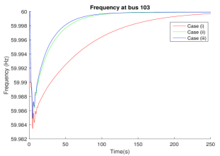
Figure 1: Frequency at bus 103 with: i) 10 generators, ii) 10 generators and 20 controllable loads, iii) 15 generators and 20 controllable loads, contributing to secondary frequency control.

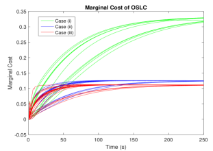
Figure 2: Marginal costs for controllable loads and generators with non-equal cost coefficients for the three test cases.

The test system consists of 93 load buses serving different types of loads including constant active and reactive loads and 47 generation buses. The overall system has a total real power of 28.55GW. For our simulation, we added three loads on units 2, 9, and 17, each having a step increase of magnitude $1$ p.u. (base 100MVA) at $t=1$ second.

Controllable demand was considered within the simulations, with loads controlled every 10ms. The disutility function for the deviation $d^{c}_{j}$ in controllable loads in each bus was $C_{dj}(d^{c}_{j})=\frac{1}{2}\alpha_{j}(d^{c}_{j})^{2}$. The selected values for cost coefficients were $\alpha_{j}=1$ for load buses $1-5$ and $11-15$ and $\alpha_{j}=2$ for the rest. Similarly, the cost functions for deviations $p^{M}_{j}$ in generation were $C_{j}(p^{M}_{j})=\frac{1}{2}\kappa_{j}(p^{M}_{j})^{2}$, where $\kappa_{j}$ were selected as the inverse of the generators droop coefficients, as suggested in (10).

Consider the static and first order dynamic schemes given by $d^{c}_{j}=(C_{dj}^{\prime})^{-1}(\omega_{j}-p^{c}_{j})$ and $\dot{d}^{c}_{j}=-d^{c}_{j}+(C_{dj}^{\prime})^{-1}(\omega_{j}-p^{c}_{j}),j\in N$, where $p^{c}_{j}$ has dynamics as described in (6). We refer to the resulting dynamics as Static and Dynamic OSLC respectively since in both cases, steady state conditions that solve the OSLC problem were used. As discussed in Section VI, in the presence of arbitrarily small frequency damping, both schemes satisfy Assumption 5 and are thus included in our framework.

The system was tested on three different cases. In case (i) 10 generators were employed to perform secondary frequency control by having frequency and power command as inputs. In case (ii) controllable loads were included on 20 load buses in addition to the 10 generators. Controllable load dynamics in 10 buses were described by Static OSLC and in the rest by Dynamic OSLC. Finally, in case (iii), all controllable loads of case (ii) and 15 generators where used for secondary frequency control. Note that the 15 generators used for secondary frequency control had third, fourth and fifth order turbine governor dynamics.

The frequency at bus 103 for the three tested cases is shown in Fig. 1. From this figure, we observe that in all cases the frequency returns to its nominal value. However, the presence of controllable loads makes the frequency return much faster and with a smaller overshoot.

Furthermore, from Fig. 2, it is observed that the marginal costs at all controlled loads and generators that contribute to secondary frequency control, converge to the same value. This illustrates the optimality in the power allocation among generators and loads, since equality in the marginal cost is necessary to solve (7) when the power generated does not saturate to its maximum/minimum value.

VIII Conclusion

We have considered the problem of designing distributed schemes for secondary frequency control such that stability and optimality of the power allocation can be guaranteed. In particular, we have considered general classes of generation and demand control dynamics and have shown that a dissipativity condition in conjunction with appropriate decentralized conditions on their steady state behavior can provide such stability and optimality guarantees. We have also discussed that for linear systems the dissipativity condition can be easily verified by solving a corresponding LMI and shown that the requirement to have knowledge of demand may be relaxed by incorporating an appropriate observer. Our results have been illustrated with simulations on the NPCC 140-bus system. Interesting potential extensions in the analysis include incorporating voltage dynamics, more advanced communication structures, as well as more advanced models for the loads where their switching behavior is taken into account.

Appendix A

In this appendix we prove our main results, Theorems  1 - 2, and also Lemmas 1-2, Theorem 3 and Proposition 1.

Throughout the proofs we will make use of the following equilibrium equations for the dynamics in (3)–(4),

$$0=\omega^{*}_{i}-\omega^{*}_{j},\;(i,j)\in E,$$ (17a)

$$0=-p_{j}^{L}+p_{j}^{M,*}-(d^{c,*}_{j}+d^{u,*}_{j})-\sum_{k:j\rightarrow k}p^{*}_{jk}+\sum_{i:i\rightarrow j}p^{*}_{ij},\;j\in G,$$ (17b)

$$0=-p_{j}^{L}-(d^{c,*}_{j}+d^{u,*}_{j})-\sum_{k:j\rightarrow k}p^{*}_{jk}+\sum_{i:i\rightarrow j}p^{*}_{ij},\;j\in L,$$ (17c)

$$p^{M,*}_{j}=k_{p^{M}_{j}}(\zeta_{j}^{*}),\;j\in G,$$ (17d)

$${\color[rgb]{0,0,0}d^{c,*}_{j}=k_{d^{c}_{j}}(\zeta_{j}^{*}),\quad\zeta_{j}^{\ast}=[-\omega_{j}^{*}\;p_{j}^{c,*}]^{T},\quad j\in N.}$$ (17e)

Proof of Lemma 1: In order to show that $\omega^{*}=\boldsymbol{0}_{|N|}$, we sum equations (6b) at equilibrium for all $j\in N$, resulting in $\sum\limits_{j\in N}s^{*}_{j}=\sum\limits_{j\in N}p^{L}_{j}$, which shows that $\sum\limits_{j\in N}d^{u,*}_{j}=0$ (by summing (17b) and (17c) over all $j\in G$ and $j\in L$ respectively). Then, Assumption 3 implies that this equality holds only if $\omega^{*}=\boldsymbol{0}_{|N|}$. ∎

Proof of Theorem 1: Due to Assumption 1, $C_{j}^{\prime}$ and $C_{dj}^{\prime}$ are strictly increasing and hence invertible. Therefore all variables in (10) are well-defined. Also, Assumption 1 guarantees that the OSLC optimization problem (7) is convex and has a continuously differentiable cost function. Thus, a point $(\bar{p}^{M},\bar{d}^{c})$ is a global minimum for (7) if and only if it satisfies the KKT conditions [28]

$$C_{j}^{\prime}(\bar{p}^{M}_{j})=\nu-\lambda_{j}^{+}+\lambda_{j}^{-},\;j\in G,$$ (18a)

$$C_{dj}^{\prime}(\bar{d}^{c}_{j})=-\nu-\mu_{j}^{+}+\mu_{j}^{-},\;j\in N,$$ (18b)

$$\sum\limits_{j\in G}\bar{p}_{j}^{M}=\sum\limits_{j\in N}(\bar{d}^{c}_{j}+p_{j}^{L}),$$ (18c)

$$p^{M,min}_{j}\leq\bar{p}^{M}_{j}\leq p^{M,max}_{j},\;j\in G,$$ (18d)

$$d^{c,min}_{j}\leq\bar{d}^{c}_{j}\leq d^{c,max}_{j},\;j\in N,$$ (18e)

$$\lambda_{j}^{+}(\bar{p}^{M}_{j}-p^{M,max}_{j})=0,\;\lambda_{j}^{-}(\bar{p}^{M}_{j}-p^{M,min}_{j})=0,\;j\in G,$$ (18f)

$$\mu^{+}(\bar{d}^{c}_{j}-d^{c,max}_{j})=0,\;\mu^{-}(\bar{d}^{c}_{j}-d^{c,min}_{j})=0,\;j\in{\color[rgb]{0,0,0}N},$$ (18g)

for some constants $\nu\in\mathbb{R}$ and $\lambda_{j}^{+},\lambda_{j}^{-},\mu_{j}^{+},\mu_{j}^{-}\geq 0$. It will be shown below that these conditions are satisfied by the equilibrium values $(\bar{p}^{M},\bar{d}^{c})=(p^{M,*},d^{c,*})$ defined by equations (17d),  (17e) and (10).

Since $C_{j}^{\prime}$ and $C_{dj}^{\prime}$ are strictly increasing, we can uniquely define $\beta_{j}^{M,max}\!\!:=\!\!C_{j}^{\prime}(p^{M,max}_{j})$, $\beta_{j}^{M,min}\!\!:=\!\!C_{j}^{\prime}(p^{M,min}_{j})$, $\beta_{j}^{c,max}\!\!:=-C_{dj}^{\prime}(d^{c,max}_{j})$, and $\beta_{j}^{c,min}\!\!:=-C_{dj}^{\prime}(d^{c,min}_{j})$. We let $\beta^{*}_{0}=f(\zeta^{*}_{j})$ where $f(.)$ is the function in the theorem statement. Note that function $f$ is common at every bus and is surjective hence $\forall\beta^{*}_{0}\in\mathbb{R},\exists\zeta$ such that $f(\zeta)=\beta^{*}_{0}$. Also note that the $\zeta_{j}$ are equal $\forall j$ at equilibrium, therefore $\beta^{*}_{0}$ is the same at each bus $j$. We now define in terms of these quantities the nonnegative constants

$$\lambda_{j}^{+}:=(\beta^{*}_{0}-\beta^{M,max}_{j})\,\mathds{1}_{(\beta^{*}_{0}\geq\beta^{M,max}_{j})},$$

$$\lambda_{j}^{-}:=(\beta^{M,min}_{j}-\beta^{*}_{0})\,\mathds{1}_{(\beta^{*}_{0}\leq\beta^{M,min}_{j})},$$

$$\mu_{j}^{+}:=(\beta^{c,max}_{j}-\beta^{*}_{0})\,\mathds{1}_{(\beta^{*}_{0}\leq\beta^{c,max}_{j})},$$

$$\mu_{j}^{-}:=(\beta^{*}_{0}-\beta^{c,min}_{j})\,\mathds{1}_{(\beta^{*}_{0}\geq\beta^{c,min}_{j})}.$$

Then, since $(C_{j}^{\prime})^{-1}(\beta_{0}^{*})\geq p^{M,max}_{j}\Leftrightarrow\beta^{*}_{0}\geq\beta^{M,max}_{j}$, $(C_{j}^{\prime})^{-1}(\beta_{0}^{*})\leq p^{M,min}_{j}\Leftrightarrow\beta^{*}_{0}\leq\beta^{M,min}_{j}$, $(C_{dj}^{\prime})^{-1}(-\beta_{0}^{*})\geq d^{c,max}_{j}\Leftrightarrow\beta^{*}_{0}\leq\beta^{c,max}_{j}$, and $(C_{dj}^{\prime})^{-1}(-\beta_{0}^{*})\leq d^{c,min}_{j}\Leftrightarrow\beta^{*}_{0}\geq\beta^{c,min}_{j}$, it follows by (17d), (17e), and (10) that the complementary slackness conditions (18f) and (18g) are satisfied.

Now define $\nu=\beta_{0}^{*}$. Then $(C_{j}^{\prime})^{-1}(\nu-\lambda_{j}^{+}+\lambda_{j}^{-})=(C_{j}^{\prime})^{-1}\Big{(}[\beta_{0}^{*}]_{\beta^{M,min}_{j}}^{\beta^{M,max}_{j}}\Big{)}=[(C_{j}^{\prime})^{-1}(\beta_{0}^{*})]_{p^{M,min}_{j}}^{p^{M,max}_{j}}=p^{M,*}_{j}$, by the above definitions and equations (17d) and (10). Thus, the optimality condition (18a) holds. Analogously, $(C_{dj}^{\prime})^{-1}(-\nu-\mu^{+}+\mu^{-})=(C_{dj}^{\prime})^{-1}\Big{(}[-\beta_{0}^{*}]_{-\beta^{c,min}_{j}}^{-\beta^{c,max}_{j}}\Big{)}=[(C_{dj}^{\prime})^{-1}(-\beta_{0}^{*})]_{d^{c,min}_{j}}^{d^{c,max}_{j}}=d^{c,*}_{j}$, by (17e) and (10), satisfying (18b).

Summing equations  (17b) and (17c) over all $j\in G$ and $j\in L$ respectively and using the fact that $\sum_{j\in N}d^{u,*}_{j}=0$ as shown in the proof of Lemma 1 shows that (18c) holds. Finally, the saturation constraints in (10) verify (18d) and (18e).

Hence, the values $(\bar{p}^{M},\bar{d}^{c})=(p^{M,*},d^{c,*})$ satisfy the KKT conditions (18). Therefore, the equilibrium values $p^{M,*}$ and $d^{c,*}$ define a global minimum for (7). ∎

Proof of Theorem 2: We will use the dynamics in (3)–(6) and the conditions of Assumption 5 to define a Lyapunov function for the system (3)–(6).

Firstly, let $V_{F}(\omega^{G})=\frac{1}{2}\sum_{j\in G}M_{j}(\omega_{j}-\omega^{*}_{j})^{2}$. The time-derivative of $V_{F}$ along the trajectories of (3)–(4) is given by

$$\dot{V}_{F} =\sum_{j\in N}(\omega_{j}-\omega^{*}_{j})\Bigg{(}-p^{L}_{j}+s_{j}-d^{u}_{j}-\sum_{k:j\rightarrow k}p_{jk}+\sum_{i:i\rightarrow j}p_{ij}\Bigg{)},$$

by substituting (3b) for $\dot{\omega}_{j}$ for $j\in G$ and adding extra terms for $j\in L$, which are equal to zero by (3c). Subtracting the product of $(\omega_{j}-\omega^{*}_{j})$ with each term in (17b) and (17c), this becomes

$$\dot{V}_{F}= \sum_{j\in N}\Bigg{(}{\color[rgb]{0,0,0}(\omega_{j}}-\omega^{*}_{j})(s_{j}-s^{*}_{j})+(\omega_{j}-\omega^{*}_{j})(-d^{u}_{j}-(-d^{u,*}_{j}))\Bigg{)}$$

$${\color[rgb]{0,0,0}+\sum_{(i,j)\in E}}(p_{ij}-p^{*}_{ij})(\omega_{j}-\omega_{i}),$$ (19)

using the equilibrium condition (17a) for the final term.

Furthermore, let $V_{C}(p^{c})=\frac{1}{2}\sum_{j\in N}\gamma_{j}(p^{c}_{j}-p^{c,*}_{j})^{2}$. Using (6b) the time derivative of $V_{C}$ can be written as

$$\dot{V}_{C}=\sum_{j\in N}(p^{c}_{j}-p^{c,*}_{j})\Big{(}(-s_{j}+s^{*}_{j})\\ -\sum_{k:j\rightarrow k}(\psi_{jk}-\psi^{*}_{jk})+\sum_{i:i\rightarrow j}(\psi_{ij}-\psi^{*}_{ij})\Big{)}.$$ (20)

Additionally, define $V_{P}(\eta)=\sum_{(i,j)\in E}B_{ij}\int_{\eta^{*}_{ij}}^{\eta_{ij}}(\sin\theta-{\color[rgb]{0,0,0}\sin\eta^{*}_{ij}})\,d\theta$. Using (3a) and (3d), the time-derivative is given by

$$\dot{V}_{P} =\sum_{(i,j)\in E}B_{ij}(\sin\eta_{ij}-\sin\eta^{*}_{ij})(\omega_{i}-\omega_{j})$$

$$=\sum_{(i,j)\in E}(p_{ij}-p^{*}_{ij})(\omega_{i}-\omega_{j}).$$ (21)

Finally, consider $V_{\psi}(\psi)=\frac{1}{2}\sum_{(i,j)\in{\color[rgb]{0,0,0}\tilde{E}}}\gamma_{ij}(\psi_{ij}-\psi^{*}_{ij})^{2}$ with time derivative given by (6a) as

$$\dot{V}_{\psi}=\sum_{(i,j)\in{\color[rgb]{0,0,0}\tilde{E}}}(\psi_{ij}-\psi^{*}_{ij})((p^{c}_{i}-p^{c,*}_{i})-(p^{c}_{j}-p^{c,*}_{j})).$$ (22)

Furthermore, from the dissipativity condition in Assumption 5 the following holds: There exist open neighborhoods $U_{j}$ of $\omega^{*}_{j}$ and $U^{c}_{j}$ of $p^{c,*}_{j}$ for each $j\in N$, open neighborhoods $X^{G}_{j}$ of $(x^{M,j,*},x^{c,j,*},x^{u,j,*})$ and $X^{L}_{j}$ of $(x^{c,j,*},x^{u,j,*})$ for each $j\in G$ and $j\in L$ respectively, and continuously differentiable, positive semidefinite functions $V^{D}_{j}(x^{M,j},x^{c,j},x^{u,j}),j\in G$ and $V^{D}_{j}(x^{c,j},x^{u,j}),j\in L$, satisfying (8) with supply rate given by (9), i.e.,

$$\dot{V}^{D}_{j}\leq[(s_{j}-s^{*}_{j})\;\;\;(-d^{u}_{j}-(-d^{u,*}_{j}))]\begin{bmatrix}1&1\\ 1&0\end{bmatrix}(\zeta_{j}-\zeta^{*}_{j})\\ {\color[rgb]{0,0,0}-{\color[rgb]{0,0,0}\phi_{j}}(\zeta_{j}-\zeta^{*}_{j}),}\hskip 8.53581ptj\in N,$$ (23)

for all $\omega_{j}\in U_{j}$, $p^{c}_{j}$ in $U^{c}_{j}$ for $j\in N$ and all $(x^{M,j},x^{c,j},x^{u,j})\in X^{G}_{j}$ and $(x^{c,j},x^{u,j})\in X^{L}_{j}$ for $j\in G$ and $j\in L$ respectively.

Based on the above, we define the function

$$V(\eta,\psi,\omega^{G},x^{M},x^{c},x^{u},p^{c})=V_{F}+V_{P}+\sum_{j\in N}V^{D}_{j}+V_{C}+V_{\psi}$$ (24)

which we aim to use in Lasalle’s theorem. Using (19) - (22), the time derivative of V is given by

$$\dot{V}= \sum_{j\in N}\bigl{[}(\omega_{j}-\omega^{*}_{j})(s_{j}-s^{*}_{j})+\dot{V}^{D}_{j}+(p^{c}_{j}-p^{c,*}_{j})(-s_{j}+s^{*}_{j})$$

$$\hskip 71.13188pt+(\omega_{j}-\omega^{*}_{j})(-d^{u}_{j}-(-d^{u,*}_{j})\bigr{]}.$$ (25)

Using (23) it therefore holds that

$$\dot{V} \leq\sum_{j\in N}\Big{(}-{\color[rgb]{0,0,0}\phi_{j}}(\zeta_{j}-{\color[rgb]{0,0,0}\zeta^{*}_{j})}\Big{)}\leq 0$$ (26)

whenever $\omega_{j}\in U_{j}$, $p^{c}_{j}\in{\color[rgb]{0,0,0}U^{c}_{j}}$ for $j\in N$, $(x^{M,j},x^{c,j},x^{u,j})\in X^{G}_{j}$ for $j\in G$, and $(x^{c,j},x^{u,j})\in X^{L}_{j}$ for $j\in L$.

Clearly $V_{F}$ has a strict global minimum at $\omega^{G,*}$ and $V^{D}_{j}$ has strict local minima at $(x^{M,j,*},x^{c,j,*},x^{u,j,*})$ and $(x^{c,j,*},x^{u,j,*})$ for $j\in G$ and $j\in L$ respectively by Assumption 5 and Definition 2. Furthermore, $V_{C}$ and $V_{\psi}$ have strict global minima at $p^{c,*}$ and $\psi^{*}$ respectively. Furthermore, Assumption 2 guarantees the existence of some neighborhood of each $\eta^{*}_{ij}$ in which $V_{P}$ is increasing. Since the integrand is zero at the lower limit of the integration, $\eta^{*}_{ij}$, this immediately implies that $V_{P}$ has a strict local minimum at $\eta^{*}$. Thus, $V$ has a strict local minimum at the point $Q^{*}:=(\eta^{*},\psi^{*},\omega^{G,*},x^{M,*},x^{c,*},x^{u,*}$, $p^{c,*})$. From Assumption 4, we know that, provided $(\eta,\omega^{G},x^{c},x^{u},p^{c})\in T$, $\omega^{L}$ can be uniquely determined from these quantities. Therefore, the states of the differential equation system (3)–(6) with $(\eta,\omega^{G},x^{c},x^{u},p^{c})$ within the region $T$ can be expressed as $(\eta,\psi,\omega^{G},x^{M},x^{c},x^{u},p^{c})$. We now choose a neighborhood in the coordinates $(\eta,\psi,\omega^{G},x^{M},x^{c},x^{u},p^{c})$ about $Q^{*}$ on which the following hold:

1. $Q^{*}$ is a strict minimum of $V$,

2. $(\eta,\omega^{G},x^{c},x^{u},p^{c})\in T$,

3. $\omega_{j}\in U_{j}$, $p^{c}_{j}\in{\color[rgb]{0,0,0}U^{c}_{j}}$ for $j\in N$, and $(x^{M,j},x^{c,j},x^{u,j})\in X^{G}_{j}$, $(x^{c,j},x^{u,j})\in X^{L}_{j}$ for $j\in G$, $j\in L$ respectively,

4. $x^{M,j}$, $x^{c,j}$, and $x^{u,j}$ all lie within their respective neighborhoods $X_{0}$ as defined in Section III-A.

Recalling now (26), it is easy to see that within this neighborhood, $V$ is a nonincreasing function of all the system states and has a strict local minimum at $Q^{*}$. Consequently, the connected component of the level set $\{(\eta,\psi,\omega^{G},x^{M},x^{c},x^{u},p^{c})\colon V\leq\epsilon\}$ containing $Q^{*}$ is guaranteed to be both compact and positively invariant with respect to the system (3)–(6) for sufficiently small $\epsilon>0$. Therefore, there exists a compact positively invariant set $\Xi$ for (3)–(6) containing $Q^{*}$.

Lasalle’s Invariance Principle can now be applied with the function $V$ on the compact positively invariant set $\Xi$. This guarantees that all solutions of (3)–(6) with initial conditions $(\eta(0),\psi(0),\omega^{G}(0),x^{M}(0),x^{c}(0),x^{u}(0),p^{c}(0))\in\Xi$ converge to the largest invariant set within $\Xi\,\cap\,\{(\eta,\psi,\omega^{G},x^{M},x^{c},x^{u},p^{c})\colon\dot{V}=0\}$. We now consider this invariant set. If $\dot{V}=0$ holds at a point within $\Xi$, then (26) holds with equality, hence we must have $\omega=\omega^{*}$ and $p^{c}_{j}=p^{c,*}_{j}$ at all buses $j$ where Assumption 5(a) holds. The fact that $\omega$ is constant guarantees from (3a), (3d) that $\eta$ and $p$ are also constant. This is sufficient to deduce from (3b)–(3c) that $s$ is also constant. If instead Assumption 5(b) holds at a bus $j$ we have that $\omega=\omega^{*}$ when $\dot{V}=0$. Furthermore, we have the additional property that if $\omega_{j}$ and $s_{j}$ are constant then $p^{c}_{j}$ cannot be a sinusoid. This latter property guarantees that $p^{c}_{j}$ is also constant by noting that the dynamics for the power command (6) with constant $s_{j}$, allow $p^{c}_{j}$ to be either a constant or a sinusoid within a compact invariant set. Hence, we have $\omega=\omega^{*}$ and $p^{c}=p^{c,*}$ in the invariant set considered.

Furthermore, note that $\omega=\omega^{*}$, $p^{c}=p^{c,*}$ within the invariant set implies by the definitions in Section II that $(x^{M},x^{c},x^{u})$ converge to the point $(x^{M,*},x^{c,*},x^{u,*})$, at which $V^{D}_{j}$ take strict local minima from Assumption 5. Thus, from  (23) and (Appendix A) it follows that the values of $V^{D}_{j}$ must decrease along all nontrivial trajectories within the invariant set, contradicting $\dot{V}^{D}_{j}=0$. The fact that $(p^{c},s)=(p^{c,*},s^{*}$) is sufficient to show that $\psi$ equals some constant $\psi^{*}$. Using the same argument, it can be shown that within the invariant set, the fact that $\zeta=\zeta^{*}$ implies that $(x^{M},x^{c},x^{u},p^{M},d^{c},d^{u})$ converges to $(x^{M,*},x^{c,*},x^{u,*},p^{M,*},d^{c,*},d^{u,*})$. Therefore, we conclude by Lasalle’s Invariance Principle that all solutions of (3)–(6) with initial conditions $(\eta(0),\psi(0),\omega^{G}(0),x^{M}(0),x^{c}(0),x^{u}(0),p^{c}(0))\in\Xi$ converge to the set of equilibrium points as defined in Definition 1. Finally, choosing for $S$ any open neighborhood of $Q^{*}$ within $\Xi$ completes the proof for convergence. From Lemma 1 it can then be deduced that $\omega^{*}=\boldsymbol{0}_{|N|}$. Furthermore, noting that all conditions of Theorem 1 hold shows the convergence to an optimal solution of the OSLC problem (7). ∎

Remark 9

It should be noted that for given $p^{c,*}$ and $\omega^{*}$ all $(\eta^{*},x^{M,*},x^{c,*},x^{u,*})$ are unique. The uniqueness of $\eta^{*}$ can be seen by noting that $\eta_{ij}=\theta_{i}-\theta_{j},(i,j)\in E$, which requires $\eta$ to lie in a space where a corresponding vector $\theta$ exists. Furthermore, the value of $p^{c,*}$ becomes unique when (10) holds. This follows from summing (17b)–(17c) over all buses and noting that the strict convexity of the cost functions and the monotonicity of $f$ in (10) makes the static input output maps from $p^{c,*}$ to $s^{*}$ monotonically increasing. The values of $\psi^{*}$ are non-unique for general network topologies.

Proof of Theorem 3: The proof follows from the fact that the function $V^{B}_{j}$ defined as

$$V^{B}_{j}=\frac{1}{2}M_{j}(\omega_{j}-\omega^{*}_{j})^{2}+\frac{1}{2}\gamma_{j}(p^{c}_{j}-p^{c,*}_{j})^{2}+V^{D}_{j},$$ (27)

where $V^{D}_{j}$ is as in (23) with $\phi_{j}=0$, is a storage function for the system $B_{j}$. In particular, using arguments similar to those in the proof of Theorem 2, it can be shown that

$$\dot{V}^{B}_{j}\leq(p^{c}_{j}-p^{c,*}_{j})\biggl{(}\sum_{i:i\rightarrow j}(\psi_{ij}-\psi_{ij}^{\ast})-\sum_{k:j\rightarrow k}(\psi_{jk}-\psi_{jk}^{\ast})\biggr{)}\\ +(-\omega_{j}-(-\omega^{*}_{j}))\biggl{(}\sum_{k:j\rightarrow k}(p_{jk}-p_{jk}^{\ast})-\sum_{i:i\rightarrow j}(p_{ij}-p_{ij}^{\ast})\biggr{)}$$ (28)

and therefore that system $B_{j}$ is passive. ∎

Proof of Lemma 2: Using (16d) at equilibrium, it can be deduced that $\chi^{*}_{j}=s^{*}_{j}-d^{u,*}_{j}-\sum_{k:j\rightarrow k}p^{*}_{jk}+\sum_{i:i\rightarrow j}p^{*}_{ij}$. Hence, it follows by summing (16b) at equilibrium over all buses that $\sum\limits_{j\in N}s^{*}_{j}=\sum\limits_{j\in N}\chi^{*}_{j}=\sum\limits_{j\in N}s^{*}_{j}-d^{u,*}_{j}$, which results to $\sum\limits_{j\in N}d^{u,*}_{j}=0$. Hence, from Assumption 3, it follows that $\omega^{*}=\boldsymbol{0}_{|N|}$. ∎

Proof of Proposition 1: We shall make use of the Lyapunov function in (24) to construct a new Lyapunov function for the system (3) – (5), (16).

First, consider the function

$$V_{b}(b,\chi,\omega)=\frac{1}{2}\sum_{j\in G}\big{(}M_{j}((b_{j}-b^{*}_{j})-(\omega_{j}-\omega^{*}_{j}))^{2}\\ +\tau_{\chi,j}(\chi_{j}-\chi^{*}_{j})^{2}\big{)},$$ (29)

and note that its time-derivative along the trajectories of (16) is given by

$$\dot{V}_{b}=\sum_{j\in N}\biggr{(}-(\chi_{j}-\chi^{*}_{j})[(p^{c}_{j}-p^{c,*}_{j})+(\chi_{j}-\chi^{*}_{j})]\biggr{)},$$ (30)

noting that for $j\in L$ it holds that $\chi=\chi^{*}$, and hence the added terms in (30) are equal to zero.

Furthermore, the time-derivative of $V_{C}(p^{c})=\frac{1}{2}\sum_{j\in N}\gamma_{j}(p^{c}_{j}-p^{c,*}_{j})^{2}$ under (16b) is given by

$$\dot{V}_{C}=\sum_{j\in N}(p^{c}_{j}-p^{c,*}_{j})\Big{(}(-s_{j}+s^{*}_{j})+(\chi_{j}-\chi^{*}_{j})\\ -\sum_{k:j\rightarrow k}(\psi_{jk}-\psi^{*}_{jk})+\sum_{i:i\rightarrow j}(\psi_{ij}-\psi^{*}_{ij})\Big{)}.$$ (31)

Now consider the function $V$ in (24) and note that its derivative is as in (Appendix A) with an extra term given by $\sum_{j\in N}(p^{c}_{j}-p^{c,*}_{j})(\chi_{j}-\chi^{*}_{j})$. Then consider the function

$$V_{O}(\eta,\psi,\omega^{G},x^{M},x^{c},x^{u},p^{c},b,\chi)=V+V_{b}$$ (32)

which can be shown to have a time derivative given by

$$\dot{V}_{O} \leq\sum_{j\in N}\Big{(}-\phi_{j}(\zeta_{j}-\zeta^{*}_{j})-(\chi_{j}-\chi^{*}_{j})^{2}\Big{)}\leq 0,$$ (33)

by similar arguments as in the proof of Theorem 2.

Now, in analogy to the proof of Theorem 2, it can be shown that an invariant compact set $\Xi_{O}$ exists such that $\{(\eta,\psi,\omega^{G},x^{M},x^{c},x^{u},p^{c},b,\chi)\colon V_{O}\leq\epsilon\}$. Then, Lasalle’s theorem can be invoked to show that all solutions of (3) – (5), (16) with initial conditions within $\Xi_{O}$ will converge to the largest invariant set within $\Xi_{O}\,\cap\,\{(\eta,\psi,\omega^{G},x^{M},x^{c},x^{u},p^{c},b,\chi)\colon\dot{V}=0\}$. Within this invariant set, it holds that $(\omega,\chi)=(\omega^{*},\chi^{*})$. Applying the same arguments as in the proof of Theorem 2 shows that $(\eta,\psi,x^{M},x^{c},x^{u},p^{M},d^{c},d^{u},p^{c})$ converges to $(\eta^{*},\psi^{*},x^{M,*},x^{c,*},x^{u,*},p^{M,*},d^{c,*},d^{u,*},p^{c,*})$ which implies the convergence of $b$ to $b^{*}$ from the dynamics in (16d). The optimality result follows directly from the proof of Theorem 1 since none of its arguments are affected from the dynamics in (16). ∎

Appendix B

In this appendix we show that Assumption 5 is a necessary and sufficient condition for the passivity of bus systems $B_{j}$, described in Section VI-A, when their dynamics are affine nonlinear, i.e. are characterized by the following state space representation:

$$\dot{x}=f(x)+g(x)u,$$

$$y=h(x).$$ (34)

For the proof, we shall make use of Lemma 3 below. Within it, we shall consider the negative feedback interconnection of

$$\Sigma_{1}:\begin{cases}\dot{x}_{1}=u_{1}\\ y_{1}=h_{1}(x_{1})\end{cases},\Sigma_{2}:\begin{cases}\dot{x}_{2}=f_{2}(x_{2})+g_{2}(x_{2})u_{2}\\ y_{2}=h_{2}(x_{2})+k_{2}(u_{2})\end{cases}$$ (35)

such that $u_{2}=y_{1}$ and $u_{1}=r-y_{2}$, where $r(t)\in\mathbb{R}^{n}$ is some reference input applied to the closed-loop system, $x_{1}(t)\in\mathbb{R}^{n},x_{2}(t)\in\mathbb{R}^{n_{2}}$ and $y_{1}(t),y_{2}(t)\in\mathbb{R}^{n}$ are the states and outputs of $\Sigma_{1}$ and $\Sigma_{2}$ respectively and $h_{1},k_{2}:\mathbb{R}^{n}\rightarrow\mathbb{R}^{n}$, and $f_{2},g_{2},h_{2}:\mathbb{R}^{n_{2}}\rightarrow\mathbb{R}^{n}$ are functions describing the dynamics of $\Sigma_{1}$ and $\Sigma_{2}$. The closed-loop system, denoted by $\Sigma$, writes as

$$\Sigma:\begin{cases}\dot{x}_{1}&=-h_{2}(x_{2})-k_{2}(h_{1}(x_{1}))+r,\\ \dot{x}_{2}&=f_{2}(x_{2})+g_{2}(x_{2})h_{1}(x_{1}),\\ y_{1}&=h_{1}(x_{1}).\end{cases}$$ (36)

Without loss of generality we also assume in the lemma below that $h_{1}(0),k_{2}(0),f_{2}(0),h_{2}(0)$ are equal to zero and the passivity properties stated are considered about this equilibrium point.

Lemma 3

Consider the negative feedback interconnection $\Sigma$ described by (36) of two subsystems $\Sigma_{1}$ and $\Sigma_{2}$ described by (35). Assume that $\Sigma$ is passive from $r$ to $y_{1}$, and $\Sigma_{1}$ is passive from $u_{1}$ to $y_{1}$. Then, $\Sigma_{2}$ is passive from $u_{2}$ to $y_{2}$.

Proof of Lemma 3: From the passivity of $\Sigma$ and [29, Corollary 4.1.5] there exists a positive definite continuously differentiable storage function $V(x_{1},x_{2})$, defined with respect to an equilibrium, such that

$$-\frac{\partial{V}}{\partial{x_{1}}}(x_{1},x_{2})h_{2}(x_{2})-\frac{\partial{V}}{\partial{x_{1}}}(x_{1},x_{2})k_{2}(h_{1}(x_{1}))$$

$$+\frac{\partial{V}}{\partial{x_{2}}}(x_{1},x_{2})f_{2}(x_{2})+\frac{\partial{V}}{\partial{x_{2}}}(x_{1},x_{2})g_{2}(x_{2})h_{1}(x_{1})\leq 0$$ (37)

and

$$\frac{\partial{V}}{\partial{x_{1}}}(x_{1},x_{2})=h_{1}^{T}(x_{1}).$$

Similarly, from the passivity of $\Sigma_{1}$ and [29, Corollary 4.1.5] there exists a positive definite continuously differentiable storage function $V_{1}$ such that

$$\frac{\partial{V_{1}}}{\partial{x_{1}}}(x_{1})=h_{1}^{T}(x_{1}).$$ (38)

Hence,

$$\frac{\partial{V}}{\partial{x_{1}}}(x_{1},x_{2})=\frac{\partial{V_{1}}}{\partial{x_{1}}}(x_{1}).$$ (39)

Substituting this back to (Appendix B) yields

$$\frac{\partial{V}}{\partial{x_{2}}} (x_{1},x_{2})f_{2}(x_{2})+\frac{\partial{V}}{\partial{x_{2}}}(x_{1},x_{2})g_{2}(x_{2})h_{1}(x_{1})$$

$$\leq\frac{\partial{V_{1}}}{\partial{x_{1}}}(x_{1})(h_{2}(x_{2})+k_{2}(h_{1}(x_{1}))$$

$$=h_{1}^{T}(x_{1})(h_{2}(x_{2})+k_{2}(h_{1}(x_{1})),$$ (40)

where the last inequality follows from (38). Now let $V$ be written as

$$V(x_{1},x_{2})=V_{1}(x_{1})+V_{2}(x_{2})$$ (41)

for some continuously differentiable $V_{2}$. The fact that $V_{2}$ is only a function of $x_{2}$ descends from (39). Also note that $V_{2}(x_{2})$ is positive definite. By substituting the above into (Appendix B), we conclude that

$$\frac{\partial{V_{2}}}{\partial{x_{2}}}(x_{2})f_{2}(x_{2})+\frac{\partial{V_{2}}}{\partial{x_{2}}}(x_{2})g_{2}(x_{2})u_{2}\leq u^{T}_{2}y_{2}$$

which implies the passivity of $\Sigma_{2}$. ∎

The following lemma shows that Assumption 5 is a necessary and sufficient condition for the passivity of generation bus system $B_{j}$. Note that the extension to load buses is trivial and thus omitted.

Lemma 4

Consider the system described by (3) - (6) and its representation by systems $I$ and $B$, defined in section VI-A and let the dynamics for $B_{j}$ be described by (36). Then, the dissipativity condition in Assumption 5 with $\phi=0$ is necessary and sufficient for the passivity of subsystems $B_{j},j\in G$ about the equilibrium point considered in Assumption 5.

Proof of Lemma 4: The proof for the necessity of the condition follows from Lemma 3 when the following substitutions are made

$$r=\begin{bmatrix}\sum_{k:j\rightarrow k}(p_{jk}-p^{*}_{jk})-\sum_{i:i\rightarrow j}(p_{ij}-p^{*}_{ij})\\ \sum_{i:i\rightarrow j}(\psi_{ij}-\psi^{*}_{ij})-\sum_{k:j\rightarrow k}(\psi_{jk}-\psi^{*}_{jk})\end{bmatrix},$$

$$y_{1}=\begin{bmatrix}-(\omega_{j}-\omega^{*}_{j})\\ p^{c}_{j}-p^{c,*}_{j}\end{bmatrix},\;y_{2}=\begin{bmatrix}(s_{j}-s_{j}^{\ast})-(d^{u}_{j}-d^{u,\ast}_{j})\\ (s_{j}-s_{j}^{\ast})\end{bmatrix}.$$

The sufficiency proof follows directly from Theorem 3. ∎

References

• [1] H. Lund, “Large-scale integration of optimal combinations of PV, wind and wave power into the electricity supply,” Renewable Energy, vol. 31, no. 4, pp. 503–515, 2006.
• [2] A. Ipakchi, and F. Albuyeh, “Grid of the future,” IEEE Power and Energy Magazine, vol. 7, no. 2, pp. 52–62, March 2009.
• [3] A. Molina-Garciá, F. Bouffard, and D. S. Kirschen, “Decentralized demand-side contribution to primary frequency control,” IEEE Trans. Power Syst., vol. 26, no. 1, pp. 411–419, May 2010.
• [4] S. Trip, and C. De Persis. “Optimal generation in structure-preserving power networks with second-order turbine-governor dynamics,” European Control Conference (ECC), 2016.
• [5] A. Kasis, E. Devane, C. Spanias and I. Lestas, “Primary frequency regulation with load-side participation Part I: stability and optimality,” IEEE Transactions on Power Systems, 2016.
• [6] E. Mallada, C. Zhao, and S. Low, “Optimal load-side control for frequency regulation in smart grids,” 52nd Annual Allerton Conference on Communication, Control, and Computing, pp. 731-738, 2014.
• [7] S. Trip, M. Burger, and C. De Persis,“An internal model approach to frequency regulation in inverter-based microgrids with time-varying voltages,” IEEE 53rd Annual Conference on Decision and Control, pp. 223-228, 2014.
• [8] C. Zhao, U. Topcu, N. Li, and S. Low, “Design and stability of load-side primary frequency control in power systems,” IEEE Trans. Autom. Control, vol. 59, no. 5, pp.1177–1189, 2014.
• [9] C. Zhao, and S. Low, “Optimal decentralized primary frequency control in power networks,” IEEE 53rd Annual Conference on Decision and Control, pp 2467–2473, Dec. 2014.
• [10] E. Devane, A. Kasis, M. Antoniou, and I. Lestas, “Primary frequency regulation with load-side participation Part II: beyond passivity approaches,” IEEE Transactions on Power Systems, 2016.
• [11] Q. Shafiee, J. M. Guerrero, and J. C. Vasquez, “Distributed secondary control for islanded microgrids – a novel approach,” IEEE Trans. Power Electron., vol. 29, no. 2, pp. 1018–1031, Apr. 2013.
• [12] M. Andreasson, et al., “Distributed vs. centralized power systems frequency control,” 12th European Control Conference, pp. 3524-3529, 2013.
• [13] E. Mallada, and S. H. Low, “Distributed frequency-preserving optimal load control,” IFAC World Congress, pp. 5411-5418, 2014.
• [14] C. Zhao, E. Mallada, and S. H. Low, “Distributed generator and load-side secondary frequency control in power networks,” IEEE 49th Annual Conference on Information Sciences and Systems, pp. 1-6, 2015.
• [15] N. Li, et al., “Connecting automatic generation control and economic dispatch from an optimization view,” American Control Conference(ACC), pp. 735-740, 2014.
• [16] F. Dörfler, J. W. Simpson-Porco, and F. Bullo, “Plug-and-play control and optimization in microgrids,” 53rd IEEE Conference on Decision and Control, pp. 211-216, 2014.
• [17] J. W. Simpson-Porco, F. Dörfler, and F. Bullo, “Synchronization and power sharing for droop-controlled inverters in islanded microgrids,” Automatica, pp. 2603-2611, 2013.
• [18] F. Dörfler, J.W. Simpson-Porco, and F. Bullo, “Breaking the hierarchy: Distributed control $\&$ economic optimality in microgrids,” IEEE Trans. on control of network systems,pp. 241-253, 2016.
• [19] S. Trip, M. B rger, and C. De Persis, “An internal model approach to (optimal) frequency regulation in power grids with time-varying voltages,” Automatica, pp.240-253, 2016.
• [20] M. Andreasson, D. V. Dimarogonas, H. Sandberg, and K. H. Johansson, “Distributed PI-control with applications to power systems frequency control,” IEEE American Control Conference, pp. 3183-3188), 2014.
• [21] A. R. Bergen and V. Vittal, Power Systems Analysis. Prentice Hall, 1999.
• [22] D. J. Hill, and I. M. Mareels, “Stability theory for differential/algebraic systems with application to power systems,” IEEE Transactions on circuits and systems, pp.1416-1423, 1990.
• [23] S. Sastry, Nonlinear systems: analysis, stability and control. Springer-Verlag New York, 1999.
• [24] J.C. Willems, “Dissipative dynamical systems part I: General theory,” Archive for rational mechanics and analysis, 1972.
• [25] J.C. Willems, “Dissipative dynamical systems part II: Linear systems with quadratic supply rates,” Archive for Rational Mechanics and Analysis, 1972.
• [26] N. Monshizadeh, C. De Persis, and J. W. Simpson-Porco, “The cost of dishonesty on optimal distributed frequency control of power networks,” IEEE 55th Annual Conference on Decision and Control, 2016.
• [27] K. W. Cheung, J. Chow, and G. Rogers, Power System Toolbox, v. 3.0. Cherry Tree Scientific Software, 2009.
• [28] S. Boyd and L. Vandenberghe, Convex optimization. Cambridge University Press, 2004.
• [29] A. Van der Schaft, “L2-gain and passivity techniques in nonlinear control,” Springer Science $\&$ Business Media, 2012.
• [30] A. Kasis, E. Devane, and I. Lestas, “Stability and optimality of distributed schemes for secondary frequency regulation in power networks,” IEEE 55th Annual Conference on Decision and Control, 2016.