The Second Order Linear Model

Abstract

We study a fundamental class of regression models called the second order linear model (SLM). The SLM extends the linear model to high order functional space and has attracted considerable research interest recently. Yet how to efficiently learn the SLM under full generality using nonconvex solver still remains an open question due to several fundamental limitations of the conventional gradient descent learning framework. In this study, we try to attack this problem from a gradient-free approach which we call the moment-estimation-sequence (MES) method. We show that the conventional gradient descent heuristic is biased by the skewness of the distribution therefore is no longer the best practice of learning the SLM. Based on the MES framework, we design a nonconvex alternating iteration process to train a $d$-dimension rank-$k$ SLM within $O(kd)$ memory and one-pass of the dataset. The proposed method converges globally and linearly, achieves $\epsilon$ recovery error after retrieving $O[k^{2}d\cdot\mathrm{polylog}(kd/\epsilon)]$ samples. Furthermore, our theoretical analysis reveals that not all SLMs can be learned on every sub-gaussian distribution. When the instances are sampled from a so-called $\tau$-MIP distribution, the SLM can be learned by $O(p/\tau^{2})$ samples where $p$ and $\tau$ are positive constants depending on the skewness and kurtosis of the distribution. For non-MIP distribution, an addition diagonal-free oracle is necessary and sufficient to guarantee the learnability of the SLM. Numerical simulations verify the sharpness of our bounds on the sampling complexity and the linear convergence rate of our algorithm.

1 Introduction

The second order linear model (SLM) is a fundamental class of regression models and attracts considerable research interest recently. Given an instance $\boldsymbol{x}\in\mathbb{R}^{d}$, the SLM assumes that the label $y\in\mathbb{R}$ of $\boldsymbol{x}$ is generated by

$$y=\boldsymbol{x}{}^{\top}\boldsymbol{w}^{*}+\boldsymbol{x}{}^{\top}M^{*}\boldsymbol{x}+\xi$$ (1)

where $\{\boldsymbol{w}^{*},M^{*}\}$ are the first order and the second order coefficients respectively. The $\xi$ is an additive sub-gaussian noise term. The SLM defined in Eq. (1) covers several important models in machine learning and signal processing problems. When $\boldsymbol{w}^{*}=0$ and $M^{*}$ is a rank-one symmetric matrix, Eq. (1) is known as the phase retrieval problem (Candes et al., 2013). While $M^{*}$ is a rank-$k$ symmetric matrix, Eq. (1) is equal to the symmetric rank-one matrix sensing problem (Kueng et al., 2017; Cai and Zhang, 2015; yurtsever_sketchy_2017). For $\boldsymbol{w}^{*}\not=\boldsymbol{0}$ and $M_{i,j}^{*}=v_{i}v_{j}$ at $i\not=j$ otherwise $M_{i,i}^{*}=0$, Eq. (1) is called the Factorization Machine (FM) (Rendle, 2010). When $M_{i,i}^{*}$ is allowed to be non-zero, the model is called the Generalized Factorization Machine (gFM) (Ming Lin and Jieping Ye, 2016) . It is possible to further extend the SLM to high order functional space which leads to the Polynomial Network model (Blondel et al., 2016). lin_multi-task_2016 employ the SLM to capture the feature interaction in multi-task learning.

Although the SLM have been applied in various learning problems, there is rare research of SLM under a general setting in form of Eq. (1). A naive analysis directly following the sampling complexity of the linear model would suggest $O(d^{2})$ samples in order to learn the SLM. For high dimensional problems this is too expensive to be useful. We need a more efficient solution with sampling complexity much less than $O(d^{2})$, especially when $M^{*}$ is low-rank. This seemingly simple problem is still an open question by the time of writing this paper. There are several fundamental challenges of learning the SLM. Indeed, even the symmetric rank-one matrix sensing problem, a special case of the SLM, is proven to be hard. Until very recently, Cai and Zhang (2015) partially answered the sampling complexity of this special case on well-bounded sub-gaussian distribution using trace norm convex programming under the $\ell_{2}/\ell_{1}$-RIP condition. yurtsever_sketchy_2017 develop a conditional gradient descent solver for the symmetric matrix sensing problem. However, it is still unclear how to solve this special case using more efficient nonconvex alternating iteration on general sub-gaussian distribution such as the Bernoulli distribution. Perhaps the most state-of-the-art research on the SLM is the preliminary work by Ming Lin and Jieping Ye (2016). Their result is still weak because they rely on the rotation invariance of the Gaussian distribution therefore their analysis cannot be generalized to non-Gaussian distributions. Their sampling complexity is $O(k^{3}d)$ which is suboptimal compared to our $O(k^{2}d)$ bound. The readers familiar with convex geometry might recall the general convex programming method for structured signal recovery developed by Tropp (2015). It is difficult to apply Tropp’s method here because it is unclear how to lower-bound the conic singular value on the decent cone of the SLM. We would like to refer the above papers for more historical developments on the related research topics.

In this work, we try to attack this problem from a nonconvex gradient-free approach which we call the moment-estimation-sequence method. The method is based on nonconvex alternating iteration in one-pass of the data stream within $O(kd)$ memory. The proposed method converges globally and linearly. It achieves $\epsilon$ recovery error after retrieving $O[k^{2}dp/\tau^{2}\cdot\mathrm{polylog}(kd/\epsilon)]$ samples where $p$ is a constant depending on the skewness and kurtosis of the distribution and $\tau$ is the Moment Invertible Property (MIP) constant (see Definition 1). When the instance distribution is not $\tau$-MIP, our theoretical analysis reveals that an addition diagonal-free oracle of $M^{*}$ is necessary and sufficient to guarantee the recovery of the SLM.

The most remarkable trait of our approach is its gradient-free nature. In nonconvex optimization, the gradient descent heuristic usually works well. For most conventional (first order) matrix estimation problems, the gradient descent heuristic happens to be provable (Zhao et al., 2015). In our language, the gradient iteration on these first order problems happens to form a moment estimation sequence. When training the SLM on skewed sub-gaussian distributions, the gradient descent heuristic no longer generates such sequence. The gradient of the SLM will be biased by the skewness of the distribution which can even dominate the gradient norm. This bias must be eliminated which motivates our moment-estimation-sequence construction. Please see subsection 2.1 for an in-depth discussion.

Contribution We present the first provable nonconvex algorithm for learning the second order linear model. We shows that the SLM cannot be efficiently learned with naive alternating gradient descent. We develop a novel technique called the Moment-Estimation-Sequence method to overcome this difficulty. The presented analysis provides the strongest learning guarantees published so far by the time of writing this paper. Particularly, our work provides the first nonconvex solver for the symmetric matrix sensing and Factorization Machines on sub-gaussian distribution with nearly optimal sampling complexity.

The remainder of this paper is organized as follows. In Section 2 we introduce necessary notation and background of the SLM. Subsection 2.1 is devoted to the gradient-free learning principle and the MIP condition. We propose the moment-estimation-sequence method in Section 3. Theorem 2 bounds the convergence rate of our main Algorithm 1. A sketched theoretical analysis is briefed in Section 4. Our key theoretical result is Theorem 5 which is the counterpart of sub-gaussian Hanson-Wright inequality (Rudelson and Vershynin, 2013) on low-rank matrix manifold. Section 5 conducts numerical simulations to verify our theoretical results. Section 6 concludes this work.

2 Notation and Background

Suppose we are given $n$ training instances $\boldsymbol{x}^{(i)}$ for $i\in\{1,\cdots,n\}$ and the corresponding labels $y_{i}$ identically and independently (i.i.d.) sampled from a joint distribution $P(\boldsymbol{x},y)$. Denote the feature matrix $X=[\boldsymbol{x}^{(1)},\cdots,\boldsymbol{x}^{(n)}]\in\mathbb{R}^{d\times n}$ and the label vector $\boldsymbol{y}=[y_{1},\cdots,y_{n}]{}^{\top}\in\mathbb{R}^{n}$. The SLM defined in Eq. (1) can be written in the matrix form

$$\boldsymbol{y}=X{}^{\top}\boldsymbol{w}^{*}+\mathcal{A}(M^{*})+\boldsymbol{\xi}$$ (2)

where the operator $\mathcal{A}(\cdot):\mathbb{R}^{d\times d}\rightarrow\mathbb{R}^{d}$ is defined by $\mathcal{A}(M)\triangleq[\boldsymbol{x}^{(1)}{}^{\top}M\boldsymbol{x}^{(1)},\cdots,\boldsymbol{x}^{(n)}{}^{\top}M\boldsymbol{x}^{(n)}]$. The operator $\mathcal{A}$ is called the rank-one symmetric matrix sensing operator since $\boldsymbol{x}{}^{\top}M\boldsymbol{x}=\left\langle\boldsymbol{x}\boldsymbol{x}{}^{\top},M\right\rangle$ where the sensing matrix $\boldsymbol{x}\boldsymbol{x}{}^{\top}$ is of rank-one and symmetric. The adjoint operator of $\mathcal{A}$ is $\mathcal{A}^{\prime}$ . To make the learning problem well-defined, it is necessary to assume $M^{*}$ to be a symmetric low-rank matrix (Ming Lin and Jieping Ye, 2016). We assume $\boldsymbol{x}$ is coordinate sub-gaussian with mean zero and unit variance. The elementwise third order moment of $\boldsymbol{x}$ is denoted as $\boldsymbol{\kappa}^{*}\triangleq\mathbb{E}\boldsymbol{x}^{3}$ and the fourth order moment is $\boldsymbol{\phi}^{*}\triangleq\mathbb{E}\boldsymbol{x}^{4}$. For sub-gaussian random variable $z$, we denote its $\psi_{2}$-Orlicz norm Koltchinskii (2011) as $\|z\|_{\psi_{2}}$ . Without loss of generality we assume each coordinate of $\boldsymbol{x}$ is bounded by unit sub-gaussian norm, that is, $\|\boldsymbol{x}_{i}\|_{\psi_{2}}\leq 1$ for $i\in\{1,\cdots,d\}$. The matrix Frobenius norm, nuclear norm and spectral norm are denoted as $\|\cdot\|_{F}$ , $\|\cdot\|_{*}$ , $\|\cdot\|_{2}$ respectively. We use $I$ to denote identity matrix or identity operator whose dimension or domain can be inferred from context. $\mathcal{D}(\cdot)$ denotes the diagonal function. For any two matrices $A$ and $B$, we denote their Hadamard product as $A\circ B$. The elementwise squared matrix is defined by $A^{2}\triangleq A\circ A$. For a non-negative real number $\xi\geq 0$, the symbol $O(\xi)$ denotes some perturbation matrix whose spectral norm is upper bounded by $\xi$ . The $i$-th largest singular value of matrix $M$ is $\sigma_{i}(M)$ . To abbreviate our high probability bounds, given a probability $\eta$, we use symbol $C_{\eta}$ and $c_{\eta}$ to denote some factors polynomial logarithmic in $1/\eta$ and any other necessary variables that do not change the polynomial order of our bounds.

Estimating $\{\boldsymbol{w}^{*},M^{*}\}$ with $n\ll O(d^{2})$ is an ill-proposed problem without additional structure knowledge about $M^{*}$. In matrix sensing literatures, the most popular assumption is that $M^{*}$ is low-rank. Following the standard convex relaxation, we could penalize the rank of $M$ approximately by nuclear norm which leads to the convex optimization problem

$$\min_{\boldsymbol{w},M}\ \frac{1}{2n}\|X{}^{\top}\boldsymbol{w}+\mathcal{A}(M)-\boldsymbol{y}\|^{2}+\frac{\lambda}{n}\|M\|_{*}\ .$$ (3)

Although the state-of-the-art nuclear norm solvers can handle large scale problems when the feature is sparse, minimizing Eq. (3) is still computationally expensive. An alternative more efficient approach is to decompose $M$ as product of two low-rank matrices $M=UV{}^{\top}$ where $U,V\in\mathbb{R}^{d\times k}$. To this end we turn to a nonconvex optimization problem:

$$\min_{\boldsymbol{w},U,V}\ \mathcal{L}(\boldsymbol{w},U,V)\triangleq\frac{1}{2n}\|X{}^{\top}\boldsymbol{w}+\mathcal{A}(UV{}^{\top})-\boldsymbol{y}\|^{2}\ .$$ (4)

Heuristically, one can solve Eq. (4) by updating $\boldsymbol{w},U,V$ via alternating gradient descent. Due to the nonconvexity, it is challenging to derive the global convergent guarantee for this kind of heuristic algorithms. If the problem is simple enough, such as the asymmetric matrix sensing problem, the heuristic alternating gradient descent might work well. However, in our problem this is no longer true. Naive gradient descent will lead to non-convergent behavior due to the symmetric matrix sensing. To design a global convergent nonconvex algorithm, we need a novel gradient-free learning framework which we call the moment-estimation-sequence method. We will present the high level idea of this technique in subsection 2.1.

2.1 Learning without Gradient Descent

In this subsection, we will discuss several fundamental challenges of learning the SLM. We will show that the conventional gradient descent is no longer a good heuristic. This motivates us looking for a gradient-free approach which leads to the moment-estimation-sequence method.

To see why gradient descent is a bad idea, let us compute the expected gradient of $\mathcal{L}(\boldsymbol{w}^{(t)},U^{(t)},V^{(t)})$ with respect to $V^{(t)}$ at step $t$.

$$\mathbb{E}\nabla_{V}\mathcal{L}(\boldsymbol{w}^{(t)},U^{(t)},V^{(t)})= 2(M^{(t)}-M^{*})U^{(t)}+F^{(t)}U^{(t)}$$ (5)

where $F^{(t)}=\mathrm{tr}(M^{(t)}-M^{*})I+\mathcal{D}(\boldsymbol{\phi}-3)\mathcal{D}(M^{(t)}-M^{*})+\mathcal{D}(\boldsymbol{\kappa})\mathcal{D}(\boldsymbol{w}^{(t)}-\boldsymbol{w}^{*})$. In previous researches, one expects $\mathbb{E}\nabla\mathcal{L}\approx I$. However this is no longer the case in our problem. From Eq. (5), $\|\frac{1}{2}\mathbb{E}\nabla\mathcal{L}-I\|_{2}$ is dominated by $\|\boldsymbol{\kappa}\|_{\infty}$ and $\|\boldsymbol{\phi}-3\|_{\infty}$ . For non-Gaussian distributions, these two perturbation terms can be easily large enough to prevent the fast convergence of the algorithm. The slow convergence not only appears in the theoretical analysis but also is observable in numerical experiments. Please check our experiment section for simulation results of gradient descent algorithm with slow convergence behavior. The gradient of $\boldsymbol{w}$ is similarly biased by $O(\|\boldsymbol{\kappa}\|_{\infty})$.

The failure of gradient descent inspires us looking for a gradient-free learning method. The perturbation terms in Eq. (5) are high order moments of sub-gaussian variable $\boldsymbol{x}$. It might be possible to construction a sequence of high order moments to eliminate these perturbation terms. We call this idea the moment-estimation-sequence method.

The next critical question is whether the desired moment estimation sequence exists and how to construct it efficiently. Unfortunately, specific to the SLM on sub-gaussian distribution, this is impossible in general. We need an addition but mild enough assumption on the sub-gaussian distribution which we call the Moment Invertible Property (MIP).

Definition 1 (Moment Invertible Property).

A sub-gaussian distribution is called $\tau$-Moment Invertible if $|\phi-1-\kappa^{2}|\geq\tau$ for some constant $\tau>0$.

The definition of $\tau$-MIP is motivated by our estimation sequence construction. When the MIP cannot be satisfied, one cannot eliminate the perturbation terms via the moment-estimation-sequence method and no global convergence rate to $M^{*}$ can be guaranteed. An exemplar distribution doesn’t satisfy the MIP is the Bernoulli distribution. In order to learn the SLM on non-MIP distributions, we need to further assume $M^{*}$ to be diagonal-free. That is, $M^{*}=\bar{M}^{*}-\mathcal{D}(\bar{M}^{*})$ where $\bar{M}^{*}$ is low-rank and symmetric. It is interesting to note that $M^{*}$ in this case is actually full-rank but still recoverable since we have the knowledge about its low-rank structure $\bar{M}^{*}$.

3 The Moment-Estimation-Sequence Method

In this section, we construct the moment estimation sequence for MIP distribution in Algorithm 1 and non-MIP distribution in subsection 3.1. We will focus on the high level intuition of our construction in this section. The theoretical analysis is given in Section 4.

0:  The mini-batch size $n$; number of total update $T$; training instances $X^{(t)}\triangleq[\boldsymbol{x}^{(t,1)},\boldsymbol{x}^{(t,2)},\cdots,\boldsymbol{x}^{(t,n)}]$, $\boldsymbol{y}^{(t)}\triangleq[y^{(t,1)},y^{(t,2)},\cdots,y^{(t,n)}]{}^{\top}$; rank $k\geq 1$ .

0:  $\boldsymbol{w}^{(T)},U^{(T)},V^{(T)},M^{(t)}\triangleq U^{(t)}V^{(t)}{}^{\top}$.

1:  For any $\boldsymbol{z}\in\mathbb{R}^{n}$ and $M\in\mathbb{R}^{d\times d}$, define function

$$\mathcal{P}^{(t,0)}(\boldsymbol{z})\triangleq\boldsymbol{1}{}^{\top}\boldsymbol{z}/n\quad\mathcal{P}^{(t,1)}(\boldsymbol{z})\triangleq X^{(t)}\boldsymbol{z}/n\quad\mathcal{P}^{(t,2)}(\boldsymbol{z})\triangleq(X^{(t)})^{2}\boldsymbol{z}/n-\mathcal{P}^{(t,0)}(\boldsymbol{z})$$

$$\mathcal{A}^{(t)}(M)\triangleq\mathcal{D}(X^{(t)}{}^{\top}MX^{(t)})\quad\mathcal{H}^{(t)}(\boldsymbol{z})\triangleq\mathcal{A}^{(t)}{}^{\prime}\mathcal{A}^{(t)}(\boldsymbol{z})/(2n)\ .$$

2:  Retrieve $n$ training instances to estimate the third and fourth order moments $\boldsymbol{\kappa}$ and $\boldsymbol{\phi}$ .

3:  For $j\in\{1,\cdots,d\}$, solve $G\in\mathbb{R}^{d\times 2}$ and $H\in\mathbb{R}^{d\times 2}$ where the $j$-th row of $G$ and $H$ are

$$G_{i,:}{}^{\top}=\left[\begin{array}[]{cc}1&\boldsymbol{\kappa}_{j}\\ \boldsymbol{\kappa}_{j}&\boldsymbol{\phi}_{j}-1\end{array}\right]^{-1}\left[\begin{array}[]{c}\boldsymbol{\kappa}_{j}\\ \boldsymbol{\phi}_{j}-3\end{array}\right]\quad H_{i,:}{}^{\top}=\left[\begin{array}[]{cc}1&\boldsymbol{\kappa}_{j}\\ \boldsymbol{\kappa}_{j}&\boldsymbol{\phi}_{j}-1\end{array}\right]^{-1}\left[\begin{array}[]{c}1\\ 0\end{array}\right]\ .$$ (6)

4:  Initialize $\boldsymbol{w}^{(0)}=\boldsymbol{0}$, $V^{(0)}=0$. $U^{(0)}=\mathrm{SVD}(\mathcal{H}^{(0)}(\boldsymbol{y}^{(0)}),k)$, that is the top-$k$ singular vectors.

5:  for $t=1,2,\cdots,T$ do

6:     Retrieve $n$ training instances $X^{(t)},\boldsymbol{y}^{(t)}$ , compute

$$\hat{\boldsymbol{y}}^{(t)}=X^{(t)}{}^{\top}\boldsymbol{w}^{(t-1)}+\mathcal{A}^{(t)}(U^{(t-1)}V^{(t-1)}{}^{\top})\quad\hat{U}^{(t)}=V^{(t-1)}-\mathcal{M}^{(t)}(\hat{\boldsymbol{y}}^{(t)}-\boldsymbol{y}^{(t)})U^{(t-1)}$$

$$\mathcal{M}^{(t)}(\hat{\boldsymbol{y}}^{(t)}-\boldsymbol{y}^{(t)})\triangleq\mathcal{H}^{(t)}(\hat{\boldsymbol{y}}^{(t)}-\boldsymbol{y}^{(t)})-\frac{1}{2}\mathcal{D}\left(G_{1}\circ\mathcal{P}^{(t,1)}(\hat{\boldsymbol{y}}^{(t)}-\boldsymbol{y}^{(t)})\right)$$

$$\quad\quad\quad\quad\quad\quad\quad\quad\quad-\frac{1}{2}\mathcal{D}\left(G_{2}\circ\mathcal{P}^{(t,2)}(\hat{\boldsymbol{y}}^{(t)}-\boldsymbol{y}^{(t)})\right)$$

7:     Orthogonalize $\hat{U}^{(t)}$ via QR decomposition: $U^{(t)}R^{(t)}=\hat{U}^{(t)}$ , $V^{(t)}=V^{(t-1)}R^{(t)}{}^{\top}$ .

8:     $\mathcal{W}^{(t)}(\hat{\boldsymbol{y}}^{(t)}-\boldsymbol{y}^{(t)})\triangleq H_{1}\circ\mathcal{P}^{(t,1)}(\hat{\boldsymbol{y}}^{(t)}-\boldsymbol{y}^{(t)})+H_{2}\circ\mathcal{P}^{(t,2)}(\hat{\boldsymbol{y}}^{(t)}-\boldsymbol{y}^{(t)})$ .

9:     $\boldsymbol{w}^{(t)}=\boldsymbol{w}^{(t-1)}-\mathcal{W}^{(t)}(\hat{\boldsymbol{y}}^{(t)}-\boldsymbol{y}^{(t)})$ .

10:  end for

11:  Output: $\boldsymbol{w}^{(T)},U^{(T)},V^{(T)}$ .

Algorithm 1 Moment Estimation Sequence Method (MES)

Suppose $\boldsymbol{x}$ is i.i.d. sampled from an MIP distribution. Our moment estimation sequence is constructed in Algorithm 1. Denote $\{\boldsymbol{w}^{(t)},M^{(t)}\}$ to be an estimation sequence of $\{\boldsymbol{w}^{*},M^{*}\}$ where $M^{(t)}=U^{(t)}V^{(t)}{}^{\top}$ . We will show that $\|\boldsymbol{w}^{(t)}-\boldsymbol{w}^{*}\|_{2}+\|M^{(t)}-M^{*}\|_{2}\rightarrow 0$ as $t\rightarrow\infty$. The key idea of our construction is to eliminate $F^{(t)}$ in the expected gradient. By construction,

$$\mathcal{P}^{(t,0)}(\hat{\boldsymbol{y}}^{(t)}-\boldsymbol{y}^{(t)})\approx\mathrm{tr}(M^{(t)}-M^{*})\quad\mathcal{P}^{(t,1)}(\hat{\boldsymbol{y}}^{(t)}-\boldsymbol{y}^{(t)})\approx D(M^{(t)}-M^{*})\boldsymbol{\kappa}+\boldsymbol{w}^{(t)}-\boldsymbol{w}^{*}$$

$$\mathcal{P}^{(t,2)}(\hat{\boldsymbol{y}}^{(t)}-\boldsymbol{y}^{(t)})\approx D(M^{(t)}-M^{*})(\boldsymbol{\phi}-1)+D(\boldsymbol{\kappa})(\boldsymbol{w}^{(t)}-\boldsymbol{w}^{*})\ .$$

This inspires us to find a linear combination of $\mathcal{P}^{(t,\cdot)}$ to eliminate $F^{(t)}$ which leads to the linear equations Eq. (6). Namely, we want to construct $\{\mathcal{M}^{(t)},\mathcal{W}^{(t)}\}$ such that $\mathcal{M}^{(t)}(\hat{\boldsymbol{y}}^{(t)}-\boldsymbol{y}^{(t)})\approx M^{(t)}-M^{*}$ and $\mathcal{W}^{(t)}(\hat{\boldsymbol{y}}^{(t)}-\boldsymbol{y}^{(t)})\approx\boldsymbol{w}^{(t)}-\boldsymbol{w}^{*}$. The rows of $G$ are exactly the coefficients of $\mathcal{P}^{(t,\cdot)}$ we are looking for to construct $\mathcal{M}^{(t)}$. We construct $\mathcal{W}^{(t)}$ similarly by solving Eq. (6). In Eq. (6) and (6), the matrix inversion is numerically stable if and only if the distribution of $\boldsymbol{x}$ is $\tau$-MIP. For non-MIP distributions, Eq. (6) is singular therefore we couldn’t eliminate the gradient bias in this case. Please see subsection 3.1 for an alternative solution on non-MIP distribution.

The following theorem gives the global convergence rate of Algorithm 1 under noise-free condition.

Theorem 2.

In Algorithm 1, suppose $\{\boldsymbol{x}^{(t,i)},y^{(t,i)}\}$ are i.i.d. sampled from model (1). The vector $\boldsymbol{x}^{(t,i)}$ is coordinate sub-gaussian of mean zero and unit variance. Each dimension of $\mathbb{P}(\boldsymbol{x})$ is $\tau$-MIP. The noise term $\boldsymbol{\xi}=\boldsymbol{0}$ and $M^{*}$ is a rank-$k$ matrix. Then with probability at least $1-\eta$,

$$\|\boldsymbol{w}^{(t)}-\boldsymbol{w}^{*}\|_{2}+\|M^{(t)}-M^{*}\|_{2}\leq\delta^{t}(\|\boldsymbol{w}^{*}\|_{2}+\|M^{*}\|_{2})\ ,$$

provided $n\geq C_{\eta}(p+1)^{2}/\delta^{2}\max\{p/\tau^{2},k^{2}d\}$, $p\triangleq\max\{1,\|\boldsymbol{\kappa}^{*}\|_{\infty},\|\boldsymbol{\phi}^{*}-3\|_{\infty},\|\boldsymbol{\phi}^{*}-1\|_{\infty}\}$ and

$$\delta\leq(4\sqrt{5}\sigma_{1}^{*}/\sigma_{k}^{*}+3)\sigma_{k}^{*}\left(4\sqrt{5}\sigma_{1}^{*}+3\sigma_{k}^{*}+4\sqrt{5}\|\boldsymbol{w}^{*}\|_{2}^{2}\right)^{-1}\ .$$ (7)

In Theorem 2, we measure the quality of our estimation by the recovery error $\|\boldsymbol{w}^{(t)}-\boldsymbol{w}^{*}\|_{2}+\|M^{(t)}-M^{*}\|_{2}$ at step $t$. Choosing a small enough number $\delta$, Algorithm 1 converges linearly with rate $\delta$. A small $\delta$ will require a large $n\approx O(1/\delta^{2})$. Equivalently speaking, when $n$ is larger than the required sampling complexity, the convergence rate is around $\delta^{t}\approx O(n^{-t/2})$. The sampling complexity is on order of $\max\{O(k^{2}d\},O(1/\tau^{2})\}$ . For the Gaussian distribution $\tau=2$ therefore the sampling complexity is $O(k^{2}d)$ for nearly Gaussian distribution. When $\tau$ is small, $\mathbb{P}(\boldsymbol{x})$ is nearly non-MIP therefore we need the non-MIP construction of the moment estimation sequence which is presented in subsection 3.1.

Theorem 2 only considers the noise-free case. The noisy result is similar to Theorem 2 under the small noise condition (Ming Lin and Jieping Ye, 2016). Roughly speaking, our estimation will linearly converge to the statistical error level if the noise is small and $M^{*}$ is nearly low-rank. We will leave the noisy case to the journal version of this work.

3.1 Non-MIP Distribution

For non-MIP distributions, it is no longer possible to construct the moment estimation sequence in the same way as MIP distributions because Eq. (6) will be singular. The essential difficulty is due to the $\mathcal{D}(M^{*})$ related bias terms in the gradient. Therefore for non-MIP distributions, it is necessary to assume $M^{*}$ to be diagonal-free, that is, $\mathcal{D}(M^{*})=\mathcal{D}(\boldsymbol{0})$. More specifically, we assume that $\bar{M}^{*}$ is a low-rank matrix and $M^{*}=\bar{M}^{*}-\mathcal{D}(\bar{M}^{*})$. Please note that $M^{*}$ might be a full-rank matrix now.

We follow the construction in Algorithm 1. We replace $M^{(t)}$ in Algorithm 1 with $M^{(t)}=U^{(t)}V^{(t)}{}^{\top}-\mathcal{D}(U^{(t)}V^{(t)}{}^{\top})$. Since $\mathcal{D}(M^{(t)}-M^{*})=\mathcal{D}(\boldsymbol{0})$, denote $\boldsymbol{z}^{(t)}\triangleq\hat{\boldsymbol{y}}^{(t)}-\boldsymbol{y}^{(t)}$,

$$\mathcal{P}^{(t,1)}(\boldsymbol{z}^{(t)})\approx\boldsymbol{w}^{(t)}-\boldsymbol{w}^{*}\qquad\mathcal{P}^{(t,2)}(\boldsymbol{z}^{(t)})\approx D(\boldsymbol{\kappa})(\boldsymbol{w}^{(t)}-\boldsymbol{w}^{*})$$

$$\mathcal{H}^{(t)}(\boldsymbol{z}^{(t)})\approx(M^{(t)}-M^{*})+\mathcal{D}(\boldsymbol{\kappa})\mathcal{D}(\boldsymbol{w}^{(t)}-\boldsymbol{w}^{*})/2\ .$$

Therefore, we can construct our moment estimation sequence as following:

$$\mathcal{M}^{(t)}(\boldsymbol{z}^{(t)})= \mathcal{H}^{(t)}(\boldsymbol{z}^{(t)})-\mathcal{D}[\mathcal{P}^{(t,2)}(\boldsymbol{z}^{(t)})/2]\quad\mathcal{W}^{(t)}(\boldsymbol{z}^{(t)})=\mathcal{P}^{(t,1)}(\boldsymbol{z}^{(t)})\ .$$

The rest part is the same as Algorithm 1.

4 Theoretical Analysis

In this section, we present the proof sketch of Theorem 2. Details are postponed to the appendix. Define $\beta_{t}\triangleq\|\boldsymbol{w}^{(t)}-\boldsymbol{w}^{*}\|_{2},\ \gamma_{t}\triangleq\|M^{(t)}-M^{*}\|_{2},\ \epsilon_{t}\triangleq\beta_{t}+\gamma_{t}$. Our essential idea is to construct

$$\mathcal{M}^{(t)}(\hat{\boldsymbol{y}}^{(t)}-\boldsymbol{y}^{(t)})=M^{(t-1)}-M^{*}+O(\delta\epsilon_{t-1})$$ (8)

$$\mathcal{W}^{(t)}(\hat{\boldsymbol{y}}^{(t)}-\boldsymbol{y}^{(t)})=\boldsymbol{w}^{(t-1)}-\boldsymbol{w}^{*}+O(\delta\epsilon_{t-1})\ .$$

for some small $\delta\geq 0$. Once we have constructed Eq. (8), we can apply the noisy power iteration analysis as in (Ming Lin and Jieping Ye, 2016). The global convergence rate immediately follows from Theorem 3 given below.

Theorem 3 (Theorem 1 in (Ming Lin and Jieping Ye, 2016)).

Suppose $\{M^{(t)},\boldsymbol{w}^{(t)}\}$ constructed in Algorithm 1 satisfy Eq. (8). The noisy term $\boldsymbol{\xi}=0$ and $M^{*}$ is of rank $k$. Then after $t$ iteration,

$$\|\boldsymbol{w}^{(t)}-\boldsymbol{w}^{*}\|_{2}+\|M^{(t)}-M^{*}\|_{2}\leq \delta^{t}(\|\boldsymbol{w}^{*}\|_{2}+\|M^{*}\|_{2})\ ,$$

provided $\delta$ satisfying Eq. (7) .

Theorem 3 shows that the recovery error of the sequence $\{\boldsymbol{w}^{(t)},M^{(t)}\}$ will converges linearly with rate $\delta$ as long as Eq. (8) holds true. The next question is whether Eq. (8) can be satisfied with a small $\delta$. To answer this question, we will show that $\mathcal{M}^{(t)}$ and $\mathcal{W}^{(t)}$ are nearly isometric operators with no more than $O(C_{\eta}k^{2}d)$ samples.

In low-rank matrix sensing, the Restricted Isometric Property (RIP) of sensing operator $\mathcal{A}$ determinates the sampling complexity of recovery. However in the SLM, $\mathcal{A}$ is a symmetric rank-one sensing operator therefore the conventional RIP condition is too strong to hold true. Following (Ming Lin and Jieping Ye, 2016), we introduce a weaker requirement, the Conditionally Independent RIP (CI-RIP) condition.

Definition 4 (CI-RIP).

Suppose $k\geq 1$, $\delta_{k}>0$, $M$ is a fixed rank $k$ matrix . A sensing operator $\mathcal{A}$ is called $\delta_{k}$ CI-RIP if for a fixed $M$, $\mathcal{A}$ is sampled independently such that

$$(1-\delta_{k})\|M\|_{F}^{2}\leq\|\mathcal{A}(M)\|_{2}^{2}\leq(1+\delta_{k})\|M\|_{F}^{2}\ .$$

Comparing to the conventional RIP condition, the CI-RIP only requires the isometric property to hold on a fixed low-rank matrix rather than any low-rank matrix. The corresponding price is that $\mathcal{A}$ should be independently sampled from $M^{(t)}$. This can be achieved by resampling at each iteration. Since our algorithm converges linearly, the resampling takes logarithmically more samples therefore it will not affect the order of sampling complexity.

The CI-RIP defined in Definition 4 concerns about the concentration of $\mathcal{A}$ around zero. The next theorem shows that $\mathcal{A}$ in the SLM concentrates around its expectation. That is, $\mathcal{A}$ is CI-RIP after shifted by its expectation. The proof can be found in Appendix B.

Theorem 5 (Sub-gaussian shifted CI-RIP).

Under the same settings of Theorem 2, suppose $d\geq(2+\|\boldsymbol{\phi}^{*}-3\|_{\infty})^{2}$ . Fixed a rank $k$ matrix $M$, with probability at least $1-\eta$, provided $n\geq c_{\eta}k^{2}d/\delta^{2}$,

$$\frac{1}{n}\mathcal{A}^{\prime}\mathcal{A}(M)=2M+\mathrm{tr}(M)I+\mathcal{D}(\boldsymbol{\phi}^{*}-3)\mathcal{D}(M)+O(\delta\|M\|_{2}).$$

Theorem 5 is one of the main contributions of this work. Comparing to previous results, mostly Theorem 4 in (Ming Lin and Jieping Ye, 2016), we have several fundamental improvements. First it allows sub-gaussian distribution which requires a more challenging analysis. Secondly, the sampling complexity is $O(C_{\eta}k^{2}d)$ which is better than previous $O(C_{\eta}k^{3}d)$ bounds. Recall that the information-theoretical low bound requires at least $O(C_{\eta}kd)$ complexity. Therefore our bound is slightly $O(k)$ looser than the lower bound. The key ingredient of our proof is to apply matrix Bernstein’s inequality with sub-gaussian Hanson-Wright inequality provided in (Rudelson and Vershynin, 2013). Please check Appendix B for more details.

Based on the shifted CI-RIP condition of operator $\mathcal{A}$, it is straightforward to prove the following perturbation bounds.

Lemma 6.

Under the same settings of Theorem 2, for fixed $\boldsymbol{y}=X{}^{\top}\boldsymbol{w}+\mathcal{A}(M)$ , provided $n\geq C_{\eta}k^{2}d/\delta^{2}$ , then with probability at least $1-\eta$ ,

$$\frac{1}{n}\mathcal{A}^{\prime}(X{}^{\top}\boldsymbol{w})=\mathcal{D}(\boldsymbol{\kappa}^{*})\boldsymbol{w}+O(\delta\|\boldsymbol{w}\|_{2})$$

$$\mathcal{P}^{(0)}(\boldsymbol{y})\triangleq\frac{1}{n}\boldsymbol{1}{}^{\top}\boldsymbol{y}=\mathrm{tr}(M)+O[\delta(\|\boldsymbol{w}\|_{2}+\|M\|_{2})]$$

$$\mathcal{P}^{(1)}(\boldsymbol{y})\triangleq\frac{1}{n}X\boldsymbol{y}=\mathcal{D}(M)\boldsymbol{\kappa}^{*}+\boldsymbol{w}+O[\delta(\|\boldsymbol{w}\|_{2}+\|M\|_{2})]$$

$$\mathcal{P}^{(2)}(\boldsymbol{y})\triangleq\frac{1}{n}X^{2}\boldsymbol{y}-\mathcal{P}^{(0)}(\boldsymbol{y})=\mathcal{D}(M)(\boldsymbol{\phi}^{*}-1)+\mathcal{D}(\boldsymbol{\kappa}^{*})\boldsymbol{w}+O[\delta(\|\boldsymbol{w}\|_{2}+\|M\|_{2})]\ .$$

Lemma 6 shows that $\mathcal{A}^{\prime}X{}^{\top}$ and $\mathcal{P}^{(t,\cdot)}$ are all concentrated around their expectations with no more than $O(C_{\eta}k^{2}d)$ samples. To finish our construction of the moment estimation sequence, we need to bound the deviation of $G$ and $H$ from their expectation $G^{*}$ and $H^{*}$ . This is done in the following lemma.

Lemma 7.

Suppose $\mathbb{P}(\boldsymbol{x})$ is $\tau$-MIP. Then in Algorithm 1, for any $j\in\{1,\cdots,d\}$,

$$\|G-G^{*}\|_{\infty}\leq \delta,\ \|H-H^{*}\|_{\infty}\leq\delta\ ,$$

provided $n\geq C_{\eta}(1+\tau^{-1}\sqrt{\|\boldsymbol{\kappa}^{*}\|_{\infty}^{2}+\|\boldsymbol{\phi}^{*}-3\|_{\infty}^{2}})/(\tau\delta^{2})\ .$

Lemma 7 shows that $G\approx G^{*}$ as long as $n\geq O(1/\tau^{2})$. Since $G$ is the solution of Eq. (6), it requires $\mathbb{P}(\boldsymbol{x})$ must be $\tau$-MIP with $\tau>0$. When $\tau=0$, for example on binary Bernoulli distribution, we must use the construction in subsection 3.1 instead. As the non-MIP moment estimation sequence doesn’t invoke the inversion of moment matrices, the sampling complexity will not depend on $O(1/\tau)$.

We are now ready to give the condition of Eq. (8) being true.

Lemma 8.

Under the same settings of Theorem 2, with probability at least $1-\eta$ , Eq. (8) holds true provided

$$n\geq C_{\eta}(p+1)^{2}/\delta^{2}\max\{p/\tau^{2},k^{2}d\}$$

where $p\triangleq\max\{1,\|\boldsymbol{\kappa}^{*}\|_{\infty},\|\boldsymbol{\phi}^{*}-3\|_{\infty},\|\boldsymbol{\phi}^{*}-1\|_{\infty}\}$ .

Lemma 8 shows that the sampling complexity to guarantee Eq. (8) is bounded by $O(k^{2}d)$ or $O(1/\tau^{2})$, depending on which one dominates. The proof of Lemma 8 consists of two steps. First we replace each operator or matrix with its expectation plus a small perturbation given in Lemma 6 and Lemma 7. Then Lemma 8 follows after simplification. Theorem 2 is obtained by combining Lemma 8 and Theorem 3.

5 Numerical Simulation

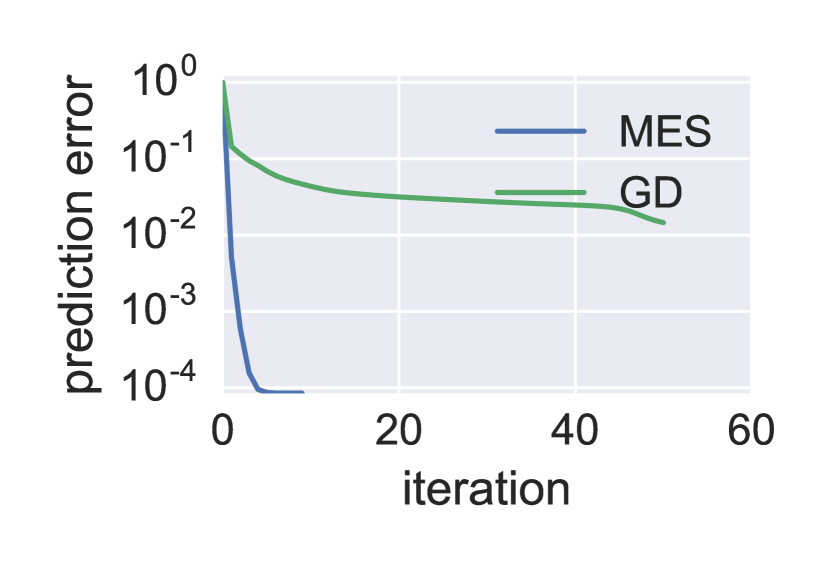
(a) $a=0,\xi=0$

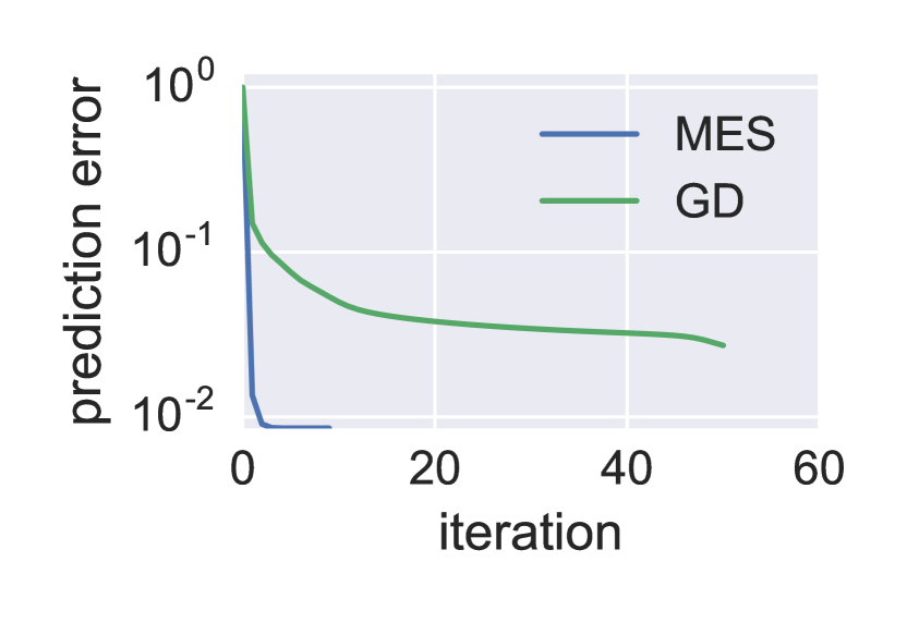
(b) $a=0,\xi=1$

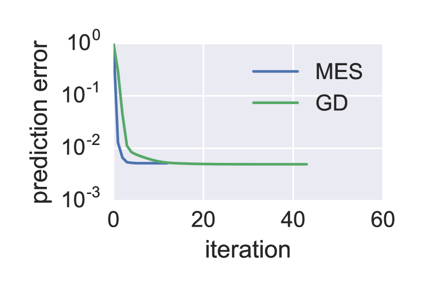
(c) Bernoulli $q=0.01$

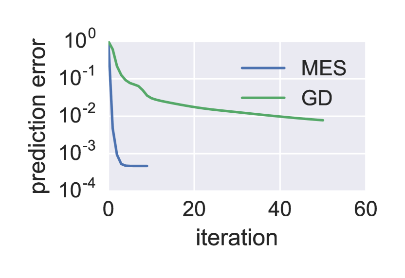
(d) Bernoulli $q=0.1$

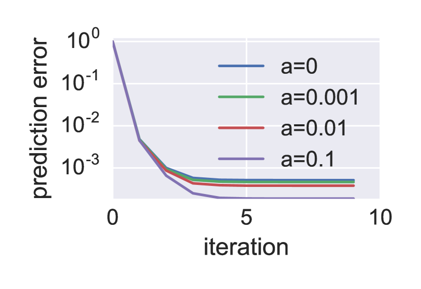
(e) MES on $\xi=0$

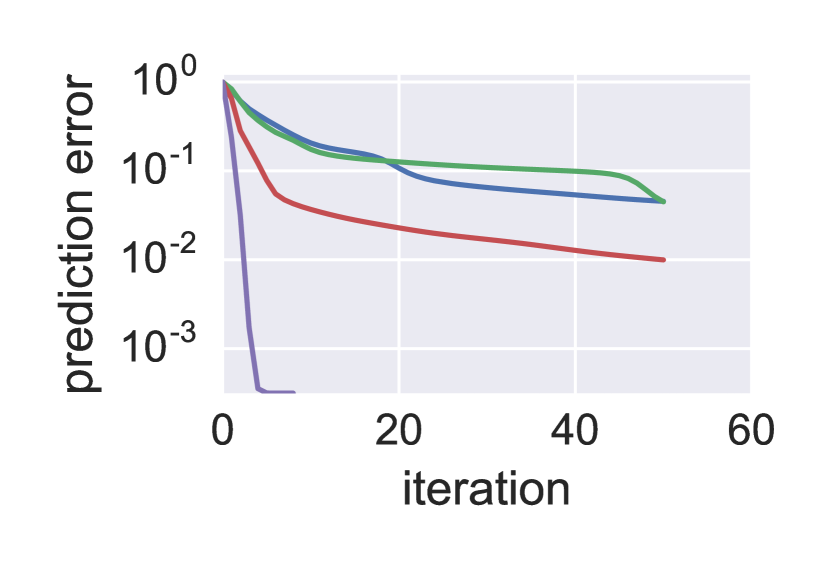
(f) GD on $\xi=0$

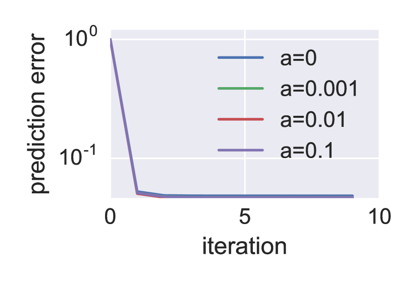
(g) MES on $\xi=1$

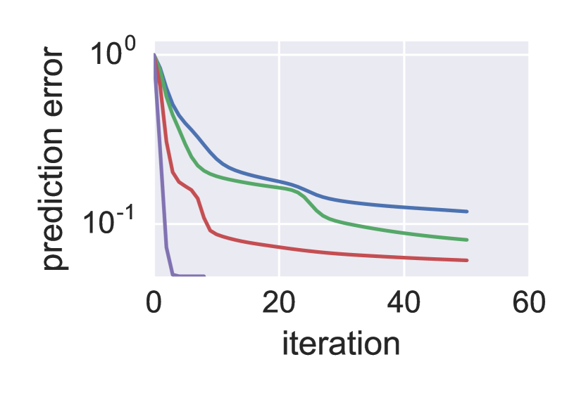
(h) GD on $\xi=1$

Figure 1: Convergence curve. (a)-(b): truncated Gaussian distribution; (c)-(d): Bernoulli distribution; (e)-(h): different truncation level $a$.

In this section, we verify the global convergence rate of Algorithm 1 on MIP and non-MIP distributions. We will show that the naive gradient descent heuristic cannot work well when the distribution is skewed. We implement Algorithm 1 in Python. Our computer has 32 GB memory and a 64 bit, 8 core CPU. Our implementation will be released on our website after publication. In the following figures, we abbreviate Algorithm 1 as MES and the naive gradient descent as GD.

In the following experiments, we choose the dimension $d=1000$ and the rank $k=10$. Since non-MIP distributions require $M^{*}$ to be diagonal-free, we generate $M^{*}$ under two different low-rank models. For MIP distributions, we randomly generate $U\in\mathbb{R}^{d\times k}$ such that $U{}^{\top}U=I$ . Then we produce $M^{*}=UU{}^{\top}$. Please note that our model allows symmetric but non-PSD $M^{*}$ but due to space limitations we only demonstrate the PSD case in this work. For non-MIP distributions, we generate $\bar{M}^{*}=UU{}^{\top}$ similarly and take $M^{*}=\bar{M}^{*}-\mathcal{D}(\bar{M}^{*})$. The $\boldsymbol{w}^{*}$ is randomly sampled from $\mathcal{N}(\boldsymbol{0},1/d)$. The noise term $\boldsymbol{\xi}$ is sampled from $\xi\cdot\mathcal{N}(\boldsymbol{0},I)$ where $\xi$ is the noise level in set $\{0,1\}$. All synthetic experiments are repeated 10 trials in order to report the average performance. In each trial, we randomly sample $30kd$ training instances and $10,000$ testing instances. The running time is measured by the number of iterations. It takes around $7.6$ seconds per iteration on our computer. The estimation accuracy is measured by the normalized mean squared error $[\mathbb{E}(y_{\mathrm{pred}}-y_{\mathrm{true}})^{2}]/\mathbb{E}(y_{\mathrm{true}}^{2})$. We terminate the experiment after $50$ iterations or when the training error decreases less than $10^{-8}$ between two consecutive iterations.

In Figure 1 (a)-(b), we report the convergence curve on truncated Gaussian distribution. To sample $\boldsymbol{x}$, we first generate a Gaussian random number $\hat{x}$ then truncate $x=\min\{\hat{x},a\}$ where $a$ is the truncation level. In Figure 1 (a)-(b) the truncate level $a=0$. Our method MES converges linearly and is significantly faster than GD.

In Figure 1 (c)-(d), we report the convergence curve on Bernoulli distribution which is non-MIP. We set $\mathcal{D}(M^{*})=0$. We choose the binary Bernoulli distribution where $\mathbb{P}(x=1)=q$ otherwise $x=0$. In (c) $q=0.01$ and in (d) $q=0.1$. Again MES converges much faster in both (c) and (d).

As we analyzed in Section 4, the failure of the gradient descent heuristic in the SLM is because the gradient is bias by $O(\|\boldsymbol{\kappa}\|_{\infty})$. We expect the convergence of GD being worse when the skewness of the distribution is larger. To verify this, we report the convergence curves of MES and GD on truncated Gaussian with $a=\{0,10^{-3},0.01,0.1\}$ in Figure 1 (e) and (h) under different noise level. As we expected, when $a\rightarrow 0$ , the skewness becomes larger and GD converges worse. When $a=0$ , GD is unable to find the global optimal solution at all. In contrast, MES always converges globally and linearly under any $a$.

6 Conclusion

We develop the first provable nonconvex algorithm for learning the second order linear model with $O(k^{2}d)$ sampling complexity. This theoretical break-through is built on several recent advances in random matrix theory such as sub-gaussian Hanson-Wright inequality and our novel powerful moment-estimation-sequence method. Our analysis reveals that in high order statistical model, the gradient descent may be sub-optimal due to the gradient bias induced by the high order moments. The proposed MES method is the first efficient tool to eliminate such bias in order to construct a fast convergent sequence for learning high order linear models. We hope this work could inspire future researches of nonconvex high order machines.

Appendix A Preliminary

The $\psi_{2}$-Orlicz norm of a random sub-gaussian variable $z$ is defined by

$$\|z\|_{\psi_{2}}\triangleq\inf\{t>0:\mathbb{E}\exp(z^{2}/t^{2})\leq c\}$$

where $c>0$ is a constant. For a random sub-gaussian vector $\boldsymbol{z}\in\mathbb{R}^{n}$, its $\psi_{2}$-Orlicz norm is

$$\|\boldsymbol{z}\|_{\psi_{2}}\triangleq\sup_{\boldsymbol{x}\in S^{n-1}}\|\left\langle\boldsymbol{z},\boldsymbol{x}\right\rangle\|_{\psi_{2}}$$

where $S^{n-1}$ is the unit sphere.

The following theorem gives the matrix Bernstein’s inequality Roman Vershynin [2017].

Theorem 9 (Matrix Bernstein’s inequality).

Let $X_{1},\cdots,X_{N}$ be independent, mean zero $d\times n$ random matrices with $d\geq n$ and $\|X_{i}\|_{2}\leq B$. Denote

$$\sigma^{2}\triangleq\max\{\|\sum_{i=1}^{N}\mathbb{E}X_{i}X_{i}{}^{\top}\|_{2},\|\sum_{i=1}^{N}\mathbb{E}X_{i}{}^{\top}X_{i}\|_{2}\}\ .$$

Then for any $t\geq 0$, we have

$$\mathbb{P}(\|\sum_{i=1}^{N}X_{i}\|_{2}\geq t)\leq 2d\exp\left[-c\min\left(\frac{t^{2}}{\sigma^{2}},\frac{t}{B}\right)\right]\ .$$

where $c$ is a universal constant. Equivalently, with probability at least $1-\eta$,

$$\|\sum_{i=1}^{N}X_{i}\|_{2}\leq c\max\left\{B\log(2d/\eta),\sigma\sqrt{\log(2d/\eta)}\right\}\ .$$

When $\mathbb{E}X_{i}\not=\boldsymbol{0}$, replacing $X_{i}$ with $X_{i}-\mathbb{E}X_{i}$ the inequality still holds true.

The following Hanson-Wright inequality for sub-gaussian variables is given in Rudelson and Vershynin [2013] .

Theorem 10 (Sub-gaussian Hanson-Wright inequality).

Let $\boldsymbol{x}=[x_{1},\cdots,x_{d}]\in\mathbb{R}^{d}$ be a random vector with independent, mean zero, sub-gaussian coordinates. Then given a fixed $d\times d$ matrix $M$, for any $t\geq 0$,

$$\mathbb{P}\left\{|\boldsymbol{x}{}^{\top}A\boldsymbol{x}-\mathbb{E}\boldsymbol{x}{}^{\top}A\boldsymbol{x}|\geq t\right\}\leq 2\exp\left[-c\min\left(\frac{t^{2}}{B^{4}\|A\|_{F}^{2}},\frac{t}{B^{2}\|A\|_{2}}\right)\right]\ ,$$

where $B=\max_{i}\|X_{i}\|_{\psi_{2}}$ and $c$ is a universal positive constant. Equivalently, with probability at least $1-\eta$,

$$|\boldsymbol{x}{}^{\top}A\boldsymbol{x}-\mathbb{E}\boldsymbol{x}{}^{\top}A\boldsymbol{x}|\leq c\max\{B^{2}\|A\|_{2}\log(2/\eta),B^{2}\|A\|_{F}\sqrt{\log(2/\eta)}\}\ .$$

The next lemma estimates the covering number of low-rank matrices Candes and Plan [2011].

Lemma 11 (Covering number of low-rank matrices).

Let $S=\{M\in\mathbb{R}^{d\times d}:\mathrm{rank}(M)\leq k,\|M\|_{F}\leq c\}$ be the set of rank-$k$ matrices with unit Frobenius norm. Then there is an $\epsilon$-net cover of $S$, denoted as $\bar{S}(\epsilon)$, such that

$$|\bar{S}(\epsilon)|\leq(9c/\epsilon)^{(2d+1)k}\ .$$

Note that the original lemma in Candes and Plan [2011] bounds $\|M\|_{F}=1$ but in the above lemma we slightly relax to $\|M\|_{F}\leq c$ . The proof is nearly the same as the original one.

Truncation trick

As Bernstein’s inequality requires boundness of the random variable, we use the truncation trick in order to apply it on unbounded random matrices. First we condition on the tail distribution of random matrices to bound the norm of a fixed random matrix. Then we take union bound over all $n$ random matrices in the summation. The union bound will result in an extra $O[\log(n)]$ penalty in the sampling complexity which can be absorbed into $C_{\eta}$ or $c_{\eta}$ . Please check [Tao, 2012] for more details.

Appendix B Proof of Theorem 5

Define $p_{1}=2+\|\boldsymbol{\phi}^{*}-3\|_{\infty}$ . Recall that

$$\frac{1}{n}\mathcal{A}^{\prime}\mathcal{A}(M)= \frac{1}{n}\sum_{i=1}^{n}\boldsymbol{x}^{(i)}\boldsymbol{x}^{(i)}{}^{\top}M\boldsymbol{x}^{(i)}\boldsymbol{x}^{(i)}{}^{\top}\ .$$

Denote

$$Z_{i}\triangleq\boldsymbol{x}^{(i)}\boldsymbol{x}^{(i)}{}^{\top}M\boldsymbol{x}^{(i)}\boldsymbol{x}^{(i)}{}^{\top}$$

$$\mathbb{E}Z_{i}=2M+\mathrm{tr}(M)I+\mathcal{D}(\boldsymbol{\phi}^{*}-3)\mathcal{D}(M)\ .$$

In order to apply matrix Bernstein’s inequality , we have

$$\|Z_{i}\|_{2}= \|\boldsymbol{x}^{(i)}\boldsymbol{x}^{(i)}{}^{\top}M\boldsymbol{x}^{(i)}\boldsymbol{x}^{(i)}{}^{\top}\|_{2}$$

$$\leq |\boldsymbol{x}^{(i)}{}^{\top}M\boldsymbol{x}^{(i)}|\|\boldsymbol{x}^{(i)}\boldsymbol{x}^{(i)}{}^{\top}\|_{2}$$

$$\leq |\boldsymbol{x}^{(i)}{}^{\top}M\boldsymbol{x}^{(i)}|\|\boldsymbol{x}^{(i)}\|_{2}^{2}$$

$$\leq c_{\eta}[\|M\|_{F}+|\mathrm{tr}(M)|]\|\boldsymbol{x}^{(i)}\|_{2}^{2}$$

$$\leq c_{\eta}[\|M\|_{F}+|\mathrm{tr}(M)|]d\ .$$

And

$$\|\mathbb{E}Z_{i}\|_{2}= \|2M+\mathrm{tr}(M)I+\mathcal{D}(\boldsymbol{\phi}^{*}-3)\mathcal{D}(M)\|_{2}$$

$$\leq 2\|M\|_{2}+|\mathrm{tr}(M)|+\|\boldsymbol{\phi}^{*}-3\|_{\infty}\|M\|_{2}$$

$$\leq (2+\|\boldsymbol{\phi}^{*}-3\|_{\infty})\|M\|_{2}+|\mathrm{tr}(M)|$$

$$\leq p_{1}\|M\|_{2}+|\mathrm{tr}(M)|\ .$$

And

$$\|\mathbb{E}Z_{i}Z_{i}{}^{\top}\|_{2}= \|\mathbb{E}\boldsymbol{x}^{(i)}\boldsymbol{x}^{(i)}{}^{\top}M\boldsymbol{x}^{(i)}\boldsymbol{x}^{(i)}{}^{\top}\boldsymbol{x}^{(i)}\boldsymbol{x}^{(i)}{}^{\top}M\boldsymbol{x}^{(i)}\boldsymbol{x}^{(i)}{}^{\top}\|_{2}$$

$$\leq c_{\eta}d\|\mathbb{E}\boldsymbol{x}^{(i)}\boldsymbol{x}^{(i)}{}^{\top}M\boldsymbol{x}^{(i)}\boldsymbol{x}^{(i)}{}^{\top}M\boldsymbol{x}^{(i)}\boldsymbol{x}^{(i)}{}^{\top}\|_{2}$$

$$\leq c_{\eta}d\|\mathbb{E}\boldsymbol{x}^{(i)}\boldsymbol{x}^{(i)}{}^{\top}\|_{2}|\boldsymbol{x}^{(i)}{}^{\top}M\boldsymbol{x}^{(i)}|^{2}$$

$$\leq c_{\eta}d\|\mathbb{E}\boldsymbol{x}^{(i)}\boldsymbol{x}^{(i)}{}^{\top}\|_{2}[\|M\|_{F}+|\mathrm{tr}(M)|]^{2}$$

$$\leq c_{\eta}d[\|M\|_{F}+|\mathrm{tr}(M)|]^{2}\ .$$

And

$$\|(\mathbb{E}Z_{i})(\mathbb{E}Z_{i}){}^{\top}\|_{2}\leq \|\mathbb{E}Z_{i}\|_{2}^{2}$$

$$\leq [p_{1}\|M\|_{2}+|\mathrm{tr}(M)|]^{2}\ .$$

Therefore we get

$$\|Z_{i}-\mathbb{E}Z_{i}\|_{2}\leq \|Z_{i}\|_{2}+\|\mathbb{E}Z_{i}\|_{2}$$

$$\leq c_{\eta}[\|M\|_{F}+|\mathrm{tr}(M)|]d+p_{1}\|M\|_{2}+|\mathrm{tr}(M)|\ .$$

And

$$\mathrm{Var}1\triangleq \|(Z_{i}-\mathbb{E}Z_{i})(Z_{i}-\mathbb{E}Z_{i}){}^{\top}\|_{2}$$

$$\leq \|Z_{i}Z_{i}{}^{\top}\|_{2}+\|(\mathbb{E}Z_{i})(\mathbb{E}Z_{i}){}^{\top}\|_{2}$$

$$\leq c_{\eta}d[\|M\|_{F}+|\mathrm{tr}(M)|]^{2}+[p_{1}\|M\|_{2}+|\mathrm{tr}(M)|]^{2}\ .$$

Suppose that

$$d[\|M\|_{F}+|\mathrm{tr}(M)|]^{2}\geq[p_{1}\|M\|_{2}+|\mathrm{tr}(M)|]^{2}$$

$$\Leftarrow d[\|M\|_{2}+|\mathrm{tr}(M)|]^{2}\geq[p_{1}\|M\|_{2}+|\mathrm{tr}(M)|]^{2}$$

$$\Leftarrow d[\|M\|_{2}+|\mathrm{tr}(M)|]^{2}\geq p_{1}^{2}[\|M\|_{2}+|\mathrm{tr}(M)|]^{2}$$

$$\Leftarrow d\geq p_{1}^{2}\ .$$

And suppose that

$$[\|M\|_{F}+|\mathrm{tr}(M)|]d\geq p_{1}\|M\|_{2}+|\mathrm{tr}(M)|$$

$$\Leftarrow d\geq p_{1}$$

$$\Leftarrow d\geq p_{1}^{2}\ .$$

The we get

$$\|Z_{i}-\mathbb{E}Z_{i}\|_{2}\leq c_{\eta}[\|M\|_{F}+|\mathrm{tr}(M)|]d$$

$$\leq c_{\eta}kd\|M\|_{2}$$

$$\mathrm{Var}1\leq c_{\eta}d[\|M\|_{F}+|\mathrm{tr}(M)|]^{2}$$

$$\leq c_{\eta}k^{2}d\|M\|_{2}^{2}\ .$$

Then according to matrix Bernstein’s inequality,

$$\|\frac{1}{n}\sum_{i=1}^{n}Z_{i}-\mathbb{E}Z_{i}\|_{2}= c_{\eta}\max\{\frac{1}{n}kd\|M\|_{2},\frac{1}{\sqrt{n}}\sqrt{k^{2}d}\|M\|_{2}\}$$

$$\leq c_{\eta}\frac{1}{\sqrt{n}}\sqrt{k^{2}d}\|M\|_{2}\ .$$

provided

$$\frac{1}{n}kd\|M\|_{2}\leq\frac{1}{\sqrt{n}}\sqrt{k^{2}d}\|M\|_{2}$$

$$\Leftarrow n\geq d\ .$$

Choose $n\geq c_{\eta}k^{2}d/\delta^{2}$, we getv

$$\|\frac{1}{n}\sum_{i=1}^{n}Z_{i}-\mathbb{E}Z_{i}\|_{2}\leq \delta\|M\|_{2}\ .$$

Appendix C Proof of Lemma 6

Proof.

To prove $\frac{1}{n}\mathcal{A}^{\prime}(X{}^{\top}\boldsymbol{w})$,

$$\frac{1}{n}\mathcal{A}^{\prime}(X{}^{\top}\boldsymbol{w})= \frac{1}{n}\sum_{i=1}^{n}\boldsymbol{x}^{(i)}\boldsymbol{x}^{(i)}{}^{\top}\boldsymbol{w}\boldsymbol{x}^{(i)}{}^{\top}\ .$$

Similar to Theorem 5, just replacing $\mathcal{A}(M)$ with $\boldsymbol{w}$, then with probability at last $1-\eta$,

$$\|\frac{1}{n}\mathcal{A}^{\prime}(X{}^{\top}\boldsymbol{w})-\mathcal{D}(\boldsymbol{\kappa}^{*})\boldsymbol{w}\|_{2}\leq C_{\eta}\sqrt{d/n}\|\boldsymbol{w}\|_{2}\ .$$

Therefore let

$$n\geq C_{\eta}d/\delta^{2}\ .$$

We have

$$\|\frac{1}{n}\mathcal{A}^{\prime}(X{}^{\top}\boldsymbol{w})-\mathcal{D}(\boldsymbol{\kappa}^{*})\boldsymbol{w}\|_{2}\leq\delta\|\boldsymbol{w}\|_{2}\ .$$

To prove $\mathcal{P}^{(0)}(\boldsymbol{y})$,

$$\mathcal{P}^{(0)}(\boldsymbol{y})= \frac{1}{n}\sum_{i=1}^{n}\boldsymbol{x}^{(i)}{}^{\top}\boldsymbol{w}+\frac{1}{n}\sum_{i=1}^{n}\boldsymbol{x}^{(i)}{}^{\top}M\boldsymbol{x}^{(i)}\ .$$

Since $\boldsymbol{x}$ is coordinate sub-gaussian, any $i\in\{1,\cdots,d\}$, with probability at least $1-\eta$,

$$\|\boldsymbol{x}^{(i)}{}^{\top}\boldsymbol{w}\|_{2}\leq c\sqrt{d}\|\boldsymbol{w}\|_{2}\log(n/\eta)\ .$$

Then we have

$$\|\frac{1}{n}\sum_{i=1}^{n}\boldsymbol{x}^{(i)}{}^{\top}\boldsymbol{w}-0\|_{2}\leq C\sqrt{d}\|\boldsymbol{w}\|_{2}\log(n/\eta)/\sqrt{n}\ .$$

Choose $n\geq c_{\eta}d$, we get

$$\|\frac{1}{n}\sum_{i=1}^{n}\boldsymbol{x}^{(i)}{}^{\top}\boldsymbol{w}\|_{2}\leq \delta\|\boldsymbol{w}\|_{2}\ .$$

From Hanson-Wright inequality,

$$\|\frac{1}{n}\sum_{i=1}^{n}\boldsymbol{x}^{(i)}{}^{\top}M\boldsymbol{x}^{(i)}-\mathrm{tr}(M)\|_{2}\leq C\|M\|_{F}\log(1/\eta)$$

$$\leq C\|M\|_{2}\sqrt{k/n}\log(1/\eta)\ .$$

Therefore

$$\mathcal{P}^{(0)}(\boldsymbol{y})= \mathrm{tr}(M)+O[(\sqrt{d}\|\boldsymbol{w}\|_{2}+\|M\|_{2}\sqrt{k})/\sqrt{n}\log(n/\eta)]$$

$$= \mathrm{tr}(M)+O[C_{\eta}(\sqrt{d}\|\boldsymbol{w}\|_{2}+\|M\|_{2}\sqrt{k})/\sqrt{n}]$$

$$= \mathrm{tr}(M)+O[C_{\eta}(\|\boldsymbol{w}\|_{2}+\|M\|_{2}\sqrt{k})\sqrt{d/n}]\ .$$

Let

$$n\geq C_{\eta}kd/\delta^{2}\ .$$

We have

$$\mathcal{P}^{(0)}(\boldsymbol{y})= \mathrm{tr}(M)+O[\delta(\|\boldsymbol{w}\|_{2}+\|M\|_{2})]\ .$$

To prove $\mathcal{P}^{(1)}(\boldsymbol{y})$,

$$\mathcal{P}^{(1)}(\boldsymbol{y})= \frac{1}{n}\sum_{i=1}^{n}\boldsymbol{x}^{(i)}\boldsymbol{x}^{(i)}{}^{\top}\boldsymbol{w}+\frac{1}{n}\sum_{i=1}^{n}\boldsymbol{x}^{(i)}\boldsymbol{x}^{(i)}{}^{\top}M\boldsymbol{x}^{(i)}\ .$$

From covariance concentration inequality,

$$\|\frac{1}{n}\sum_{i=1}^{n}\boldsymbol{x}^{(i)}\boldsymbol{x}^{(i)}{}^{\top}\boldsymbol{w}-\boldsymbol{w}\|_{2}\leq c\sqrt{d/n}\|\boldsymbol{w}\|_{2}\log(d/\eta)$$

$$\leq C_{\eta}\sqrt{d/n}\|\boldsymbol{w}\|_{2}\ .$$

To bound the second term in $\mathcal{P}^{(1)}(\boldsymbol{y})$, apply Hanson-Wright inequality again,

$$\|\boldsymbol{x}^{(i)}\boldsymbol{x}^{(i)}{}^{\top}M\boldsymbol{x}^{(i)}\|_{2}\leq \|\boldsymbol{x}^{(i)}\|_{2}\|\boldsymbol{x}^{(i)}{}^{\top}M\boldsymbol{x}^{(i)}\|_{2}$$

$$\leq c[\|M\|_{F}+\mathrm{tr}(M)]\sqrt{d}\log^{2}(nd/\eta)$$

$$\leq C_{\eta}k\|M\|_{2}\sqrt{d}\ .$$

By matrix Chernoff’s inequality, choose $n\geq c_{\eta}k^{2}d/\delta^{2}$,

$$\|\frac{1}{n}\sum_{i=1}^{n}\boldsymbol{x}^{(i)}\boldsymbol{x}^{(i)}{}^{\top}M\boldsymbol{x}^{(i)}-\mathcal{D}(M)\boldsymbol{\kappa}^{*}\|_{2}\leq C_{\eta}k\|M\|_{2}\sqrt{d/n}$$

$$\leq \delta\|M\|_{2}\ .$$

Therefore we have

$$\mathcal{P}^{(1)}(\boldsymbol{y})=\boldsymbol{w}+\mathcal{D}(M)\boldsymbol{\kappa}^{*}+O [\delta(\|\boldsymbol{w}\|_{2}+\|M\|_{2})]\ .$$

To bound $\mathcal{P}^{(2)}(\boldsymbol{y})$ , first note that

$$\mathcal{P}^{(2)}(\boldsymbol{y})= \frac{1}{n}\sum_{i=1}^{n}\boldsymbol{x}^{(i)2}\boldsymbol{x}^{(i)}{}^{\top}\boldsymbol{w}+\frac{1}{n}\sum_{i=1}^{n}\boldsymbol{x}^{(i)2}\boldsymbol{x}^{(i)}{}^{\top}M\boldsymbol{x}^{(i)}-P^{(0)}(\boldsymbol{y})$$

$$= \frac{1}{n}\sum_{i=1}^{n}\mathcal{D}(\boldsymbol{x}^{(i)}\boldsymbol{x}^{(i)}{}^{\top}\boldsymbol{w}\boldsymbol{x}^{(i)})+\frac{1}{n}\sum_{i=1}^{n}\mathcal{D}(\boldsymbol{x}^{(i)}\boldsymbol{x}^{(i)}{}^{\top}M\boldsymbol{x}^{(i)}\boldsymbol{x}^{(i)}{}^{\top})-P^{(0)}(\boldsymbol{y})\ .$$

Then similarly,

$$\|\frac{1}{n}\sum_{i=1}^{n}\boldsymbol{x}^{(i)2}\boldsymbol{x}^{(i)}{}^{\top}\boldsymbol{w}-\mathcal{D}(\boldsymbol{\kappa}^{*})\boldsymbol{w}\|_{2}\leq C_{\eta}\sqrt{d/n}\|\boldsymbol{w}\|_{2}$$

$$\|\frac{1}{n}\sum_{i=1}^{n}\boldsymbol{x}^{(i)2}\boldsymbol{x}^{(i)}{}^{\top}M\boldsymbol{x}^{(i)}-\mathrm{tr}(M)-\mathcal{D}(M)(\boldsymbol{\phi}^{*}-1)\|_{2}\leq C_{\eta}k\|M\|_{2}\sqrt{d/n}\ .$$

The last inequality is because Theorem 5. Combine all together, choose $n\geq c_{\eta}k^{2}d$,

$$\mathcal{P}^{(2)}(\boldsymbol{y})= \mathcal{D}(\boldsymbol{\kappa}^{*})\boldsymbol{w}+\mathcal{D}(M)(\boldsymbol{\phi}^{*}-1)+O(C_{\eta}\sqrt{d/n}\|\boldsymbol{w}\|_{2})$$

$$+O(\|M\|_{2}k\sqrt{d/n})+O[C_{\eta}(\|\boldsymbol{w}\|_{2}+k\|M\|_{2})\sqrt{d/n}]$$

$$= \mathcal{D}(\boldsymbol{\kappa}^{*})\boldsymbol{w}+\mathcal{D}(M)(\boldsymbol{\phi}^{*}-1)+O[C_{\eta}(\|\boldsymbol{w}\|_{2}+\|M\|_{2})k\sqrt{d/n}]$$

$$= \mathcal{D}(\boldsymbol{\kappa}^{*})\boldsymbol{w}+\mathcal{D}(M)(\boldsymbol{\phi}^{*}-1)+O[\delta(\|\boldsymbol{w}\|_{2}+\|M\|_{2})]\ .$$

∎

Appendix D Proof of Lemma 7

The next lemma bounds the estimation accuracy of $\boldsymbol{\kappa}^{*},\boldsymbol{\phi}^{*}$ . It directly follows sub-gaussian concentration inequality and union bound.

Lemma 12.

Given $n$ i.i.d. sampled $\boldsymbol{x}^{(i)}$, $i\in\{1,\cdots,n\}$. With a probability at least $1-\eta$,

$$\|\boldsymbol{\kappa}-\boldsymbol{\kappa}^{*}\|_{\infty}\leq C_{\eta}/\sqrt{n}$$

$$\|\boldsymbol{\phi}-\boldsymbol{\phi}^{*}\|_{\infty}\leq C_{\eta}/\sqrt{n}$$

provided $n\geq C_{\eta}d$ .

Denote $G^{*}$ as $G$ in Eq. (6) but computed with $\boldsymbol{\kappa}^{*},\boldsymbol{\phi}^{*}$. The next lemma bounds $\|G_{j,:}-G_{j,:}^{*}\|_{2}$ for any $j\in\{1,\cdots,d\}$.

Proof.

Denote $\boldsymbol{g}=G_{j}$, $\boldsymbol{g}^{*}=G_{j}^{*}$, $\kappa=\boldsymbol{\kappa}_{j}$, $\mathbf{\phi=\boldsymbol{\phi}}_{j}$,

$$A= \left[\begin{array}[]{cc}1&\boldsymbol{\kappa}_{j}\\ \boldsymbol{\kappa}_{j}&\boldsymbol{\phi}_{j}-1\end{array}\right],\ \boldsymbol{b}=\left[\begin{array}[]{c}\boldsymbol{\kappa}_{j}\\ \boldsymbol{\phi}_{j}-3\end{array}\right]$$

$$A^{*}= \left[\begin{array}[]{cc}1&\boldsymbol{\kappa}_{j}^{*}\\ \boldsymbol{\kappa}_{j}^{*}&\boldsymbol{\phi}_{j}^{*}-1\end{array}\right],\ \boldsymbol{b}^{*}=\left[\begin{array}[]{c}\boldsymbol{\kappa}_{j}^{*}\\ \boldsymbol{\phi}_{j}^{*}-3\end{array}\right]\ .$$

Then $\boldsymbol{g}=A^{-1}\boldsymbol{b}$, $\boldsymbol{g}^{*}=A^{*-1}\boldsymbol{b}^{*}$ . Since $\mathbb{P}(\boldsymbol{x})$ is $\tau$-MIP, $\|A^{*-1}\|_{2}\leq 1/\tau$ . From Lemma 12,

$$\|A-A^{*}\|_{2}\leq C\log(d/\eta)/\sqrt{n}$$

$$\|\boldsymbol{b}-\boldsymbol{b}^{*}\|_{2}\leq C\log(d/\eta)/\sqrt{n}\ .$$

Define $\Delta_{A}\triangleq A-A^{*}$, $\Delta_{b}\triangleq\boldsymbol{b}-\boldsymbol{b}^{*}$, $\Delta_{g}\triangleq\boldsymbol{g}-\boldsymbol{g}^{*}$,

$$A\boldsymbol{g}=\boldsymbol{b}$$

$$\Leftrightarrow (A^{*}+\Delta_{A})(\boldsymbol{g}^{*}+\Delta_{g})=\boldsymbol{b}^{*}+\Delta_{b}$$

$$\Leftrightarrow A^{*}\Delta_{g}+\Delta_{A}\boldsymbol{g}^{*}+\Delta_{A}\Delta_{g}=\Delta_{b}$$

$$\Leftrightarrow (A^{*}+\Delta_{A})\Delta_{g}=\Delta_{b}-\Delta_{A}\boldsymbol{g}^{*}$$

$$\Rightarrow \|(A^{*}+\Delta_{A})\Delta_{g}\|_{2}=\|\Delta_{b}-\Delta_{A}\boldsymbol{g}^{*}\|_{2}$$

$$\Rightarrow \|(A^{*}+\Delta_{A})\Delta_{g}\|_{2}\leq\|\Delta_{b}\|_{2}+\|\Delta_{A}\boldsymbol{g}^{*}\|_{2}$$

$$\Rightarrow \|(A^{*}+\Delta_{A})\Delta_{g}\|_{2}\leq C\log(d/\eta)/\sqrt{n}+C\log(d/\eta)/\sqrt{n}\|\boldsymbol{g}^{*}\|_{2}$$

$$\Rightarrow \|(A^{*}+\Delta_{A})\Delta_{g}\|_{2}\leq C\log(d/\eta)/\sqrt{n}(1+\|\boldsymbol{g}^{*}\|_{2})$$

$$\Rightarrow \|(A^{*}+\Delta_{A})\Delta_{g}\|_{2}\leq C\log(d/\eta)/\sqrt{n}(1+\frac{1}{\tau}\|\boldsymbol{b}^{*}\|_{2})$$

$$\Rightarrow \|(A^{*}+\Delta_{A})\Delta_{g}\|_{2}\leq C\log(d/\eta)/\sqrt{n}(1+\frac{1}{\tau}\sqrt{\kappa^{2}+(\phi-3)^{2}})$$

$$\Rightarrow [\tau-C\log(d)/\sqrt{n}]\|\Delta_{g}\|_{2}\leq C\log(d/\eta)/\sqrt{n}(1+\frac{1}{\tau}\sqrt{\kappa^{2}+(\phi-3)^{2}})\ .$$

When

$$\tau-C\log(d/\eta)/\sqrt{n}\geq\frac{1}{2}\tau$$

$$\Leftrightarrow n\geq 4C^{2}\log^{2}(d/\eta)/\tau^{2}\ ,$$

we have

$$\|\Delta_{g}\|_{2}\leq \frac{2C}{\tau\sqrt{n}}\log(d/\eta)(1+\frac{1}{\tau}\sqrt{\kappa^{2}+(\phi-3)^{2}})\ .$$

Since $\Delta_{g}$ is a vector of dimension 2, its $\ell_{2}$-norm bound also controls its $\ell_{\infty}$-norm bound up to constant. Choose

$$n\geq C_{\eta}\frac{1}{\tau}(1+\frac{1}{\tau}\sqrt{\kappa^{2}+(\phi-3)^{2}})/\delta^{2}\ .$$

We have

$$\|\Delta_{g}\|_{\infty}\leq \delta\ .$$

The proof of $H$ is similar. ∎

Appendix E Proof of Lemma 8

Proof.

To abbreviate the notation, we omit $\hat{\boldsymbol{y}}^{(t)}-\boldsymbol{y}^{(t)}$ and superscript $t$ in the following proof. Denote $\mathcal{H}^{*}=\mathbb{E}\mathcal{H}$ and the expectation of other operators similarly. By construction in Algorithm 2,

$$\mathcal{M}\triangleq \mathcal{H}-\frac{1}{2}\mathcal{D}(G_{1}\circ\mathcal{P}^{(1)})-\frac{1}{2}\mathcal{D}(G_{2}\circ\mathcal{P}^{(2)})$$

$$= \mathcal{H}^{*}+O[\delta(\alpha_{t-1}+\beta_{t-1})]$$

$$-\frac{1}{2}\mathcal{D}(G_{1}^{*}\circ\mathcal{P}^{*(1)})-\frac{1}{2}\mathcal{D}(G_{2}^{*}\circ\mathcal{P}^{*(2)})$$

$$+O[\|G-G^{*}\|_{\infty}(\|\mathcal{P}^{*(1)}\|_{2}+\|\mathcal{P}^{*(2)}\|_{2})]$$

$$+O[\|G-G^{*}\|_{\infty}\delta(\alpha_{t-1}+\beta_{t-1})]$$

$$= M^{(t)}-M^{*}+O[\delta(\alpha_{t-1}+\beta_{t-1})]$$

$$+O[\delta(\|\mathcal{P}^{*(1)}\|_{2}+\|\mathcal{P}^{*(2)}\|_{2})]$$

$$+O[\delta^{2}(\alpha_{t-1}+\beta_{t-1})]$$

$$= M^{(t)}-M^{*}+O[\delta(\alpha_{t-1}+\beta_{t-1})]$$

$$+O[\delta(\|\mathcal{P}^{*(1)}\|_{2}+\|\mathcal{P}^{*(2)}\|_{2})]$$

$$= M^{(t)}-M^{*}+O[\delta(\alpha_{t-1}+\beta_{t-1})]$$

$$+O[\delta(\alpha_{t-1}\|\boldsymbol{\kappa}^{*}\|_{\infty}+\beta_{t-1})$$

$$+\alpha_{t-1}\|\boldsymbol{\phi}^{*}-1\|_{\infty}+\beta_{t-1}\|\boldsymbol{\kappa}^{*}\|_{\infty}]$$

$$= M^{(t)}-M^{*}+O[\delta(\alpha_{t-1}+\beta_{t-1})]+O[\delta p(\alpha_{t-1}+\beta_{t-1})]$$

$$= M^{(t)}-M^{*}+O[\delta(p+1)(\alpha_{t-1}+\beta_{t-1})]\ .$$

The above requires

$$n\geq \max\{C_{\eta}\frac{1}{\tau}(1+\frac{1}{\tau}\sqrt{\kappa^{2}+(\phi-3)^{2}})/\delta^{2},C_{\eta}k^{2}d\}$$

$$= \max\{C_{\eta}p(\tau\delta)^{-2},C_{\eta}k^{2}d\}\ .$$

Replace $\delta(p+1)$ with $\delta$, the proof is completed.

To bound $\mathcal{W}^{(t)}(\hat{\boldsymbol{y}}^{(t)}-\boldsymbol{y}^{(t)})$, similarly we have

$$\mathcal{W}= G_{1}\circ\mathcal{P}^{(1)}+G_{2}\circ\mathcal{P}^{(2)}$$

$$= G_{1}^{*}\circ\mathcal{P}^{*(1)}+G_{2}^{*}\circ\mathcal{P}^{*(2)}$$

$$+O[\|G-G^{*}\|_{\infty}\delta(\alpha_{t-1}+\beta_{t-1})]$$

$$+O[\|G-G^{*}\|_{\infty}(\|\mathcal{P}^{*(1)}\|_{2}+\|\mathcal{P}^{*(2)}\|_{2})]$$

$$= \boldsymbol{w}^{(t-1)}-\boldsymbol{w}^{*}+O[\delta^{2}(\alpha_{t-1}+\beta_{t-1})]$$

$$+O[\delta p(\alpha_{t-1}+\beta_{t-1})]$$

$$= \boldsymbol{w}^{(t-1)}-\boldsymbol{w}^{*}+O[\delta(p+1)(\alpha_{t-1}+\beta_{t-1})]\ .$$

∎

References

- Bayer [2016] Immanuel Bayer. fastFM: A Library for Factorization Machines. Journal of Machine Learning Research, 17(184):1–5, 2016.
- Blondel et al. [2016] Mathieu Blondel, Masakazu Ishihata, Akinori Fujino, and Naonori Ueda. Polynomial Networks and Factorization Machines: New Insights and Efficient Training Algorithms. In Proceedings of The 33rd International Conference on Machine Learning, pages 850–858, 2016.
- Cai and Zhang [2015] T. Tony Cai and Anru Zhang. ROP: Matrix recovery via rank-one projections. The Annals of Statistics, 43(1):102–138, 2015.
- Candes et al. [2013] E. Candes, Y. Eldar, T. Strohmer, and V. Voroninski. Phase Retrieval via Matrix Completion. SIAM Journal on Imaging Sciences, 6(1):199–225, 2013.
- Candes and Plan [2011] E. J. Candes and Y. Plan. Tight Oracle Inequalities for Low-Rank Matrix Recovery From a Minimal Number of Noisy Random Measurements. IEEE Transactions on Information Theory, 57(4):2342–2359, 2011.
- Hofmann et al. [2008] Thomas Hofmann, Bernhard Schölkopf, and Alexander J. Smola. Kernel methods in machine learning. The Annals of Statistics, 36(3):1171–1220, 2008.
- Jain and Dhillon [2013] Prateek Jain and Inderjit S. Dhillon. Provable inductive matrix completion. arXiv preprint arXiv:1306.0626, 2013.
- Koltchinskii [2011] V. Koltchinskii. Oracle Inequalities in Empirical Risk Minimization and Sparse Recovery Problems, volume 2033. Springer, 2011.
- Kueng et al. [2017] Richard Kueng, Holger Rauhut, and Ulrich Terstiege. Low rank matrix recovery from rank one measurements. Applied and Computational Harmonic Analysis, 42(1):88–116, 2017.
- Ming Lin and Jieping Ye [2016] Ming Lin and Jieping Ye. A Non-convex One-Pass Framework for Generalized Factorization Machine and Rank-One Matrix Sensing. In NIPS, 2016.
- Nesterov [2004] Yurii Nesterov. Introductory Lectures on Convex Optimization: A Basic Course, volume 87. Springer, 2004.
- Rendle [2010] Steffen Rendle. Factorization machines. In IEEE 10th International Conference On Data Mining, pages 995–1000, 2010.
- Rendle [2012] Steffen Rendle. Factorization Machines with libFM. ACM Trans. Intell. Syst. Technol., 3(3):57:1–57:22, 2012.
- Roman Vershynin [2017] Roman Vershynin. High-Dimensional Probability: An Introduction with Applications in Data Science. 2017.
- Rudelson and Vershynin [2013] Mark Rudelson and Roman Vershynin. Hanson-Wright inequality and sub-gaussian concentration. Electronic Communications in Probability, 18, 2013.
- Tao [2012] Terence Tao. Topics in Random Matrix Theory, volume 132. Amer Mathematical Society, 2012.
- Tropp [2015] Joel A. Tropp. Convex Recovery of a Structured Signal from Independent Random Linear Measurements. In Sampling Theory, a Renaissance, Applied and Numerical Harmonic Analysis, pages 67–101. Springer International Publishing, 2015.
- Vedaldi and Zisserman [2012] A. Vedaldi and A. Zisserman. Efficient Additive Kernels via Explicit Feature Maps. IEEE Transactions on Pattern Analysis and Machine Intelligence, 34(3):480 –492, 2012.
- Zhao et al. [2015] Tuo Zhao, Zhaoran Wang, and Han Liu. A Nonconvex Optimization Framework for Low Rank Matrix Estimation. In NIPS, pages 559–567. 2015.