Compositional Falsification of Cyber-Physical Systems with Machine Learning Components

Abstract

Cyber-physical systems (CPS), such as automotive systems, are starting to include sophisticated machine learning (ML) components. Their correctness, therefore, depends on properties of the inner ML modules. While learning algorithms aim to generalize from examples, they are only as good as the examples provided, and recent efforts have shown that they can produce inconsistent output under small adversarial perturbations. This raises the question: can the output from learning components lead to a failure of the entire CPS? In this work, we address this question by formulating it as a problem of falsifying signal temporal logic specifications for CPS with ML components. We propose a compositional falsification framework where a temporal logic falsifier and a machine learning analyzer cooperate with the aim of finding falsifying executions of the considered model. The efficacy of the proposed technique is shown on an automatic emergency braking system model with a perception component based on deep neural networks.

1 Introduction

Over the last decade, machine learning (ML) algorithms have achieved impressive results providing solutions to practical large-scale problems (see, e.g., blum1997selection ; michalski2013machine ; jia2014caffe ; hinton2012deep ). Not surprisingly, ML is being used in cyber-physical systems (CPS) — systems that are integrations of computation with physical processes. For example, semi-autonomous vehicles employ Adaptive Cruise Controllers (ACC) or Lane Keeping Assist Systems (LKAS) that rely heavily on image classifiers providing input to the software controlling electric and mechanical subsystems (see, e.g., nvidiaself-arxiv16 ). The safety-critical nature of such systems involving ML raises the need for formal methods SeshiaS16 . In particular, how do we systematically find bugs in such systems?

We formulate this question as the falsification problem for CPS models with ML components (CPSML): given a formal specification $\displaystyle\varphi$ (say in a formalism such as signal temporal logic maler2004monitoring ) and a CPSML model $\displaystyle M$, find an input for which $\displaystyle M$ does not satisfy $\displaystyle\varphi$. A falsifying input generates a counterexample trace that reveals a bug. To solve this problem, multiple challenges must be tackled. First, the input space to be searched can be intractable. For instance, a simple model of a semi-autonomous car already involves several control signals (e.g., the angle of the acceleration pedal, steering angle) and other rich sensor input (e.g., images captured by a camera, LiDAR, RADAR). Second, the formal verification of ML components is a difficult, and somewhat ill-posed problem due to the complexity of the underlying ML algorithms, large feature spaces, and the lack of consensus on a formal definition of correctness of an ML component. The last point is an especially tricky challenge for ML-based perception; see SeshiaS16 ; seshia-atva18 for a longer discussion on specification of ML components. Third, CPSML are often designed using languages such as C, C++, or Simulink for which clear semantics are not given, and involve third-party components that are opaque or poorly-specified. This obstructs the development of formal methods for the analysis of CPSML models and may force one to treat them as gray-boxes or black-boxes. Hence, we need a technique to systematically analyze ML components within the context of a CPS that can handle all three of these challenges.

In this paper, we propose a new framework for the falsification of CPSML addressing the issues described above. Our technique is compositional (modular) in that it divides the search space for falsification into that of the ML component and of the remainder of the system, while establishing a connection between the two. The obtained projected search spaces are respectively analyzed by a temporal logic falsifier (“CPS Analyzer”) and a machine learning analyzer (“ML analyzer”) that cooperate to search for a behavior of the closed-loop system that violates the property $\displaystyle\varphi$. This cooperation mainly comprises a sequence of input space projections, passing information about interesting regions in the input space of the full CPSML model to identify a sub-space of the input space of the ML component. The resulting projected input space of the ML component is typically smaller than the full input space. Moreover, misclassifications in this space can be mapped back to smaller subsets of the CPSML input space in which counterexamples are easier to find. Importantly, our approach can handle any machine learning technique, including the methods based on deep neural networks hinton2012deep that have proved effective in many recent applications. The proposed ML Analyzer is a tool that analyzes the input space for the ML classifier and determines a region of the input space that could be relevant for the full cyber-physical system’s correctness. More concretely, the analyzer identifies sets of misclassifying features, i.e., inputs that “fool” the ML algorithm. The analysis is performed by considering subsets of parameterized features spaces that are used to approximate the ML components by simpler functions. The information gathered by the temporal logic falsifier and the ML analyzer together reduce the search space, providing an efficient approach to falsification for CPSML models.

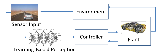
Figure 1: Automatic Emergency Braking System (AEBS) in closed loop. A machine learning based image classifier is used to perceive objects in the ego vehicle’s frame of view.

Example 1

As an illustrative example, let us consider a simple model of an Automatic Emergency Braking System (AEBS), that attempts to detect objects in front of a vehicle and actuate the brakes when needed to avert a collision. Figure 1 shows the AEBS as a system composed of a controller (automatic braking), a plant (vehicle sub-system under control, including transmission), and an advanced sensor (camera along with an obstacle detector based on deep learning). The AEBS, when combined with the vehicle’s environment, forms a closed loop control system. The controller regulates the acceleration and braking of the plant using the velocity of the subject (ego) vehicle and the distance between it and an obstacle. The sensor used to detect the obstacle includes a camera along with an image classifier based on deep neural networks. In general, this sensor can provide noisy measurements due to incorrect image classifications which in turn can affect the correctness of the overall system.

Suppose we want to verify whether the distance between the subject vehicle and a preceding obstacle is always larger than $\displaystyle 5$ meters. Such a verification requires the exploration of a very large input space comprising the control inputs (e.g., acceleration and braking pedal angles) and the ML component’s feature space (e.g., all the possible pictures observable by the camera). The latter space is particularly large — for example, note that the feature space of RGB images of dimension $\displaystyle 1000\times 600$px (for an image classifier) contains $\displaystyle 256^{1000\times 600\times 3}$ elements.

At first, the input space of the model described in Example 1 appears intractably large. However, the twin notions of abstraction and compositionality, central to much of the advances in formal verification, can help address this challenge. As mentioned earlier, we decompose the overall CPSML model input space into two parts: (i) the input space of the ML component, and (ii) the input space for the rest of the system – i.e., the CPSML model with an abstraction of the ML component. A CPS Analyzer operates on the latter “pure CPS” input space, while an ML Analyzer handles the former. The two analyzers communicate information as follows:

1. The CPS Analyzer initially performs conservative analyses assuming abstractions of the ML component. In particular, consider two extreme abstractions — a “perfect ML classifier” (i.e., all feature vectors are correctly classified), and a “completely-wrong ML classifier” (all feature vectors are misclassified). Abstraction permits the CPS Analyzer to operate on a lower-dimensional input space (the “pure CPS” one) and identify a region in this space that may be affected by the malfunctioning of some ML modules – a so-called “region of interest” or “region of uncertainty.” This region is communicated to the ML Analyzer.

2. The ML Analyzer projects the region of uncertainty (ROU) onto its input space, and performs a detailed analysis of that input sub-space. Since this detailed analysis uses only the ML classifier (not the full CPSML model), it is a more tractable problem. In this paper, we present a novel sampling-based approach to explore the input sub-space for the ML component. We can also leverage other advances in analysis of machine learning systems operating on rich sensor inputs and for applications such as autonomous driving (see the related work section that follows).

3. When the ML Analyzer finds interesting test cases (e.g., those that trigger misclassifications of inputs whose labels are easily inferred), it communicates that information back to the CPS Analyzer, which checks whether the ML misclassification can lead to a system-level safety violation (e.g., a collision). If yes, we have found a system-level counterexample. If not, the ROU is updated and the revised ROU passed back to the ML Analyzer.

The communication between the CPS Analyzer and ML Analyzer continues until either we find a system-level counterexample, or we run out of resources. For the class of CPSML models we consider, including those with highly non-linear dynamics and even black-box components, one cannot expect to prove system correctness. We focus on specifications in Signal Temporal Logic (STL), and for this reason use a temporal logic falsifier, Breach donze2010breach , as our CPS Analyzer; however, other specification formalisms and tools may also be used and our framework is largely agnostic to these choices. Even though temporal logic falsification is a mature technology with initial industrial adoption (e.g., yamaguchi-fmcad16 ), several technical challenges remain. First, we need to construct the validity domain of an STL specification — the input sub-space where the property is satisfied — for a CPSML model with abstracted (correct/incorrect) ML components, and identify the region of uncertainty (ROU). Second, we need a method to relate the ROU to the feature space of the ML modules. Third, we need to systematically analyze the feature space of the ML component with the goal of finding feature vectors leading to misclassifications. We describe in detail in Sections 3 and 4 how we tackle these challenges.

In summary, the main contributions of this paper are:

• A compositional framework for the falsification of temporal logic properties of arbitrary CPSML models that works for any kind of machine learning classifier. To our knowledge, we present the first approach to falsifying temporal logic properties of closed-loop CPS with ML components, including deep neural networks.

• The first approach for formal analysis of systems that use ML for perception. In particular, we show how to use a novel combination of abstraction and compositional reasoning to scale falsification to the higher-dimensional input spaces occurring for ML-based perception. Our compositional framework is the first modular approach to verification of CPSML, and the first to systematically deal with the specification challenge for ML-based perception as described in SeshiaS16 .

• A machine learning analyzer that identifies misclassifications leading to system-level property violations, based on the following main ideas:

  • An input space parameterization used to abstract the feature space of the ML component and relate it to the CPSML input space;

  • Systematic sampling methods to explore the feature space of the ML component, and

  • A classifier approximation method used to abstract the ML component and identify misclassifications that can lead to executions of the CPSML that violate the temporal logic specification (i.e., system-level counterexamples).

• An experimental demonstration of the effectiveness of our approach on two instantiations of an Automatic Emergency Braking System (AEBS) example with multiple deep neural networks trained for object detection and classification, including some developed by experts in the machine learning and computer vision communities.

In Sec. 5, we give detailed experimental results on an Automatic Emergency Braking System (AEBS) involving an image classifier for obstacle detection based on deep neural networks developed and trained using leading software packages — AlexNet developed with Caffe jia2014caffe and Inception-v3 developed with TensorFlow tensorflow2015 . In this journal version of our original conference paper dreossi-nfm17 , we also present a new case study, an AEBS deployed within the Udacity self-driving car simulator udacitySim-www trained on images generated from the simulator.

Related Work

The verification of both CPS and ML algorithms have attracted several research efforts, and we focus here on the most closely related work. Techniques for the falsification of temporal logic specifications against CPS models have been implemented based on nonlinear optimization methods and stochastic search strategies (e.g., Breach donze2010breach , S-TaLiRo annpureddyLFS11 , RRT-REX dreossi2015efficient , C2E2 duggirala2015c2e2 ). While the verification of ML programs is less well-defined SeshiaS16 , recent efforts szegedy2013intriguing show how even well trained neural networks can be sensitive to small adversarial perturbations, i.e., small intentional modifications that lead the network to misclassify the altered input with large confidence. Other efforts have tried to characterize the correctness of neural networks in terms of risk vapnik1991principles (i.e., probability of misclassifying a given input) or robustness fawzi2015analysis ; carlini-ieeesp17 (i.e., a minimal perturbation leading to a misclassification), while others proposed methods to generate pictures nguyen2015deep ; dreossi-rmlw17 or perturbations moosavi2015deepfool ; nguyen2015deep including methods based on satisfiability modulo theories (SMT) (e.g., huang-arxiv16 ) in such a way to “fool” neural networks. These methods, while very promising, are limited to analyzing partial specifications of the ML components in isolation, and not in the context of a complex, closed-loop cyber-physical system. To the best of our knowledge, our work is the first to address the verification of end-to-end temporal logic properties of CPSML—the combination of CPS and ML systems. The work that is closest in spirit to ours is that on DeepXplore pei-sosp17 , where the authors present a whitebox software testing approach for deep learning systems. However, there are some important differences: their work performs a detailed analysis of the learning software, whereas ours analyzes the entire closed-loop CPS while delegating the software analysis to the machine learning analyzer. Further, we consider temporal logic falsification whereas their work uses software and neural network coverage metrics. It may be interesting to see how these approaches can be combined. We believe our approach is the first step towards performing a more “semantic” adversarial analysis of systems that employ machine learning, including deep learning dreossi-cav18 .

2 Background

2.1 CPSML Models

In this work, we consider models of cyber-physical systems with machine learning components (CPSML). We assume that a system model is given as a gray-box simulator defined as a tuple $\displaystyle M=(S,U,sim)$, where $\displaystyle S$ is a set of system states, $\displaystyle U$ is a set of input values, and $\displaystyle sim:S\times U\times T\to S$ is a simulator that maps a state $\displaystyle\mathbf{s}(t_{k})\in S$ and input value $\displaystyle\mathbf{u}(t_{k})\in U$ at time $\displaystyle t_{k}\in T$ to a new state $\displaystyle\mathbf{s}(t_{k+1})=sim(\mathbf{s}(t_{k}),\mathbf{u}(t_{k}),t_{k})$, where $\displaystyle t_{k+1}=t_{k}+\Delta_{k}$ for a time-step $\displaystyle\Delta_{k}\in\mathbb{Q}_{>0}$.

Given an initial time $\displaystyle t_{0}\in T$, an initial state $\displaystyle\mathbf{s}(t_{0})\in S$, a sequence of time-steps $\displaystyle\Delta_{0},\dots,\Delta_{n}\in\mathbb{Q}_{>0}$, and a sequence of input values $\displaystyle\mathbf{u}(t_{0}),\dots,\mathbf{u}(t_{n})\in U$, a simulation trace of the model $\displaystyle M=(S,U,sim)$ is a sequence:

$$(t_{0},\mathbf{s}(t_{0}),\mathbf{u}(t_{0})),(t_{1},\mathbf{s}(t_{1}),\mathbf{u}(t_{1})),\dots,(t_{n},\mathbf{s}(t_{n}),\mathbf{u}(t_{n}))$$

where $\displaystyle\mathbf{s}(t_{k+1})=sim(\mathbf{s}(t_{k}),\mathbf{u}(t_{k}),\Delta_{k})$ and $\displaystyle t_{k+1}=t_{k}+\Delta_{k}$ for $\displaystyle k=0,\dots,n$.

The gray-box aspect of the CPSML model is that we assume some knowledge of the internal ML components. Specifically, these components, termed classifiers, are functions $\displaystyle f:X\to Y$ that assign to their input feature vector $\displaystyle\mathbf{x}\in X$ a label $\displaystyle y\in Y$, where $\displaystyle X$ and $\displaystyle Y$ are a feature and label space, respectively. Without loss of generality, we focus on binary classifiers whose label space is $\displaystyle Y=\{0,1\}$. An ML algorithm selects a classifier using a training set $\displaystyle\{(\mathbf{x}^{(1)},y^{(1)}),\dots,(\mathbf{x}^{(m)},y^{(m)})\}$ where the $\displaystyle(\mathbf{x}^{(i)},y^{(i)})$ are labeled examples with $\displaystyle\mathbf{x}^{(i)}\in X$ and $\displaystyle y^{(i)}\in Y$, for $\displaystyle i=1,\dots,m$. The quality of a classifier can be estimated on a test set of examples comparing the classifier predictions against the labels of the examples. Precisely, for a given test set $\displaystyle T=\{(\mathbf{x}^{(1)},y^{(1)}),\dots,(\mathbf{x}^{(l)},y^{(l)})\}$, the number of false positives $\displaystyle fp_{f}(T)$ and false negatives $\displaystyle fn_{f}(T)$ of a classifier $\displaystyle f$ on $\displaystyle T$ are defined as:

$$\begin{split}fp_{f}(T)=&\ \mid\{\mathbf{x}^{(i)}\in T\mid f(\mathbf{x}^{(i)})=1\text{ and }y^{(i)}=0\}\mid\\ fn_{f}(T)=&\ \mid\{\mathbf{x}^{(i)}\in T\mid f(\mathbf{x}^{(i)})=0\text{ and }y^{(i)}=1\}\mid\\ \end{split}$$ (1)

The error rate of $\displaystyle f$ on $\displaystyle T$ is given by:

$$err_{f}(T)=(fp_{f}(T)+fn_{f}(T))/l$$ (2)

A low error rate implies good predictions of the classifier $\displaystyle f$ on the test set $\displaystyle T$.

2.2 Signal Temporal Logic

We consider Signal Temporal Logic maler2004monitoring (STL) as the language to specify properties to be verified against a CPSML model. STL is an extension of linear temporal logic (LTL) suitable for the specification of properties of CPS.

A signal is a function $\displaystyle s:D\to S$, with $\displaystyle D\subseteq\mathbb{R}_{\geq 0}$ an interval and either $\displaystyle S\subseteq\mathbb{B}$ or $\displaystyle S\subseteq\mathbb{R}$, where $\displaystyle\mathbb{B}=\{\top,\bot\}$ and $\displaystyle\mathbb{R}$ is the set of reals. Signals defined on $\displaystyle\mathbb{B}$ are called booleans, while those on $\displaystyle\mathbb{R}$ are said real-valued. A trace $\displaystyle w=\{s_{1},\dots,s_{n}\}$ is a finite set of real-valued signals defined over the same interval $\displaystyle D$.

Let $\displaystyle\Sigma=\{\sigma_{1},\dots,\sigma_{k}\}$ be a finite set of predicates $\displaystyle\sigma_{i}:\mathbb{R}^{n}\to\mathbb{B}$, with $\displaystyle\sigma_{i}\equiv p_{i}(x_{1},\dots,x_{n})\lhd 0$, $\displaystyle\lhd\in\{<,\leq\}$, and $\displaystyle p_{i}:\mathbb{R}^{n}\to\mathbb{R}$ a function in the variables $\displaystyle x_{1},\dots,x_{n}$.

An STL formula is defined by the following grammar:

$$\varphi:=\sigma\,|\,\neg\varphi\,|\,\varphi\wedge\varphi\,|\,\varphi U_{I}\varphi$$ (3)

where $\displaystyle\sigma\in\Sigma$ is a predicate and $\displaystyle I\subset\mathbb{R}_{\geq 0}$ is a closed non-singular interval. Other common temporal operators can be defined as syntactic abbreviations in the usual way, like for instance $\displaystyle\varphi_{1}\vee\varphi_{2}:=\neg(\neg\varphi_{1}\wedge\varphi_{2})$, $\displaystyle F_{I}\varphi:=\top U_{I}\varphi$, or $\displaystyle G_{I}\varphi:=\neg F_{I}\neg\varphi$. Given a $\displaystyle t\in\mathbb{R}_{\geq 0}$, a shifted interval $\displaystyle I$ is defined as $\displaystyle t+I=\{t+t^{\prime}\mid t^{\prime}\in I\}$.

Definition 1 (Qualitative semantics)

Let $\displaystyle w$ be a trace, $\displaystyle t\in\mathbb{R}_{\geq 0}$, and $\displaystyle\varphi$ be an STL formula. The qualitative semantics of $\displaystyle\varphi$ is inductively defined as follows:

$$\begin{split}w,t\models\sigma\text{ iff }&\sigma(w(t))\text{ is true}\\ w,t\models\neg\varphi\text{ iff }&w,t\not\models\varphi\\ w,t\models\varphi_{1}\wedge\varphi_{2}\text{ iff }&w,t\models\varphi_{1}\text{ and }w,t\models\varphi_{2}\\ w,t\models\varphi_{1}U_{I}\varphi_{2}\text{ iff }&\exists t^{\prime}\in t+I\text{ s.t. }w,t^{\prime}\models\varphi_{2}\text{ and }\forall t^{\prime\prime}\in[t,t^{\prime}],w,t^{\prime\prime}\models\varphi_{1}\\ \end{split}$$ (4)

A trace $\displaystyle w$ satisfies a formula $\displaystyle\varphi$ if and only if $\displaystyle w,0\models\varphi$, in short $\displaystyle w\models\varphi$. For given signal $\displaystyle w$, time instant $\displaystyle t\in\mathbb{R}_{\geq 0}$, and STL formula $\displaystyle\varphi$, the satisfaction signal $\displaystyle\mathcal{X}(w,t,\varphi)$ is $\displaystyle\top$ if $\displaystyle w,t\models\varphi$, $\displaystyle\bot$ otherwise.

Given a CPSML model $\displaystyle M=(S,U,sim)$, $\displaystyle M\models\varphi$ if every simulation trace of $\displaystyle M$ satisfies $\displaystyle\varphi$.

Definition 2 (Quantitative semantics)

Let $\displaystyle w$ be a trace, $\displaystyle t\in\mathbb{R}_{\geq 0}$, and $\displaystyle\varphi$ be an STL formula. The quantitative semantics of $\displaystyle\varphi$ is defined as follows:

$$\begin{split}\rho(p(x_{1},\dots,x_{n})\lhd 0,w,t)=&\ p(w(t))\text{ with }\lhd\in\{<,\leq\}\\ \rho(\neg\varphi,w,t)=&\ -\rho(\varphi,w,t)\\ \rho(\varphi_{1}\wedge\varphi_{2},w,t)=&\ \min(\rho(\varphi_{1},w,t),\rho(\varphi_{2},w,t))\\ \rho(\varphi_{1}U_{I}\varphi_{2},w,t)=&\ \sup_{t^{\prime}\in t+I}\min(\rho(\varphi_{2},w,t^{\prime}),\inf_{t^{\prime\prime}[t,t^{\prime}]}\rho(\varphi_{1},w,t^{\prime\prime}))\\ \end{split}$$ (5)

The robustness of a formula $\displaystyle\varphi$ with respect to a trace $\displaystyle w$ is the signal $\displaystyle\rho(\varphi,w,\cdot)$.

Quantitative semantics helps to determine how robustly a formula is satisfied. Intuitively, the quantitative evaluation of a formula provides a real value representing the distance to satisfaction or violation. The quantitative and qualitative semantics are connected. Specifically, it holds that $\displaystyle\rho(\varphi,w,t)>0$ if and only if $\displaystyle w,t\models\varphi$ donze2013efficient .

Given a CPSML model $\displaystyle M=(S,U,sim)$, and a temporal logic formula $\displaystyle\varphi$, the validity domain of $\displaystyle\varphi$ for model $\displaystyle M$ is the subset of $\displaystyle U$ for which traces of $\displaystyle M$ satisfy $\displaystyle\varphi$. We denote the validity domain by $\displaystyle U_{\varphi}$; the remaining set of inputs $\displaystyle U\setminus U_{\varphi}$ is denoted by $\displaystyle U_{\neg\varphi}$. Note that there are no limitations on the dimensionality of a validity domain. It can potentially characterize single initial conditions as well as entire input traces. Usually when we speak of validity domains as sets of traces, we represent them using a suitable finite parameterization of traces. Simulation-based verification tools (such as donze2010breach ) can approximately compute validity domains via sampling-based methods.

3 Compositional Falsification Framework

In this section, we formalize the falsification problem for STL specifications against CPSML models, define our compositional falsification framework, and show its functionality on the AEBS system of Example 1.

Definition 3 (Falsification of CPSML)

Given a model $\displaystyle M=(S,U,sim)$ and an STL specification $\displaystyle\varphi$, find an initial state $\displaystyle\mathbf{s}(t_{0})\in S$ and a sequence of input values $\displaystyle\mathbf{u}=\mathbf{u}(t_{0}),\dots,\mathbf{u}(t_{n})\in U$ such that the trace of states $\displaystyle w=\mathbf{s}(t_{0}),\dots,\mathbf{s}(t_{n})$ generated by the simulation of $\displaystyle M$ from $\displaystyle\mathbf{s}(t_{0})\in S$ under $\displaystyle\mathbf{u}$ does not satisfy $\displaystyle\varphi$, i.e., $\displaystyle w\not\models\varphi$. We refer to such $\displaystyle(\mathbf{s}(t_{0}),\mathbf{u})$ as counterexamples for $\displaystyle\varphi$. The problem of finding a counterexample is often called the falsification problem.

We now present the compositional framework for the falsification of STL formulas against CPSML models. Intuitively, the proposed method decomposes a given model into two parts: (i) an abstraction of the CPSML model under the assumption of perfectly correct ML modules, and (ii) its actual ML components. The two parts are separately analyzed, the first by a temporal logic falsifier that builds the validity domain with respect to the given specification, the second by an ML analyzer that identifies sets of feature vectors that are misclassified by the ML components. Finally, the results of the two analyses are composed and projected back to a targeted input subspace of the original CPSML model where counterexamples can be found by invoking a temporal logic falsifier. We next formalize this procedure.

Let $\displaystyle M=(S,U,sim)$ be a CPSML model and $\displaystyle\varphi$ be an STL specification. $\displaystyle U_{\varphi}$ is the validity domain of $\displaystyle\varphi$ for $\displaystyle M$. Thus, for falsification, we wish to find an element of $\displaystyle U_{\neg\varphi}$. The challenge is that the dimensionality of the input space $\displaystyle U$ is very high.

We address this challenge through a combination of abstraction and compositional reasoning. Consider creating an “optimistic” abstraction $\displaystyle M^{+}$ of $\displaystyle M$: in other words, $\displaystyle M^{+}$ is a version of $\displaystyle M$ with perfect ML components, that is, every feature vector of the ML feature space is correctly classified. Let us denote by $\displaystyle ml$ the unabstracted ML components of the model $\displaystyle M$.

Under the assumption of correct ML components, the lower-dimensional input space of $\displaystyle M^{+}$ can be analyzed by constructing the validity domain of $\displaystyle\varphi$, that is the partition of the input space of $\displaystyle M^{+}$ into the sets $\displaystyle U_{\varphi}^{+}$ and $\displaystyle U_{\neg\varphi}^{+}$ that do and do not satisfy $\displaystyle\varphi$, respectively. The set $\displaystyle U_{\neg\varphi}^{+}$ comprises inputs on which the CPSML model violates $\displaystyle\varphi$ even if the ML component operates perfectly, i.e., the system perceives its environment perfectly. For falsification, we are interested in identifying points in $\displaystyle U_{\varphi}^{+}$ that correspond to environments in which a misclassification produced by $\displaystyle ml$ can result in $\displaystyle M$ violating $\displaystyle\varphi$. This corresponds to analyzing the behavior of the ML components $\displaystyle ml$ on inputs corresponding to the set $\displaystyle U_{\varphi}^{+}$. We refer to this step as the ML analysis. It can be seen as a procedure for finding a subset $\displaystyle U^{ml}\subseteq U$ of input values mapping to feature vectors that are misclassified by the ML components $\displaystyle ml$. It is important to note that the input space of the CPS model $\displaystyle M^{+}$ and the feature spaces of the ML modules $\displaystyle ml$ are different; thus, the ML analyzer must adapt and relate the two different spaces. This important step will be clarified in Section 4.

Finally, the set $\displaystyle U^{ml}$ generated by the decomposed analysis of the CPS model and its ML components targets a small set of input values that are misclassified by the ML modules and are likely to falsify $\displaystyle\varphi$. Thus, system-level counterexamples in $\displaystyle U^{ml}\subseteq U$ can be determined by invoking a temporal logic falsifier on $\displaystyle\varphi$ against the original model $\displaystyle M$.

As explained below, we can pair the “optimistic” abstraction explained above with a “pessimistic” abstraction as well, so as to obtain a further restriction of the input space.

Algorithm 1 CPSML falsification scheme (one iteration between CPS Analyzer and ML Analyzer)

1:function CompFalsfy($\displaystyle M,\varphi$)$\displaystyle\triangleright$ $\displaystyle M$ CPSML, $\displaystyle\varphi$ STL specification

2:     $\displaystyle[M^{+},ml]\leftarrow$Decompose($\displaystyle M$)$\displaystyle\triangleright$ $\displaystyle M^{+}$ – perfect ML, $\displaystyle ml$ – ML component

3:     $\displaystyle[U_{\varphi}^{+},U_{\neg\varphi}^{+}]\leftarrow$ValidityDomain($\displaystyle M^{+},U,\varphi$)$\displaystyle\triangleright$ Validity domain of $\displaystyle\varphi$ w.r.t. $\displaystyle M^{+}$

4:     $\displaystyle[M^{-},ml]\leftarrow$Decompose($\displaystyle M$)$\displaystyle\triangleright$ $\displaystyle M^{-}$ – wrong ML, $\displaystyle ml$ – ML component

5:     $\displaystyle[U_{\varphi}^{-},U_{\neg\varphi}^{-}]\leftarrow$ValidityDomain($\displaystyle M^{-},U,\varphi$)$\displaystyle\triangleright$ Validity domain of $\displaystyle\varphi$ w.r.t. $\displaystyle M^{-}$

6:     $\displaystyle U_{rou}\leftarrow U_{\varphi}^{+}\setminus U_{\varphi}^{-}$ $\displaystyle\triangleright$ Compute ROU

7:     $\displaystyle U^{ml}\leftarrow$ MLAnalysis($\displaystyle ml,U_{rou}$)$\displaystyle\triangleright$ Find misclassified feature vectors in ROU

8:     $\displaystyle U^{ml}_{\neg\varphi}\leftarrow$Falsify($\displaystyle M,U^{ml},\varphi$)$\displaystyle\triangleright$ Falsify property on original model with targeted inputs

9:     return $\displaystyle U_{\neg\varphi}^{+}\cup U^{ml}_{\neg\varphi}$

10:end function

The compositional falsification procedure is formalized in Algorithm 1 which shows one iteration of creating abstractions, calling the CPS falsifier, and the ML analyzer. Figure 2 shows the overall procedure which includes Algorithm 1. CompFalsfy receives as input a CPSML model $\displaystyle M$ and an STL specification $\displaystyle\varphi$, and returns a set of falsifying counterexamples. At first, the algorithm decomposes $\displaystyle M$ into $\displaystyle M^{+}$ and $\displaystyle ml$, where $\displaystyle M^{+}$ is an abstract version of $\displaystyle M$ with ML components $\displaystyle ml$ that return perfect answers (classifications) (Line 2). Then, the validity domain of $\displaystyle\varphi$ with respect to the abstraction $\displaystyle M^{+}$ is computed by ValidityDomain (Line 3). Next, the algorithm computes $\displaystyle M^{-}$ and $\displaystyle ml$ from $\displaystyle M$, where $\displaystyle M^{-}$ is an abstract version of $\displaystyle M$ with ML components $\displaystyle ml$ that always return wrong answers (misclassifications) (Line 4). Note that this step can be combined with Line 2, but we leave it separate for clarity in the abstract algorithm specification. Then, the validity domain of $\displaystyle\varphi$ with respect to the abstraction $\displaystyle M^{-}$ is computed by ValidityDomain (Line 5). The region of uncertainty (ROU), where misclassifications of the ML components can lead to violations of $\displaystyle\varphi$, is then computed as $\displaystyle U_{rou}$ (Line 6). From this, the subset of inputs to the CPSML model that are misclassified by $\displaystyle ml$ is identified by MLAnalysis (Line 7). Finally, the targeted input set $\displaystyle U^{ml}$, comprising the intersection of the sets identified by the decomposed analysis, is searched by a temporal logic falsifier on the original model $\displaystyle M$ (Line 8) and the set of inputs that falsify the temporal logic formula are returned. It is important to note that the counterexamples we generate are for the concrete CPSML model $\displaystyle M$, i.e., the one with the actual ML component, not its optimistic or pessimistic abstraction.

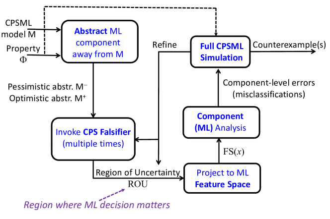
Figure 2: Compositional Falsification Technique. The method combines abstraction of the ML component with temporal logic falsification of the abstracted system and analysis of the ML component.

Note that the above approach can be implemented even without computing $\displaystyle M^{-}$ (Lines 4-6), in which case the entire validity domain of $\displaystyle\varphi$ is considered as the ROU. For simplicity, we will take this truncated approach in the example described below. In Section 5, we will describe results on the AEBS case study with the full approach.

Figure 3: Compositional falsification scheme on AEBS model. The “score” indicates the confidence level with which the classifier determines whether the image contains a car or not.

Example 2

Let us consider the model described in Example 1 and let us assume that the concrete input space $\displaystyle U$ of the CPSML model $\displaystyle M$ consists of the initial velocity of the subject vehicle $\displaystyle vel(0)$, the initial distance between the vehicle and the preceding obstacle $\displaystyle dist(0)$, and the sequence of pictures that can be captured by the camera. Let $\displaystyle\varphi:=G_{[0,T]}(dist(t)\geq\tau)$ be a specification that requires the vehicle to be always farther than $\displaystyle\tau$ from the preceding obstacle. Instead of analyzing the whole input space $\displaystyle U$ (including a vast number of pictures), we adopt our compositional framework to target a specific subset of $\displaystyle U$. Let $\displaystyle M^{+}$ be the optimistic abstraction of the AEBS model, i.e., assuming a perfectly working image classifier, and let $\displaystyle ml$ be the actual classifier. We begin by computing the validity subsets $\displaystyle U_{\varphi}^{+}$ and $\displaystyle U_{\neg\varphi}^{+}$ of $\displaystyle\varphi$ against $\displaystyle M^{+}$, considering only $\displaystyle vel(0)$ and $\displaystyle dist(0)$ and assuming exact distance measurements during the simulation. Next, we analyze only the image classifier $\displaystyle ml$ on pictures of obstacles whose distances fall in $\displaystyle U_{\varphi}^{+}$, say in a range $\displaystyle[d_{m},d_{M}]$ (see Figure 3). Our ML analyzer generates only pictures of obstacles whose distances are in $\displaystyle[d_{m},d_{M}]$, finds possible sets of images that are misclassified, and returns the corresponding distances that, when projected back to $\displaystyle U$, yields the subset $\displaystyle U^{ml}$ of $\displaystyle U$. Finally, a temporal logic falsifier can be invoked to search over the restricted input space $\displaystyle U^{ml}$ and a set of counterexamples is returned.

Algorithm 1 and the above example show how our compositional approach relies on three key steps: (i) computing the validity domain for an STL formula for a given simulation model; (ii) falsifying an STL formula on a simulation model, and (iii) a ML analyzer that computes a sub-space of its input feature space that leads to misclassifications. The first two steps have been well-studied in the literature on simulation-based verification of CPS, and implemented in tools such as Breach donze2010breach . We discuss our approach to Step (iii) in the next section — our ML analyzer that identifies misclassifications of the ML component relevant to the overall CPSML input space.

4 Machine Learning Analyzer

A central idea in our approach to analyzing CPSML models is to use abstractions of the ML components. For instance, in the preceding section, we used the notions of perfect ML classifiers and always-wrong classifiers in computing the region of uncertainty (ROU). In this section, we extend this abstraction-based approach to the ML classifier and its input (feature) space.

One motivation for our approach comes from the application domain of autonomous driving where machine learning is used for object detection and perception. Instead of exploring the high-dimensional input space for the ML classifier involving all combinations of pixels, we instead perform the key simplification of exploring realistic and meaningful modifications to a given image dataset that corresponds to the ROU. Autonomous driving groups spend copious amounts of time collecting images and video to train their learning-based perception systems with. We focus on analyzing the space of images that is “close” to this data set but with semantically significant modifications that can identify problematic cases for the overall system.

The space of modifications to input feature vectors (say, images) induces an abstract space over the concrete feature (image) space. Let us denote the abstract input domain by $\displaystyle A$. Given a classifier $\displaystyle f:X\to Y$, our ML analyzer computes a simpler function $\displaystyle\tilde{f}:A\to Y$ that approximates $\displaystyle f$ on the abstract domain $\displaystyle A$. The abstract domain of the function $\displaystyle\tilde{f}$ is analyzed and clusters of misclassifying abstract elements are identified. The concretizations of such elements are subsets of features that are misclassified by the original classifier $\displaystyle f$. We describe further details of this approach in the remainder of this section.

4.1 Feature Space Abstraction

Let $\displaystyle\tilde{X}\subseteq X$ be a subset of the feature space of $\displaystyle f:X\to Y$. Let $\displaystyle\leq$ be a total order on a set $\displaystyle A$ called the abstract set. An abstraction function is an injective function $\displaystyle\alpha:\tilde{X}\to A$ that maps every feature vector $\displaystyle\mathbf{x}\in\tilde{X}$ to an abstract element $\displaystyle\alpha(\mathbf{x})\in A$. Conversely, the concretization function $\displaystyle\gamma:A\to\tilde{X}$ maps every abstraction $\displaystyle\mathbf{a}\in A$ to a feature $\displaystyle\gamma(\mathbf{a})\in\tilde{X}$.

The abstraction and concretization functions play a fundamental role in our falsification framework. First, they allow us to map the input space of the CPS model to the feature space of its classifiers. Second, the abstract space can be used to analyze the classifiers on a compact domain as opposite to intractable feature spaces. These concepts are clarified in the following example, where a feature space of pictures is abstracted into a three-dimensional unit hyper-box.

Example 3

Let $\displaystyle X$ be the set of RGB pictures of size $\displaystyle 1000\times 600$, i.e., $\displaystyle X=\{0,\dots,255\}^{1000\times 600\times 3}$. Suppose we are interested in analyzing a ML image classifier in the context of our AEBS system. In this case, we are interested in images of road scenarios rather than on arbitrary images in $\displaystyle X$. Further, assume that we start with a reference data set of images of a car on a two-lane highway with a desert road background, as shown in Figure 4. Suppose that we are interested only in the constrained feature space $\displaystyle\tilde{X}\subseteq X$ comprising this desert road scenario with a single car on the highway and three dimensions along which the scene can be varied: (i) the x-dimension (lateral) position of the car; (ii) the z-dimension (distance from the sensor) position of the car, and (iii) the brightness of the image. The $\displaystyle x$ and $\displaystyle z$ positions of the car and the brightness level of the picture can be seen as the dimensions of an abstract set $\displaystyle A$. In this setting, we can define the abstraction and concretization functions $\displaystyle\alpha$ and $\displaystyle\gamma$ that relate the abstract set $\displaystyle A=[0,1]^{3}$ and $\displaystyle\tilde{X}$. For instance, the picture $\displaystyle\gamma(0,0,0)$ sees the car on the left, close to the observer, and low brightness; the picture $\displaystyle\gamma(1,0,0)$ places the car shifted to the right; on the other extreme, $\displaystyle\gamma(1,1,1)$ has the car on the right, far away from the observer, and with a high brightness level. Figure 4 depicts some car pictures of $\displaystyle\tilde{S}$ disposed accordingly to their position in the abstract domain $\displaystyle A$ (the surrounding box).

Figure 4: Feature Space Abstraction. The cube represents the abstract space $\displaystyle A$ with the three dimensions corresponding to three different image modifications. The displayed road images correspond to concretized elements of the concrete feature space $\displaystyle\tilde{X}$.

4.2 Approximation of Learning Components

We now describe how the feature space abstraction can be used to construct an approximation that helps the identification of misclassified feature vectors.

Given a classifier $\displaystyle f:X\to Y$ and a constrained feature space $\displaystyle\tilde{X}\subseteq X$, we want to determine an approximated classifier $\displaystyle\tilde{f}:A\to Y$, such that $\displaystyle err_{\tilde{f}}(T)\leq\epsilon$, for some $\displaystyle 0\leq\epsilon\leq 1$ and test set $\displaystyle T=\{(\mathbf{a}^{(1)},y^{(1)}),\dots,(\mathbf{a}^{(l)},y^{(l)})\}$, with $\displaystyle y^{(i)}=f(\gamma(\mathbf{a}^{(i)}))$, for $\displaystyle i=1,\dots,l$.

Intuitively, the proposed approximation scheme samples elements from the abstract set, computes the labels of the concretized elements using the analyzed learning algorithm, and finally, interpolates the abstract elements and the corresponding labels in order to obtain an approximation function. Constructing such an approximation has multiple uses: (i) The process of finding a good approximation of $\displaystyle f$ appears to drive the sampling of elements towards misclassifications that lead to system-level counterexamples, and (ii) the obtained approximation $\displaystyle\tilde{f}$ can be used to perform higher-level analysis of the reason for misclassifications, e.g., by identifying clusters of misclassified feature vectors that share common characteristics. We elaborate on these aspects later in this section.

Algorithm 2 Approximation construction of classifier $\displaystyle f:X\to Y$

1:function Approximation($\displaystyle A,\gamma,\epsilon$)$\displaystyle\triangleright$ $\displaystyle A$ abstract set ($\displaystyle\gamma:A\to\tilde{X}$), $\displaystyle 0\leq\epsilon\leq 1$

2:     $\displaystyle T_{I}\leftarrow\emptyset$

3:     repeat

4:         $\displaystyle T_{I}\leftarrow T_{I}\cup$ sample($\displaystyle A,f$)

5:         $\displaystyle\tilde{f}\leftarrow$ interpolate($\displaystyle T_{I}$)

6:         $\displaystyle T_{E}\leftarrow$ sample($\displaystyle A,f$)

7:     until $\displaystyle err_{\tilde{f}}(T_{E})\leq\epsilon$

8:     return $\displaystyle\tilde{f}$

9:end function

The Approximation algorithm (Algorithm 2) formalizes the proposed approximation construction technique. It receives in input an abstract domain $\displaystyle A$ for the concretization function $\displaystyle\gamma:A\to\tilde{X}$, with $\displaystyle\tilde{X}\subseteq X$, the error threshold $\displaystyle 0\leq\epsilon\leq 1$, and returns a function $\displaystyle\tilde{f}:A\to Y$ that approximates $\displaystyle f$ on the constrained feature space $\displaystyle\tilde{X}$. The algorithm consists of a loop that iteratively improves the approximation $\displaystyle\tilde{f}$. At every iteration, the algorithm populates the interpolation test set $\displaystyle T_{I}$ by sampling abstract features from $\displaystyle A$ and computing the concretized labels according to $\displaystyle f$ (Line 4), i.e., sample($\displaystyle A,f$)$\displaystyle=\{(\mathbf{a},y)\mid\mathbf{a}\in\tilde{A},y=f(\gamma(\mathbf{a}))\}$, where $\displaystyle\tilde{A}\subseteq A$ is a finite subset of samples determined with some sampling method. Next, the algorithm interpolates the points of $\displaystyle T_{I}$ (Line 5) according to a suitably-chosen interpolation technique. The result is a function $\displaystyle\tilde{f}:A\to Y$ that simplifies the original classifier $\displaystyle f$ on the concretized constrained feature space $\displaystyle\tilde{X}$. The approximation is evaluated on the test set $\displaystyle T_{E}$. Note that at each iteration, $\displaystyle T_{E}$ changes while $\displaystyle T_{I}$ incrementally grows. The algorithm iterates until the error rate $\displaystyle err_{\tilde{f}}(T_{E})$ is smaller than the desired threshold $\displaystyle\epsilon$ (Line 7). This is a heuristic function approximation method, and there is no formal guarantee on termination of the loop; however, in practice, we have found that the loop always terminates with the desired error less than $\displaystyle\epsilon$.

The technique with which the samples in $\displaystyle T_{E}$ and $\displaystyle T_{I}$ are selected strongly influences the accuracy of the approximation. A good sampling method can find corner-case misclassifications and provide better high-level insight into the regions of the abstract space where $\displaystyle f$ generates misclassifications. In order to have a good coverage of the abstract set $\displaystyle A$, we propose the usage of low-discrepancy sampling methods that, differently from uniform random sampling, cover sets quickly and evenly. In this work, we use the Halton and lattice sequences, two common and easy-to-implement sampling methods, which we explain next.

4.3 Sampling Methods

Discrepancy is a notion from equidistribution theory weyl1916gleichverteilung ; rosenblatt1995pointwise that finds application in quasi-Monte Carlo techniques for error estimation and approximating the mean, standard deviation, integral, global maxima and minima of complicated functions, such as, e.g., our classification functions.

Definition 4 (Discrepancy morokoff1994quasi )

Let $\displaystyle X=\{\mathbf{x}^{(1)},\dots,\mathbf{x}^{(m)}\}$ be a finite set of points in $\displaystyle n$-dimensional unit space, i.e., $\displaystyle X\subset[0,1]^{n}$. The discrepancy of $\displaystyle X$ is given by:

$$D(X)=\sup_{B\in J}\mid\frac{\#(X,B)}{m}-vol(B)\mid$$ (6)

where $\displaystyle\#(X,B)=|\{\mathbf{x}\in X\mid\mathbf{x}\in B\}|$, i.e., the number of points in $\displaystyle X$ that fall in $\displaystyle B$, $\displaystyle vol(B)$ is the $\displaystyle n$-dimensional volume of $\displaystyle B$, and $\displaystyle J$ is the set of boxes of the form $\displaystyle\{\mathbf{x}\in\mathbb{R}^{n}|a_{i}\leq\mathbf{x}_{i}\leq b_{i}\}$, where $\displaystyle i=1,\dots,n$ and $\displaystyle 0\leq a_{i}<b_{i}<1$.

Definition 5 (Low-discrepancy sequence morokoff1994quasi )

A low-discrepancy sequence, also called quasi-random sequence, is a sequence with the property that for all $\displaystyle m\in\mathbb{N}$, its subsequence $\displaystyle X=\{\mathbf{x}^{(1)},\dots,\mathbf{x}^{(m)}\}$ has low discrepancy.

Low-discrepancy sequences fill spaces more uniformly than uncorrelated random points. This property makes low-discrepancy sequences suitable for problems where grids are involved, but it is unknown in advance how fine the grid must be to attain precise results. A low-discrepancy sequence can be stopped at any point where convergence is observed, whereas the usual uniform random sampling technique requires a large number of computations between stopping points trandafir_quasirandom . Low-discrepancy sampling methods have improved computational techniques in many areas, including robotics branicky2001quasi , image processing hannaford1993resolution , computer graphics shirley1991discrepancy , numerical integration sloan1994lattice , and optimization niederreiter1992random .

We now introduce two low-discrepancy sequences that will be used in this work. For more sequences and details see, e.g., niederreiter1988low .

1. Halton sequence morokoff1994quasi . Based on the choice of an arbitrary prime number $\displaystyle p$, the $\displaystyle i$-th sample is obtained by representing $\displaystyle i$ in base $\displaystyle p$, reversing its digits, and moving the decimal point by one position. The resulting number is the $\displaystyle i$-th sample in base $\displaystyle p$. For the multi-dimensional case, it is sufficient to choose a different prime number for each dimension. In practice, this procedure corresponds to choosing a prime base $\displaystyle p$, dividing the $\displaystyle[0,1]$ interval in $\displaystyle p$ segments, then $\displaystyle p^{2}$ segments, and so on.

2. Lattice sequence matousek2009geometric . A lattice can be seen as the generalization of a multi-dimensional grid with possibly nonorthogonal axes. Let $\displaystyle\alpha_{1},\dots,\alpha_{n-1}\in\mathbb{R}_{>0}$ be irrational numbers and $\displaystyle m\in\mathbb{N}$. The $\displaystyle i$-th sample of a lattice sequence is $\displaystyle(i/m,\{i\alpha_{1}\},\dots,\{i\alpha_{n-1}\})$, where the curly braces $\displaystyle\{\cdot\}$ denote the fractional part of the real value (modulo-one arithmetic).

Example 4

We now analyze two Convolutional Neural Networks (CNNs): the Caffe jia2014caffe version of AlexNet krizhevsky2012imagenet and the Inception-v3 model of Tensorflow tensorflow2015 , both trained on the ImageNet database imagenet . We sample $\displaystyle 1000$ points from the abstract domain defined in Example 3 using the lattice sampling techniques. These points encode the $\displaystyle x$ and $\displaystyle z$ displacements of a car in a picture and its brightness level (see Figure 4). Figure 5 (a) depicts the sampled points with their concretized labels. The green circles indicate correct classifications, i.e., the classifier identified a car, the red circles denote misclassifications, i.e., no car detected. The linear interpolation of the obtained points leads to an approximation function. The error rates $\displaystyle err_{\tilde{f}}(T_{E})$ of the obtained approximations (i.e., the discrepancies between the predictions of the original image classifiers and their approximations) computed on $\displaystyle 300$ randomly picked test cases are $\displaystyle 0.0867$ and $\displaystyle 0.1733$ for AlexNet and Inception-v3, respectively. Figure 5 (b) shows the projections of the approximation functions for the brightness value $\displaystyle 0.2$. The more red a region, the larger the sets of pictures for which the neural networks do not detect a car. For illustrative purposes, we superimpose the projections of Figure 5 (b) over the background used for the picture generation. These illustrations show the regions of the concrete feature vectors in which a vehicle is misclassified.

(a) Sampling.

(b) Interpolation projection.

(c) Feature space analysis.

Figure 5: ML analysis of AlexNet network developed with Caffe (top) and Inception-v3 network developed with Tensorflow (bottom) on a road scenario.

The analysis of Example 4 on AlexNet and Inception-v3 provides useful insights. First, we observe that Inception-v3 outperforms AlexNet on the considered road pictures since it correctly classifies more pictures than AlexNet. Second, we notice that AlexNet tends to correctly classify pictures in which the $\displaystyle x$ abstract component is either close to $\displaystyle 0$ or $\displaystyle 1$, i.e., pictures in which the car is not in the middle of the street, but on one of the two lanes. This suggests that the model might not have been trained enough with pictures of cars in the center of the road. Third, using the lattice method on Inception-v3, we were able to identify a corner case misclassification in a cluster of correct predictions (note the isolated red cross with coordinates $\displaystyle(0.1933,0.0244,0.4589)$). All this information provides insights on the classifiers that can be useful in the hunt for counterexamples.

5 Experimental Results

In this section we present two case studies, both involving an Automatic Emergency Braking System (AEBS), but differing in the details of the underlying simulator and controller. The first is a Simulink-based AEBS, the second is a Unity-Udacity simulator-based AEBS. The first case study showcases our full compositional falsification method based on abstraction and compositional reasoning. The second case study shows how we can apply falsification directly on the concrete CPSML model (i.e. without performing the optimistic/pessimistic abstractions of the neural network) while synthesizing sequences of images that lead to a system-level counterexample.

The falsification framework for the first case study has been implemented in a Matlab toolbox. The framework for the second case study has been written in Python and C#. Our tools deal with models of CPSML and STL specifications. They mainly consist of a temporal logic falsifier and an ML analyzer that interact to falsify the given STL specification against the decomposed models. As an STL falsifier, we chose the existing tool Breach donze2010breach , while the ML analyzer has been implemented from scratch. The main reason to choose Breach is that our system-level specification is in signal temporal logic, which is the requirement language underlying this tool. Further, it has been developed in our group at UC Berkeley, allowing for better integration with the other software components. We leverage both the qualitative and the quantitative semantics of Breach. The qualitative semantics is used to compute the validity domains of specifications used in our case studies. The quantitative semantics is used by Breach (and similar tools) to translate the STL formula into a cost function to be minimized so as to find a trace that drives its value below zero, i.e., a property violation. The ML analyzer implementation has two components: the feature space abstractor and the ML approximation algorithm (see Section 4). The feature space abstractor implements a scene generator that concretizes the abstracted feature vectors. The algorithm that computes an approximation of the analyzed ML component gives the user the option of selecting the sampling method and interpolation technique, as well as setting the desired error rate. Our tools are interfaced with the deep learning frameworks Caffe jia2014caffe and Tensorflow tensorflow2015 . We ran our tests on a desktop computer Dell XPS 8900, Intel (R) Core(TM) i7-6700 CPU 3.40GHz, DIMM RAM 16 GB 2132 MHz, GPUs NVIDIA GeForce GTX Titan X and Titan Xp, with Ubuntu 14.04.5 LTS and Matlab R2016b.

5.1 Case Study 1: Simulink-based AEBS

Our first case study is a closed-loop Simulink model of a semi-autonomous vehicle with an Advanced Emergency Braking System (AEBS) taeyoung2011development connected to a deep neural network-based image classifier. The model mainly consists of a four-speed automatic transmission controller linked to an AEBS that automatically prevents collisions with preceding obstacles and alleviates the harshness of a crash when a collision is likely to happen (see Figure 6).

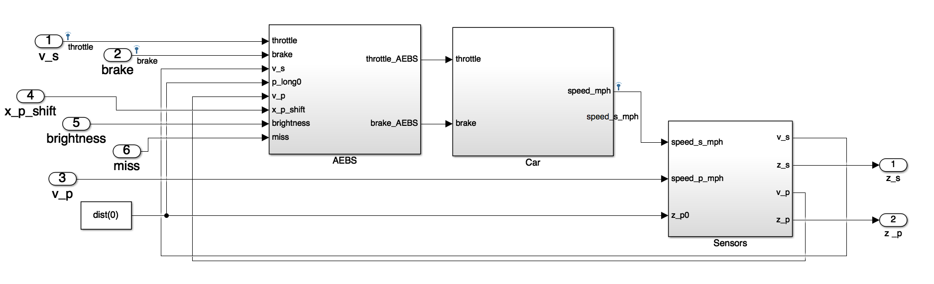
Figure 6: Simulink model of a semi-autonomous vehicle with AEBS.

The AEBS determines a braking mode depending on the speed of the vehicle $\displaystyle v_{s}$, the possible presence of a preceding obstacle, its velocity $\displaystyle v_{p}$, and the longitudinal distance $\displaystyle dist$ between the two. The distance $\displaystyle dist$ is provided by radars having $\displaystyle 30$m of range. For obstacles farther than $\displaystyle 30$m, the camera, connected to an image classifier, alerts the AEBS that, in the case of detected obstacle, goes into warning mode.

Depending on $\displaystyle v_{s},v_{p},dist$, and the presence of obstacles detected by the image classifier, the AEBS computes the time to collision and longitudinal safety indices, whose values determine a controlled transition between safe, warning, braking, and collision mitigation modes. In safe mode, the car does not need to brake. In warning mode, the driver should brake to avoid a collision. If this does not happen, the system goes into braking mode, where the automatic brake slows down the vehicle. Finally, in collision mitigation mode, the system, determining that a crash is unavoidable, triggers a full braking action aimed to minimize the damage.

To establish the correctness of the system and in particular of its AEBS controller, we formalize the STL specification $\displaystyle G(\neg(dist(t))\leq 0)$, that requires $\displaystyle dist(t)$ to always be positive, i.e., no collision happens. The input space is $\displaystyle v_{s}(0)\in[0,40]$ (mph), $\displaystyle dist(0)\in[0,60]$ (m), and the set of all RGB pictures of size $\displaystyle 1000\times 600$. The preceding vehicle is not moving, i.e., $\displaystyle v_{p}(t)=0$ (mph).

Figure 7: Validity domain for $\displaystyle G(\neg(dist(t))\leq 0)$ and AEBS model with different abstractions of ML component. The initial velocity and distance are on the x and y axes respectively. The dotted (horizontal) line is the image classifier activation threshold. Green indicates combinations of initial velocity and distance for which the property is satisfied and red indicates combinations for which the property is falsified. Our ML analyzer performs both optimistic (left) and pessimistic (middle) abstractions of the neural network classifier. On the right-most image, the yellow region denotes the region of uncertainty (ROU).

Figure 8: Analysis of Region of Uncertainty (ROU) for AEBS and property $\displaystyle G(\neg(dist(t))\leq 0)$. Red crosses in the ROU denote misclassifications generated by the ML analyzer that leads to a system-level counterexample. A circle denotes a “benign” misclassification.

At first, we compute the validity domain of $\displaystyle\varphi$ assuming that the radars are able to provide exact measurements for any distance $\displaystyle dist(t)$ and the image classifier correctly detects the presence of a preceding vehicle. The computed validity domain is depicted in Figure 7 (left-most image): green for $\displaystyle U_{\varphi}$ and red for $\displaystyle U_{\neg{\varphi}}$. Next, we try to identify candidate counterexamples that belong to the satisfactory set (i.e., the inputs that satisfy the specification) but might be influenced by a misclassification of the image classifier. Since the AEBS relies on the classifier only for distances larger than $\displaystyle 30$m, we can focus on the subset of the input space with $\displaystyle dist(0)\geq 30$. Specifically, we identify potential counterexamples by analyzing a pessimistic version of the model where the ML component always misclassifies the input pictures (see Figure 7, middle image). From these results, we can compute the region of uncertainty, shown in Figure 7 on the right. We can then focus our attention on the ROU, as shown in Fig. 8. In particular, we can identify candidate counterexamples, such as, for instance, $\displaystyle(25,40)$ (i.e., $\displaystyle v_{s}(0)=25$ and $\displaystyle dist(0)=40$).

Next, let us consider the AlexNet image classifier and the ML analyzer presented in Section 4 that generates pictures from the abstract feature space $\displaystyle A=[0,1]^{3}$, where the dimensions of $\displaystyle A$ determine the $\displaystyle x$ and $\displaystyle z$ displacements of a car and the brightness of a generated picture, respectively. The goal now is to determine an abstract feature $\displaystyle\mathbf{a}_{c}\in A$ related to the candidate counterexample $\displaystyle(25,40)$, that generates a picture that is misclassified by the ML component and might lead to a violation of the specification $\displaystyle\varphi$. The $\displaystyle dist(0)$ component of $\displaystyle\mathbf{u}_{c}=(25,40)$ determines a precise $\displaystyle z$ displacement $\displaystyle\mathbf{a}_{2}=0.2$ in the abstract picture. The connection between the abstract and input spaces is defined by the abstraction function that, in this case, was manually defined by the user. In general, this connection can be explicitly provided by a synthetic data generator such as, for instance, a simulator or image renderer. Now, we need to determine the values of the abstract $\displaystyle x$ displacement and brightness. Looking at the interpolation projection of Figure 5 (b), we notice that the approximation function misclassifies pictures with abstract component $\displaystyle\mathbf{a}_{1}\in[0.4,0.5]$ and $\displaystyle\mathbf{a}_{3}=0.2$. Thus, it is reasonable to try to falsify the original model on the input element $\displaystyle v_{s}(0)=25,dist(0)=40$, and concretized picture $\displaystyle\gamma(0.5,0.2,0.2)$. For this targeted input, the temporal logic falsifier computed a robustness value for $\displaystyle\varphi$ of $\displaystyle-24.60$, meaning that a falsifying counterexample has been found. Other counterexamples found with the same technique are, e.g., $\displaystyle(27,45)$ or $\displaystyle(31,56)$ that, associated with the correspondent concretized pictures with $\displaystyle\mathbf{a}_{1}=0.5$ and $\displaystyle\mathbf{a}_{3}=0.2$, lead to the robustness values $\displaystyle-23.86$ and $\displaystyle-24.38$, respectively (see Figure 8, red crosses). Conversely, we also disproved some candidate counterexamples, such as $\displaystyle(28,50)$, $\displaystyle(24,35)$, or $\displaystyle(25,45)$, whose robustness values are $\displaystyle 9.93,7.40$, and $\displaystyle 7.67$ (see Figure 8, green circles).

For experimental purposes, we try to falsify a counterexample in which we change the $\displaystyle x$ position of the abstract feature so that the approximation function correctly classifies the picture. For instance, by altering the counterexample $\displaystyle(27,45)$ with $\displaystyle\gamma(0.5,0.225,0.2)$ to $\displaystyle(27,45)$ with $\displaystyle\gamma(1.0,0.225,0.2)$, we obtain a robustness value of $\displaystyle 9.09$, that means that the AEBS is able to avoid the car for the same combination of velocity and distance of the counterexample, but different $\displaystyle x$ position of the preceding vehicle. Another example, is the robustness value $\displaystyle-24.38$ of the falsifying input $\displaystyle(31,56)$ with $\displaystyle\gamma(0.5,0.28,0.2)$, that altered to $\displaystyle\gamma(0.0,0.28,0.2)$, changes to $\displaystyle 12.41$.

Finally, we test Inception-v3 on the corner case misclassification identified in Section 4.2 (i.e., the picture $\displaystyle\gamma(0.1933,0.0244,0.4589)$). The distance $\displaystyle dist(0)=4.88$ related to this abstract feature is below the activation threshold of the image classifier. Thus, the falsification points are exactly the same as those of the computed validity domain (i.e., $\displaystyle dist(0)=4.88$ and $\displaystyle v_{s}(0)\in[4,40]$). This study shows how a misclassification of the ML component might not affect the correctness of the CPSML model.

5.2 Case Study 2: Unity-Udacity Simulator-based AEBS

We now analyze an AEBS deployed within Udacity’s self-driving car simulator. The simulator, built with the Unity game engine, can be used to teach cars how to navigate roads using deep learning. We modified the simulator in order to focus exclusively on the braking system. In our settings, the car steers by following some predefined waypoints, while acceleration and braking are controlled by an AEBS connected to a CNN. An onboard camera sends images to the CNN whose task is to detect cows on the road. Whenever an obstacle is detected, the AEBS triggers a brake that slows the vehicle down and prevents the collision against the obstacle.

We implemented a CNN that classifies the pictures captured by the onboard camera in two categories “cow” and “not cow”. The CNN has been implemented and trained using Tensorflow. We connected the CNN to the Unity C# class that controls the car. The communication between the neural network and the braking controller happens via Socket.IO protocol. A screenshot of the car braking in presence of a cow is shown in Figure 9a. A video of the AEBS in action can be seen at https://www.youtube.com/watch?v=Sa4oLGcHAhY.

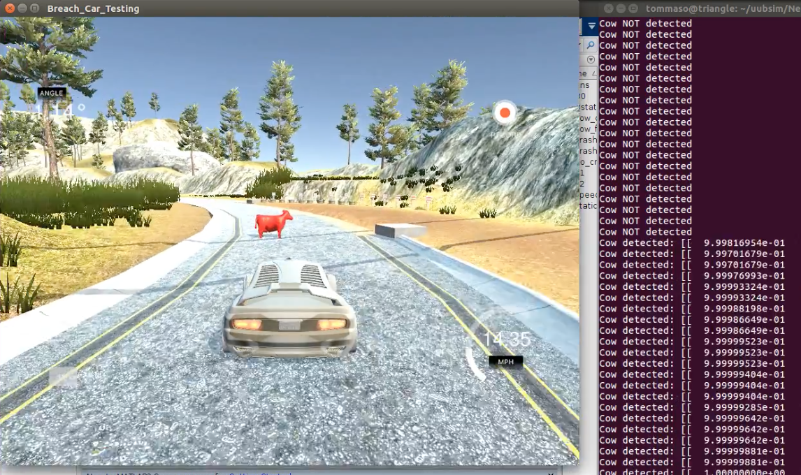
(a) Correct detection and braking.

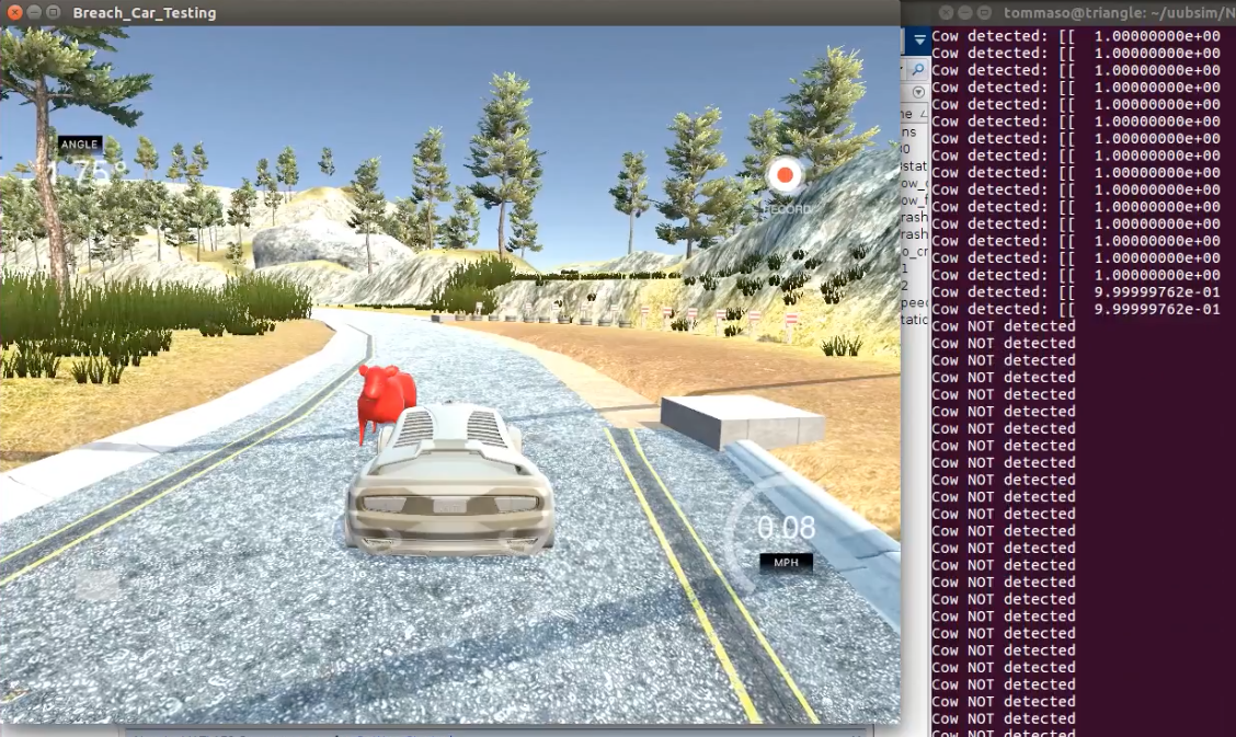
(b) Misclassification and collision.

Figure 9: Unity-Udacity simulator AEBS. The onboard camera sends images to the CNN. When a cow is detected a braking action is triggered until the car comes to a complete stop. Full videos available at https://www.youtube.com/watch?v=Sa4oLGcHAhY and https://www.youtube.com/watch?v=MaRoU5OgimE.

The CNN architecture is depicted in Figure 10. The network consists of eight layers: the first six are alternations of convolutions and max-pools with ReLU activations, the last two are a fully connected layer and a softmax that outputs the network prediction. The dimensions and hyperparameters of our neural network are shown in Table 1, where $\displaystyle l$ is a layer, $\displaystyle n_{H}^{[l]}\times n_{W}^{[l]}\times n_{C}^{[l]}$ is the dimension of the volume computed by the layer $\displaystyle l$, $\displaystyle f^{[l]}$ is the filter size, $\displaystyle p^{[l]}$ is the padding, and $\displaystyle s^{[l]}$ is the stride.

Figure 10: CNN architecture.

	0	1	2	3	4	5	6	7	8
$\displaystyle n_{H}^{[l]}\times n_{W}^{[l]}$	$\displaystyle 128\times 128$	$\displaystyle 128\times 128$	$\displaystyle 64\times 64$	$\displaystyle 64\times 64$	$\displaystyle 32\times 32$	$\displaystyle 32\times 32$	$\displaystyle 16\times 16$	$\displaystyle 128\times 1$	$\displaystyle 2\times 1$
$\displaystyle n_{C}^{[l]}$	3	32	32	32	32	64	64	1	1
$\displaystyle f^{[l]}$	-	3	2	3	2	3	2	-	-
$\displaystyle p^{[l]}$	-	1	0	1	0	1	0	-	-
$\displaystyle s^{[l]}$	-	1	2	1	2	1	2	-	-

Table 1: CNN dimensions and hyperparameters.

Our dataset, composed by $\displaystyle 1$k road images, was split into $\displaystyle 80\%$ train data and $\displaystyle 20\%$ validation. We trained our model using cross-entropy cost function and Adam algorithm optimizer with learning rate $\displaystyle 10^{-4}$. Our model reached $\displaystyle 0.95$ accuracy on the validation set.

In our experimental evaluation, we are interested in finding a case where our AEBS fails, i.e., the car collides against a cow. This requirement can be formalized as the STL specification $\displaystyle G(\left\lVert\mathbf{s}_{car}-\mathbf{s}_{cow}\right\rVert>0)$ that imposes the Euclidean distance of the car and cow positions ($\displaystyle\mathbf{s}_{car}$ and $\displaystyle\mathbf{s}_{cow}$, respectively) to be always positive.

We analyzed the CNN feature space by considering the abstract space $\displaystyle A=[0,1]^{3}$, where the dimensions of $\displaystyle A$ determine the displacement of the cow of $\displaystyle\pm 4$m along the $\displaystyle x$-axis, its rotation along the $\displaystyle y$-axis, and the intensity of the red color channel. We sampled the elements from the abstract space using both Halton sequence and a grid-based approach. The obtained results are shown in Figure 11. In both figures, green points are those that lead to images that are correctly classified by the CNN; conversely, red points denote images that are misclassified by the CNN and can potentially lead to a system falsification. Note how we were able to identify a cluster of misclassifying images (lower-left corners of both Figures 11a and 11b) as well as an isolated corner case (upper-center, Figure 11a).

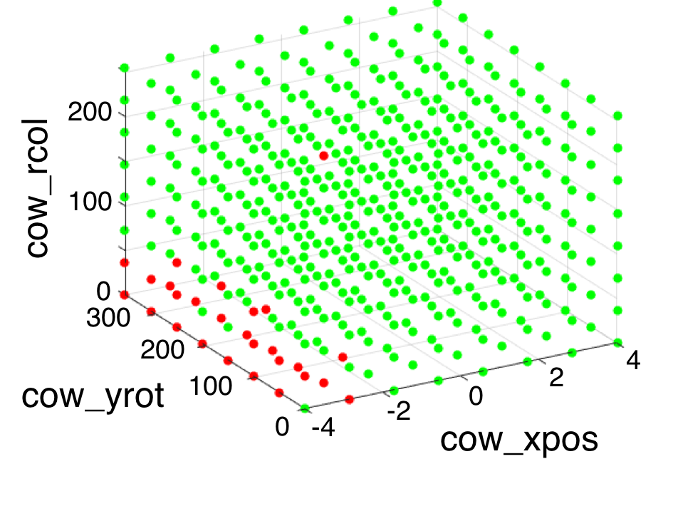
(a) Grid-based sampling.

(b) Halton sequence sampling.

Figure 11: CNN analysis.

Finally, we ran some simulations with the misclassifying images identified by our analysis. Most of them brought the car to collide against the cow. A screenshot of a collision is shown in Figure 9b. The full video is available at https://www.youtube.com/watch?v=MaRoU5OgimE.

6 Conclusion

We presented a compositional falsification framework for STL specifications against CPSML models based on a decomposition between the analysis of machine learning components and the system contained them. We introduced an ML analyzer able to abstract feature spaces, approximate ML classifiers, and provide sets of misclassified feature vectors that can be used to drive the falsification process. We implemented our framework and showed its effectiveness for an autonomous driving controller using perception based on deep neural networks.

This work lays the basis for future advancements. There are several directions for future work, both theoretical and applied. In the remainder of this section, we describe this landscape for future work. See SeshiaS16 for a broader discussion of these points in the context of the goal of verified intelligent systems.

Improvements in the ML Analyzer: We intend to improve our ML Analyzer exploring the automatic generation of feature space abstractions from given training sets. One direction is to exploit the structure of ML components, e.g., the custom architectures that have been developed for deep neural networks in applications such as autonomous driving iandola2016squeezenet . For instance, one could perform a sensitivity analysis that indicates along which axis in the abstract space we should move in order to change the output label or reduce the confidence of the classifier on its output. Another direction is to improve the sampling techniques that we have explored so far, ideally devising one that captures the probability of detecting a corner-case scenario leading to a property violation. Of particular interest are adaptive sampling methods involving further cooperation between the ML Analyzer and the CPS Analyzer. We are also interested in integrating other techniques for generating misclassifications of ML components (e.g., moosavi2015deepfool ; huang-arxiv16 ; carlini-ieeesp17 ) into our approach.

Impacting the ML component design: Our falsification approach produces input sequences that result in the violation of a desired property. While this is useful, it is arguably even more useful to obtain higher-level interpretable insight into where the training data falls short, what new scenarios must be added to the training set, and how the learning algorithms’ parameters must be adjusted to improve accuracy. For example, one could use techniques for mining specifications or requirements (e.g., jin-tcad15 ; vazquez-cav17 ) to aggregate interesting test images or video into a cluster that can be represented in a high-level fashion. One could also apply our ML Analyzer outside the falsification context, such as for controller synthesis.

From Falsification to Verification: The compositional framework we introduced in this paper can also be used for verification of a CPSML model. In particular, if one has a verifier that can prove safety properties of the abstract systems (the optimistic and pessimistic abstractions shown as $\displaystyle M^{-}$ and $\displaystyle M^{+}$ in Figure 2) and one has a systematic refinement strategy that can cover the ROU, then the same compositional framework can be used to prove safety properties of the CPSML model. We plan to explore this direction in future work.

Further Applications: Although our approach has shown initial promise for reasoning about autonomous driving systems, much more remains to be done to make this practical. Real sensor systems for autonomous driving involve multiple sensors (cameras, LIDAR, RADAR, etc.) whose raw outputs are often fused and combined with deep learning or other ML techniques to extract higher level information (such as the location and type of objects around the vehicle). This sensor space has very high dimensionality and high complexity, not to mention streams of sensor input (e.g., video), that one must be able to analyze efficiently. To handle industrial-scale production systems, our overall analysis must be scaled up substantially, potentially via use of cloud computing infrastructure. Finally, our compositional methodology could be extended to other, non-cyber-physical, systems that contain ML components.

References

- [1] Imagenet. http://image-net.org/.
- [2] Udacity self-driving car simulator built with unity. https://github.com/udacity/self-driving-car-sim.
- [3] Y. Annpureddy, C. Liu, G. E. Fainekos, and S. Sankaranarayanan. S-taliro: A tool for temporal logic falsification for hybrid systems. In Tools and Algorithms for the Construction and Analysis of Systems, TACAS, pages 254–257, 2011.
- [4] A. L. Blum and P. Langley. Selection of relevant features and examples in machine learning. Artificial intelligence, 97(1):245–271, 1997.
- [5] M. Bojarski, D. Del Testa, D. Dworakowski, B. Firner, B. Flepp, P. Goyal, L. D. Jackel, M. Monfort, U. Muller, J. Zhang, et al. End to end learning for self-driving cars. arXiv preprint arXiv:1604.07316, 2016.
- [6] M. S. Branicky, S. M. LaValle, K. Olson, and L. Yang. Quasi-randomized path planning. In Robotics and Automation, 2001. Proceedings 2001 ICRA. IEEE International Conference on, volume 2, pages 1481–1487. IEEE, 2001.
- [7] N. Carlini and D. Wagner. Towards evaluating the robustness of neural networks. In Security and Privacy (SP), 2017 IEEE Symposium on, pages 39–57, 2017.
- [8] A. Donzé. Breach, a toolbox for verification and parameter synthesis of hybrid systems. In Computer Aided Verification, CAV, pages 167–170, 2010.
- [9] A. Donzé, T. Ferrere, and O. Maler. Efficient robust monitoring for stl. In Computer Aided Verification, CAV, pages 264–279. Springer, 2013.
- [10] T. Dreossi, T. Dang, A. Donzé, J. Kapinski, X. Jin, and J. Deshmukh. Efficient guiding strategies for testing of temporal properties of hybrid systems. In NASA Formal Methods, NFM, pages 127–142, 2015.
- [11] T. Dreossi, A. Donzé, and S. A. Seshia. Compositional falsification of cyber-physical systems with machine learning components. In NASA Formal Methods Conference (NFM), May 2017.
- [12] T. Dreossi, S. Ghosh, A. L. Sangiovanni-Vincentelli, and S. A. Seshia. Systematic testing of convolutional neural networks for autonomous driving. In ICML Workshop on Reliable Machine Learning in the Wild (RMLW), 2017. Published on Arxiv: abs/1708.03309.
- [13] T. Dreossi, S. Jha, and S. A. Seshia. Semantic adversarial deep learning. In 30th International Conference on Computer Aided Verification (CAV), 2018.
- [14] P. S. Duggirala, S. Mitra, M. Viswanathan, and M. Potok. C2E2: a verification tool for stateflow models. In International Conference on Tools and Algorithms for the Construction and Analysis of Systems, pages 68–82. Springer, 2015.
- [15] A. Fawzi, O. Fawzi, and P. Frossard. Analysis of classifiers’ robustness to adversarial perturbations. arXiv preprint arXiv:1502.02590, 2015.
- [16] B. Hannaford. Resolution-first scanning of multidimensional spaces. CVGIP: Graphical Models and Image Processing, 55(5):359–369, 1993.
- [17] G. Hinton et al. Deep neural networks for acoustic modeling in speech recognition: The shared views of four research groups. IEEE Signal Processing Magazine, 29(6):82–97, 2012.
- [18] X. Huang, M. Kwiatkowska, S. Wang, and M. Wu. Safety verification of deep neural networks. CoRR, abs/1610.06940, 2016.
- [19] F. N. Iandola, S. Han, M. W. Moskewicz, K. Ashraf, W. J. Dally, and K. Keutzer. Squeezenet: Alexnet-level accuracy with 50x fewer parameters and 0.5 mb model size. arXiv preprint arXiv:1602.07360, 2016.
- [20] Y. Jia, E. Shelhamer, J. Donahue, S. Karayev, J. Long, R. Girshick, S. Guadarrama, and T. Darrell. Caffe: Convolutional architecture for fast feature embedding. In ACM Multimedia Conference, ACMMM, pages 675–678, 2014.
- [21] X. Jin, A. Donzé, J. Deshmukh, and S. A. Seshia. Mining requirements from closed-loop control models. IEEE Transactions on Computer-Aided Design of Circuits and Systems, 34(11):1704–1717, 2015.
- [22] A. Krizhevsky, I. Sutskever, and G. E. Hinton. Imagenet classification with deep convolutional neural networks. In Advances in neural information processing systems, pages 1097–1105, 2012.
- [23] O. Maler and D. Nickovic. Monitoring temporal properties of continuous signals. In Formal Techniques, Modelling and Analysis of Timed and Fault-Tolerant Systems, pages 152–166. Springer, 2004.
- [24] Martín Abadi et al. TensorFlow: Large-scale machine learning on heterogeneous systems, 2015. Software available from tensorflow.org.
- [25] J. Matousek. Geometric discrepancy: An illustrated guide, volume 18. Springer Science & Business Media, 2009.
- [26] R. S. Michalski, J. G. Carbonell, and T. M. Mitchell. Machine learning: An artificial intelligence approach. Springer Science & Business Media, 2013.
- [27] S.-M. Moosavi-Dezfooli, A. Fawzi, and P. Frossard. DeepFool: a simple and accurate method to fool deep neural networks. In Proceedings of the IEEE Conference on Computer Vision and Pattern Recognition, pages 2574–2582, 2016.
- [28] W. J. Morokoff and R. E. Caflisch. Quasi-random sequences and their discrepancies. SIAM Journal on Scientific Computing, 15(6):1251–1279, 1994.
- [29] A. Nguyen, J. Yosinski, and J. Clune. Deep neural networks are easily fooled: High confidence predictions for unrecognizable images. In Computer Vision and Pattern Recognition, CVPR, pages 427–436. IEEE, 2015.
- [30] H. Niederreiter. Low-discrepancy and low-dispersion sequences. Journal of number theory, 30(1):51–70, 1988.
- [31] H. Niederreiter. Random number generation and quasi-Monte Carlo methods. SIAM, 1992.
- [32] K. Pei, Y. Cao, J. Yang, and S. Jana. DeepXplore: Automated whitebox testing of deep learning systems. In Proceedings of the 26th Symposium on Operating Systems Principles (SOSP), pages 1–18, 2017.
- [33] J. Rosenblatt and M. Wierdl. Pointwise ergodic theorems via harmonic analysis. In Conference on Ergodic Theory, number 205, pages 3–151, 1995.
- [34] S. A. Seshia, A. Desai, T. Dreossi, D. J. Fremont, S. Ghosh, E. Kim, S. Shivakumar, M. Vazquez-Chanlatte, and X. Yue. Formal specification for deep neural networks. In 16th International Symposium on Automated Technology for Verification and Analysis (ATVA), pages 20–34, 2018.
- [35] S. A. Seshia, D. Sadigh, and S. S. Sastry. Towards verified artificial intelligence. CoRR, abs/1606.08514, 2016.
- [36] P. Shirley et al. Discrepancy as a quality measure for sample distributions. In Proc. Eurographics, volume 91, pages 183–194, 1991.
- [37] I. H. Sloan and S. Joe. Lattice methods for multiple integration. Oxford University Press, 1994.
- [38] C. Szegedy, W. Zaremba, I. Sutskever, J. Bruna, D. Erhan, I. Goodfellow, and R. Fergus. Intriguing properties of neural networks. arXiv:1312.6199, 2013.
- [39] L. Taeyoung, Y. Kyongsu, K. Jangseop, and L. Jaewan. Development and evaluations of advanced emergency braking system algorithm for the commercial vehicle. In Enhanced Safety of Vehicles Conference, ESV, pages 11–0290, 2011.
- [40] Trandafir, Aurel and Weisstein, Eric W. Quasirandom sequence. From MathWorld–A Wolfram Web Resource.
- [41] V. Vapnik. Principles of risk minimization for learning theory. In NIPS, pages 831–838, 1991.
- [42] M. Vazquez-Chanlatte, J. V. Deshmukh, X. Jin, and S. A. Seshia. Logical clustering and learning for time-series data. In Computer Aided Verification - 29th International Conference (CAV), pages 305–325, 2017.
- [43] H. Weyl. Über die gleichverteilung von zahlen mod. eins. Mathematische Annalen, 77(3):313–352, 1916.
- [44] T. Yamaguchi, T. Kaga, A. Donzé, and S. A. Seshia. Combining requirement mining, software model checking, and simulation-based verification for industrial automotive systems. In Proceedings of the IEEE International Conference on Formal Methods in Computer-Aided Design (FMCAD), October 2016.