¹¹institutetext: INAF - Osservatorio Astrofisico di Catania, via S. Sofia, 78, 95123 Catania, Italy ²²institutetext: INAF – Osservatorio Astronomico di Capodimonte, via Moiariello, 16, 80131 Napoli, Italy ³³institutetext: Scientific Support Office, Directorate of Science, European Space Research and Technology Centre (ESA/ESTEC), Keplerlaan 1, 2201 AZ Noordwijk, The Netherlands ⁴⁴institutetext: INAF – Osservatorio Astronomico di Palermo, Piazza del Parlamento 1, I-90134 Palermo, Italy ⁵⁵institutetext: INAF – Osservatorio Astronomico di Roma, via Frascati 33, I-00078 Monte Porzio Catone, Italy

X-Shooter spectroscopy of young stellar objects in Lupus.

Atmospheric parameters, membership and activity diagnostics^†^†thanks: Based on observations collected at the Very Large Telescope of the European Southern Observatory at Paranal, under programs 084.C-0269(A), 085.C-0238(A), 086.C-0173(A), 087.C-0244(A), 089.C-0143(A), 095.C-0134(A), 097.C-0349(A), and archive data of programmes 085.C-0764(A) and 093.C-0506(A). ^,^†^†thanks: Tables 1, 2, and 3 are also available at the CDS via anonymous ftp to cdsarc.u-strasbg.fr (130.79.128.5) or via http://cdsarc.u-strasbg.fr/viz-bin/qcat?J/A+A/?/?.

A. Frasca 11 K. Biazzo 11 J. M. Alcalá 22 C. F. Manara 33 B. Stelzer 44 E. Covino 22 S. Antoniucci 55 antonio.frasca@oact.inaf.it

(Received 22 Nov 2016 / Accepted 3 March 2017)

Abstract

Aims. A homogeneous determination of basic stellar parameters of young stellar object (YSO) candidates is needed to confirm their pre-main sequence evolutionary stage, membership to star forming regions (SFRs), and to get reliable values of the quantities related to chromospheric activity and accretion.

Methods. We used the code ROTFIT and synthetic BT-Settl spectra for the determination of the atmospheric parameters ( $T_{\rm eff}$ and $\log g$ ), the veiling ( $r$ ), the radial (RV) and projected rotational velocity ( $v\sin i$ ), from X-Shooter spectra of 102 YSO candidates (95 of infrared Class II and seven Class III) in the Lupus SFR. The spectral subtraction of inactive templates, rotationally broadened to match the $v\sin i$ of the targets, enabled us to measure the line fluxes for several diagnostics of both chromospheric activity and accretion, such as H $\alpha$ , H $\beta$ , Ca ii and Na i lines.

Results. We have shown that 13 candidates can be rejected as Lupus members based on their discrepant RV with respect to Lupus and/or the very low $\log g$ values. At least 11 of them are background giants, two of which turned out to be lithium-rich giants. Regarding the members, we found that all Class III sources have H $\alpha$ fluxes compatible with a pure chromospheric activity, while objects with disks lie mostly above the boundary between chromospheres and accretion. YSOs with transitional disks displays both high and low H $\alpha$ fluxes. We found that the line fluxes per unit surface are tightly correlated with the accretion luminosity ( $L_{\rm acc}$ ) derived from the Balmer continuum excess. This rules out that the relationships between $L_{\rm acc}$ and line luminosities found in previous works are simply due to calibration effects. We also found that the Ca ii-IRT flux ratio, $F_{\rm CaII8542}/F_{\rm CaII8498}$ , is always small, indicating an optically thick emission source. The latter can be identified with the accretion shock near the stellar photosphere. The Balmer decrement reaches instead, for several accretors, high values typical of optically thin emission, suggesting that the Balmer emission originates in different parts of the accretion funnels with a smaller optical depth.

Key Words.:

stars: pre-main sequence, fundamental parameters, chromospheres – accretion – open clusters and associations: Lupus

^†^†offprints: A. Frasca

1 Introduction

A full characterization of members of young open clusters (OCs) and star forming regions (SFRs) is necessary to understand the mechanisms of star and planet formation, as well as the different phenomena occurring during the early phases of stellar evolution. It is therefore mandatory to derive, as homogeneously as possible, the basic physical parameters of young stellar objects (YSOs), such as effective temperature ( $T_{\rm eff}$ ), surface gravity ( $\log g$ ), mass and projected rotational velocity ( $v\sin i$ ). These quantities are closely related to the evolutionary stage of the YSO and are also directly involved in the generation of stellar magnetic fields by the dynamo processes. In the context of the magnetospheric accretion model, magnetic fields play a key role in the infall of matter from the disk onto the central star (Hartmann et al. 1994, 2016, and references therein). They are also responsible for the strong activity observed from the photospheres to the chromospheres and coronae of YSOs and late-type stars in general (e.g., Feigelson & Montmerle 1999; Berdyugina 2009, and references therein). Circumstellar disks, stellar rotation, magnetic activity and accretion are all strongly involved in the process of planet formation (e.g., Hawley & Balbus 1991; Brandenburg et al. 1995; Larson 2003, and references therein).

Deriving the basic stellar parameters is particularly hard for objects belonging to very young OCs and SFRs where several phenomena, such as fast rotation, cloud extinction and mass accretion, affect their spectra, making the analysis of their photospheres difficult. In particular, the veiling of the spectra, arising from accretion shocks and, possibly, from disk gas inside the dust sublimation radius, dilutes the photospheric lines and it must be properly taken into account to derive reliable stellar parameters (see, e.g., Frasca et al. 2015, and references therein). Moreover, emission lines, which are numerous and very strong and broad in the spectra of highly accreting objects, need to be masked, leaving only limited spectral ranges suitable for the analysis of photospheric lines.

On the other hand, it is well known that the luminosity of several emission lines of the Balmer series, the He i and Ca ii lines are well correlated with the accretion luminosity (e.g., Herczeg & Hillenbrand 2008; Alcalá et al. 2014, 2017, and references therein), as well as with hydrogen recombination lines in the near-infrared (Muzerolle et al. 1998; Calvet et al. 2004; Alcalá et al. 2017), highlighting the importance of these emission features as accretion diagnostics.

Spectra with both a very wide wavelength coverage and a high or intermediate resolution are particularly helpful, as they offer the possibility to find spectral intervals free from or little affected by these issues, where fully resolved absorption lines can be modeled to consistently derive atmospheric parameters, radial velocity, $v\sin i$ , and veiling. For this reason, the VLT/X-Shooter spectrograph (Vernet et al. 2011), with its wide wavelength coverage, is an ideal instrument to reach these goals.

Thanks to their relatively close distance to the Sun (150–200 pc, Comerón 2008) and the large numbers of Class II and Class III infrared sources they contain, the dark clouds in Lupus are among the best sites for which a spectroscopic determination of the atmospheric parameters for YSOs can be carried out down to the hydrogen burning mass limit. In addition, extinction to the individual YSOs is relatively low in comparison with many other SFRs.

The selection of candidates and the characterization of some of the confirmed Lupus members, both physical and kinematical, has been performed in recent years (see, e.g., Evans et al. 2009; Comerón et al. 2009, 2013; Galli et al. 2013; Herczeg & Hillenbrand 2014; Bustamante et al. 2015). However, most of these works are based on non-simultaneous optical and IR photometry and low-resolution spectroscopy. Moreover, the atmospheric parameters are derived mostly for the Class III sources. A homogeneous determination of the atmospheric parameters, $v\sin i$ , and veiling for a large sample of Class II sources in Lupus is still lacking. In this work we aimed at filling-in this gap. Our study is based on X-Shooter spectra of more than one hundred YSO candidates in the Lupus I, II, III, and IV clouds.

The high quality and the intermediate resolution of these spectra allowed us also to investigate the behavior of hydrogen, calcium and sodium emission lines that are diagnostics of both chromospheric and accretion activity.

The paper is organized as follows. In Sect. 2 we present the data sample. The analysis of the spectra for the determination of stellar parameters and the radial velocities is described in Sect. 3. The results are discussed in Sect. 4, where the properties of the targets, the membership to the Lupus SFR, and the line fluxes per unit surface are discussed. The main conclusions are summarized in Sect. 5.

2 Data sample

In total, we analyzed X-Shooter spectra of 102 objects, 43 of which were obtained in 2010, 2011, and 2012, during the INAF guaranteed time observations (GTO, Alcalá et al. 2011a). The remaining sources were observed in the framework of the ESO-P95 proposal from March to August 2015 (48 objects) and the ESO-P97 proposal from May to June 2016 (5 objects). In addition, X-Shooter spectra of six YSOs were retrieved from the ESO archive. Our sample comprises sources belonging to the infrared (IR) Class II. However, seven Class III objects were also included. Six of them have been already investigated by Stelzer et al. (2013) and Manara et al. (2013). The sample accounts for roughly half of the entire known population of YSOs in Lupus, but $\sim$ 95 % of disky YSOs. For the criteria of target selection and details about the data reduction the reader is referred to Alcalá et al. (2014, 2017).

We remark that 13 out of the 103 objects studied here were suspected to be non-members based on the appearance of their spectrum (Alcalá et al. 2017). The analysis we performed in this work allowed us to definitely reject them as members.

The target list is given in Table 1 together with the heliocentric Julian Date of observation and some of the parameters derived in this work. The spectra of Sz 68, Sz 74, Sz 83, Sz 102, Sz 105, and the archive data (i.e., IM Lup, Sz 77, EX Lup, GQ Lup, Sz 76, RXJ1556.1-3655) were acquired using the 0 $\aas@@fstack{\prime\prime}$ 5/0 $\aas@@fstack{\prime\prime}$ 4/0 $\aas@@fstack{\prime\prime}$ 4 slits in the UVB/VIS/NIR arms, respectively. All the other targets were instead observed with the 1 $\aas@@fstack{\prime\prime}$ 0/0 $\aas@@fstack{\prime\prime}$ 9/0 $\aas@@fstack{\prime\prime}$ 9 slits in the UVB/VIS/NIR arms, respectively.

For our analysis, particularly for the $v\sin i$ measurement, it is important to know the actual spectral resolution. To this purpose we used Th-Ar calibration spectra taken during our observing runs. We found that the resolving power of VIS spectra taken with the 0 $\aas@@fstack{\prime\prime}$ 9 slit was $R\simeq 8400$ in the spectral region used for the $v\sin i$ determination ( $\lambda\sim$ 9700Å), while in the highest resolution mode (0 $\aas@@fstack{\prime\prime}$ 4 slit) it is about 17 000. More details can be found in Appendix A.

3 Atmospheric parameters, veiling, radial and projected rotational velocities

The determination of the atmospheric parameters ( $T_{\rm eff}$ and $\log g$ ), the veiling $r$ , the projected rotational velocity ( $v\sin i$ ) and the radial velocity (RV) was accomplished through the code ROTFIT (e.g., Frasca et al. 2006, 2015).

We adopted as templates a grid of synthetic BT-Settl spectra (Allard et al. 2012) with a solar iron abundance and effective temperature in the range 2000–6000 K (in steps of 100 K) and $\log g$ from 5.5 to 0.5 dex (in steps of 0.5 dex). This grid covers the wide range in spectral type (SpT), from early-K to late-M, spanned by our targets and extends also to lower gravities typical of giants.

The code ROTFIT was already applied to X-Shooter spectra of Class III sources in Stelzer et al. (2013). However, the code was improved since then with the inclusion of further spectral segments to be analyzed both in the VIS and UVB spectra. Furthermore, in this version we implemented an accurate search for the minimum of the chi-square ( $\chi^{2}$ ) in the space of parameters and the evaluation of the errors based on the 1 $\sigma$ confidence levels. The veiling, $r$ , was also considered as a free parameter. Details on the application of the code to the X-Shooter spectra are given in Appendix B.

3.1 Radial velocity

The RV was needed to align the synthetic template spectra with the observed ones. The peak of the cross-correlation function (CCF) was fitted with a Gaussian for a more accurate determination of its center (see the insets in Fig. 19). For each i^th spectral segment, the error of the $RV_{\rm i}$ value, $\sigma_{RV_{\rm i}}$ , was estimated by the fitting procedure curvefit (Bevington 1969), taking into account the CCF noise, which was evaluated as the standard deviation of the CCF values outside the peak. Then, the heliocentric correction of the RV measurements was performed with the IDL procedure helcorr. The final RV for each star, reported in Table 1, is the weighted mean of the values obtained from all analyzed spectral segments, using as weights $w_{\rm i}=1/\sigma_{RV_{\rm i}}^{2}$ . The standard error of the weighted mean was adopted as the RV uncertainty. These errors range from 0.7 to 12 km s^-1, with a median value of 2.3 km s^-1. We note that, as expected, the RV errors tend to be larger for the stars with higher $v\sin i$ and/or with low S/N spectra, or strongly affected by veiling (see Table 1).

3.2 Accuracy of $T_{\rm eff}$ and $\log g$ determinations and comparisons with the literature

The $T_{\rm eff}$ errors reported in Table 1 range from about 30 to 250 K, depending on $T_{\rm eff}$ (and on the S/N), with a median value of 70 K. The only exception is SSTc2dJ161045.4-385455 ( $\sigma_{T_{\rm eff}}$ = 514 K), a likely non-member with a low-signal spectrum.

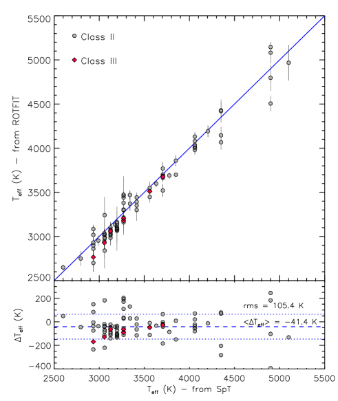
Refer to caption — Figure 1: Top panel) Comparison between the effective temperature determined with ROTFIT and that derived from the MK spectral classification performed for the Lupus members by Manara et al. (2013) and Alcalá et al. (2014, 2017). The continuous line in the top panel represents the 1:1 relationship. The $T_{\rm eff}$ differences (Bottom panel) show a mean value of about $-40$ K (dashed line) and a standard deviation of about 100 K (dotted lines).

To estimate the external accuracy of $T_{\rm eff}$ , we have compared our values with those derived from the spectral classification performed by Manara et al. (2013) for the Class III objects and by Alcalá et al. (2014, 2017) for the Class II sources, who adopted the temperature scales of Luhman et al. (2003) and Kenyon & Hartmannn (1995) for the M- and K-type stars, respectively. The comparison is shown in Fig. 1. The general agreement of the two $T_{\rm eff}$ determinations is evident, with a scatter of the residuals $\simeq$ 100 K rms. Nevertheless, this comparison displays a systematic offset between the two $T_{\rm eff}$ determinations, which is more evident in the M-type domain, with the $T_{\rm eff}$ values derived from SpT being about 40 K higher, on average, than those from ROTFIT. This offset is likely due to the different $T_{\rm eff}$ scales between the BT-Settl models and the empirical SpT– $T_{\rm eff}$ calibration defined for M-type stars by Luhman et al. (2003). We note that the $T_{\rm eff}$ values of Luhman et al. (2003) for early M-type stars are systematically higher by $\sim$ 70 K than those reported by Pecaut & Mamajek (2013) for young stars, which are based on the fitting of the optical/IR spectral energy distributions.

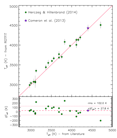
As a further check for the accuracy of our determinations we have searched for spectroscopic $T_{\rm eff}$ measurements in the literature, not based on X-Shooter data. We compared our results with the values reported by Comerón et al. (2013) and Herczeg & Hillenbrand (2014). Both works are based on low resolution ( $R=500$ –1000) optical spectra. We have only one star in common with Comerón et al. (2013), namely SSTc2d160836.2-392302, for which the $T_{\rm eff}$ agreement is excellent (see Fig. 2). Twenty of our targets have been observed by Herczeg & Hillenbrand (2014), who list the spectral type derived from suitable spectral indices. We converted their SpT into $T_{\rm eff}$ by using the calibration put forward by them. The comparison is displayed in Fig. 2. The agreement is evident, with an average offset of +28 K and a scatter of about 100 K, as in Fig. 1. The latter can be considered as the typical external accuracy of our $T_{\rm eff}$ values. We note that, despite the lower number of points, the agreement in the M-type domain looks better than the one shown in Fig. 1. This is likely owing to the $T_{\rm eff}$ scale, based on BT-Settl spectra, adopted both in the present work and in Herczeg & Hillenbrand (2014).

Concerning $\log g$ , the errors are in the range 0.1–0.5 dex, with a median value of 0.21 dex. Only four objects have larger errors (up to 0.9 dex). We did not find other estimates of gravity in the literature, except for the value of $\log g$ =4.0 reported by Comerón et al. (2013) for SSTc2d160836.2-392302, which is consistent with ours (4.04 $\pm$ 0.13).

3.3 Projected rotational velocity

The intermediate resolution of X-Shooter allows us to measure $v\sin i$ only for relatively fast rotators. To check the minimum $v\sin i$ that can be measured in these spectra and to estimate the $v\sin i$ errors, we have run Monte Carlo simulations on synthetic spectra with the same resolution and sampling of X-Shooter, following the prescriptions given in Frasca et al. (2015). We found that the minimum detectable $v\sin i$ with the 0 $\aas@@fstack{\prime\prime}$ 9 slit is about 8 km s^-1. Therefore, we considered as upper limits all $v\sin i$ values lower than 8 km s^-1. We also evaluated the upper limit on $v\sin i$ for the spectra acquired with the 0 $\aas@@fstack{\prime\prime}$ 4 slit, finding a value of 6 km s^-1. Details about the Monte Carlo simulations can be found in Appendix C. The errors of $v\sin i$ range from 1 to 15 km s^-1(Table 1), with a median value of about 4 km s^-1.

Determinations of $v\sin i$ can be found in the literature only for a handful of the brightest sources in our sample. For Sz 68, Torres et al. (2006) report a value of $v\sin i$ $=38.9\pm 0.6$ km s^-1, which is compatible with our determination of 39.6 $\pm 1.2$ km s^-1. Dubath et al. (1996) give only a lower limit of $v\sin i$ $>60$ km s^-1 for Sz 121, which is one of the most rapidly rotating stars in our sample ( $v\sin i$ $=87$ km s^-1). The same authors report $v\sin i$ $=10.2\pm 1.6$ km s^-1 for Sz 108, for which we find an upper limit of 8 km s^-1. The value of 22.4 km s^-1 quoted in the Catalog of Stellar Rotational Velocities (Glebocki & Gnacinski 2005) for RY Lup is marginally consistent with ours ( $v\sin i$ $=16.3\pm 5.3$ km s^-1). Finally, in the same catalog, $v\sin i$ $=14.2$ km s^-1 is reported for Sz 98, while we find $v\sin i$ $<8$ km s^-1.

3.4 Veiling

After several tests made with our code on Class III and X-Shooter archive spectra of non-accreting stars, we realized that values of veiling as large as 0.2 can be found, although no veiling is expected in such cases. This is probably a combined effect of the intermediate spectral resolution, small differences in the continuum setting between target and template spectra, and some trade-off between parameters. For this reason, all values $r\leq 0.2$ are considered as not significant and have been replaced with an upper limit of 0.2 in Table 1. We measured significant values of veiling ( $r>0.2$ ) for 12, 19, and 44 YSOs at 970 nm, 710 nm, and 620 nm, respectively. This trend is in line with the enhancement of $r$ with decreasing wavelength (see Fig. 22).

Herczeg & Hillenbrand (2014) report values of the veiling at 750 nm for sixteen of our targets. For about a half of them we derived only upper limits, $r_{710}\leq 0.2$ , while for the remaining YSOs the veiling is always rather small. However, the comparison of these data shows that we can measure the veiling at 710 nm whenever Herczeg & Hillenbrand (2014) quote $r_{750}>0.2$ .

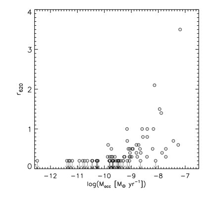
Using the mass accretion rates derived by Alcalá et al. (2017) on the same data set, we found that high values of veiling ( $r_{620}\geq 1.0$ ) are measured only for the strongest accretors ( $\dot{M}_{\rm acc}$ $>10^{-9}$ , see Fig. 3).

4 Results

4.1 Membership

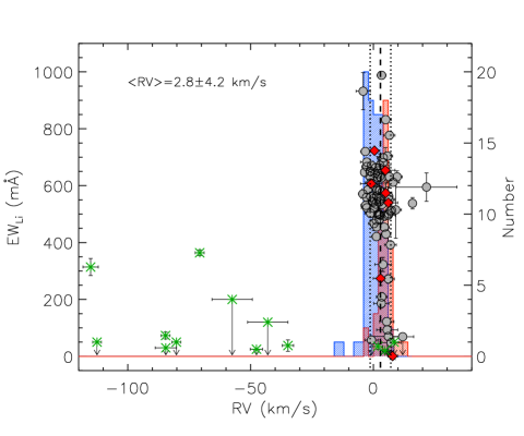
The atmospheric parameters, the RV, and the equivalent width of the lithium line at 6707.8 Å ( $EW_{\rm Li}$ ) were used to verify the membership of our targets to the Lupus SFR. Here we used the $EW_{\rm Li}$ values derived by Biazzo et al. (2016).

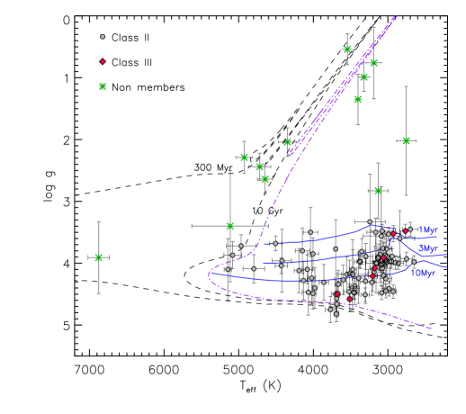
The $\log g$ values derived with ROTFIT allow us to identify in our sample contaminants whose IR colors mimic those of cool very young stars. In Fig. 4 we show the $\log g$ - $T_{\rm eff}$ diagram of our targets, where the stars suspected to be non-members have been highlighted with green asterisks. We also plot the pre-main sequence (PMS) isochrones of Baraffe et al. (2015) and the post-main sequence isochrones from the PARSEC database (Bressan et al. 2012).

All green asterisks at $T_{\rm eff}$ $<5000$ K have $\log g<3.0$ and correspond most likely to giants. Four of these are indeed in the red giant branch (RGB) and possibly close to the red giant clump; a few others, with lower gravity, could be in the AGB phase. The star with the highest temperature, SSTc2dJ161148.7-381758, could be a MS star unrelated to the Lupus SFR, as indicated by its RV= $-47.6$ km s^-1. The green asterisk with the largest errors located at $T_{\rm eff}$ =5114 K and $\log g$ =3.4 corresponds to SSTc2dJ161045.4-385455. Its position on the $\log g$ - $T_{\rm eff}$ plane may be compatible with the PMS locus, taking into account the errors, but the value of RV= $-115.1$ km s^-1 strongly suggests that it is not a member of the Lupus SFR.

The other two indicators of membership, namely the RV and $EW_{\rm Li}$ , are plotted in Fig. 5 with the same symbols as in Fig. 4. It is worth noting that, except for two objects (SSTc2dJ160708.6-394723 and SSTc2dJ161045.4-385455), all the stars classified as non-members based on the $\log g$ - $T_{\rm eff}$ diagram and/or discrepant RV, have undetectable Li i lines. The non-member with the highest $EW_{\rm Li}$ (364 mÅ) is SSTc2dJ160708.6-394723. For this object we estimate $T_{\rm eff}$ $\simeq\,4650$ K and $\log g$ $\simeq 2.6$ , thus it lies in the RGB region of the $\log g$ - $T_{\rm eff}$ diagram (Fig. 4). Its RV is inconsistent with the Lupus SFR. Likewise, SSTc2dJ161045.4-385455 has a rather large $EW_{\rm Li}$ (about 300 mÅ), but, as already mentioned, its RV = $-115.1$ km s^-1 and the absence of emission lines rule out its membership to the Lupus SFR. Although with large errors, its atmospheric parameters suggest a G-type giant or subgiant. These two stars are most likely lithium-rich giants. More details are given in Appendix D.

Three other non-members based on the $\log g$ - $T_{\rm eff}$ diagram (Sz 78, Sz 105, and SSTc2dJ161222.7-371328) have instead RVs compatible with Lupus, but no Lithium. These stars have all very low $\log g$ values of 2.04, 0.76, and 0.99, respectively, thus ruling out a PMS nature.

In conclusion, by using the three indicators, $\log g$ , RV, and $EW_{\rm Li}$ , we were able to reject 13 stars as Lupus members. All the remaining 89 targets were considered as members, although a few of them have an RV slightly outside the SFR average derived by us ( $<RV>=2.8\pm 4.2$ km s^-1) and external to the RV distributions for on-cloud and off-cloud sources defined by Galli et al. (2013). Nonetheless, they display a large $EW_{\rm Li}$ that reinforces their membership; they could be spectroscopic binaries.

A small group of six Class II sources, namely Sz 69, Lup706, Par-Lup3-4, 2MASS J16085953-3856275, 2MASS J16085373-3914367, and SSTc2dJ154508.9-341734, has instead an RV well consistent with the Lupus SFR but a quite low lithium content ( $EW_{\rm Li}<150$ mÅ). Nevertheless, the spectra of these objects display other features that indicate their membership (c.f. strong and wide emission lines, veiling, etc., Alcalá et al. 2014, 2017). These cases will be discussed in more detail in Biazzo et al. (2016). Finally, the star Sz 94, classified as a Class III source with proper motions and RV compatible with Lupus, shows $EW_{\rm Li}\approx 0$ , making its membership dubious.

4.2 Hertzsprung-Russell diagram

In Alcalá et al. (2017) we derived masses using four different evolutionary tracks, but only for the Class II sources. Here we derive masses and ages for both the Class III and Class II sources homogeneously, and using the $T_{\rm eff}$ values resulting from the ROTFIT analysis.

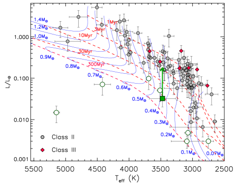
In Fig. 6, we report the position of our targets in the Hertzsprung-Russell (HR) diagram, where we used the $T_{\rm eff}$ values derived in the present work and the luminosities calculated by Manara et al. (2013) and Alcalá et al. (2014, 2017), with the same method, for the Class III and Class II sources, respectively. In the same figure we overplot the PMS evolutionary tracks and isochrones by Baraffe et al. (2015).

Most of the targets are located between the isochrones at 1 and 10 Myr, while a few of them (Lup706, Sz106, Par-Lup3-4, Sz123B, Sz133, SSTc2dJ160703.9-391112, and Sz102), displayed with larger open circles in Fig. 6, appear to be subluminous. These are likely objects with rotation axes perpendicular to the line of sight where the edge-on disks reduce the stellar luminosity by extinction and light scattering (Alcalá et al. 2014, 2017). Several of these objects show in their optical spectra an enhancement of outflow tracers like the low-velocity component of the O i $\lambda$ 6300 Å line (Bacciotti et al. 2011; Natta et al. 2014; Whelan et al. 2014). This line originates in a more extended volume with respect to the accretion tracers that arise from a much closer region to the stellar surface, and are suppressed by the optically thick edge-on disk. This effect is particularly important in Par-Lup3-4, Sz102 and Sz133 (Bacciotti et al. 2011, Natta et al. 2014, Nisini et al. in prep.). Another object, namely SSTc2dJ160708.6-391408, classified as a flat IR source (Merín et al. 2008) and shown with a green filled square in Fig. 6, appears subluminous because the derived stellar luminosity does not account for reprocessed stellar radiation in the infalling envelope of gas and dust (see Appendix C in Alcalá et al. 2017). This object is further discussed in Appendix D.

The evolutionary tracks and isochrones can be used to estimate the masses and ages of the targets from their location in the HR diagram by minimizing the quantity:

\chi^{2}=\frac{(T_{\rm eff}-T_{\rm mod})^{2}}{\sigma_{T_{\rm eff}}^{2}}+\frac{(L-L_{\rm mod})^{2}}{\sigma_{L}^{2}}\,,

(1)

where $T_{\rm eff}$ and $L$ are the stellar effective temperature and bolometric luminosity, respectively, with errors $\sigma_{T_{\rm eff}}$ and $\sigma_{L}$ , respectively. The effective temperature and stellar luminosity of the evolutionary tracks are denoted with $T_{\rm mod}$ and $L_{\rm mod}$ , respectively. We assigned to each YSO the mass and age corresponding to the closest track and isochrone, which minimize $\chi^{2}$ .

The same procedure was used for evaluating masses and ages with the Siess et al. (2000) evolutionary models that do not cover the very low-mass regime but extend to higher masses. For the stars in the mass range 0.1–1.4 $M_{\sun}$ we found an excellent agreement between the masses derived with the two sets of tracks, with differences within 0.05 $M_{\sun}$ rms. Masses and ages, with the exception of the underluminous sources, are reported in Table 1. For the most massive star, SSTc2dJ160830.7-382827, whose position in the HR diagram is outside the mass range covered by the Baraffe et al. (2015) tracks, we adopted the Siess et al. (2000) models and we found $M_{\star}$ =1.8 $M_{\odot}$ and $Age=2.9$ Myr.

The mass determinations are in very close agreement with those of Alcalá et al. (2017). As stressed in previous works, the age determination suffers from uncertainties due to the error on the distance of the clouds, source variability, extinction and depends on the adopted set of evolutionary tracks (see, e.g., Comerón 2008, and references therein). Therefore, the ages of the individual sources are affected by large uncertainties. However, the median age of the full sample analyzed in the present work is 2 Myr and the average value is 2.5 Myr, in good agreement with previous determinations (e.g., Alcalá et al. 2014, 2017, and references therein).

4.3 Activity/accretion diagnostics

The emission lines comprised in the X-Shooter spectra have been used as diagnostics of chromospheric activity and accretion in previous works of our group (e.g., Stelzer et al. 2013; Alcalá et al. 2014). We have shown how the exceptional richness of information of these spectra allows us to probe the different layers of the atmospheres of PMS stars and to define the “noise” that chromospheric emission introduces into mass accretion estimates (Manara et al. 2013). These spectra allowed us to considerably improve the accuracy of the determination of mass accretion with important implications on the $\dot{M}_{\rm acc}$ – $M_{\star}$ relationship (Alcalá et al. 2014, 2017).

Here we give a closer look at the H $\alpha$ , Ca ii K, Ca ii infrared triplet (IRT), and Na i D_1,2. These lines, particularly H $\alpha$ and Ca ii lines, have been widely used as diagnostics for both chromospheric activity (e.g., Strassmeier et al. 2000; Montes et al. 2001; Martínez-Arnáiz et al. 2011; Frasca et al. 2016, and reference therein) and accretion (e.g., Muzerolle et al. 2003; Mohanty et al. 2005; Costigan et al. 2012; Alcalá et al. 2014) due to their intensity and the high sensitivity of the CCD detectors at these wavelengths. The cores of the Na i D_1,2 lines are good diagnostics of chromospheric activity (especially in late-K and M-type stars, e.g., Houdebine et al. 2009; Gomes da Silva et al. 2011), mass accretion (e.g., Rigliaco et al. 2012; Alcalá et al. 2014, 2017) and winds (e.g., Natta & Giovanardi 1990; Facchini et al. 2016).

We calculated the equivalent widths (EWs) and line fluxes by using the spectral subtraction method (see, e.g., Frasca & Catalano 1994; Montes et al. 1995) to remove the photospheric flux and to evidence the core emission. Although this correction is negligible for objects with high accretion rates and very strong emission lines, it is absolutely needed in cases where the photospheric profile is only filled-in with emission or the latter is very weak.

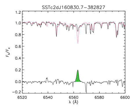
Figure 7 shows the result of the spectral subtraction on the H $\alpha$ line of SSTc2dJ160830.7-382827, which is a target with a transitional disk and a weak accretor (Alcalá et al. 2017). In this case the H $\alpha$ line displays an absorption profile filled-in with emission, which is only revealed by subtracting the inactive template. The latter has been obtained by the interpolation of the best-fitting BT-Settl spectra at the $T_{\rm eff}$ and $\log g$ of the target that are quoted in Table 1.

The inactive templates are rotationally broadened, whenever $v\sin i$ is larger than the minimum value that can be resolved by the observations (see Sect. 3.3), Doppler-shifted, and resampled on the spectral points of the target spectra before subtraction. The residual H $\alpha$ profile integrated over wavelength (hatched green area in Fig. 7) provides us with the net H $\alpha$ EW.

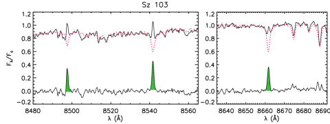
An example of the application of the spectral subtraction method to the Ca ii IRT lines is shown in Fig. 8 for the star Sz 103. We note that the subtraction of the inactive template is necessary for a correct measurement of the Ca ii IRT EWs. In particular, the Ca ii $\lambda$ 8662 line shows an emission in its core that does not reach the continuum.

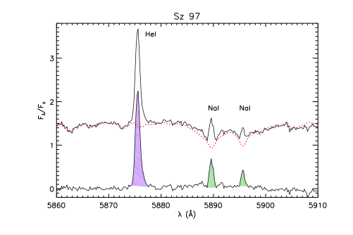
The result of the spectral subtraction in the region of Na i D_1,2 and He i D₃ lines for Sz 97 is shown in Fig. 9. It is clear that, although the underlying photospheric spectrum barely affects the strong He i D₃ line, it must be subtracted from the target spectrum to get the emission EWs in the Na i D_1,2 line cores. We stress that the X-Shooter spectra were corrected for telluric absorption lines also at these wavelengths, as described by Alcalá et al. (2014), and the interstellar Na i absorption affects significantly only the more distant non-members (giants).

We converted the observed EWs into line fluxes per unit surface by multiplying them for the continuum flux of the synthetic spectrum corresponding to the $T_{\rm eff}$ and $\log g$ of the target. To get a more accurate value of the continuum flux, we interpolated in $T_{\rm eff}$ and $\log g$ within the grid of BT-Settl spectra. The fluxes of H $\alpha$ , H $\beta$ , Ca ii K, Ca ii IRT, and Na i D lines are quoted in Table 2. In this table we do not report any flux value whenever the spectral subtraction does not give an emission residual profile. We treat as upper limits the values for which the error is larger than the flux.

We have already shown in Stelzer et al. (2013) the agreement between line fluxes per unit surface calculated on the basis of model spectra, as in the present paper, and those derived from the observed flux at Earth and the dilution factor, $(R_{*}/d)^{2}$ , where $R_{*}$ and $d$ are the stellar radius and distance, respectively.

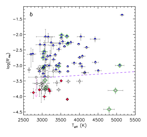
We also calculated the ratio of the line and bolometric flux, $R^{\prime}_{\rm line}=F_{\rm line}/(\sigma T_{\rm eff}^{4})$ as a further chromospheric/accretion diagnostic¹¹1The prime in $R^{\prime}_{\rm line}$ indicates that the photospheric contribution was subtracted, as usual in the definition of activity indices..

For the stars with H $\alpha$ line in emission above the local continuum, we also measured the full width at 10% of the line peak ( $10\%W_{\rm H\alpha}$ ). This quantity is helpful for discriminating between accreting stars and those with pure chromospheric emission. In particular, we defined “candidate accretors” the objects that fulfill the criterion of White & Basri (2003) that is based on both a $10\%W_{\rm H\alpha}\geq 270$ km s^-1 and $EW_{H\alpha}$ larger than given thresholds depending on spectral type, and distinguished them in the following plots with half-filled symbols.

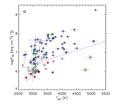
In Fig. 10 we plot the H $\alpha$ flux, $F_{\rm H\alpha}$ , and the ratio $R^{\prime}_{\rm H\alpha}$ as a function of the effective temperature. In this figure, the boundary between the accreting objects and the chromospherically active stars, as defined by Frasca et al. (2015) with the same criteria for the members of the Gamma Vel cluster and Cha I SFR, is also marked. We note that all Class III stars lie below the aforementioned boundary and all “candidate accretors” (half-filled symbols) are located above it, while the other Class II sources are scattered around, and mostly below, this dividing line. In particular, 17 Class II sources are located below the dividing line. However, this border cannot be considered as a knife edge that separates accretors from chromospheric sources; therefore only the objects lying well below it are noteworthy. For instance, if we select only the YSOs with $\log(R^{\prime}_{\rm H\alpha})\leq-3.7$ , where most of the Class III sources lie, we end up with only eight Class II sources, three of which (Lup 607, MY Lup, and SSTc2dJ160830.7-382827) are those considered as “weak accretors” by Alcalá et al. (2017). The other five objects, namely SSTc2dJ160000.6-422158, SSTc2dJ155925.2-423507, Sz 95, SSTc2dJ161029.6-392215, and SSTc2dJ160703.9-391112 have rather low accretion rates according to Alcalá et al. (2017). The low H $\alpha$ flux could indicate that these objects have still rather dense dusty disks that give rise to the IR excess, but a low or moderate accretion rate for which the H $\alpha$ flux is comparable with that of chromospheric sources.

The presence above the dividing line of some Class II object with a substantial accretion rate (Alcalá et al. 2017) and not satisfying the White & Basri criterion shows that the latter is not 100 % reliable in selecting accretors.

We note that the objects with transitional disks (TD), shown as green open diamonds in Fig. 10, are spread all over the diagram and no clear behavior appears, in agreement with the finding by Alcalá et al. (2017) for the mass accretion rate.

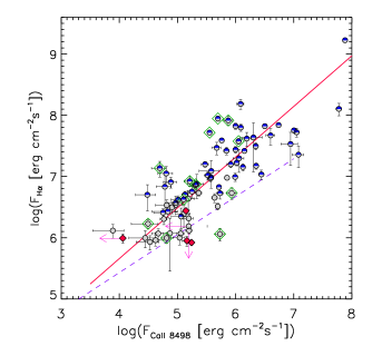
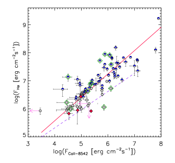
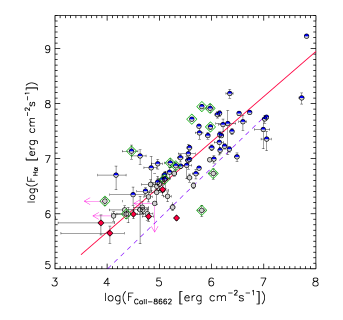
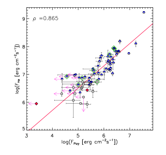
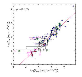
The H $\alpha$ and Ca ii IRT fluxes are well correlated, as apparent in Fig. 11 and suggested by the high value of Spearman’s rank correlation coefficients, which range from $\rho=0.80$ to $\rho=0.83$ with a significance $\sigma$ in the range $10^{-22}$ – $10^{-19}$ (Press et al. 1992), for the three Ca ii lines. Least-squares regressions provide the following relations:

$\displaystyle\log F_{\rm H\alpha}$	$\displaystyle=$	$\displaystyle 2.35(\pm 0.32)+0.83(\pm 0.07)\cdot\log F_{\rm CaII8498}$
$\displaystyle\log F_{\rm H\alpha}$	$\displaystyle=$	$\displaystyle 2.23(\pm 0.29)+0.84(\pm 0.06)\cdot\log F_{\rm CaII8542}$
$\displaystyle\log F_{\rm H\alpha}$	$\displaystyle=$	$\displaystyle 2.38(\pm 0.27)+0.82(\pm 0.07)\cdot\log F_{\rm CaII8662}.$	(2)

It is worth noting that most of the sources display H $\alpha$ fluxes in excess with respect to the mean flux-flux relations found by Stelzer et al. (2013) for Class III objects in Lupus, TWA, and $\sigma$ Ori SFRs. This is particularly evident for the “candidate accretors” (half-filled symbols) and suggests that the accretion produces a larger H $\alpha$ luminosity, compared to Ca ii IRT lines, than that originating from chromospheres. This trend can be explained by the fact that strong accretors generally have also outflows or stronger winds, which contribute to the H $\alpha$ emission but do not significantly affect Ca ii lines.

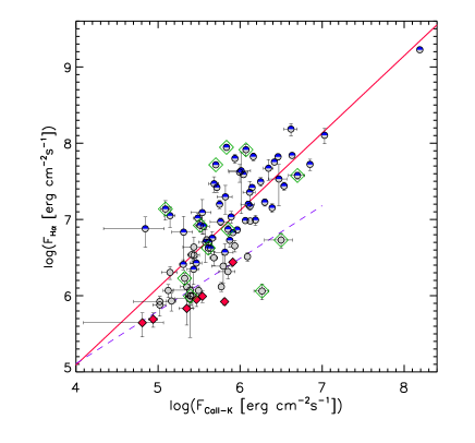
A similar behavior is found when plotting the H $\alpha$ versus the Ca ii K flux, as displayed in Fig. 12. These data can be fitted by the following linear relation:

\displaystyle\log F_{\rm H\alpha}

\displaystyle=

\displaystyle 1.04(\pm 0.41)+1.01(\pm 0.07)\cdot\log F_{\rm CaIIK}

(3)

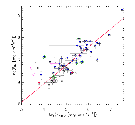
The H $\alpha$ and Na i D_1,2 fluxes display a correlation ( $\rho=0.81$ , $\sigma=7\cdot 10^{-15}$ ), as shown in Fig. 13. We remark that $F_{\rm NaID}$ is the sum of the fluxes in the two sodium D lines. A least-squares regression provides the following relation:

\log F_{\rm H\alpha}=2.67(\pm 0.38)+0.82(\pm 0.09)\cdot\log F_{\rm NaID}.

(4)

We have also applied the subtraction method to the strongest emission lines in the NIR spectra that are not severely affected by telluric absorption, namely the He i $\lambda$ 10830 Å, Paschen (Pa $\gamma$ and Pa $\beta$ ) and Brackett (Br $\gamma$ ) lines. The He i $\lambda$ 10830 Å profile often displays excess absorption components that are related to stellar and/or disk winds (e.g., Kurosawa et al. 2011). Therefore, in these cases the spectral subtraction gives rise to extra absorption. We have, therefore, discarded this line, whose study is deferred to a subsequent work.

The fluxes of the three NIR lines, namely the Paschen $\beta$ and $\gamma$ lines and the Brackett $\gamma$ line, have been measured for most of the targets (Table 3). The fluxes of these lines are also well correlated with the H $\alpha$ flux, as shown in Fig. 14. Least-squares regressions provide the following relations:

$\displaystyle\log F_{\rm H\alpha}$	$\displaystyle=$	$\displaystyle 2.52(\pm 0.32)+0.80(\pm 0.08)\cdot\log F_{\rm Pa\gamma}$
$\displaystyle\log F_{\rm H\alpha}$	$\displaystyle=$	$\displaystyle 2.00(\pm 0.27)+0.86(\pm 0.07)\cdot\log F_{\rm Pa\beta}$
$\displaystyle\log F_{\rm H\alpha}$	$\displaystyle=$	$\displaystyle 2.38(\pm 0.39)+0.93(\pm 0.10)\cdot\log F_{\rm Br\gamma}.$	(5)

4.4 Line fluxes and accretion

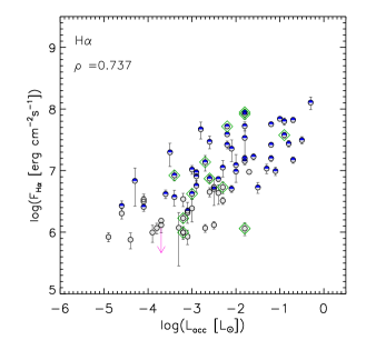
Line fluxes are also very useful for evaluating the mass accretion rate and for comparing it with the one derived from primary indicators, like the Balmer continuum excess. Alcalá et al. (2017) calculated the accretion luminosity, $L_{\rm acc}$ , by modelling the observed flux-calibrated spectra with the sum of a non-accreting (Class III) template and the emission from a slab of hydrogen, which accounts for $L_{\rm acc}$ . The only parameters needed to convert the flux at Earth into luminosity are the distance to the YSO and the extinction.

Mendigutía et al. (2015) suggested that the relations between accretion and line luminosity, $L_{\rm acc}-L_{\rm line}$ , may be the result of the $L_{\rm acc}-L_{\rm*}$ and $L_{\rm line}-L_{\rm*}$ correlations. Indeed, both $L_{\rm acc}$ and $L_{\rm line}$ are obtained adopting the same distance and extinction. Therefore, in their hypothesis, the observed trends may be a “calibration” effect rather than physical correlations.

In the present work we have calculated the line fluxes per unit surface based on the continuum fluxes of the model spectra at the $T_{\rm eff}$ and $\log g$ of the target. Thus, neither the distance nor the extinction enter in the determination of $F_{\rm line}$ .

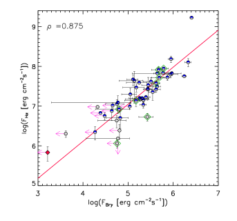
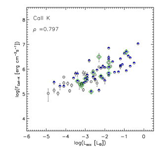
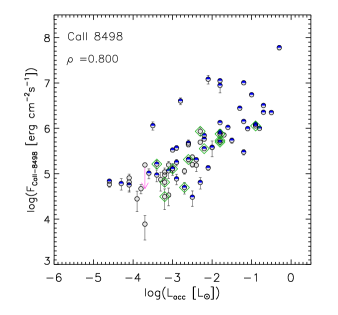
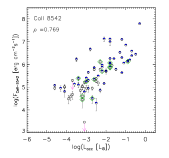
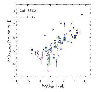
We show in Fig. 15 that line fluxes are highly correlated with the accretion luminosity reported by Alcalá et al. (2017), as also witnessed by the rank-correlation coefficients ranging from 0.59 to 0.80 with significances always smaller than $10^{-6}$ . This excludes a calibration effect and strengthens the validity of the emission lines as accretion diagnostics.

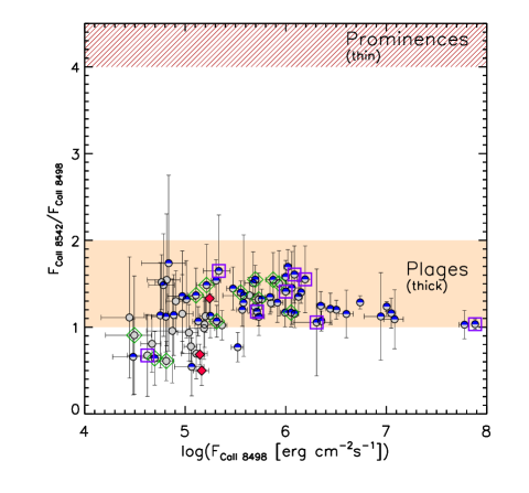
4.5 Flux ratios

The ratio of fluxes in two Ca ii-IRT lines, $F_{\rm CaII8542}/F_{\rm CaII8498}$ , is sensitive to the conditions of the emitting plasma, particularly to its optical depth. It was shown that for optically thick sources, such as dense chromospheric solar or stellar plages, the ratio is typically in the range 1–2; optically-thin emission sources, like solar prominences seen off-limb, have instead large values of this ratio, $F_{\rm CaII8542}/F_{\rm CaII8498}\simeq$ 4–9 (see, e.g., Herbig & Soderblom 1980; Landman 1980, and references therein). As apparent in Fig. 16, the values of this flux ratio are low for all Lupus members in our sample, both Class II and III. This suggests that the bulk of emission is originating in optically-thick regions, either chromospheric plages or the impact regions of accretion flows near the YSOs surface, as already suggested, e.g., by Herbig & Soderblom (1980) and Alcalá et al. (2014).

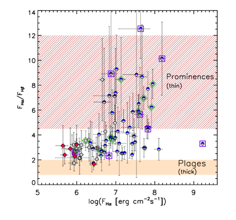
Another indicator of the physical conditions of the emitting matter is the Balmer decrement, which is here defined as the ratio of the H $\alpha$ and H $\beta$ fluxes. We calculated the H $\beta$ flux at the stellar surface in the same way as the H $\alpha$ flux. The Balmer decrement is displayed in Fig. 17. We note that all Class III sources have low values of $F_{\rm H\alpha}/F_{\rm H\beta}$ , which range from about 1.5 to 3. These values are, on average, slightly larger than those typical of solar plages or pre-flare active regions (1–2), but significantly lower than in optically thin regions such as solar prominences observed off limb (e.g., Tandberg-Hanssen 1967; Landman & Mongillo 1979). This behavior was already observed in stars with a very high chromospheric activity level and explained as the result of different physical conditions in the chromospheres or of a combination of plage-like and prominence-like regions in the observed flux (e.g., Hall & Ramsey 1992; Chester et al. 1994; Stelzer et al. 2013).

Several accretors share the same locus of the Class III sources in this diagram, but some others (about one third) display very high values of the Balmer decrement, which indicates a prevalence of optically thin emission in their Balmer lines, similarly to results from other studies of accretors (e.g., Whelan et al. 2014; Frasca et al. 2015; Antoniucci et al. 2017).

This suggests that Ca ii and Balmer lines carry informations about different effects/regions of the accretion process, the former mainly originating in optically thick regions, like, e.g., the impact shocks produced by the accretion flows near the stellar photosphere. The Balmer lines can be formed instead in different parts of the accretion funnels with a large range of optical depth.

We note that the subluminous YSOs, with the exception of SSTc2dJ160703.9-391112, Sz 106 and Sz 102, display large values of the Balmer decrement. This can be understood if we assume that an edge-on disk is the cause of the under-luminosity. In this framework, the densest, and thus optically thickest, regions of the accretion flows are suppressed by the optically thick edge-on disk. Moreover, Antoniucci et al. (2017) report that the whole Balmer series decrement shows a common shape (type 1 in their classification) in most subluminous objects, which is compatible with an edge-on geometry. The rather low values of Balmer decrement for SSTc2dJ160703.9-391112, Sz 106 and Sz 102 may be the result of the geometry of the star/disk system and/or of the strong mass accretion rate, which gives rise to dense flows at rather large distances from the central star.

5 Summary and conclusions

We have presented the results of the analysis of X-Shooter@VLT spectra of 102 YSO candidates, mostly of infrared Class II, in the Lupus star forming region. The application of the code ROTFIT to specific spectral regions at optical and near-infrared wavelengths has allowed us to measure the effective temperature ( $T_{\rm eff}$ ), surface gravity ( $\log g$ ), radial velocity (RV) and projected rotational velocity ( $v\sin i$ ) with median errors of $\sigma_{T_{\rm eff}}=70$ K, $\sigma_{\log g}=0.21$ dex, $\sigma_{\rm RV}=2.3$ km s^-1, and $\sigma_{v\sin i}=4$ km s^-1, respectively. By means of Monte Carlo simulations, we have estimated the minimum detectable $v\sin i$ as 8 km s^-1 with the 0 $\aas@@fstack{\prime\prime}$ 9 VIS slit and 6 km s^-1 with the 0 $\aas@@fstack{\prime\prime}$ 4 VIS slit, respectively. The comparison with the effective temperatures inferred from the spectral classification performed on the same spectra by Manara et al. (2013) and Alcalá et al. (2014, 2017) and with literature data stemming from low-resolution spectroscopy indicates an external accuracy of about 100 K. A similar statistical evaluation cannot be done for the accuracy of $\log g$ and $v\sin i$ , because of the very few values of these parameters available in the literature, which are, however, in good agreement with our determinations. We have also derived the veiling at different wavelengths and confirm previous results that the strongest accretors possess the highest veiling values.

We have shown that 13 candidate members of the Lupus SFR must be definitely considered as non-members on the basis of their discrepant RV with respect to the Lupus SFR and/or the very low $\log g$ values, which suggest that at least 11 of them are background giants in the RGB or AGB phase. Two of them turned out to be lithium-rich giants.

Thanks to the subtraction of inactive template spectra, we have measured the line fluxes corrected for the contribution of the photospheric absorption, even in the objects with the weakest chromospheric or accretion emission. We found that all the Class III sources lie, as expected, in the locus of the $T_{\rm eff}$ - $F_{\rm H\alpha}$ diagram occupied by the objects where chromospheric emission dominates over accretion as defined by Frasca et al. (2015). The Class II sources are mostly above the boundary between chromospheres and accretion, but some of them are also in the domain of the chromospheric sources. However, all the objects fulfilling the White & Basri (2003) criterion, based on the 10% width and EW of the H $\alpha$ emission line, lie, correctly, above the aforementioned boundary, i.e. in the domain of accretors according to Frasca et al. (2015). We do not see any particular trend for the YSOs with transitional disks in this diagram. They display both low and high fluxes similarly to the behavior of their mass accretion rate shown by Alcalá et al. (2017).

The strong correlation between our line fluxes per unit surface and the accretion luminosity ( $L_{\rm acc}$ ) derived by Alcalá et al. (2017) from the Balmer continuum excess has allowed us to confirm the validity of emission lines as accretion diagnostics and to exclude that the relations between $L_{\rm acc}$ and line luminosities are only the result of calibration effects.

We have also investigated the relations between the H $\alpha$ flux and the fluxes in different emission lines (Ca ii IRT, Ca ii K, Na i D, Pa $\gamma$ , Pa $\beta$ , and Br $\gamma$ ). We note that, with the exception of the Class III sources and some of the weak accretors, all the objects display an H $\alpha$ flux in excess to what it is expected from the relations found by Stelzer et al. (2013) for Class III sources. This behavior is likely the result of different physical conditions in the emitting regions of the accretors with respect to chromospheric emitters, which seem to also affect the flux ratios. The latter have been calculated for two Ca ii-IRT lines, $F_{\rm CaII8542}/F_{\rm CaII8498}$ , and for the first two members of the Balmer series, $F_{\rm H\alpha}/F_{\rm H\beta}$ , i.e. the Balmer decrement. We found that the Ca ii-IRT flux ratio takes always small values ( $F_{\rm CaII8542}/F_{\rm CaII8498}<2$ ) that indicate an optically thick emission source. The latter can be identified with the accretion shock near the stellar photosphere. The Balmer decrement takes instead, for several accretors, high values typical of optically thin emission, suggesting that the Balmer emission originates in different parts of the accretion funnels with a smaller optical depth.

Acknowledgements.

We are very grateful to the referee, Fernando Comerón, for his useful comments and suggestions. We thank the ESO staff, in particular Markus Wittkowski and Giacomo Beccari for their excellent support during phase-2 proposal preparation, and the Paranal staff for their support during the observations. We thank G. Cupani, V. D’Odorico, P. Goldoni and A. Modigliani for their help with the X-Shooter pipeline. Financial support from INAF is also acknowledged. CMF acknowledges an ESA Research Fellowship funding. This research made use of the SIMBAD database, operated at the CDS (Strasbourg, France).

References

Alcalá et al. (2006) Alcalá, J. M., Spezzi, L., Frasca, A., et al. 2006, A&A, 453, L1
Alcalá et al. (2011a) Alcalá, J. M., Stelzer, B., Covino, E., et al. 2011a, Astron. Nachr., 332, 242
Alcalá et al. (2011b) Alcalá, J. M., Biazzo, K., Covino, E., Frasca, A., & Bedin, L. R. 2011b, A&A, 531, L12
Alcalá et al. (2014) Alcalá, J. M., Natta, A., Manara, C. F., et al. 2014, A&A, 561, A2
Alcalá et al. (2017) Alcalá, J. M., Manara, C. F., Natta, A., et al. 2017, A&A, 600, A20
Allard et al. (2012) Allard, F., Homeier, D., & Freytag, B. 2012, ASP Conf. Ser., 448, 91
Antoniucci et al. (2017) Antoniucci, S., Nisini, B., Giannini, T., et al. 2017, A&A, 599, A105
Bacciotti et al. (2011) Bacciotti, F., Whelan, E. T., Alcalá, J. M., et al. 2011, ApJ, 737, L26
Baraffe et al. (2015) Baraffe, I., Homeier, D., Allard, F., & Chabrier, G. 2015 A&A, 577, A42
Berdyugina (2009) Berdyugina, S. V. 2009, in Cosmic Magnetic Fields: From Planets to Stars and Galaxies, eds. K. G. Strassmeier, A. G. Kosovichev, and J. E. Beckman, IAU Symp. 259, 323
Bevington (1969) Bevington, P. 1969, in Data Reduction and Error Analysis for the Physical Sciences (New York: Mc Graw-Hill), 237
Biazzo et al. (2016) Biazzo, K., Frasca, A., Alcalá, J. M., et al. 2017, A&A, submitted
Brandenburg et al. (1995) Brandenburg, A., Nordlund, A., Stein, R. F., & Torkelsson, U. 1995, ApJ, 446, 741
Bressan et al. (2012) Bressan, A., Marigo, P., Girardi, L., et al. 2012, MNRAS, 427, 127
Bustamante et al. (2015) Bustamante, I., Merín, B., Ribas, Á., et al. 2015, A&A, 578, A23
Chester et al. (1994) Chester, M. M., Hall, J. C., & Buzasi, D. 1994, in Eigth Cambridge Workshop on Cool Stars Slettar Systems and the Sun, ed. J.-P. Caillault, ASP Conf. Ser., 64, 1994
Calvet et al. (1994) Calvet, N., Hartmann, L., Kenyon, S. J., & Whitney, B. A., 1994, ApJ, 434, 330
Calvet & Gullbring (1998) Calvet, N., & Gullbring, E. 1998, ApJ, 509, 802
Calvet et al. (2004) Calvet, N., Muzerolle, J., Bricen̂o, C., et al. 2004, AJ, 128, 1294
Cardelli et al. (1989) Cardelli, J. A., Clayton, G. C., & Mathis, J. S. 1989, ApJ, 345, 245
Casey et al. (2016) Casey, A. R., Ruchti, G., Masseron, T., et al. 2016, MNRAS, 461, 3336
Claret et al. (2012) Claret, A., Hauschildt, P. H., & Witte, S. 2012, A&A, 546, 14
Cameron & Fowler (1971) Cameron, A. G. W., & Fowler, W. A. 1971, ApJ, 164, 111
Comerón (2008) Comerón, F. 2008 in Handbook of Star Forming Regions, Volume II: The Southern Sky ASP Monograph Publications, Vol. 5, Edited by Bo Reipurth, p. 295
Comerón et al. (2009) Comerón, F., Spezzi, L., & López Martí, B. 2009, A&A, 500, 1045
Comerón et al. (2013) Comerón, F., Spezzi, L., López Martí, B., & Merín, B. 2013, A&A, 554, A86
Costigan et al. (2012) Costigan, G., Scholz, A., Stelzer, B., et al. 2012, MNRAS, 427, 1344
Dubath et al. (1996) Dubath, P., Reipurth, B., & Mayor, M. 1996, A&A, 308, 107
Evans et al. (2009) Evans, N. J. II, Dunham, M. M., Jörgensen, J. K., et al. 2009, ApJS, 181, 321
Facchini et al. (2016) Facchini, S., Manara, C. F., Schneider, P. C., et al. 2016, 596, 38
Feigelson & Montmerle (1999) Feigelson, E. D., & Montmerle, T. 1999, ARA&A, 37, 363
Fischer et al. (2011) Fischer, W., Edwards, S., Hillenbrand, L., & Kwan, J. 2011, ApJ, 730, 73
Frasca & Catalano (1994) Frasca, A., & Catalano, S. 1994, A&A, 284, 883
Frasca et al. (2006) Frasca, A., Guillout, P., Marilli, E., et al. 2006, A&A, 454, 301
Frasca et al. (2015) Frasca, A., Biazzo, K., Lanzafame, A. C., et al. 2015, A&A, 575, A4
Frasca et al. (2016) Frasca, A., Molenda-Żakowicz, J., De Cat, P., et al. 2016, A&A, 594, A39
Galli et al. (2013) Galli, P. A. B., Bertout, C., Teixeira, R., & Ducouran, C. 2013, A&A, 558, A77
Glebocki & Gnacinski (2005) Glebocki, R., & Gnacinski, P. 2005, ESA, SP-560, 571
Gomes da Silva et al. (2011) Gomes da Silva, J., Santos, N. C., Bonfils, X., et al. 2011, A&A, 534, A30
Gray (2005) Gray, D. F. 2005, The Observation and Analysis of Stellar Photospheres, (Cambridge: Cambridge University Press)
Hall & Ramsey (1992) Hall, J. C., & Ramsey, L. W. 1992, AJ, 104, 1942
Hartigan et al. (1991) Hartigan, P., Kenyon, S. J., Hartmann, L., et al. 1991, ApJ, 382, 617
Hartmann et al. (1994) Hartmann, L., Hewett, R., & Calvet, N. 1994, ApJ, 426, 669
Hartmann et al. (2016) Hartmann, L., Herczeg, G., & Calvet, N. 2016, ARA&A, 54, 135
Hawley & Balbus (1991) Hawley, J. F., & Balbus, S. A. 1991, ApJ, 376, 223
Herbig & Soderblom (1980) Herbig, G. H., & Soderblom, D. R. 1980, ApJ, 242, 628
Herczeg & Hillenbrand (2008) Herczeg, G. J., & Hillenbrand, L. A. 2008, ApJ, 681, 594
Herczeg & Hillenbrand (2014) Herczeg, G. J., & Hillenbrand, L. A. 2014, ApJ, 786, 97
Houdebine et al. (2009) Houdebine, E. R., Junghans, K., Heanue, M. C., & Andrews, A. D. 2009, A&A, 503, 929
Kenyon & Hartmannn (1995) Kenyon, S., & Hartmann, L. 1995, ApJ, 101, 117
Kurosawa et al. (2011) Kurosawa, R., Romanova, M. M., & Harries, T. J. 2011, MNRAS, 416, 2623
Landman & Mongillo (1979) Landman, D. A., & Mongillo, M. 1979, ApJ, 230, 581
Landman (1980) Landman, D. A. 1980, ApJ, 237, 988
Larson (2003) Larson, R. B. 2003, Rep. Progr. Phys., 66, 1651
Luhman et al. (2003) Luhman, K. L., Stauffer, J., Muench, A., et al. 2003, ApJ, 593, 1093
Manara et al. (2013) Manara, C. F., Testi, L., Rigliaco, E., et al. 2013, A&A, 551, A107
Martínez-Arnáiz et al. (2011) Martínez-Arnáiz, R., López-Santiago, J., Crespo-Chacón, I., & Montes, D. 2011, MNRAS, 414, 2629
Mendigutía et al. (2015) Mendigutía, I., Oudmaijer, R. D., Rigliaco, E., et al. 2015, MNRAS, 452, 2837
Merín et al. (2008) Merín, B., Jørgensen, J., Spezzi, L., et al. 2008, ApJS, 177, 551
Modigliani et al. (2010) Modigliani, A., Goldoni, P., Royer, F., et al. 2010, in Observatory Operations: Strategies, Processes, and Systems III, eds. D. R. Silva, A. B. Peck, & B. T. Soifer, SPIE, 7737
Mohanty et al. (2005) Mohanty, S., Jayawardhana, R., & Basri, G. 2005, ApJ, 626, 498
Montes et al. (1995) Montes, D., de Castro, E., Fernández-Figueroa, M. J., & Cornide, M. 1995, A&AS, 114, 287
Montes et al. (2001) Montes, D., López-Santiago, J., Fernández-Figueroa, M. J., & Gálvez, M. C. 2001, A&A, 379, 976
Muzerolle et al. (1998) Muzerolle, J., Hartmann, L., & Calvet, N. 1998, AJ, 116, 2965
Muzerolle et al. (2003) Muzerolle, J., Hillenbrand, L., Calvet, N., Briceño, C., Hartmann, L. 2003, ApJ, 592, 266
Muzic et al. (2014) Muzic, K., Scholz, A., Geers, V. C., Jayawardhana, R., & López Martí, B., 2014, ApJ, 785, 159
Natta & Giovanardi (1990) Natta, A., & Giovanardi, C. 1990, ApJ, 356, 646
Natta et al. (2014) Natta, A., Testi, L., Alcalá, J. M., et al. 2014, A&A, 569, A5
Pecaut & Mamajek (2013) Pecaut, M. J., & Mamajek, E. E. 2013, ApJS, 208, 9
Press et al. (1992) Press, W. H., Teukolsky, S. A., Vetterling, W. T., & Flannery, B. P. 1992, Numerical Recipes in Fortran (2d ed; Cambridge: Cambridge Univ. Press)
Rigliaco et al. (2012) Rigliaco, E., Natta, A., Testi, L., et al. 2012, A&A, 548, A56
Siess et al. (2000) Siess, L., Dufour, E., & Forestini, M. 2000, A&A, 385, 593
Smiljanic et al. (2016) Smiljanic, R., Franciosini, E., Randich, S., et al. 2016, A&A, 591, A62
Stelzer et al. (2013) Stelzer, B., Frasca, A., Alcalá, et al. 2013, A&A, 558, A141
Strassmeier et al. (2000) Strassmeier, K. G., Washuettl, A., Granzer, Th., Scheck, M., & Weber, M. 2000, A&AS, 142, 275
Tandberg-Hanssen (1967) Tandberg-Hanssen, E. 1967, Solar activity, Waltham, Mass.: Blaisdell
Torres et al. (2006) Torres, C. A. O., Quast, G. R., da Silva, L., et al. 2006, A&A, 460, 695
Vernet et al. (2011) Vernet, J., Dekker, H., D’Odorico, S., Kaper, L., et al. 2011, A&A, 536, 105
Whelan et al. (2014) Whelan, E. T., Alcalá, J. M., Bacciotti, F., et al. 2014, A&A, 570, A59
White & Basri (2003) White, R. J., & Basri, G. 2003, ApJ, 582, 1109

Table 1: Stellar parameters.

Name	HJD	Memb/	$T_{\rm eff}$	$\sigma_{T_{\rm eff}}$	$\log g$	err	$v\sin i$	err	RV	err	$r_{970}$	$r_{710}$	$r_{620}$	$r_{540}$	$r_{450}$	$M_{\ast}$	Age
	(-2 450 000)	class	(K)		(dex)		(km s^-1)		(km s^-1)							( $M_{\sun}$ )	(Myr)
Sz 66	6035.7578	Y/II	3351	47	3.81	0.21	$\leq$ 8.0	…	2.4	1.8	$\leq$ 0.2	$\leq$ 0.2	0.8	1.5	2.0	0.30	3.9
AKC2006 19	5674.7067	Y/II	3027	34	4.45	0.11	$\leq$ 8.0	…	9.6	2.1	$\leq$ 0.2	$\leq$ 0.2	$\leq$ 0.2	…	…	0.09	8.0
Sz 69	5674.6058	Y/II	3163	119	3.50	0.23	33.0	4.0	5.4	2.9	$\leq$ 0.2	$\leq$ 0.2	$\leq$ 0.2	…	…	0.20	2.6
Sz 71	6035.6010	Y/II	3599	35	4.27	0.24	$\leq$ 8.0	…	-3.3	1.9	$\leq$ 0.2	0.3	0.5	0.6	0.6	0.40	2.0
Sz 72	6035.6987	Y/II	3550	70	4.18	0.28	$\leq$ 8.0	…	6.9	2.4	$\leq$ 0.2	$\leq$ 0.2	$\leq$ 0.2	…	…	0.40	2.9
Sz 73	6035.7983	Y/II	3980	33	4.40	0.33	31.0	3.0	5.0	2.2	$\leq$ 0.2	0.5	1.0	1.0	0.5	0.70	3.7
Sz 74	6035.6747	Y/II	3371	79	3.98	0.11	30.2	1.0	1.0	1.5	$\leq$ 0.2	$\leq$ 0.2	0.4	0.7	0.8	0.30	0.5
Sz 83	6035.6842	Y/II	4037	96	3.5	0.4	8.5	4.8	3.3	1.8	1.4	2.4	3.5	…	…	0.70	0.8
Sz 84	6035.6145	Y/II	3058	82	4.20	0.21	21.3	4.1	-3.1	2.0	$\leq$ 0.2	$\leq$ 0.2	0.3	0.9	1.5	0.10	1.8
Sz 130	5293.8661	Y/II	3448	62	4.48	0.10	$\leq$ 8.0	…	3.6	2.6	$\leq$ 0.2	$\leq$ 0.2	0.7	…	…	0.30	2.3
Sz 88 A	6035.8400	Y/II	3700	19	3.77	0.47	$\leq$ 8.0	…	6.5	2.3	0.4	1.4	2.1	…	…	0.50	4.0
Sz 88 B	6035.8400	Y/II	3075	111	4.08	0.12	$\leq$ 8.0	…	5.7	2.1	$\leq$ 0.2	0.3	0.3	…	…	0.20	2.0
Sz 91	6035.8270	Y/II	3664	45	4.34	0.22	$\leq$ 8.0	…	4.0	2.4	$\leq$ 0.2	0.4	0.6	0.9	0.9	0.40	1.5
Lup 713	5292.7036	Y/II	2943	109	3.89	0.13	24.0	4.0	3.9	3.3	$\leq$ 0.2	$\leq$ 0.2	…	…	…	0.08	4.7
Lup 604s	5292.7434	Y/II	3014	62	3.89	0.12	31.5	2.8	2.7	1.9	$\leq$ 0.2	$\leq$ 0.2	$\leq$ 0.2	…	…	0.10	2.2
Sz 97	5674.6202	Y/II	3185	78	4.14	0.16	25.1	1.5	2.4	2.2	$\leq$ 0.2	$\leq$ 0.2	$\leq$ 0.2	0.7	0.9	0.20	1.3
Sz 99	5293.8505	Y/II	3297	98	3.89	0.21	38.0	3.0	3.2	3.1	$\leq$ 0.2	$\leq$ 0.2	$\leq$ 0.2	…	…	0.30	7.5
Sz 100	5674.6454	Y/II	3037	44	3.87	0.21	16.6	5.4	2.7	2.5	$\leq$ 0.2	$\leq$ 0.2	$\leq$ 0.2	…	…	0.10	4.7
Sz 103	5674.6604	Y/II	3380	36	3.97	0.10	12.0	4.0	1.4	2.2	$\leq$ 0.2	$\leq$ 0.2	0.3	0.7	0.7	0.30	3.3
Sz 104	5292.7601	Y/II	3074	73	3.96	0.10	$\leq$ 8.0	…	2.3	2.3	$\leq$ 0.2	$\leq$ 0.2	$\leq$ 0.2	…	…	0.20	2.4
Lup 706	5292.7882	Y/II	2750	82	3.93	0.11	25.0	15.0	11.9	4.5	$\leq$ 0.2	$\leq$ 0.2	…	…	…	…^a	…^a
Sz 106	6035.8117	Y/II	3691	35	4.82	0.13	$\leq$ 8.0	…	8.0	2.6	$\leq$ 0.2	$\leq$ 0.2	0.5	0.5	0.5	…^a	…^a
Par-Lup3-3	5292.8638	Y/II	3461	49	4.47	0.11	$\leq$ 8.0	…	3.5	2.5	$\leq$ 0.2	$\leq$ 0.2	$\leq$ 0.2	…	…	0.30	1.5
Par-Lup3-4	5293.6849	Y/II	3089	246	3.56	0.80	12.0	10.0	5.6	4.3	0.3	0.3	…	…	…	…^a	…^a
Sz 110	5674.8476	Y/II	3215	162	4.31	0.21	$\leq$ 8.0	…	2.6	2.3	0.4	0.4	1.0	2.7	3.3	0.20	0.6
Sz 111	6035.6286	Y/II	3683	34	4.66	0.21	$\leq$ 8.0	…	-1.2	2.1	$\leq$ 0.2	0.3	0.5	0.6	0.6	0.50	4.2
Sz 112	6035.7704	Y/II	3079	47	3.96	0.10	$\leq$ 8.0	…	6.2	1.7	$\leq$ 0.2	$\leq$ 0.2	$\leq$ 0.2	…	…	0.10	11.3
Sz 113	5674.8663	Y/II	3064	114	3.76	0.27	$\leq$ 8.0	…	6.1	2.4	0.3	0.5	…	…	…	0.10	1.8
2MASS J16085953-3856275	5674.7905	Y/II	2649	31	3.98	0.10	$\leq$ 8.0	…	7.2	4.0	$\leq$ 0.2	$\leq$ 0.2	$\leq$ 0.2	…	…	0.025	1.0
SSTc2d160901.4-392512	5674.7331	Y/II	3305	57	4.51	0.11	$\leq$ 8.0	…	15.9	0.7	$\leq$ 0.2	$\leq$ 0.2	$\leq$ 0.2	0.7	0.6	0.30	6.1
Sz 114	5674.8913	Y/II	3134	35	3.92	0.12	$\leq$ 8.0	…	4.0	2.4	$\leq$ 0.2	0.3	0.3	0.6	0.8	0.20	2.4
Sz 115	6035.8529	Y/II	3124	42	3.90	0.21	9.2	6.3	6.4	2.3	$\leq$ 0.2	$\leq$ 0.2	$\leq$ 0.2	…	…	0.20	2.3
Lup 818s	5674.7539	Y/II	2953	59	3.97	0.11	12.4	6.0	5.1	2.0	$\leq$ 0.2	$\leq$ 0.2	$\leq$ 0.2	…	…	0.08	4.2
Sz123 A	6035.7844	Y/II	3521	70	4.46	0.13	12.3	3.0	1.8	1.8	$\leq$ 0.2	$\leq$ 0.2	0.6	1.2	1.2	0.40	4.4
Sz123 B	6035.8971	Y/II	3513	45	4.17	0.22	$\leq$ 8.0	…	7.4	2.3	$\leq$ 0.2	$\leq$ 0.2	0.6	0.8	0.9	…^a	…^a
SST-Lup3-1	5292.8841	Y/II	3042	43	3.95	0.11	$\leq$ 8.0	…	6.3	2.6	$\leq$ 0.2	$\leq$ 0.2	$\leq$ 0.2	…	…	0.10	3.2
Sz 65	7177.5239	Y/II	4005	75	3.85	0.26	$\leq$ 8.0	…	-2.7	2.0	$\leq$ 0.2	$\leq$ 0.2	0.3	0.3	$\leq$ 0.2	0.70	1.9
AKC2006 18	7132.7794	Y/II	2930	45	4.46	0.11	$\leq$ 8.0	…	9.1	2.3	$\leq$ 0.2	$\leq$ 0.2	$\leq$ 0.2	…	…	0.07	8.3
SSTc2dJ154508.9-341734	7188.6599	Y/II	3242	205	3.33	0.77	$\leq$ 8.0	…	-0.8	2.7	0.6	0.7	0.8	…	…	0.20	4.8
Sz 68	7160.7168	Y/II	4506	82	3.68	0.12	39.6	1.2	-4.3	1.8	0.3	0.3	0.3	0.3	0.3	1.20	0.5
SSTc2dJ154518.5-342125	7199.4886	Y/II	2700	100	3.45	0.11	13.0	6.0	4.4	2.9	$\leq$ 0.2	$\leq$ 0.2	$\leq$ 0.2	…	…	0.07	0.5
Sz 81 A	7253.5752	Y/II	3077	151	3.48	0.11	$\leq$ 8.0	…	-0.1	2.9	$\leq$ 0.2	$\leq$ 0.2	0.3	…	…	0.20	1.0
Sz 81 B	7253.5752	Y/II	2991	76	3.53	0.11	25.0	5.0	1.2	2.4	$\leq$ 0.2	$\leq$ 0.2	0.3	…	…	0.10	1.7
Sz 129	7199.5644	Y/II	4005	45	4.49	0.25	$\leq$ 10.0	…	3.2	2.5	$\leq$ 0.2	$\leq$ 0.2	1.0	1.4	1.1	0.70	3.5
SSTc2dJ155925.2-423507	7200.5241	Y/II	2984	82	4.41	0.12	$\leq$ 8.0	…	6.5	2.5	$\leq$ 0.2	$\leq$ 0.2	$\leq$ 0.2	…	…	0.09	5.8
RY Lup	7205.7799	Y/II	5082	118	3.87	0.22	16.3	5.3	1.3	2.0	0.3	$\leq$ 0.2	0.5	0.4	$\leq$ 0.2	1.40	10.2
SSTc2dJ160000.6-422158	7115.8505	Y/II	3086	82	4.03	0.11	$\leq$ 8.0	…	2.5	2.2	$\leq$ 0.2	$\leq$ 0.2	$\leq$ 0.2	…	…	0.20	2.6
SSTc2dJ160002.4-422216	7204.6729	Y/II	3159	140	4.00	0.48	$\leq$ 8.0	…	2.6	2.6	$\leq$ 0.2	$\leq$ 0.2	$\leq$ 0.2	0.3	0.3	0.20	1.5
SSTc2dJ160026.1-415356	7201.5176	Y/II	2976	221	3.97	0.35	$\leq$ 8.0	…	-1.1	2.3	$\leq$ 0.2	$\leq$ 0.2	0.3	…	…	0.10	1.6
MY Lup	7199.5763	Y/II	4968	200	3.72	0.18	29.1	2.0	4.4	2.1	$\leq$ 0.2	$\leq$ 0.2	$\leq$ 0.2	$\leq$ 0.2	$\leq$ 0.2	1.10	16.6
Sz 131	7204.7286	Y/II	3300	122	4.29	0.36	$\leq$ 8.0	…	2.4	2.2	$\leq$ 0.2	$\leq$ 0.2	0.3	…	…	0.20	1.6
Sz 133	7205.7011	Y/II	4420	129	3.96	0.51	$\leq$ 8.0	…	0.7	2.5	0.5	0.5	0.7	0.7	0.7	…^a	…^a
SSTc2dJ160703.9-391112	7542.7095	Y/II	3072	55	4.01	0.11	$\leq$ 8.0	…	1.8	2.7	$\leq$ 0.2	$\leq$ 0.2	$\leq$ 0.2	…	…	…^a	…^a
SSTc2dJ160708.6-391408	7545.5860	Y/II	3474	206	4.18	0.56	$\leq$ 8.0	…	-4.2	2.9	0.7	0.9	1.0	…	…	0.30^b	3.0^b
Sz 90	7215.6018	Y/II	4022	52	4.24	0.42	$\leq$ 8.0	…	1.6	2.3	$\leq$ 0.2	$\leq$ 0.2	0.5	0.5	0.5	0.70	2.1
Sz 95	7215.6243	Y/II	3443	53	4.37	0.12	$\leq$ 8.0	…	-2.8	2.3	$\leq$ 0.2	$\leq$ 0.2	$\leq$ 0.2	…	…	0.30	0.8
Sz 96	7206.7765	Y/II	3702	57	4.50	0.23	$\leq$ 8.0	…	-2.7	2.6	$\leq$ 0.2	$\leq$ 0.2	0.4	0.3	0.3	0.40	0.6
2MASSJ16081497-3857145	7132.8450	Y/II	3024	46	3.96	0.23	22.0	4.2	6.0	2.9	$\leq$ 0.2	$\leq$ 0.2	$\leq$ 0.2	…	…	0.09	15.2
Sz 98	7205.6379	Y/II	4080	71	4.10	0.23	$\leq$ 8.0	…	-1.4	2.1	0.3	0.3	0.6	0.5	0.5	0.70	0.5
Lup 607	7165.7248	Y/II	3084	46	4.48	0.11	$\leq$ 8.0	…	6.8	2.4	$\leq$ 0.2	$\leq$ 0.2	$\leq$ 0.2	…	…	0.10	5.8
Sz 102	7129.8096	Y/II	5145	50	4.10	0.50	41.0	2.8	21.6	12.4	1.0	2.0	2.5	…	…	…^a	…^a
SSTc2dJ160830.7-382827	7205.6604	Y/II	4797	145	4.09	0.23	$\leq$ 8.0	…	1.2	1.9	$\leq$ 0.2	$\leq$ 0.2	$\leq$ 0.2	0.1	$\leq$ 0.2	1.80*	2.9*
SSTc2dJ160836.2-392302	7522.7342	Y/II	4429	83	4.04	0.13	$\leq$ 8.0	…	2.2	2.1	$\leq$ 0.2	$\leq$ 0.2	0.3	0.3	$\leq$ 0.2	1.10	1.3
Sz 108 B	7191.6713	Y/II	3102	59	3.86	0.22	$\leq$ 8.0	…	0.2	2.2	$\leq$ 0.2	$\leq$ 0.2	$\leq$ 0.2	…	…	0.20	2.3
2MASSJ16085324-3914401	7215.6425	Y/II	3393	85	4.24	0.41	$\leq$ 8.0	…	0.9	2.2	$\leq$ 0.2	$\leq$ 0.2	0.3	…	…	0.30	1.1
2MASSJ16085373-3914367	7165.7974	Y/II	2840	200	3.60	0.45	$\leq$ 8.0	…	6.1	6.9	$\leq$ 0.2	$\leq$ 0.2	$\leq$ 0.2	…	…	0.07	13.8
2MASSJ16085529-3848481	7215.6660	Y/II	2899	55	3.99	0.11	$\leq$ 8.0	…	-1.1	2.4	$\leq$ 0.2	$\leq$ 0.2	$\leq$ 0.2	…	…	0.09	0.7
SSTc2dJ160927.0-383628	7216.5318	Y/II	3147	58	4.00	0.10	$\leq$ 8.0	…	3.4	2.2	0.5	0.5	1.5	…	…	0.20	2.2
Sz 117	7216.5747	Y/II	3470	51	4.10	0.32	$\leq$ 8.0	…	-1.4	2.2	$\leq$ 0.2	$\leq$ 0.2	0.4	0.7	0.7	0.30	0.7
Sz 118	7216.6035	Y/II	4067	82	4.47	0.37	$\leq$ 8.0	…	-0.8	2.3	$\leq$ 0.2	$\leq$ 0.2	0.5	0.5	0.5	0.70	1.0
2MASSJ16100133-3906449	7216.6318	Y/II	3018	72	3.77	0.23	15.9	5.4	0.1	2.6	$\leq$ 0.2	$\leq$ 0.2	$\leq$ 0.2	…	…	0.10	1.8
SSTc2dJ161018.6-383613	7252.5473	Y/II	3012	48	3.98	0.10	$\leq$ 8.0	…	-0.2	2.5	$\leq$ 0.2	$\leq$ 0.2	$\leq$ 0.2	…	…	0.10	2.6
SSTc2dJ161019.8-383607	7242.5936	Y/II	2861	69	4.00	0.10	25.0	7.0	1.8	2.5	$\leq$ 0.2	$\leq$ 0.2	$\leq$ 0.2	…	…	0.09	0.5
SSTc2dJ161029.6-392215	7247.5973	Y/II	3098	59	4.02	0.10	13.0	4.0	-2.7	2.2	$\leq$ 0.2	$\leq$ 0.2	$\leq$ 0.2	…	…	0.20	2.0
SSTc2dJ161243.8-381503	7213.6804	Y/II	3687	22	4.57	0.21	$\leq$ 8.0	…	-2.3	2.4	$\leq$ 0.2	$\leq$ 0.2	0.3	…	…	0.40	0.5
SSTc2dJ161344.1-373646	7200.4846	Y/II	3028	78	4.25	0.14	$\leq$ 8.0	…	-1.2	2.3	$\leq$ 0.2	0.3	0.5	…	…	0.10	1.8

Table 1: Continued.

Name	HJD	Memb/	$T_{\rm eff}$	$\sigma_{T_{\rm eff}}$	$\log g$	err	$v\sin i$	err	RV	err	$r_{970}$	$r_{710}$	$r_{620}$	$r_{540}$	$r_{450}$	$M_{\ast}$	Age
	(-2 450 000)	Class	(K)		(dex)		(km s^-1)		(km s^-1)							( $M_{\sun}$ )	(Myr)
GQ Lup	5321.7673	Y/II	4192	65	4.12	0.36	$\leq$ 6.0	…	-3.6	1.3	0.3	0.3	0.5	0.8	0.6	0.80	0.9
Sz 76	6775.7518	Y/II	3440	60	4.41	0.26	$\leq$ 6.0	…	1.4	1.0	$\leq$ 0.2	$\leq$ 0.2	$\leq$ 0.2	0.7	0.6	0.30	2.3
Sz 77	5321.8825	Y/II	4131	48	4.28	0.31	6.7	1.5	2.4	1.5	$\leq$ 0.2	$\leq$ 0.2	0.4	0.5	0.3	0.80	3.0
RXJ1556.1-3655	6775.7703	Y/II	3770	70	4.75	0.21	12.7	1.3	2.6	1.2	$\leq$ 0.2	0.3	1.4	…	…	0.60	7.8
IM Lup	5320.5707	Y/II	4146	95	3.80	0.37	17.1	1.4	-0.5	1.3	$\leq$ 0.2	$\leq$ 0.2	$\leq$ 0.2	$\leq$ 0.2	$\leq$ 0.2	0.70	0.5
EX Lup	5320.6616	Y/II	3859	62	4.31	0.29	7.5	1.9	1.9	1.4	0.4	$\leq$ 0.2	0.7	1.0	0.7	0.50	0.5
Sz 94	5292.7286	Y/III	3205	59	4.21	0.24	38.0	3.0	7.8	2.0	$\leq$ 0.2	$\leq$ 0.2	$\leq$ 0.2	…	…	0.20	1.3
Par Lup3 1	5293.8248	Y/III	2766	77	3.48	0.11	31.0	7.0	4.9	3.9	$\leq$ 0.2	$\leq$ 0.2	$\leq$ 0.2	…	…	0.08	0.5
Par Lup3 2	5292.8383	Y/III	3060	61	3.91	0.24	33.0	5.0	5.0	2.5	$\leq$ 0.2	$\leq$ 0.2	$\leq$ 0.2	…	…	0.10	1.8
Sz 107	5674.6759	Y/III	2928	100	3.52	0.13	66.6	4.1	6.1	3.8	$\leq$ 0.2	$\leq$ 0.2	$\leq$ 0.2	…	…	0.10	0.5
Sz 108 A	7191.6832	Y/III	3676	34	4.50	0.21	$\leq$ 8.0	…	0.4	2.2	$\leq$ 0.2	$\leq$ 0.2	0.4	0.5	0.3	0.40	1.0
Sz 121	6035.6419	Y/III	3178	61	4.08	0.12	87.0	8.0	-0.9	4.4	$\leq$ 0.2	$\leq$ 0.2	$\leq$ 0.2	…	…	0.20	0.5
Sz 122	6035.7433	Y/III	3511	27	4.58	0.21	149.2	1.0	2.9	3.0	$\leq$ 0.2	$\leq$ 0.2	$\leq$ 0.2	…	…	0.40	6.8
Sz 78	7199.5386	N^c	4347	119	2.04	0.23	$\leq$ 8.0	…	1.8	2.0	$\leq$ 0.2	$\leq$ 0.2	$\leq$ 0.2	$\leq$ 0.2	$\leq$ 0.2	…	…
Sz 79	7199.5523	N^c	4718	147	2.44	0.22	19.3	2.1	-84.6	1.8	$\leq$ 0.2	$\leq$ 0.2	$\leq$ 0.2	…	…	…	…
IRAS15567-4141	7205.6767	N^c	3130	135	2.83	0.45	30.0	14.0	-43.0	8.2	$\leq$ 0.2	$\leq$ 0.2	$\leq$ 0.2	…	…	…	…
SSTc2dJ160034.4-422540	7204.7102	N^c	2050	150	…	…	…	…	-84.5	4.3	…	…	…	…	…	…	…
SSTc2dJ160708.6-394723	7206.7441	N^c	4647	104	2.64	0.23	10.1	1.0	-70.7	1.8	$\leq$ 0.2	$\leq$ 0.2	$\leq$ 0.2	$\leq$ 0.2	$\leq$ 0.2	…	…
Sz 92	7205.7363	N^d	4926	111	2.29	0.26	$\leq$ 8.0	…	-34.8	2.3	$\leq$ 0.2	$\leq$ 0.2	$\leq$ 0.2	$\leq$ 0.2	$\leq$ 0.2	…	…
2MASSJ16080618-3912225	7132.9002	N^c	2753	130	2.02	0.88	13.0	6.0	-57.5	8.2	$\leq$ 0.2	$\leq$ 0.2	$\leq$ 0.2	…	…	…	…
Sz 105	6035.6593	N^c	3187	102	0.76	0.58	14.3	7.8	4.7	1.1	0.4	0.4	0.5	…	…	…	…
SSTc2dJ161045.4-385455	7545.5166	N^c	5114	514	3.40	0.90	42.6	2.3	-115.1	3.1	$\leq$ 0.2	$\leq$ 0.2	$\leq$ 0.2	$\leq$ 0.2	$\leq$ 0.2	…	…
SSTc2dJ161148.7-381758	7116.8337	N^c	6877	143	3.91	0.58	23.1	2.4	-47.6	2.5	$\leq$ 0.2	$\leq$ 0.2	$\leq$ 0.2	$\leq$ 0.2	$\leq$ 0.2	…	…
SSTc2dJ161211.2-383220	7520.7096	N^c	3401	37	1.35	0.41	19.0	15.0	-80.2	1.8	$\leq$ 0.2	$\leq$ 0.2	$\leq$ 0.2	…	…	…	…
SSTc2dJ161222.7-371328	7177.5451	N^c	3321	79	0.99	0.23	$\leq$ 8.0	…	8.4	1.8	$\leq$ 0.2	$\leq$ 0.2	$\leq$ 0.2	$\leq$ 0.2	$\leq$ 0.2	…	…
SSTc2dJ161256.0-375643	7205.7677	N^d	3544	66	0.54	0.25	19.0	4.0	-112.5	1.8	$\leq$ 0.2	$\leq$ 0.2	$\leq$ 0.2	$\leq$ 0.2	$\leq$ 0.2	…	…

* Mass and age derived from Siess et al. (2000) evolutionary models.
^a Subluminous objects.
^b Flat IR source (Merín et al. 2008). Subluminous with the “optical” luminosity. Mass and age derived adopting the bolometric luminosity of 0.18 $L_{\sun}$ (Evans et al. 2009).
^c Originally selected as Class II.
^d Originally selected as Class III.

Table 2: H

\alpha

, H

\beta

, Ca ii, and Na i D_1,2 fluxes.

Name	$10\%W_{\rm H\alpha}$	err	$F_{\rm H\alpha}$	err	$F_{\rm H\beta}$	err	$F_{\rm CaII8498}$	err	$F_{\rm CaII8542}$	err	$F_{\rm CaII8662}$	err	$F_{\rm CaII-K}$	err	$F_{\rm NaI-D_{2}}$	err	$F_{\rm NaI-D_{1}}$	err
	(km s^-1)		(erg cm^-2s^-1)		(erg cm^-2s^-1)		(erg cm^-2s^-1)		(erg cm^-2s^-1)		(erg cm^-2s^-1)		(erg cm^-2s^-1)		(erg cm^-2s^-1)		(erg cm^-2s^-1)
Sz66	475.4	22.8	1.58 $\cdot 10^{7}$	1.94 $\cdot 10^{6}$	3.08 $\cdot 10^{6}$	3.93 $\cdot 10^{5}$	8.26 $\cdot 10^{5}$	1.14 $\cdot 10^{5}$	1.06 $\cdot 10^{6}$	1.19 $\cdot 10^{5}$	1.01 $\cdot 10^{6}$	1.20 $\cdot 10^{5}$	5.62 $\cdot 10^{5}$	3.04 $\cdot 10^{4}$	1.53 $\cdot 10^{5}$	4.68 $\cdot 10^{4}$	1.00 $\cdot 10^{5}$	3.85 $\cdot 10^{4}$
AKC2006 19	228.5	45.7	2.57 $\cdot 10^{6}$	3.94 $\cdot 10^{5}$	8.91 $\cdot 10^{5}$	1.41 $\cdot 10^{5}$	5.66 $\cdot 10^{4}$	1.74 $\cdot 10^{4}$	6.43 $\cdot 10^{4}$	2.81 $\cdot 10^{4}$	5.43 $\cdot 10^{4}$	1.74 $\cdot 10^{4}$	2.03 $\cdot 10^{5}$	2.12 $\cdot 10^{4}$	1.23 $\cdot 10^{4}$	9.10 $\cdot 10^{3}$	1.39 $\cdot 10^{4}$	1.22 $\cdot 10^{4}$
Sz69	411.4	13.7	4.69 $\cdot 10^{7}$	1.43 $\cdot 10^{7}$	5.41 $\cdot 10^{6}$	2.03 $\cdot 10^{6}$	4.01 $\cdot 10^{6}$	6.74 $\cdot 10^{5}$	4.62 $\cdot 10^{6}$	7.76 $\cdot 10^{5}$	4.00 $\cdot 10^{6}$	6.73 $\cdot 10^{5}$	2.22 $\cdot 10^{6}$	3.03 $\cdot 10^{5}$	4.97 $\cdot 10^{5}$	2.86 $\cdot 10^{5}$	3.74 $\cdot 10^{5}$	2.18 $\cdot 10^{5}$
Sz71	356.5	9.2	3.88 $\cdot 10^{7}$	2.73 $\cdot 10^{6}$	5.97 $\cdot 10^{6}$	5.69 $\cdot 10^{5}$	5.78 $\cdot 10^{5}$	3.64 $\cdot 10^{4}$	7.64 $\cdot 10^{5}$	4.62 $\cdot 10^{4}$	5.75 $\cdot 10^{5}$	3.23 $\cdot 10^{4}$	1.10 $\cdot 10^{6}$	4.08 $\cdot 10^{4}$	2.41 $\cdot 10^{5}$	3.51 $\cdot 10^{4}$	1.83 $\cdot 10^{5}$	2.81 $\cdot 10^{4}$
Sz72	457.1	9.1	5.27 $\cdot 10^{7}$	8.88 $\cdot 10^{6}$	1.78 $\cdot 10^{7}$	3.37 $\cdot 10^{6}$	1.12 $\cdot 10^{7}$	1.18 $\cdot 10^{6}$	1.30 $\cdot 10^{7}$	1.37 $\cdot 10^{6}$	1.05 $\cdot 10^{7}$	1.11 $\cdot 10^{6}$	7.11 $\cdot 10^{6}$	4.17 $\cdot 10^{5}$	1.79 $\cdot 10^{6}$	4.70 $\cdot 10^{5}$	1.32 $\cdot 10^{6}$	3.55 $\cdot 10^{5}$
Sz73	502.8	9.2	6.91 $\cdot 10^{7}$	3.65 $\cdot 10^{6}$	1.50 $\cdot 10^{7}$	1.04 $\cdot 10^{6}$	5.50 $\cdot 10^{6}$	2.37 $\cdot 10^{5}$	7.07 $\cdot 10^{6}$	2.83 $\cdot 10^{5}$	5.39 $\cdot 10^{6}$	2.27 $\cdot 10^{5}$	4.30 $\cdot 10^{6}$	2.24 $\cdot 10^{5}$	4.86 $\cdot 10^{5}$	1.08 $\cdot 10^{5}$	3.24 $\cdot 10^{5}$	9.61 $\cdot 10^{4}$
Sz74	404.5	13.7	5.33 $\cdot 10^{6}$	1.05 $\cdot 10^{6}$	1.70 $\cdot 10^{6}$	3.87 $\cdot 10^{5}$	5.41 $\cdot 10^{5}$	7.21 $\cdot 10^{4}$	6.06 $\cdot 10^{5}$	8.41 $\cdot 10^{4}$	5.02 $\cdot 10^{5}$	7.38 $\cdot 10^{4}$	7.49 $\cdot 10^{5}$	6.67 $\cdot 10^{4}$	4.03 $\cdot 10^{4}$	2.33 $\cdot 10^{4}$	2.20 $\cdot 10^{4}$	2.03 $\cdot 10^{4}$
Sz83	610.2	20.6	1.27 $\cdot 10^{8}$	2.91 $\cdot 10^{7}$	4.46 $\cdot 10^{7}$	9.23 $\cdot 10^{6}$	6.00 $\cdot 10^{7}$	6.78 $\cdot 10^{6}$	6.17 $\cdot 10^{7}$	6.97 $\cdot 10^{6}$	5.34 $\cdot 10^{7}$	6.03 $\cdot 10^{6}$	1.07 $\cdot 10^{7}$	8.34 $\cdot 10^{5}$	4.83 $\cdot 10^{6}$	8.87 $\cdot 10^{5}$	3.68 $\cdot 10^{6}$	6.78 $\cdot 10^{5}$
Sz84	475.4	13.7	1.37 $\cdot 10^{7}$	3.93 $\cdot 10^{6}$	1.62 $\cdot 10^{6}$	4.49 $\cdot 10^{5}$	4.97 $\cdot 10^{4}$	1.39 $\cdot 10^{4}$	3.19 $\cdot 10^{4}$	1.25 $\cdot 10^{4}$	2.93 $\cdot 10^{4}$	9.73 $\cdot 10^{3}$	1.23 $\cdot 10^{5}$	1.64 $\cdot 10^{4}$	6.76 $\cdot 10^{3}$	5.42 $\cdot 10^{3}$	3.07 $\cdot 10^{3}$	4.32 $\cdot 10^{3}$
Sz130	283.4	9.1	2.63 $\cdot 10^{7}$	3.76 $\cdot 10^{6}$	7.97 $\cdot 10^{6}$	1.40 $\cdot 10^{6}$	6.97 $\cdot 10^{5}$	7.24 $\cdot 10^{4}$	9.39 $\cdot 10^{5}$	9.68 $\cdot 10^{4}$	8.52 $\cdot 10^{5}$	8.72 $\cdot 10^{4}$	5.21 $\cdot 10^{5}$	3.90 $\cdot 10^{4}$	2.79 $\cdot 10^{5}$	7.28 $\cdot 10^{4}$	2.23 $\cdot 10^{5}$	6.30 $\cdot 10^{4}$
Sz88 A	603.3	13.7	5.66 $\cdot 10^{7}$	2.79 $\cdot 10^{6}$	1.92 $\cdot 10^{7}$	1.08 $\cdot 10^{6}$	1.01 $\cdot 10^{7}$	3.34 $\cdot 10^{5}$	1.25 $\cdot 10^{7}$	3.81 $\cdot 10^{5}$	1.13 $\cdot 10^{7}$	3.55 $\cdot 10^{5}$	2.62 $\cdot 10^{6}$	5.09 $\cdot 10^{4}$	1.41 $\cdot 10^{6}$	9.67 $\cdot 10^{4}$	9.20 $\cdot 10^{5}$	7.02 $\cdot 10^{4}$
Sz88 B	411.3	18.3	2.22 $\cdot 10^{6}$	8.18 $\cdot 10^{5}$	6.63 $\cdot 10^{5}$	2.49 $\cdot 10^{5}$	1.16 $\cdot 10^{5}$	3.76 $\cdot 10^{4}$	6.30 $\cdot 10^{4}$	3.30 $\cdot 10^{4}$	3.14 $\cdot 10^{4}$	2.02 $\cdot 10^{4}$	2.71 $\cdot 10^{5}$	4.54 $\cdot 10^{4}$	$\leq 5.79\cdot 10^{3}$	7.71 $\cdot 10^{3}$	$\leq 1.65\cdot 10^{3}$	4.72 $\cdot 10^{3}$
Sz91	384.0	9.1	8.83 $\cdot 10^{7}$	8.13 $\cdot 10^{6}$	1.09 $\cdot 10^{7}$	1.25 $\cdot 10^{6}$	4.98 $\cdot 10^{5}$	3.89 $\cdot 10^{4}$	7.71 $\cdot 10^{5}$	5.52 $\cdot 10^{4}$	6.53 $\cdot 10^{5}$	4.95 $\cdot 10^{4}$	6.83 $\cdot 10^{5}$	4.38 $\cdot 10^{4}$	…	…	…	…
Lup713	393.1	13.7	1.98 $\cdot 10^{7}$	8.11 $\cdot 10^{6}$	4.76 $\cdot 10^{6}$	1.99 $\cdot 10^{6}$	1.15 $\cdot 10^{6}$	2.37 $\cdot 10^{5}$	1.67 $\cdot 10^{6}$	3.38 $\cdot 10^{5}$	1.41 $\cdot 10^{6}$	2.85 $\cdot 10^{5}$	6.62 $\cdot 10^{5}$	1.39 $\cdot 10^{5}$	3.12 $\cdot 10^{5}$	3.01 $\cdot 10^{5}$	1.92 $\cdot 10^{5}$	1.86 $\cdot 10^{5}$
Lup604s	274.2	4.6	1.31 $\cdot 10^{6}$	3.32 $\cdot 10^{5}$	4.11 $\cdot 10^{5}$	1.07 $\cdot 10^{5}$	7.74 $\cdot 10^{3}$	4.27 $\cdot 10^{3}$	4.76 $\cdot 10^{4}$	1.85 $\cdot 10^{4}$	4.71 $\cdot 10^{4}$	1.54 $\cdot 10^{4}$	2.24 $\cdot 10^{5}$	3.55 $\cdot 10^{4}$	1.57 $\cdot 10^{4}$	1.19 $\cdot 10^{4}$	7.31 $\cdot 10^{3}$	9.40 $\cdot 10^{3}$
Sz97	466.2	9.2	5.68 $\cdot 10^{6}$	1.23 $\cdot 10^{6}$	1.60 $\cdot 10^{6}$	4.24 $\cdot 10^{5}$	1.78 $\cdot 10^{5}$	2.85 $\cdot 10^{4}$	2.01 $\cdot 10^{5}$	3.09 $\cdot 10^{4}$	1.57 $\cdot 10^{5}$	2.45 $\cdot 10^{4}$	4.58 $\cdot 10^{5}$	5.15 $\cdot 10^{4}$	4.85 $\cdot 10^{4}$	2.09 $\cdot 10^{4}$	3.20 $\cdot 10^{4}$	1.56 $\cdot 10^{4}$
Sz99	393.1	13.7	2.94 $\cdot 10^{7}$	6.85 $\cdot 10^{6}$	7.54 $\cdot 10^{6}$	2.07 $\cdot 10^{6}$	4.74 $\cdot 10^{5}$	8.26 $\cdot 10^{4}$	7.15 $\cdot 10^{5}$	1.16 $\cdot 10^{5}$	5.88 $\cdot 10^{5}$	9.54 $\cdot 10^{4}$	4.82 $\cdot 10^{5}$	6.81 $\cdot 10^{4}$	5.04 $\cdot 10^{5}$	2.24 $\cdot 10^{5}$	3.24 $\cdot 10^{5}$	1.46 $\cdot 10^{5}$
Sz100	256.0	9.1	4.21 $\cdot 10^{6}$	7.06 $\cdot 10^{5}$	1.56 $\cdot 10^{6}$	2.91 $\cdot 10^{5}$	1.28 $\cdot 10^{5}$	2.21 $\cdot 10^{4}$	1.75 $\cdot 10^{5}$	2.62 $\cdot 10^{4}$	1.26 $\cdot 10^{5}$	1.95 $\cdot 10^{4}$	4.10 $\cdot 10^{5}$	3.53 $\cdot 10^{4}$	5.84 $\cdot 10^{4}$	2.22 $\cdot 10^{4}$	4.03 $\cdot 10^{4}$	1.64 $\cdot 10^{4}$
Sz103	429.7	9.2	7.30 $\cdot 10^{6}$	6.77 $\cdot 10^{5}$	1.97 $\cdot 10^{6}$	2.22 $\cdot 10^{5}$	2.03 $\cdot 10^{5}$	2.22 $\cdot 10^{4}$	3.12 $\cdot 10^{5}$	3.50 $\cdot 10^{4}$	2.57 $\cdot 10^{5}$	2.57 $\cdot 10^{4}$	9.23 $\cdot 10^{5}$	4.83 $\cdot 10^{4}$	8.05 $\cdot 10^{4}$	2.77 $\cdot 10^{4}$	7.09 $\cdot 10^{4}$	3.18 $\cdot 10^{4}$
Sz104	201.1	13.7	3.45 $\cdot 10^{6}$	8.31 $\cdot 10^{5}$	1.15 $\cdot 10^{6}$	2.69 $\cdot 10^{5}$	9.36 $\cdot 10^{4}$	2.61 $\cdot 10^{4}$	1.08 $\cdot 10^{5}$	2.96 $\cdot 10^{4}$	1.00 $\cdot 10^{5}$	2.31 $\cdot 10^{4}$	2.58 $\cdot 10^{5}$	2.89 $\cdot 10^{4}$	5.67 $\cdot 10^{4}$	2.66 $\cdot 10^{4}$	3.93 $\cdot 10^{4}$	2.00 $\cdot 10^{4}$
Lup706	320.0	9.1	7.56 $\cdot 10^{6}$	3.24 $\cdot 10^{6}$	8.48 $\cdot 10^{5}$	3.72 $\cdot 10^{5}$	2.16 $\cdot 10^{5}$	6.41 $\cdot 10^{4}$	3.56 $\cdot 10^{5}$	9.06 $\cdot 10^{4}$	3.34 $\cdot 10^{5}$	7.81 $\cdot 10^{4}$	6.99 $\cdot 10^{4}$	4.82 $\cdot 10^{4}$	…	…	…	…
Sz106	447.9	9.2	6.72 $\cdot 10^{6}$	4.66 $\cdot 10^{5}$	2.89 $\cdot 10^{6}$	3.34 $\cdot 10^{5}$	5.18 $\cdot 10^{5}$	3.04 $\cdot 10^{4}$	6.11 $\cdot 10^{5}$	3.52 $\cdot 10^{4}$	5.77 $\cdot 10^{5}$	3.32 $\cdot 10^{4}$	8.18 $\cdot 10^{5}$	5.66 $\cdot 10^{4}$	…	…	…	…
Par-Lup3-3	246.8	9.2	9.33 $\cdot 10^{6}$	1.04 $\cdot 10^{6}$	1.31 $\cdot 10^{6}$	3.19 $\cdot 10^{5}$	3.70 $\cdot 10^{5}$	4.55 $\cdot 10^{4}$	4.44 $\cdot 10^{5}$	4.44 $\cdot 10^{4}$	3.56 $\cdot 10^{5}$	4.16 $\cdot 10^{4}$	5.79 $\cdot 10^{5}$	1.47 $\cdot 10^{5}$	1.04 $\cdot 10^{5}$	7.97 $\cdot 10^{4}$	8.77 $\cdot 10^{4}$	6.49 $\cdot 10^{4}$
Par-Lup3-4	374.8	9.1	4.35 $\cdot 10^{7}$	3.16 $\cdot 10^{7}$	3.47 $\cdot 10^{6}$	2.69 $\cdot 10^{6}$	2.03 $\cdot 10^{6}$	8.37 $\cdot 10^{5}$	2.14 $\cdot 10^{6}$	8.86 $\cdot 10^{5}$	2.05 $\cdot 10^{6}$	8.43 $\cdot 10^{5}$	1.03 $\cdot 10^{6}$	3.10 $\cdot 10^{5}$	1.96 $\cdot 10^{5}$	2.52 $\cdot 10^{5}$	1.18 $\cdot 10^{5}$	1.57 $\cdot 10^{5}$
Sz110	511.9	22.9	1.23 $\cdot 10^{7}$	5.87 $\cdot 10^{6}$	3.71 $\cdot 10^{6}$	2.26 $\cdot 10^{6}$	3.82 $\cdot 10^{5}$	1.45 $\cdot 10^{5}$	5.21 $\cdot 10^{5}$	1.80 $\cdot 10^{5}$	3.60 $\cdot 10^{5}$	1.30 $\cdot 10^{5}$	3.46 $\cdot 10^{5}$	9.38 $\cdot 10^{4}$	6.19 $\cdot 10^{4}$	6.33 $\cdot 10^{4}$	5.16 $\cdot 10^{4}$	5.34 $\cdot 10^{4}$
Sz111	475.3	13.7	5.21 $\cdot 10^{7}$	3.49 $\cdot 10^{6}$	7.48 $\cdot 10^{6}$	8.40 $\cdot 10^{5}$	3.57 $\cdot 10^{5}$	2.74 $\cdot 10^{4}$	4.99 $\cdot 10^{5}$	2.91 $\cdot 10^{4}$	4.19 $\cdot 10^{5}$	2.65 $\cdot 10^{4}$	5.06 $\cdot 10^{5}$	2.36 $\cdot 10^{4}$	…	…	…	…
Sz112	155.4	4.6	1.69 $\cdot 10^{6}$	2.66 $\cdot 10^{5}$	4.77 $\cdot 10^{5}$	7.62 $\cdot 10^{4}$	3.12 $\cdot 10^{4}$	1.51 $\cdot 10^{4}$	2.83 $\cdot 10^{4}$	1.63 $\cdot 10^{4}$	$\leq 9.06\cdot 10^{3}$	1.08 $\cdot 10^{4}$	2.11 $\cdot 10^{5}$	1.71 $\cdot 10^{4}$	2.07 $\cdot 10^{4}$	9.53 $\cdot 10^{3}$	6.66 $\cdot 10^{3}$	4.20 $\cdot 10^{3}$
Sz113	402.2	9.2	2.27 $\cdot 10^{7}$	8.71 $\cdot 10^{6}$	4.93 $\cdot 10^{6}$	1.85 $\cdot 10^{6}$	1.21 $\cdot 10^{7}$	2.66 $\cdot 10^{6}$	1.32 $\cdot 10^{7}$	2.91 $\cdot 10^{6}$	1.14 $\cdot 10^{7}$	2.50 $\cdot 10^{6}$	1.31 $\cdot 10^{6}$	2.24 $\cdot 10^{5}$	7.35 $\cdot 10^{5}$	5.32 $\cdot 10^{5}$	5.39 $\cdot 10^{5}$	3.91 $\cdot 10^{5}$
2MASS J16085953-3856275	164.5	4.6	2.02 $\cdot 10^{6}$	3.86 $\cdot 10^{5}$	5.59 $\cdot 10^{5}$	9.98 $\cdot 10^{4}$	5.83 $\cdot 10^{4}$	7.86 $\cdot 10^{3}$	8.85 $\cdot 10^{4}$	1.41 $\cdot 10^{4}$	6.20 $\cdot 10^{4}$	1.12 $\cdot 10^{4}$	1.40 $\cdot 10^{5}$	2.99 $\cdot 10^{4}$	2.91 $\cdot 10^{4}$	1.98 $\cdot 10^{4}$	2.31 $\cdot 10^{4}$	1.63 $\cdot 10^{4}$
SSTc2d160901.4-392512	457.1	13.7	1.04 $\cdot 10^{7}$	1.68 $\cdot 10^{6}$	1.12 $\cdot 10^{6}$	2.76 $\cdot 10^{5}$	3.33 $\cdot 10^{5}$	4.60 $\cdot 10^{4}$	2.56 $\cdot 10^{5}$	4.35 $\cdot 10^{4}$	2.53 $\cdot 10^{5}$	3.23 $\cdot 10^{4}$	3.05 $\cdot 10^{5}$	3.70 $\cdot 10^{4}$	…	…	…	…
Sz114	228.5	9.2	5.39 $\cdot 10^{6}$	5.94 $\cdot 10^{5}$	1.26 $\cdot 10^{6}$	1.78 $\cdot 10^{5}$	2.32 $\cdot 10^{5}$	2.90 $\cdot 10^{4}$	2.37 $\cdot 10^{5}$	2.57 $\cdot 10^{4}$	1.93 $\cdot 10^{5}$	2.32 $\cdot 10^{4}$	3.91 $\cdot 10^{5}$	2.31 $\cdot 10^{4}$	4.17 $\cdot 10^{4}$	1.27 $\cdot 10^{4}$	3.07 $\cdot 10^{4}$	1.06 $\cdot 10^{4}$
Sz115	320.0	18.3	1.17 $\cdot 10^{6}$	1.70 $\cdot 10^{5}$	5.52 $\cdot 10^{5}$	1.23 $\cdot 10^{5}$	1.14 $\cdot 10^{5}$	1.63 $\cdot 10^{4}$	8.87 $\cdot 10^{4}$	1.54 $\cdot 10^{4}$	4.81 $\cdot 10^{4}$	1.05 $\cdot 10^{4}$	3.12 $\cdot 10^{5}$	2.51 $\cdot 10^{4}$	1.99 $\cdot 10^{4}$	7.92 $\cdot 10^{3}$	1.06 $\cdot 10^{4}$	6.53 $\cdot 10^{3}$
Lup818s	201.1	9.1	3.40 $\cdot 10^{6}$	7.47 $\cdot 10^{5}$	1.17 $\cdot 10^{6}$	2.74 $\cdot 10^{5}$	6.54 $\cdot 10^{4}$	2.35 $\cdot 10^{4}$	1.01 $\cdot 10^{5}$	3.40 $\cdot 10^{4}$	6.79 $\cdot 10^{4}$	2.22 $\cdot 10^{4}$	2.75 $\cdot 10^{5}$	4.46 $\cdot 10^{4}$	7.39 $\cdot 10^{4}$	4.31 $\cdot 10^{4}$	4.97 $\cdot 10^{4}$	3.00 $\cdot 10^{4}$
Sz123 A	511.9	13.7	8.21 $\cdot 10^{7}$	1.37 $\cdot 10^{7}$	1.32 $\cdot 10^{7}$	2.68 $\cdot 10^{6}$	7.50 $\cdot 10^{5}$	1.15 $\cdot 10^{5}$	1.16 $\cdot 10^{6}$	1.54 $\cdot 10^{5}$	9.41 $\cdot 10^{5}$	1.30 $\cdot 10^{5}$	1.18 $\cdot 10^{6}$	9.62 $\cdot 10^{4}$	2.10 $\cdot 10^{5}$	6.15 $\cdot 10^{4}$	1.61 $\cdot 10^{5}$	6.04 $\cdot 10^{4}$
Sz123 B	539.3	13.7	6.66 $\cdot 10^{7}$	7.93 $\cdot 10^{6}$	1.49 $\cdot 10^{7}$	1.97 $\cdot 10^{6}$	1.00 $\cdot 10^{6}$	1.00 $\cdot 10^{5}$	1.41 $\cdot 10^{6}$	1.41 $\cdot 10^{5}$	1.43 $\cdot 10^{6}$	1.27 $\cdot 10^{5}$	1.45 $\cdot 10^{6}$	7.44 $\cdot 10^{4}$	4.09 $\cdot 10^{5}$	9.38 $\cdot 10^{4}$	2.52 $\cdot 10^{5}$	6.88 $\cdot 10^{4}$
SST-Lup3-1	265.1	13.7	4.17 $\cdot 10^{6}$	6.55 $\cdot 10^{5}$	1.78 $\cdot 10^{6}$	3.01 $\cdot 10^{5}$	1.03 $\cdot 10^{5}$	2.53 $\cdot 10^{4}$	1.36 $\cdot 10^{5}$	3.16 $\cdot 10^{4}$	1.13 $\cdot 10^{5}$	2.31 $\cdot 10^{4}$	4.38 $\cdot 10^{5}$	3.76 $\cdot 10^{4}$	2.80 $\cdot 10^{4}$	1.34 $\cdot 10^{4}$	1.81 $\cdot 10^{4}$	1.16 $\cdot 10^{4}$
Sz65	365.7	45.7	4.50 $\cdot 10^{6}$	7.59 $\cdot 10^{5}$	5.33 $\cdot 10^{5}$	1.88 $\cdot 10^{5}$	4.36 $\cdot 10^{5}$	4.74 $\cdot 10^{4}$	5.96 $\cdot 10^{5}$	6.21 $\cdot 10^{4}$	3.79 $\cdot 10^{5}$	4.31 $\cdot 10^{4}$	8.62 $\cdot 10^{5}$	6.52 $\cdot 10^{4}$	…	…	…	…
AKC2006 18	256.0	9.2	2.68 $\cdot 10^{6}$	5.38 $\cdot 10^{5}$	1.55 $\cdot 10^{6}$	3.53 $\cdot 10^{5}$	6.85 $\cdot 10^{4}$	3.18 $\cdot 10^{4}$	1.19 $\cdot 10^{5}$	4.20 $\cdot 10^{4}$	1.16 $\cdot 10^{5}$	3.33 $\cdot 10^{4}$	2.93 $\cdot 10^{5}$	4.77 $\cdot 10^{4}$	9.21 $\cdot 10^{4}$	7.17 $\cdot 10^{4}$	7.08 $\cdot 10^{4}$	5.94 $\cdot 10^{4}$
SSTc2dJ154508.9-341734	292.5	13.7	3.39 $\cdot 10^{7}$	1.88 $\cdot 10^{7}$	3.83 $\cdot 10^{6}$	2.88 $\cdot 10^{6}$	8.83 $\cdot 10^{6}$	2.80 $\cdot 10^{6}$	9.92 $\cdot 10^{6}$	3.15 $\cdot 10^{6}$	9.81 $\cdot 10^{6}$	3.11 $\cdot 10^{6}$	2.97 $\cdot 10^{6}$	7.30 $\cdot 10^{5}$	4.53 $\cdot 10^{5}$	5.18 $\cdot 10^{5}$	3.11 $\cdot 10^{5}$	3.60 $\cdot 10^{5}$
Sz68	507.4	10.3	1.58 $\cdot 10^{7}$	1.69 $\cdot 10^{6}$	…	…	2.99 $\cdot 10^{5}$	4.05 $\cdot 10^{4}$	4.32 $\cdot 10^{5}$	4.50 $\cdot 10^{4}$	3.78 $\cdot 10^{5}$	4.31 $\cdot 10^{4}$	1.26 $\cdot 10^{6}$	2.37 $\cdot 10^{5}$	…	…	…	…
SSTc2dJ154518.5-342125	283.4	9.2	6.81 $\cdot 10^{6}$	4.15 $\cdot 10^{6}$	9.52 $\cdot 10^{5}$	4.62 $\cdot 10^{5}$	6.08 $\cdot 10^{4}$	1.74 $\cdot 10^{4}$	9.03 $\cdot 10^{4}$	2.50 $\cdot 10^{4}$	6.98 $\cdot 10^{4}$	1.90 $\cdot 10^{4}$	2.05 $\cdot 10^{5}$	5.83 $\cdot 10^{4}$	$\leq 2.88\cdot 10^{4}$	4.75 $\cdot 10^{4}$	$\leq 2.10\cdot 10^{4}$	3.48 $\cdot 10^{4}$
Sz81 A	347.4	9.1	5.03 $\cdot 10^{6}$	2.30 $\cdot 10^{6}$	7.57 $\cdot 10^{5}$	3.51 $\cdot 10^{5}$	3.04 $\cdot 10^{4}$	1.14 $\cdot 10^{4}$	2.00 $\cdot 10^{4}$	1.10 $\cdot 10^{4}$	1.48 $\cdot 10^{4}$	8.20 $\cdot 10^{3}$	3.80 $\cdot 10^{5}$	6.72 $\cdot 10^{4}$	2.22 $\cdot 10^{4}$	2.04 $\cdot 10^{4}$	8.90 $\cdot 10^{3}$	1.06 $\cdot 10^{4}$
Sz81 B	365.7	18.3	1.00 $\cdot 10^{6}$	2.39 $\cdot 10^{5}$	3.74 $\cdot 10^{5}$	9.24 $\cdot 10^{4}$	1.09 $\cdot 10^{5}$	2.52 $\cdot 10^{4}$	1.02 $\cdot 10^{5}$	2.65 $\cdot 10^{4}$	5.88 $\cdot 10^{4}$	1.65 $\cdot 10^{4}$	2.51 $\cdot 10^{5}$	3.12 $\cdot 10^{4}$	1.69 $\cdot 10^{4}$	1.17 $\cdot 10^{4}$	7.35 $\cdot 10^{3}$	6.96 $\cdot 10^{3}$
Sz129	329.1	13.7	2.62 $\cdot 10^{7}$	2.12 $\cdot 10^{6}$	1.09 $\cdot 10^{7}$	1.24 $\cdot 10^{6}$	1.42 $\cdot 10^{6}$	9.59 $\cdot 10^{4}$	1.99 $\cdot 10^{6}$	1.18 $\cdot 10^{5}$	1.55 $\cdot 10^{6}$	9.74 $\cdot 10^{4}$	1.40 $\cdot 10^{6}$	9.09 $\cdot 10^{4}$	…	…	…	…
SSTc2dJ155925.2-423507	118.8	8.6	7.56 $\cdot 10^{5}$	2.17 $\cdot 10^{5}$	2.69 $\cdot 10^{5}$	8.51 $\cdot 10^{4}$	5.97 $\cdot 10^{1}$	1.84 $\cdot 10^{4}$	…	…	…	…	1.05 $\cdot 10^{5}$	1.89 $\cdot 10^{4}$	1.16 $\cdot 10^{4}$	1.30 $\cdot 10^{4}$	5.21 $\cdot 10^{3}$	8.18 $\cdot 10^{3}$
RY Lup	521.1	4.6	3.77 $\cdot 10^{7}$	4.00 $\cdot 10^{6}$	6.39 $\cdot 10^{6}$	1.24 $\cdot 10^{6}$	1.13 $\cdot 10^{6}$	1.12 $\cdot 10^{5}$	1.32 $\cdot 10^{6}$	1.35 $\cdot 10^{5}$	9.55 $\cdot 10^{5}$	9.67 $\cdot 10^{4}$	5.00 $\cdot 10^{6}$	1.13 $\cdot 10^{6}$	…	…	…	…
SSTc2dJ160000.6-422158	393.1	9.1	8.51 $\cdot 10^{5}$	2.23 $\cdot 10^{5}$	4.89 $\cdot 10^{5}$	1.27 $\cdot 10^{5}$	3.38 $\cdot 10^{4}$	1.42 $\cdot 10^{4}$	$\leq 2.89\cdot 10^{3}$	8.53 $\cdot 10^{3}$	9.31 $\cdot 10^{2}$	5.68 $\cdot 10^{3}$	1.46 $\cdot 10^{5}$	1.96 $\cdot 10^{4}$	…	…	…	…
SSTc2dJ160002.4-422216	466.2	9.2	2.44 $\cdot 10^{6}$	9.72 $\cdot 10^{5}$	8.05 $\cdot 10^{5}$	4.27 $\cdot 10^{5}$	1.29 $\cdot 10^{5}$	3.71 $\cdot 10^{4}$	8.96 $\cdot 10^{4}$	2.72 $\cdot 10^{4}$	8.90 $\cdot 10^{4}$	2.53 $\cdot 10^{4}$	6.23 $\cdot 10^{5}$	1.72 $\cdot 10^{5}$	1.06 $\cdot 10^{5}$	1.05 $\cdot 10^{5}$	6.08 $\cdot 10^{4}$	6.07 $\cdot 10^{4}$
SSTc2dJ160026.1-415356	192.0	13.7	1.18 $\cdot 10^{6}$	8.96 $\cdot 10^{5}$	5.46 $\cdot 10^{5}$	4.70 $\cdot 10^{5}$	7.44 $\cdot 10^{4}$	3.30 $\cdot 10^{4}$	7.12 $\cdot 10^{4}$	3.14 $\cdot 10^{4}$	4.28 $\cdot 10^{4}$	2.01 $\cdot 10^{4}$	2.46 $\cdot 10^{5}$	9.18 $\cdot 10^{4}$	$\leq 3.97\cdot 10^{4}$	7.06 $\cdot 10^{4}$	$\leq 2.50\cdot 10^{4}$	4.50 $\cdot 10^{4}$
MY Lup	530.2	9.2	5.37 $\cdot 10^{6}$	1.16 $\cdot 10^{6}$	…	…	8.58 $\cdot 10^{5}$	1.58 $\cdot 10^{5}$	1.29 $\cdot 10^{6}$	2.19 $\cdot 10^{5}$	1.08 $\cdot 10^{6}$	1.84 $\cdot 10^{5}$	3.16 $\cdot 10^{6}$	1.18 $\cdot 10^{6}$	…	…	…	…
Sz131	539.3	27.4	4.34 $\cdot 10^{6}$	1.50 $\cdot 10^{6}$	1.60 $\cdot 10^{6}$	7.55 $\cdot 10^{5}$	1.54 $\cdot 10^{5}$	4.27 $\cdot 10^{4}$	1.52 $\cdot 10^{5}$	3.54 $\cdot 10^{4}$	1.30 $\cdot 10^{5}$	3.24 $\cdot 10^{4}$	2.73 $\cdot 10^{5}$	7.20 $\cdot 10^{4}$	$\leq 2.39\cdot 10^{3}$	1.16 $\cdot 10^{4}$	$\leq 3.24\cdot 10^{3}$	9.47 $\cdot 10^{3}$
Sz133	566.8	13.7	1.53 $\cdot 10^{8}$	2.84 $\cdot 10^{7}$	1.51 $\cdot 10^{7}$	3.36 $\cdot 10^{6}$	1.22 $\cdot 10^{6}$	1.70 $\cdot 10^{5}$	1.96 $\cdot 10^{6}$	2.95 $\cdot 10^{5}$	2.24 $\cdot 10^{6}$	3.50 $\cdot 10^{5}$	4.17 $\cdot 10^{6}$	7.57 $\cdot 10^{5}$	…	…	…	…

Table 2: Continued.

Name	$10\%W_{\rm H\alpha}$	err	$F_{\rm H\alpha}$	err	$F_{\rm H\beta}$	err	$F_{\rm CaII8498}$	err	$F_{\rm CaII8542}$	err	$F_{\rm CaII8662}$	err	$F_{\rm CaII-K}$	err	$F_{\rm NaI-D_{2}}$	err	$F_{\rm NaI-D_{1}}$	err
	(km s^-1)		(erg cm^-2s^-1)		(erg cm^-2s^-1)		(erg cm^-2s^-1)		(erg cm^-2s^-1)		(erg cm^-2s^-1)		(erg cm^-2s^-1)		(erg cm^-2s^-1)		(erg cm^-2s^-1)
SSTc2dJ160703.9-391112	164.5	4.6	9.11 $\cdot 10^{5}$	1.80 $\cdot 10^{5}$	3.50 $\cdot 10^{5}$	9.95 $\cdot 10^{4}$	4.21 $\cdot 10^{4}$	1.56 $\cdot 10^{4}$	2.84 $\cdot 10^{4}$	1.69 $\cdot 10^{4}$	$\leq 1.33\cdot 10^{4}$	1.34 $\cdot 10^{4}$	2.40 $\cdot 10^{5}$	8.03 $\cdot 10^{4}$	…	…	…	…
SSTc2dJ160708.6-391408	301.7	13.7	2.66 $\cdot 10^{7}$	1.35 $\cdot 10^{7}$	7.38 $\cdot 10^{6}$	4.56 $\cdot 10^{6}$	9.26 $\cdot 10^{5}$	3.10 $\cdot 10^{5}$	1.23 $\cdot 10^{6}$	4.14 $\cdot 10^{5}$	8.91 $\cdot 10^{5}$	3.00 $\cdot 10^{5}$	9.89 $\cdot 10^{5}$	2.61 $\cdot 10^{5}$	1.32 $\cdot 10^{6}$	7.75 $\cdot 10^{5}$	7.06 $\cdot 10^{5}$	6.18 $\cdot 10^{5}$
Sz90	630.8	18.3	1.68 $\cdot 10^{7}$	1.85 $\cdot 10^{6}$	6.58 $\cdot 10^{6}$	1.10 $\cdot 10^{6}$	1.05 $\cdot 10^{6}$	9.20 $\cdot 10^{4}$	1.78 $\cdot 10^{6}$	1.37 $\cdot 10^{5}$	1.78 $\cdot 10^{6}$	1.39 $\cdot 10^{5}$	2.00 $\cdot 10^{6}$	1.19 $\cdot 10^{5}$	…	…	…	…
Sz95	283.4	13.7	1.31 $\cdot 10^{6}$	1.77 $\cdot 10^{5}$	5.43 $\cdot 10^{5}$	8.95 $\cdot 10^{4}$	1.59 $\cdot 10^{5}$	1.96 $\cdot 10^{4}$	1.79 $\cdot 10^{5}$	1.97 $\cdot 10^{4}$	1.80 $\cdot 10^{5}$	1.98 $\cdot 10^{4}$	5.90 $\cdot 10^{5}$	4.19 $\cdot 10^{4}$	5.63 $\cdot 10^{3}$	4.83 $\cdot 10^{3}$	1.77 $\cdot 10^{4}$	1.23 $\cdot 10^{4}$
Sz96	411.4	25.4	3.25 $\cdot 10^{6}$	4.15 $\cdot 10^{5}$	1.58 $\cdot 10^{6}$	2.86 $\cdot 10^{5}$	4.94 $\cdot 10^{5}$	4.13 $\cdot 10^{4}$	6.10 $\cdot 10^{5}$	4.84 $\cdot 10^{4}$	4.51 $\cdot 10^{5}$	3.79 $\cdot 10^{4}$	1.23 $\cdot 10^{6}$	9.13 $\cdot 10^{4}$	…	…	…	…
2MASSJ16081497-3857145	393.1	13.7	8.36 $\cdot 10^{6}$	1.53 $\cdot 10^{6}$	2.30 $\cdot 10^{6}$	4.40 $\cdot 10^{5}$	1.63 $\cdot 10^{5}$	3.33 $\cdot 10^{4}$	2.42 $\cdot 10^{5}$	5.83 $\cdot 10^{4}$	1.62 $\cdot 10^{5}$	3.63 $\cdot 10^{4}$	3.27 $\cdot 10^{5}$	4.39 $\cdot 10^{4}$	3.10 $\cdot 10^{5}$	1.31 $\cdot 10^{5}$	1.95 $\cdot 10^{5}$	9.74 $\cdot 10^{4}$
Sz98	493.6	22.8	3.12 $\cdot 10^{7}$	4.13 $\cdot 10^{6}$	9.12 $\cdot 10^{6}$	1.43 $\cdot 10^{6}$	2.23 $\cdot 10^{6}$	2.14 $\cdot 10^{5}$	2.78 $\cdot 10^{6}$	2.46 $\cdot 10^{5}$	2.47 $\cdot 10^{6}$	2.35 $\cdot 10^{5}$	1.78 $\cdot 10^{6}$	1.17 $\cdot 10^{5}$	3.00 $\cdot 10^{5}$	8.45 $\cdot 10^{4}$	1.72 $\cdot 10^{5}$	9.06 $\cdot 10^{4}$
Lup607	118.8	9.2	8.38 $\cdot 10^{5}$	1.40 $\cdot 10^{5}$	2.62 $\cdot 10^{5}$	6.96 $\cdot 10^{4}$	…	…	…	…	…	…	1.05 $\cdot 10^{5}$	5.47 $\cdot 10^{4}$	…	…	…	…
Sz102	390.8	6.9	1.68 $\cdot 10^{9}$	7.43 $\cdot 10^{7}$	5.10 $\cdot 10^{8}$	2.71 $\cdot 10^{7}$	7.65 $\cdot 10^{7}$	3.17 $\cdot 10^{6}$	7.91 $\cdot 10^{7}$	3.16 $\cdot 10^{6}$	6.63 $\cdot 10^{7}$	2.76 $\cdot 10^{6}$	1.55 $\cdot 10^{8}$	1.19 $\cdot 10^{7}$	1.91 $\cdot 10^{7}$	1.24 $\cdot 10^{6}$	1.32 $\cdot 10^{7}$	9.65 $\cdot 10^{5}$
SSTc2dJ160830.7-382827	…	…	1.15 $\cdot 10^{6}$	2.68 $\cdot 10^{5}$	$\leq 3.60\cdot 10^{5}$	3.74 $\cdot 10^{5}$	5.39 $\cdot 10^{5}$	9.01 $\cdot 10^{4}$	7.11 $\cdot 10^{5}$	1.14 $\cdot 10^{5}$	6.50 $\cdot 10^{5}$	1.00 $\cdot 10^{5}$	1.85 $\cdot 10^{6}$	3.75 $\cdot 10^{5}$	…	…	…	…
SSTc2dJ160836.2-392302	438.8	9.1	2.74 $\cdot 10^{7}$	3.27 $\cdot 10^{6}$	4.68 $\cdot 10^{6}$	1.07 $\cdot 10^{6}$	1.00 $\cdot 10^{6}$	8.69 $\cdot 10^{4}$	1.58 $\cdot 10^{6}$	1.30 $\cdot 10^{5}$	1.44 $\cdot 10^{6}$	1.23 $\cdot 10^{5}$	3.44 $\cdot 10^{6}$	3.28 $\cdot 10^{5}$	6.20 $\cdot 10^{5}$	2.09 $\cdot 10^{5}$	2.64 $\cdot 10^{5}$	1.38 $\cdot 10^{5}$
Sz108 B	384.0	9.2	8.08 $\cdot 10^{6}$	1.60 $\cdot 10^{6}$	1.40 $\cdot 10^{6}$	3.54 $\cdot 10^{5}$	7.70 $\cdot 10^{4}$	1.97 $\cdot 10^{4}$	8.77 $\cdot 10^{4}$	2.79 $\cdot 10^{4}$	9.33 $\cdot 10^{4}$	2.16 $\cdot 10^{4}$	3.59 $\cdot 10^{5}$	6.55 $\cdot 10^{4}$	1.33 $\cdot 10^{4}$	1.09 $\cdot 10^{4}$	5.50 $\cdot 10^{3}$	9.69 $\cdot 10^{3}$
2MASSJ16085324-3914401	274.2	18.3	2.07 $\cdot 10^{6}$	4.14 $\cdot 10^{5}$	6.90 $\cdot 10^{5}$	2.13 $\cdot 10^{5}$	1.56 $\cdot 10^{5}$	3.08 $\cdot 10^{4}$	1.61 $\cdot 10^{5}$	2.64 $\cdot 10^{4}$	1.44 $\cdot 10^{5}$	2.47 $\cdot 10^{4}$	7.11 $\cdot 10^{5}$	1.60 $\cdot 10^{5}$	…	…	…	…
2MASSJ16085373-3914367	301.7	13.7	$\leq 1.54\cdot 10^{6}$	3.82 $\cdot 10^{6}$	…	…	$\leq 1.56\cdot 10^{5}$	1.69 $\cdot 10^{5}$	$\leq 1.97\cdot 10^{5}$	2.14 $\cdot 10^{5}$	$\leq 8.15\cdot 10^{4}$	9.65 $\cdot 10^{4}$	…	…	…	…	…	…
2MASSJ16085529-3848481	237.7	4.6	3.14 $\cdot 10^{6}$	6.71 $\cdot 10^{5}$	1.07 $\cdot 10^{6}$	2.28 $\cdot 10^{5}$	8.08 $\cdot 10^{4}$	1.64 $\cdot 10^{4}$	1.05 $\cdot 10^{5}$	1.87 $\cdot 10^{4}$	8.97 $\cdot 10^{4}$	1.61 $\cdot 10^{4}$	4.79 $\cdot 10^{5}$	5.11 $\cdot 10^{4}$	4.52 $\cdot 10^{4}$	2.69 $\cdot 10^{4}$	3.25 $\cdot 10^{4}$	2.10 $\cdot 10^{4}$
SSTc2dJ160927.0-383628	466.2	18.3	1.08 $\cdot 10^{7}$	1.90 $\cdot 10^{6}$	4.04 $\cdot 10^{6}$	8.82 $\cdot 10^{5}$	2.78 $\cdot 10^{6}$	2.93 $\cdot 10^{5}$	3.37 $\cdot 10^{6}$	3.52 $\cdot 10^{5}$	3.08 $\cdot 10^{6}$	3.29 $\cdot 10^{5}$	7.78 $\cdot 10^{5}$	6.77 $\cdot 10^{4}$	1.60 $\cdot 10^{5}$	5.67 $\cdot 10^{4}$	1.29 $\cdot 10^{5}$	4.61 $\cdot 10^{4}$
Sz117	393.1	9.2	5.06 $\cdot 10^{6}$	6.42 $\cdot 10^{5}$	1.94 $\cdot 10^{6}$	3.38 $\cdot 10^{5}$	1.35 $\cdot 10^{5}$	1.66 $\cdot 10^{4}$	1.44 $\cdot 10^{5}$	1.45 $\cdot 10^{4}$	1.26 $\cdot 10^{5}$	1.40 $\cdot 10^{4}$	4.16 $\cdot 10^{5}$	2.33 $\cdot 10^{4}$	…	…	…	…
Sz118	484.5	9.1	1.42 $\cdot 10^{7}$	1.86 $\cdot 10^{6}$	5.62 $\cdot 10^{6}$	1.13 $\cdot 10^{6}$	1.34 $\cdot 10^{6}$	1.21 $\cdot 10^{5}$	1.81 $\cdot 10^{6}$	1.66 $\cdot 10^{5}$	1.46 $\cdot 10^{6}$	1.35 $\cdot 10^{5}$	2.46 $\cdot 10^{6}$	1.55 $\cdot 10^{5}$	…	…	…	…
2MASSJ16100133-3906449	256.0	27.4	3.72 $\cdot 10^{6}$	1.05 $\cdot 10^{6}$	9.21 $\cdot 10^{5}$	2.80 $\cdot 10^{5}$	9.36 $\cdot 10^{4}$	2.68 $\cdot 10^{4}$	1.27 $\cdot 10^{5}$	3.26 $\cdot 10^{4}$	9.27 $\cdot 10^{4}$	2.38 $\cdot 10^{4}$	6.54 $\cdot 10^{5}$	1.68 $\cdot 10^{5}$	8.39 $\cdot 10^{4}$	6.67 $\cdot 10^{4}$	3.31 $\cdot 10^{4}$	3.48 $\cdot 10^{4}$
SSTc2dJ161018.6-383613	310.8	9.2	1.17 $\cdot 10^{6}$	2.29 $\cdot 10^{5}$	4.04 $\cdot 10^{5}$	9.02 $\cdot 10^{4}$	4.68 $\cdot 10^{4}$	1.07 $\cdot 10^{4}$	3.78 $\cdot 10^{4}$	1.27 $\cdot 10^{4}$	2.17 $\cdot 10^{4}$	1.06 $\cdot 10^{4}$	1.33 $\cdot 10^{5}$	1.79 $\cdot 10^{4}$	1.27 $\cdot 10^{4}$	8.67 $\cdot 10^{3}$	1.40 $\cdot 10^{4}$	9.06 $\cdot 10^{3}$
SSTc2dJ161019.8-383607	256.0	13.7	9.91 $\cdot 10^{5}$	3.07 $\cdot 10^{5}$	3.04 $\cdot 10^{5}$	1.06 $\cdot 10^{5}$	2.79 $\cdot 10^{4}$	1.33 $\cdot 10^{4}$	3.10 $\cdot 10^{4}$	1.27 $\cdot 10^{4}$	2.53 $\cdot 10^{4}$	1.31 $\cdot 10^{4}$	2.65 $\cdot 10^{5}$	4.77 $\cdot 10^{4}$	2.18 $\cdot 10^{4}$	2.51 $\cdot 10^{4}$	5.28 $\cdot 10^{2}$	1.16 $\cdot 10^{4}$
SSTc2dJ161029.6-392215	256.0	4.6	9.88 $\cdot 10^{5}$	1.82 $\cdot 10^{5}$	3.44 $\cdot 10^{5}$	7.41 $\cdot 10^{4}$	6.49 $\cdot 10^{4}$	1.20 $\cdot 10^{4}$	3.96 $\cdot 10^{4}$	1.27 $\cdot 10^{4}$	2.33 $\cdot 10^{4}$	7.92 $\cdot 10^{3}$	2.49 $\cdot 10^{5}$	2.95 $\cdot 10^{4}$	…	…	…	…
SSTc2dJ161243.8-381503	502.8	18.3	9.67 $\cdot 10^{6}$	4.42 $\cdot 10^{5}$	2.56 $\cdot 10^{6}$	3.34 $\cdot 10^{5}$	3.80 $\cdot 10^{5}$	2.00 $\cdot 10^{4}$	4.87 $\cdot 10^{5}$	2.08 $\cdot 10^{4}$	3.80 $\cdot 10^{5}$	1.89 $\cdot 10^{4}$	1.16 $\cdot 10^{6}$	4.91 $\cdot 10^{4}$	…	…	…	…
SSTc2dJ161344.1-373646	320.0	9.2	1.12 $\cdot 10^{7}$	3.34 $\cdot 10^{6}$	2.61 $\cdot 10^{6}$	8.84 $\cdot 10^{5}$	6.42 $\cdot 10^{4}$	1.81 $\cdot 10^{4}$	7.20 $\cdot 10^{4}$	1.66 $\cdot 10^{4}$	4.28 $\cdot 10^{4}$	1.29 $\cdot 10^{4}$	1.40 $\cdot 10^{5}$	2.12 $\cdot 10^{4}$	3.54 $\cdot 10^{4}$	2.40 $\cdot 10^{4}$	2.60 $\cdot 10^{4}$	1.77 $\cdot 10^{4}$
GQ Lup	541.6	10.3	6.64 $\cdot 10^{7}$	6.29 $\cdot 10^{6}$	8.62 $\cdot 10^{6}$	1.31 $\cdot 10^{6}$	3.19 $\cdot 10^{6}$	2.06 $\cdot 10^{5}$	3.83 $\cdot 10^{6}$	2.41 $\cdot 10^{5}$	3.37 $\cdot 10^{6}$	2.24 $\cdot 10^{5}$	2.90 $\cdot 10^{6}$	1.26 $\cdot 10^{5}$	6.91 $\cdot 10^{5}$	2.75 $\cdot 10^{5}$	5.11 $\cdot 10^{5}$	2.01 $\cdot 10^{5}$
Sz76	294.8	6.9	7.43 $\cdot 10^{6}$	1.06 $\cdot 10^{6}$	1.94 $\cdot 10^{6}$	3.49 $\cdot 10^{5}$	2.06 $\cdot 10^{5}$	2.70 $\cdot 10^{4}$	2.20 $\cdot 10^{5}$	2.45 $\cdot 10^{4}$	2.07 $\cdot 10^{5}$	2.35 $\cdot 10^{4}$	7.13 $\cdot 10^{5}$	5.44 $\cdot 10^{4}$	1.82 $\cdot 10^{5}$	8.16 $\cdot 10^{4}$	1.02 $\cdot 10^{5}$	7.13 $\cdot 10^{4}$
Sz77	301.7	10.3	9.53 $\cdot 10^{6}$	7.19 $\cdot 10^{5}$	1.92 $\cdot 10^{6}$	5.39 $\cdot 10^{5}$	7.13 $\cdot 10^{5}$	4.29 $\cdot 10^{4}$	9.10 $\cdot 10^{5}$	4.82 $\cdot 10^{4}$	9.24 $\cdot 10^{5}$	5.34 $\cdot 10^{4}$	1.33 $\cdot 10^{6}$	4.96 $\cdot 10^{4}$	…	…	…	…
RXJ1556.1-3655	473.1	17.1	6.30 $\cdot 10^{7}$	8.23 $\cdot 10^{6}$	1.36 $\cdot 10^{7}$	2.00 $\cdot 10^{6}$	1.23 $\cdot 10^{6}$	1.14 $\cdot 10^{5}$	1.42 $\cdot 10^{6}$	1.46 $\cdot 10^{5}$	1.30 $\cdot 10^{6}$	1.43 $\cdot 10^{5}$	8.65 $\cdot 10^{5}$	6.35 $\cdot 10^{4}$	3.37 $\cdot 10^{5}$	1.06 $\cdot 10^{5}$	6.51 $\cdot 10^{4}$	4.84 $\cdot 10^{4}$
IM Lup	260.5	10.3	9.82 $\cdot 10^{6}$	1.50 $\cdot 10^{6}$	1.33 $\cdot 10^{6}$	6.11 $\cdot 10^{5}$	9.85 $\cdot 10^{5}$	9.81 $\cdot 10^{4}$	1.15 $\cdot 10^{6}$	1.15 $\cdot 10^{5}$	1.11 $\cdot 10^{6}$	1.15 $\cdot 10^{5}$	1.54 $\cdot 10^{6}$	8.83 $\cdot 10^{4}$	1.35 $\cdot 10^{6}$	3.70 $\cdot 10^{5}$	1.15 $\cdot 10^{6}$	3.17 $\cdot 10^{5}$
EX Lup	322.2	10.3	1.49 $\cdot 10^{7}$	1.71 $\cdot 10^{6}$	5.91 $\cdot 10^{6}$	8.20 $\cdot 10^{5}$	2.26 $\cdot 10^{6}$	1.73 $\cdot 10^{5}$	2.42 $\cdot 10^{6}$	1.83 $\cdot 10^{5}$	2.20 $\cdot 10^{6}$	1.68 $\cdot 10^{5}$	1.32 $\cdot 10^{6}$	7.18 $\cdot 10^{4}$	2.52 $\cdot 10^{5}$	5.02 $\cdot 10^{4}$	1.62 $\cdot 10^{5}$	4.61 $\cdot 10^{4}$
Sz94	192.0	18.3	8.92 $\cdot 10^{5}$	1.70 $\cdot 10^{5}$	3.93 $\cdot 10^{5}$	9.65 $\cdot 10^{4}$	1.46 $\cdot 10^{5}$	2.54 $\cdot 10^{4}$	7.29 $\cdot 10^{4}$	2.16 $\cdot 10^{4}$	6.23 $\cdot 10^{4}$	1.50 $\cdot 10^{4}$	2.94 $\cdot 10^{5}$	2.70 $\cdot 10^{4}$	…	…	…	…
Par-Lup3-1	128.0	9.1	4.42 $\cdot 10^{5}$	1.54 $\cdot 10^{5}$	1.41 $\cdot 10^{5}$	5.44 $\cdot 10^{4}$	…	…	…	…	1.13 $\cdot 10^{4}$	1.00 $\cdot 10^{4}$	6.43 $\cdot 10^{4}$	5.20 $\cdot 10^{4}$	…	…	…	…
Par-Lup3-2	146.3	4.6	4.91 $\cdot 10^{5}$	1.05 $\cdot 10^{5}$	2.05 $\cdot 10^{5}$	4.43 $\cdot 10^{4}$	…	…	…	…	…	…	8.72 $\cdot 10^{4}$	1.07 $\cdot 10^{4}$	…	…	…	…
Sz107	274.3	9.2	6.81 $\cdot 10^{5}$	2.69 $\cdot 10^{5}$	2.35 $\cdot 10^{5}$	9.87 $\cdot 10^{4}$	…	…	3.42 $\cdot 10^{4}$	1.13 $\cdot 10^{4}$	7.61 $\cdot 10^{3}$	6.46 $\cdot 10^{3}$	2.24 $\cdot 10^{5}$	4.44 $\cdot 10^{4}$	…	…	…	…
Sz108 A	155.4	4.6	8.35 $\cdot 10^{5}$	8.54 $\cdot 10^{4}$	3.36 $\cdot 10^{5}$	9.11 $\cdot 10^{4}$	1.75 $\cdot 10^{5}$	1.76 $\cdot 10^{4}$	2.33 $\cdot 10^{5}$	1.61 $\cdot 10^{4}$	2.14 $\cdot 10^{5}$	1.84 $\cdot 10^{4}$	6.47 $\cdot 10^{5}$	2.42 $\cdot 10^{4}$	…	…	…	…
Sz121	447.9	10.0	9.82 $\cdot 10^{5}$	1.70 $\cdot 10^{5}$	3.06 $\cdot 10^{5}$	6.13 $\cdot 10^{4}$	$\leq 1.15\cdot 10^{4}$	1.61 $\cdot 10^{4}$	…	…	3.19 $\cdot 10^{4}$	1.80 $\cdot 10^{4}$	3.48 $\cdot 10^{5}$	2.96 $\cdot 10^{4}$	4.97 $\cdot 10^{3}$	2.79 $\cdot 10^{3}$	1.10 $\cdot 10^{3}$	1.57 $\cdot 10^{3}$
Sz122	548.5	9.2	2.75 $\cdot 10^{6}$	2.14 $\cdot 10^{5}$	1.66 $\cdot 10^{6}$	1.66 $\cdot 10^{5}$	1.40 $\cdot 10^{5}$	1.65 $\cdot 10^{4}$	9.58 $\cdot 10^{4}$	1.24 $\cdot 10^{4}$	1.16 $\cdot 10^{5}$	1.39 $\cdot 10^{4}$	8.15 $\cdot 10^{5}$	3.98 $\cdot 10^{4}$	1.03 $\cdot 10^{5}$	1.94 $\cdot 10^{4}$	8.27 $\cdot 10^{4}$	1.93 $\cdot 10^{4}$

Table 3: Pa

\gamma

, Pa

\beta

, and Br

\gamma

fluxes.

Name	$F_{\rm Pa\gamma}$	err	$F_{\rm Pa\beta}$	err	$F_{\rm Br\gamma}$	err
	(erg cm^-2s^-1)		(erg cm^-2s^-1)		(erg cm^-2s^-1)
Sz66	1.22 $\cdot 10^{6}$	2.36 $\cdot 10^{5}$	1.56 $\cdot 10^{6}$	2.63 $\cdot 10^{5}$	1.79 $\cdot 10^{5}$	7.45 $\cdot 10^{4}$
AKC2006 19	$\leq 4.86\cdot 10^{4}$	1.01 $\cdot 10^{5}$	3.15 $\cdot 10^{5}$	1.48 $\cdot 10^{5}$	5.21 $\cdot 10^{0}$	4.15 $\cdot 10^{4}$
Sz69	8.06 $\cdot 10^{5}$	1.32 $\cdot 10^{5}$	1.54 $\cdot 10^{6}$	2.36 $\cdot 10^{5}$	1.29 $\cdot 10^{5}$	3.49 $\cdot 10^{4}$
Sz71	7.26 $\cdot 10^{5}$	2.49 $\cdot 10^{5}$	1.25 $\cdot 10^{6}$	1.62 $\cdot 10^{5}$	1.76 $\cdot 10^{5}$	8.44 $\cdot 10^{4}$
Sz72	3.13 $\cdot 10^{6}$	3.68 $\cdot 10^{5}$	4.77 $\cdot 10^{6}$	4.72 $\cdot 10^{5}$	7.44 $\cdot 10^{5}$	1.38 $\cdot 10^{5}$
Sz73	3.72 $\cdot 10^{6}$	5.39 $\cdot 10^{5}$	5.55 $\cdot 10^{6}$	5.02 $\cdot 10^{5}$	5.97 $\cdot 10^{5}$	1.93 $\cdot 10^{5}$
Sz74	3.30 $\cdot 10^{5}$	2.09 $\cdot 10^{5}$	4.85 $\cdot 10^{5}$	1.87 $\cdot 10^{5}$	…	…
Sz83	1.73 $\cdot 10^{7}$	1.48 $\cdot 10^{6}$	2.05 $\cdot 10^{7}$	1.53 $\cdot 10^{6}$	2.15 $\cdot 10^{6}$	3.32 $\cdot 10^{5}$
Sz84	3.99 $\cdot 10^{5}$	1.20 $\cdot 10^{5}$	8.82 $\cdot 10^{5}$	1.78 $\cdot 10^{5}$	1.50 $\cdot 10^{5}$	6.67 $\cdot 10^{4}$
Sz130	1.76 $\cdot 10^{6}$	2.95 $\cdot 10^{5}$	1.89 $\cdot 10^{6}$	2.27 $\cdot 10^{5}$	4.17 $\cdot 10^{5}$	1.01 $\cdot 10^{5}$
Sz88 A	9.28 $\cdot 10^{6}$	4.78 $\cdot 10^{5}$	1.25 $\cdot 10^{7}$	6.14 $\cdot 10^{5}$	1.76 $\cdot 10^{6}$	2.10 $\cdot 10^{5}$
Sz88 B	$\leq 1.19\cdot 10^{5}$	2.03 $\cdot 10^{5}$	2.67 $\cdot 10^{5}$	1.57 $\cdot 10^{5}$	$\leq 1.85\cdot 10^{4}$	8.71 $\cdot 10^{4}$
Sz91	2.42 $\cdot 10^{6}$	3.86 $\cdot 10^{5}$	4.38 $\cdot 10^{6}$	5.06 $\cdot 10^{5}$	6.12 $\cdot 10^{5}$	1.66 $\cdot 10^{5}$
Lup713	5.95 $\cdot 10^{5}$	1.39 $\cdot 10^{5}$	1.05 $\cdot 10^{6}$	2.05 $\cdot 10^{5}$	1.12 $\cdot 10^{5}$	4.01 $\cdot 10^{4}$
Lup604s	…	…	$\leq 1.00\cdot 10^{5}$	1.39 $\cdot 10^{5}$	…	…
Sz97	2.65 $\cdot 10^{5}$	1.78 $\cdot 10^{5}$	2.19 $\cdot 10^{5}$	8.28 $\cdot 10^{4}$	$\leq 3.01\cdot 10^{4}$	5.35 $\cdot 10^{4}$
Sz99	6.76 $\cdot 10^{5}$	1.76 $\cdot 10^{5}$	1.13 $\cdot 10^{6}$	3.29 $\cdot 10^{5}$	1.52 $\cdot 10^{5}$	7.56 $\cdot 10^{4}$
Sz100	$\leq 1.01\cdot 10^{5}$	1.54 $\cdot 10^{5}$	1.67 $\cdot 10^{5}$	9.34 $\cdot 10^{4}$	…	…
Sz103	2.72 $\cdot 10^{5}$	1.65 $\cdot 10^{5}$	6.88 $\cdot 10^{5}$	1.55 $\cdot 10^{5}$	…	…
Sz104	1.44 $\cdot 10^{5}$	1.21 $\cdot 10^{5}$	2.41 $\cdot 10^{5}$	1.44 $\cdot 10^{5}$	…	…
Lup706	$\leq 1.10\cdot 10^{5}$	1.88 $\cdot 10^{5}$	3.09 $\cdot 10^{5}$	1.43 $\cdot 10^{5}$	$\leq 4.35\cdot 10^{4}$	4.48 $\cdot 10^{4}$
Sz106	6.39 $\cdot 10^{5}$	3.21 $\cdot 10^{5}$	7.40 $\cdot 10^{5}$	2.93 $\cdot 10^{5}$	$\leq 2.44\cdot 10^{4}$	7.60 $\cdot 10^{4}$
Par-Lup3-3	$\leq 7.17\cdot 10^{4}$	1.21 $\cdot 10^{5}$	$\leq 4.27\cdot 10^{4}$	1.79 $\cdot 10^{5}$	…	…
Par-Lup3-4	1.43 $\cdot 10^{6}$	3.83 $\cdot 10^{5}$	2.05 $\cdot 10^{6}$	5.63 $\cdot 10^{5}$	1.37 $\cdot 10^{5}$	7.36 $\cdot 10^{4}$
Sz110	1.03 $\cdot 10^{6}$	3.29 $\cdot 10^{5}$	1.41 $\cdot 10^{6}$	3.52 $\cdot 10^{5}$	5.94 $\cdot 10^{4}$	5.74 $\cdot 10^{4}$
Sz111	1.66 $\cdot 10^{6}$	2.23 $\cdot 10^{5}$	2.62 $\cdot 10^{6}$	2.50 $\cdot 10^{5}$	4.90 $\cdot 10^{5}$	1.61 $\cdot 10^{5}$
Sz112	…	…	…	…	…	…
Sz113	1.76 $\cdot 10^{6}$	2.74 $\cdot 10^{5}$	2.70 $\cdot 10^{6}$	3.54 $\cdot 10^{5}$	3.51 $\cdot 10^{5}$	6.52 $\cdot 10^{4}$
2MASS J16085953-3856275	$\leq 2.30\cdot 10^{4}$	7.33 $\cdot 10^{4}$	1.05 $\cdot 10^{5}$	9.39 $\cdot 10^{4}$	4.14 $\cdot 10^{3}$	3.73 $\cdot 10^{4}$
SSTc2d160901.4-392512	4.26 $\cdot 10^{5}$	1.77 $\cdot 10^{5}$	3.86 $\cdot 10^{5}$	1.77 $\cdot 10^{5}$	$\leq 4.54\cdot 10^{4}$	4.55 $\cdot 10^{4}$
Sz114	1.50 $\cdot 10^{5}$	1.27 $\cdot 10^{5}$	2.26 $\cdot 10^{5}$	9.61 $\cdot 10^{4}$	…	…
Sz115	…	…	$\leq 1.32\cdot 10^{5}$	1.41 $\cdot 10^{5}$	…	…
Lup818s	$\leq 6.55\cdot 10^{4}$	1.66 $\cdot 10^{5}$	2.05 $\cdot 10^{5}$	1.42 $\cdot 10^{5}$	…	…
Sz123 A	2.56 $\cdot 10^{6}$	3.56 $\cdot 10^{5}$	4.74 $\cdot 10^{6}$	4.95 $\cdot 10^{5}$	4.76 $\cdot 10^{5}$	1.46 $\cdot 10^{5}$
Sz123 B	2.86 $\cdot 10^{6}$	4.84 $\cdot 10^{5}$	4.49 $\cdot 10^{6}$	1.13 $\cdot 10^{6}$	9.34 $\cdot 10^{5}$	5.63 $\cdot 10^{5}$
SST-Lup3-1	2.67 $\cdot 10^{5}$	1.24 $\cdot 10^{5}$	2.19 $\cdot 10^{5}$	1.22 $\cdot 10^{5}$	…	…
Sz65	1.60 $\cdot 10^{5}$	1.35 $\cdot 10^{5}$	…	…	…	…
AKC2006 18	…	…	3.24 $\cdot 10^{5}$	1.00 $\cdot 10^{5}$	…	…
SSTc2dJ154508.9-341734	2.23 $\cdot 10^{6}$	4.96 $\cdot 10^{5}$	2.57 $\cdot 10^{6}$	5.14 $\cdot 10^{5}$	2.79 $\cdot 10^{5}$	7.88 $\cdot 10^{4}$
Sz68	3.73 $\cdot 10^{5}$	2.18 $\cdot 10^{5}$	5.16 $\cdot 10^{5}$	2.36 $\cdot 10^{5}$	2.04 $\cdot 10^{5}$	8.00 $\cdot 10^{4}$
SSTc2dJ154518.5-342125	$\leq 2.37\cdot 10^{4}$	8.97 $\cdot 10^{4}$	$\leq 5.21\cdot 10^{4}$	1.34 $\cdot 10^{5}$	…	…
Sz81 A	…	…	4.93 $\cdot 10^{5}$	1.22 $\cdot 10^{5}$	6.69 $\cdot 10^{4}$	3.45 $\cdot 10^{4}$
Sz81 B	…	…	1.34 $\cdot 10^{5}$	1.27 $\cdot 10^{5}$	…	…
Sz129	2.34 $\cdot 10^{6}$	2.87 $\cdot 10^{5}$	2.42 $\cdot 10^{6}$	3.24 $\cdot 10^{5}$	2.75 $\cdot 10^{5}$	5.76 $\cdot 10^{4}$
SSTc2dJ155925.2-423507	…	…	$\leq 3.42\cdot 10^{4}$	1.22 $\cdot 10^{5}$	…	…
RY Lup	…	…	3.14 $\cdot 10^{6}$	2.87 $\cdot 10^{5}$	4.18 $\cdot 10^{5}$	8.92 $\cdot 10^{4}$
SSTc2dJ160000.6-422158	2.24 $\cdot 10^{5}$	8.20 $\cdot 10^{4}$	…	…	…	…
SSTc2dJ160002.4-422216	3.74 $\cdot 10^{5}$	1.57 $\cdot 10^{5}$	3.49 $\cdot 10^{5}$	1.37 $\cdot 10^{5}$	$\leq 6.43\cdot 10^{4}$	7.09 $\cdot 10^{4}$
SSTc2dJ160026.1-415356	6.49 $\cdot 10^{4}$	5.30 $\cdot 10^{4}$	5.37 $\cdot 10^{4}$	5.19 $\cdot 10^{4}$	…	…
MY Lup	5.43 $\cdot 10^{5}$	2.43 $\cdot 10^{5}$	5.56 $\cdot 10^{5}$	2.58 $\cdot 10^{5}$	2.67 $\cdot 10^{5}$	9.43 $\cdot 10^{4}$
Sz131	2.92 $\cdot 10^{5}$	1.24 $\cdot 10^{5}$	4.91 $\cdot 10^{5}$	1.24 $\cdot 10^{5}$	5.59 $\cdot 10^{4}$	3.46 $\cdot 10^{4}$
Sz133	4.15 $\cdot 10^{6}$	5.23 $\cdot 10^{5}$	7.06 $\cdot 10^{6}$	6.57 $\cdot 10^{5}$	8.94 $\cdot 10^{5}$	1.20 $\cdot 10^{5}$
SSTc2dJ160703.9-391112	1.24 $\cdot 10^{5}$	8.95 $\cdot 10^{4}$	$\leq 6.17\cdot 10^{4}$	1.72 $\cdot 10^{5}$	…	…
SSTc2dJ160708.6-391408	1.88 $\cdot 10^{6}$	4.93 $\cdot 10^{5}$	1.79 $\cdot 10^{6}$	4.95 $\cdot 10^{5}$	3.22 $\cdot 10^{5}$	1.03 $\cdot 10^{5}$
Sz90	1.81 $\cdot 10^{6}$	2.69 $\cdot 10^{5}$	2.76 $\cdot 10^{6}$	2.13 $\cdot 10^{5}$	2.48 $\cdot 10^{5}$	5.81 $\cdot 10^{4}$
Sz95	…	…	$\leq 1.01\cdot 10^{5}$	1.05 $\cdot 10^{5}$	…	…
Sz96	$\leq 1.35\cdot 10^{5}$	1.66 $\cdot 10^{5}$	2.34 $\cdot 10^{5}$	1.31 $\cdot 10^{5}$	…	…
2MASSJ16081497-3857145	$\leq 3.65\cdot 10^{4}$	1.33 $\cdot 10^{5}$	$\leq 7.16\cdot 10^{4}$	1.63 $\cdot 10^{5}$	6.28 $\cdot 10^{4}$	4.40 $\cdot 10^{4}$
Sz98	1.49 $\cdot 10^{6}$	3.56 $\cdot 10^{5}$	4.46 $\cdot 10^{6}$	4.25 $\cdot 10^{5}$	4.40 $\cdot 10^{5}$	8.20 $\cdot 10^{4}$
Lup607	…	…	…	…	…	…
Sz102	3.55 $\cdot 10^{7}$	1.44 $\cdot 10^{6}$	5.21 $\cdot 10^{7}$	1.64 $\cdot 10^{6}$	2.56 $\cdot 10^{6}$	2.05 $\cdot 10^{5}$
SSTc2dJ160830.7-382827	…	…	4.38 $\cdot 10^{5}$	2.57 $\cdot 10^{5}$	$\leq 5.69\cdot 10^{4}$	6.82 $\cdot 10^{4}$
SSTc2dJ160836.2-392302	1.42 $\cdot 10^{6}$	2.65 $\cdot 10^{5}$	9.79 $\cdot 10^{5}$	1.64 $\cdot 10^{5}$	2.74 $\cdot 10^{5}$	4.41 $\cdot 10^{4}$
Sz108 B	1.84 $\cdot 10^{5}$	1.09 $\cdot 10^{5}$	3.00 $\cdot 10^{5}$	9.18 $\cdot 10^{4}$	…	…
2MASSJ16085324-3914401	$\leq 7.54\cdot 10^{4}$	1.05 $\cdot 10^{5}$	1.72 $\cdot 10^{5}$	7.11 $\cdot 10^{4}$	…	…
2MASSJ16085373-3914367	$\leq 1.62\cdot 10^{5}$	1.65 $\cdot 10^{5}$	1.25 $\cdot 10^{5}$	1.14 $\cdot 10^{5}$	5.96 $\cdot 10^{4}$	4.78 $\cdot 10^{4}$
2MASSJ16085529-3848481	…	…	$\leq 1.17\cdot 10^{5}$	1.50 $\cdot 10^{5}$	…	…
SSTc2dJ160927.0-383628	2.17 $\cdot 10^{6}$	2.47 $\cdot 10^{5}$	2.50 $\cdot 10^{6}$	2.14 $\cdot 10^{5}$	2.17 $\cdot 10^{5}$	3.57 $\cdot 10^{4}$
Sz117	3.08 $\cdot 10^{5}$	1.66 $\cdot 10^{5}$	2.25 $\cdot 10^{5}$	7.78 $\cdot 10^{4}$	…	…
Sz118	1.75 $\cdot 10^{6}$	2.40 $\cdot 10^{5}$	1.99 $\cdot 10^{6}$	1.97 $\cdot 10^{5}$	2.18 $\cdot 10^{5}$	5.51 $\cdot 10^{4}$
2MASSJ16100133-3906449	…	…	1.13 $\cdot 10^{5}$	7.33 $\cdot 10^{4}$	…	…
SSTc2dJ161018.6-383613	…	…	2.56 $\cdot 10^{5}$	1.01 $\cdot 10^{5}$	…	…
SSTc2dJ161019.8-383607	…	…	$\leq 4.94\cdot 10^{4}$	1.14 $\cdot 10^{5}$	…	…
SSTc2dJ161029.6-392215	…	…	$\leq 2.96\cdot 10^{3}$	1.03 $\cdot 10^{5}$	…	…
SSTc2dJ161243.8-381503	8.09 $\cdot 10^{5}$	2.86 $\cdot 10^{5}$	8.57 $\cdot 10^{5}$	1.12 $\cdot 10^{5}$	…	…
SSTc2dJ161344.1-373646	6.11 $\cdot 10^{5}$	1.43 $\cdot 10^{5}$	7.77 $\cdot 10^{5}$	1.06 $\cdot 10^{5}$	5.65 $\cdot 10^{4}$	2.52 $\cdot 10^{4}$

Table 3: Continued.

Name	$F_{\rm Pa\gamma}$	err	$F_{\rm Pa\beta}$	err	$F_{\rm Br\gamma}$	err
	(erg cm^-2s^-1)		(erg cm^-2s^-1)		(erg cm^-2s^-1)
GQ Lup	3.16 $\cdot 10^{6}$	4.08 $\cdot 10^{5}$	6.07 $\cdot 10^{6}$	9.49 $\cdot 10^{5}$	4.46 $\cdot 10^{5}$	3.23 $\cdot 10^{5}$
Sz76	$\leq 1.43\cdot 10^{5}$	1.84 $\cdot 10^{5}$	$\leq 7.99\cdot 10^{4}$	2.45 $\cdot 10^{5}$	…	…
Sz77	3.43 $\cdot 10^{5}$	3.27 $\cdot 10^{5}$	$\leq 1.34\cdot 10^{5}$	4.10 $\cdot 10^{5}$	$\leq 2.10\cdot 10^{4}$	8.95 $\cdot 10^{4}$
RXJ1556.1-3655	3.69 $\cdot 10^{6}$	7.18 $\cdot 10^{5}$	4.42 $\cdot 10^{6}$	6.32 $\cdot 10^{5}$	8.74 $\cdot 10^{5}$	3.86 $\cdot 10^{5}$
IM Lup	$\leq 8.04\cdot 10^{4}$	2.93 $\cdot 10^{5}$	$\leq 2.01\cdot 10^{5}$	6.05 $\cdot 10^{5}$	$\leq 1.09\cdot 10^{5}$	1.28 $\cdot 10^{5}$
EX Lup	1.57 $\cdot 10^{6}$	2.54 $\cdot 10^{5}$	1.37 $\cdot 10^{6}$	2.16 $\cdot 10^{5}$	1.86 $\cdot 10^{5}$	1.00 $\cdot 10^{5}$
Sz94	$\leq 2.40\cdot 10^{3}$	1.35 $\cdot 10^{5}$	$\leq 5.07\cdot 10^{4}$	1.28 $\cdot 10^{5}$	…	…
Par-Lup3-1	…	…	…	…	…	…
Par-Lup3-2	…	…	$\leq 3.29\cdot 10^{4}$	1.08 $\cdot 10^{5}$	…	…
Sz107	…	…	$\leq 2.75\cdot 10^{4}$	8.63 $\cdot 10^{4}$	$\leq 1.64\cdot 10^{3}$	2.46 $\cdot 10^{4}$
Sz108 A	…	…	…	…	…	…
Sz121	…	…	…	…	…	…
Sz122	2.25 $\cdot 10^{5}$	1.77 $\cdot 10^{5}$	2.57 $\cdot 10^{5}$	1.95 $\cdot 10^{5}$	…	…

Appendix A The resolution of X-Shooter

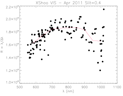
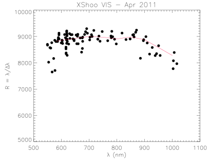
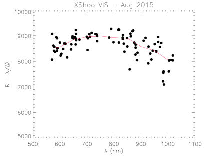
To measure the resolution of X-Shooter in the VIS arm, we reduced some calibration-lamp spectra following the same steps as for the science frames. We extracted the spectra from the pre-reduced images summing up the same columns of the detector where the stellar spectra fall in typical seeing conditions. We chose several tens of unblended emission lines that were fitted with Gaussians to obtain the line center $\lambda_{i}$ and the full width at half maximum (FWHM), $\Delta\lambda_{i}$ . The resolution $R_{i}=\lambda_{i}/\Delta\lambda_{i}$ is plotted as a function of wavelength in Fig. 18 for VIS spectra acquired with the 0 $\aas@@fstack{\prime\prime}$ 9 and 0 $\aas@@fstack{\prime\prime}$ 4 slits.

We note that the resolution with the 0 $\aas@@fstack{\prime\prime}$ 9 slit, $R\simeq 8800$ , is rather constant with $\lambda$ and decreases only slightly towards the edges of the spectrum. Moreover, it is basically unchanged between 2011 and 2015. For our analysis we adopted the value $R=8400$ , which is that of the region at $\lambda\simeq$ 9700 Å used for the $v\sin i$ determination.

The resolution with the 0 $\aas@@fstack{\prime\prime}$ 4 slit displays instead a higher variation with $\lambda$ ranging from $R\simeq 18\,500$ at the spectrum center to $R\simeq 16\,000$ near the edges. We adopted the value $R=17\,000$ in our analysis.

Appendix B Application of ROTFIT to the X-Shooter spectra

The template BT-Settl model spectra were first degraded in resolution to match that of the target spectrum and then resampled on its spectral points. Template and target spectra were then normalized to the local continuum or pseudo-continuum, paying attention to the spectral regions containing molecular bands, where the continuum level at wavelengths shorter than the band head was used as reference.

The code calculates the $\chi^{2}$ of the difference between observed and template spectra, where the rotational broadening was considered by convolving template spectra with a rotational profile²²2 The rotational broadening kernel (see, e.g., Gray 2005) assumes a linear limb-darkened star, with the limb-darkening coefficients from Claret et al. (2012). of increasing $v\sin i$ from 0 to 150 km s^-1 in steps of 1 km s^-1.

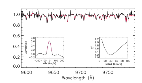
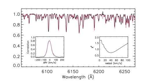
Table 4: Spectral regions analyzed with ROTFIT.

Range	Main features	$T_{\rm eff}$	$\log g$	$r$	$v\sin i$	RV
9590–9800	Ti i, Cr i	Y^a	N	Y	Y	Y
8160–8222	Na i	Y	Y	Y	N	Y
7600–7720	K i	Y	Y	Y	N	Y
7020–7120	TiO	Y	N	Y	N	Y
6050–6270	Ca i, Fe i, TiO	Y	Y	Y	Y^b	Y
5320–5500	Fe i	Y^b	Y^b	Y^b	N	N
5120–5220	Mg i b	Y^b	Y^b	Y^b	N	N
4400–4580	Fe i	Y^b	Y^b	Y^b	N	N

^a

Low sensitivity to this parameter.
^b

For the best exposed spectra of stars hotter than about 3500 K.

We selected a few spectral regions that are particularly suitable for the determination of one or more stellar parameters (Table 4). One of the main requirements is that these regions should be free, as much as possible, of strong emission lines produced by accretion or chromospheric activity. We mainly used the VIS spectra, but some portions of the UVB ones were used as well for the objects with spectra well exposed; these are mostly K-type stars and all earlier than M4. In each spectral interval, the sensitivity to a given parameter normally changes with the characteristics of the target and mainly depends on the SpT (i.e. $T_{\rm eff}$ ). Therefore, we have chosen spectral regions that are usable in the largest possible range of SpT.

B.1 $v\sin i$

The best intervals to perform an accurate determination of $v\sin i$ with ROTFIT are those devoid of very broad lines and strong molecular bands, but encompassing several strong absorption lines. A suitable region for the GK-type stars ranges from 6050 Å to 6270 Å, where some Ca i lines and a number of unblended lines, mostly of iron-group elements are present. These lines are also good diagnostics of temperature and gravity. However, a TiO molecular band starts to be visible for $T_{\rm eff}$ $\leq$ 4000 K and strongly affects the spectra of stars cooler than about 3500 K, for which reason we did not use that part of the spectrum for the determination of $v\sin i$ for cool objects, but it is still useful to measure $T_{\rm eff}$ in these cases. Another wavelength range suitable to measure $v\sin i$ with X-Shooter VIS spectra is between 9600 and 9800 Å³³3The final value of $v\sin i$ , which is reported in Table 1, is that one derived from the redder of the two spectral regions or the weighted average of the values derived in the two regions at 9700 Å and 6200 Å for the stars hotter than about 3500 K.. It includes several sharp absorption lines of Ti i and Cr i that are strong enough down to $T_{\rm eff}$ $\simeq$ 2900 K. Moreover, the intensity of these lines changes mildly with the SpT, thus they can also be used as temperature indicators, although their sensitivity to $T_{\rm eff}$ is not as high as that of other lines or molecular bands.

The results of the ROTFIT analysis for a rather rapid rotator (Sz 68) are illustrated in Fig. 19. The upper and lower panels show the observed spectrum around 9700 Å and 6150 Å, respectively. The best fitting template, i.e. the synthetic BT-Settl spectrum rotationally broadened, resampled and wavelength-shifted on the target spectrum that produces the minimum $\chi^{2}$ , is overplotted with a red dashed line in both panels. The CCF and the $\chi^{2}$ as a function of $v\sin i$ are also displayed in the insets.

B.2 $T_{\rm eff}$ and $\log g$

For the determination of the atmospheric parameters, the $v\sin i$ was kept fixed to the value derived through the analysis of the 9700-Å and 6150-Å spectral regions. To determine the gravity we selected two spectral regions containing the Na i doublet at $\lambda\approx 8190$ Å and the K i doublet at $\lambda\approx 7660-7700$ Å, whose wings are very sensitive to the electronic pressure and therefore to $\log g$ . In addition, we analyzed the spectral segment from 7020 to 7150 Å which contains three TiO molecular bands strongly sensitive to $T_{\rm eff}$ for cool stars and substellar objects.

Figure 20 displays an example of the results of the ROTFIT analysis for an M star (Sz 117). The left panels show the observed spectrum and the best fitting template, similarly to Fig. 19. The contour maps of the $\chi^{2}$ for each spectral region are shown in the right panels, where the 1 $\sigma$ confidence level is marked with a thick red line. For a better determination of the $T_{\rm eff}$ and $\log g$ values we have performed a quadratic interpolation onto a grid finer than the one of the models, with 10-K and 0.1-dex steps for $T_{\rm eff}$ and $\log g$ , respectively.

As mentioned above, for the hotter and best exposed sources we have also analyzed three spectral segments in the UVB spectra that cover the 5300–5500 Å, 5100–5250 Å, and 4400–4600 Å ranges. The spectral features they contain carry information about $T_{\rm eff}$ and $\log g$ and allow to evaluate the veiling at these shorter wavelengths. As an example, we show the fit of the UVB spectrum of Sz 68 (K2) in Fig 21. However, given the lower resolution of the UVB spectra, we did not use the latter to measure $v\sin i$ and RV.

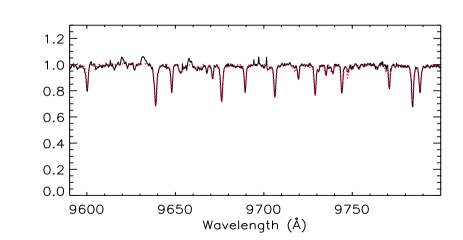
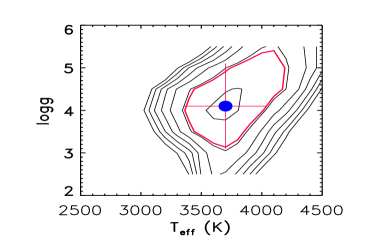
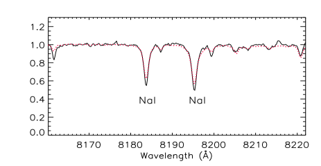
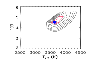
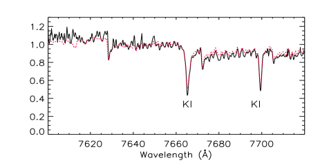
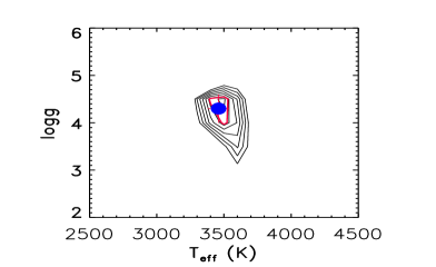
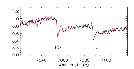
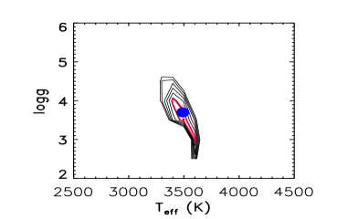
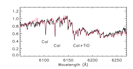
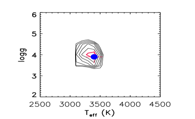
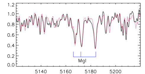
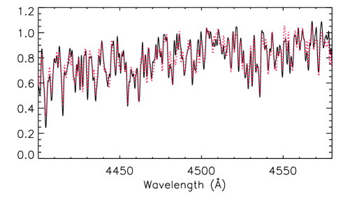
The adopted values of $\log g$ and $T_{\rm eff}$ are the weighted averages of the results for each spectral segment according to Table 4. These values are reported in Table 1 along with their errors and the veiling at five wavelengths.

For SSTc2dJ160034.4-422540 we failed to derive reliable atmospheric parameters because of the very low S/N of its spectrum. The VIS spectrum of this object does not display emission lines, which makes it unlikely to be a YSO. The reddest part of the VIS spectrum instead presents a number of molecular absorption bands which are indicative of a very low $T_{\rm eff}$ . We have thus performed a customized analysis of the whole spectral range from 8500 to 11 000 Å, which provided us with an estimate for $T_{\rm eff}$ and a value of RV. The spectral features present in this region do not provide solid constraints for $\log g$ , although this object has likely a low gravity. More details and a plot of its VIS spectrum can be found in Appendix D.

B.3 Veiling

The spectra of Class II sources, which typically undergo mass accretion from the circumstellar disk, can be affected by a different amount of veiling, which normally decreases at longer wavelengths, but it can still be noticeable in the IYJ bands (e.g., Fischer et al. 2011). For this reason, we also left the veiling free to vary. This was accomplished by adding to the templates, for each iteration, a wavelength-independent veiling in each spectral segment. This assumption is justified by the limited spectral ranges that we analyzed, which are, at most, 200 Å wide. Therefore, the “veiled” template is given by:

\biggl{(}\frac{F_{\lambda}}{F_{C}}\biggr{)}_{r}=\frac{\frac{F_{\lambda}}{F_{C}}+r}{1+r}\,,

(6)

where $F_{\lambda}$ and $F_{C}$ represent the line and continuum fluxes, respectively, and the veiling $r$ was let free to vary from 0.0 to 5.0 in 0.1 steps.

In cases of highly veiled spectra we often noticed the enhancement of $r$ with decreasing wavelength (see Fig. 22 for an example). This behavior is normally observed in strongly accreting objects (e.g., Hartigan et al. 1991; Fischer et al. 2011) and is interpreted as optically thick emission from the heated photosphere below the accretion shock (Calvet & Gullbring 1998). The decrease of the veiling at longer wavelengths is explained by the slow decline of the continuum accretion flux, which can be be approximated with a blackbody of $T\sim$ 10,000 K, and the steep rise of the photospheric flux from visible to near-IR wavelengths for late-type stars.

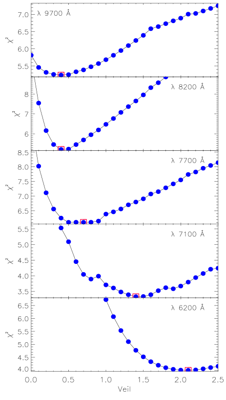
Appendix C Monte Carlo simulations for $v\sin i$

We run Monte Carlo simulation to evaluate the resolution in $v\sin i$ that can be reached with these data and our analysis code. To this aim, we built synthetic spectra at the same resolution and sampling as the X-Shooter ones. We broadened these spectra from 0 to 24 km s^-1 in steps of 1 or 2 km s^-1 and made 200 simulations per each $v\sin i$ , adding a random noise corresponding to signal-to-noise ratios S/N=20, 50, and 100. These simulations were made with BT-Settl spectra corresponding to $T_{\rm eff}$ = 2700, 3000, 3700, and 4800 K. We applied the code ROTFIT to each simulated spectrum, analogously to what we did with the target spectra, to determine the $v\sin i$ from the spectral region centered at 9700 Å. As apparent in Fig. 23, where only some examples are shown for the slit width 0 $\aas@@fstack{\prime\prime}$ 9 ( $R\simeq 8400$ ), we do not resolve $v\sin i$ values lower than 8 km s^-1. Thereafter, the measured $v\sin i$ starts to grow with the simulated $v\sin i$ and smoothly follows the one-to-one line. Therefore, we adopted 8 km s^-1 as upper limit in this configuration. The $v\sin i$ errors measured with ROTFIT on the target spectra were in most cases quite comparable with those inferred by the aforementioned Monte Carlo simulations, while for a few spectra they were larger. In these cases we have adopted the error of the simulation closest in $v\sin i$ , $T_{\rm eff}$ and S/N to the target spectrum.

We also made some tests for the high-resolution X-Shooter spectra (slit width 0 $\aas@@fstack{\prime\prime}$ 4, $R\simeq$ 17 000). In this case we obtained lower $v\sin i$ errors and we estimated an upper limit of 6 km s^-1 (Fig. 24).

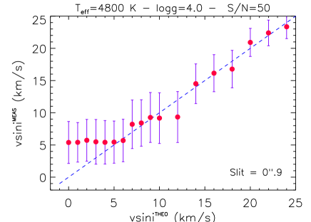
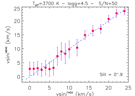
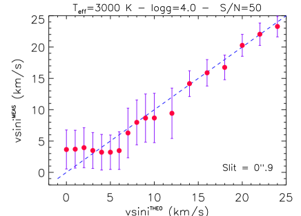
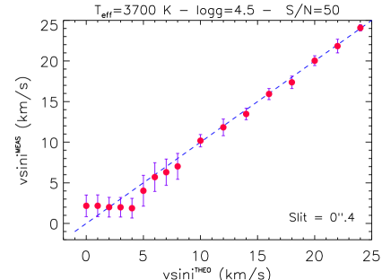
Appendix D Notes on individual objects

D.1 SSTc2d J160034.4-422540

SSTc2d J160034.4-422540 is a faint and very red (and/or reddened) source. The VIS spectrum does not show emission lines and has a very low signal in the spectral regions analyzed with ROTFIT, which makes the results of this code unreliable for this object. However, the reddest part of the VIS spectrum has a S/N sufficient to display the shape of the continuum and the molecular bands. We thus analyzed the flux-calibrated spectrum ranging from 8500 to 11 000 Å, with a method similar to the one adopted by Alcalá et al. (2006). In particular, we scaled to unity both the target and template spectra at 9170 Å, which is the wavelength of the head of a strong TiO molecular band. We artificially reddened the template spectra with the extinction law $A_{\lambda}/A_{V}$ of Cardelli et al. (1989), adopting the average interstellar value for total-to-selective extinction, $R_{V}=3.1$ . The extinction in the $V$ band, $A_{V}$ , was let free to vary. We kept the parameters of the model spectrum and the $A_{V}$ value that minimize the $\chi^{2}$ of the fit (see Fig. 25). As the shape of the TiO bands is not very sensitive to the gravity, $\log g$ is not well constrained by this fit, but, however, the atmospheric parameters found with this method ( $T_{\rm eff}$ =2000 K, $\log g$ =0) suggest a very cool giant star.

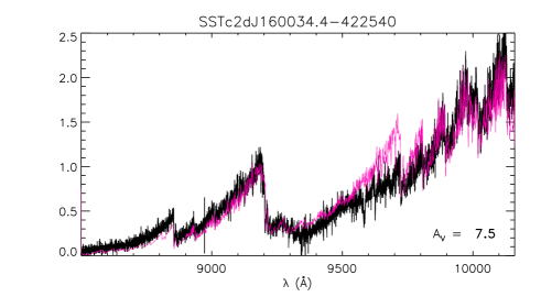
D.2 SSTc2d J160708.6-391408

This source is one of the brightest YSOs with a flat SED in Lupus (Merín et al. 2008; Evans et al. 2009). Its spectrum includes many permitted and forbidden emission lines, but the five VIS spectral segments listed in Table 4 are free from emission lines and have a S/N sufficient to be analyzed with ROTFIT.

We found $T_{\rm eff}$ = 3474 $\pm$ 206 K, which corresponds to an M2 spectral type according to the Pecaut & Mamajek (2013) calibrations. Alcalá et al. (2017) found a later spectral type (M5) but their results can also be consistent with an M3 type, the uncertainty resulting from the strong accretion and veiling of the spectrum. Our $T_{\rm eff}$ determination is more consistent with the M1.75 spectral classification of Muzic et al. (2014). We also estimated $T_{\rm eff}$ and extinction with the same method used for SSTc2dJ160034.4-422540. The results are shown in Fig. 26 where the observed spectrum is best fitted with a template with $T_{\rm eff}$ =3450 K and an extinction $A_{V}=3.5$ mag.

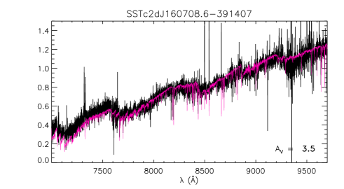
We dereddened the flux calibrated spectrum of SSTc2dJ160708.6-391408 (obtained merging the UVB, VIS, and NIR spectra) according to the Cardelli et al. (1989) law. Integrating the flux over all the X-Shooter wavelength range and multiplying for $2\pi d^{2}$ ( $d=200$ pc) we obtain a luminosity $L_{\star}$ $=0.032$ $L_{\odot}$ . However, it is difficult to distinguish the photospheric flux from that coming from the circumstellar matter in the SEDs of flat sources; therefore, the above measure must be considered as a rough estimate of the stellar luminosity. Nevertheless, this value makes the object rather subluminous in the HR diagram (green filled square in Fig. 6).

Since flat sources are believed to be YSOs still surrounded by an infalling envelope (Calvet et al. 1994), SSTc2d J160708.6-391408 may be in this evolutionary stage in which the energy output from the central star can heat the envelope. Therefore, the radiation emitted by the central object would be partly reprocessed by the envelope, i.e. it will emerge redistributed to longer wavelengths. In these conditions the bolometric luminosity of 0.18 $L_{\odot}$ , as derived by Evans et al. (2009), would be a better estimate of the total energy emitted by the central object. Adopting this value, SSTc2d J160708.6-391408 rises to the position marked by the arrowhead in Fig. 6, in good agreement with the other Lupus members. Moreover, as emphasized by Alcalá et al. (2017), the value of 0.18 $L_{\odot}$ would bring the ratio of accretion to bolometric luminosity in agreement with the YSOs of similar mass.

D.3 SSTc2dJ160708.6-394723 and SSTc2dJ161045.4-385455

The two non-members with Lithium, namely SSTc2dJ160708.6-394723 and SSTc2dJ161045.4-385455, are likely lithium-rich giants. The first star has $T_{\rm eff}$ $\simeq$ 4650 K and $\log g$ $\simeq$ 2.6 dex that locate it in the RGB region of the $\log g$ - $T_{\rm eff}$ diagram, close to the red clump locus (Fig. 4). For the second object we measured instead a larger gravity $\log g$ $\simeq$ 3.4 $\pm 0.9$ dex, which is more consistent with a subgiant or RG stage, taking into account the large error.

The origin of lithium-rich giants is still debated and different hypotheses have been put forward to explain the high lithium content in their atmospheres. The main scenarios that have been proposed are the regeneration of lithium in later evolutionary stages by the Cameron-Fowler mechanism (Cameron & Fowler 1971), the engulfment of Li-rich substellar companions (e.g., Alcalá et al. 2011b; Casey et al. 2016, and references therein) or inhibition of mixing because of fossil magnetic fields of their Ap-type progenitors (e.g., Smiljanic et al. 2016).