SCYNet: Testing supersymmetric models at the LHC with neural networks

Abstract

SCYNet (SUSY Calculating Yield Net) is a tool for testing supersymmetric models against LHC data. It uses neural network regression for a fast evaluation of the profile likelihood ratio. Two neural network approaches have been developed: one network has been trained using the parameters of the 11-dimensional phenomenological Minimal Supersymmetric Standard Model (pMSSM-11) as an input and evaluates the corresponding profile likelihood ratio within milliseconds. It can thus be used in global pMSSM-11 fits without time penalty. In the second approach, the neural network has been trained using model-independent signature-related objects, such as energies and particle multiplicities, which were estimated from the parameters of a given new physics model. While the calculation of the energies and particle multiplicities takes up computation time, the corresponding neural network is more general and can be used to predict the LHC profile likelihood ratio for a wider class of new physics models.

1 Introduction

Direct searches for new particles at the LHC are among the most sensitive probes of beyond the Standard Model (BSM) physics and play a crucial role in global BSM fits. Calculating the profile likelihood ratio (referred to as $\chi^{2}$ in the following) for a new physics model from LHC searches is straightforward in principle: for each point in the model parameter space, signal events are generated using a Monte-Carlo simulation. The $\chi^{2}$ is then calculated from the number of expected signal events, the Standard Model background estimate and the number of observed events for a given experimental signal region. The computation time for such simulations, can be overwhelming however, especially when testing BSM scenarios with many model parameters. Global fits of supersymmetric (SUSY) models, for example, are typically based on the evaluation of ${\cal O}(10^{9})$ parameter points, see e.g. killingcmssm ; deVries:2015hva ; Strege:2014ija , and the required Monte-Carlo statistics for estimating the number of signal events for each parameter point requires up to several hours of CPU time. In this study we have attempted to provide a fast evaluation of the LHC $\chi^{2}$ for generic SUSY models by utilizing neural network regression.

Global SUSY analyses which combine low-energy precision observables, like the anomalous magnetic moment of the muon, and LHC searches for new particles strongly disfavour minimal SUSY models, like the constrained Minimal Supersymmetric Standard Model (cMSSM) killingcmssm . Thus, more general supersymmetric models have to be explored, including for example the phenomenological MSSM (pMSSM-11) Djouadi:1998di , specified by eleven SUSY parameters defined at the electroweak scale. The pMSSM-11 allows to accommodate the anomalous magnetic moment of the muon, the dark matter relic density and the LHC limits from direct searches. However, the large number of model parameters poses a significant challenge for global pMSSM-11 fits.

(a) Direct approach

(b) Reparametrized approach

Figure 1: Flowchart indicating how we have calculated the LHC $\chi^{2}$ via the direct (a) and reparametrized (b) neural network regression approach described in the text. Throughout the paper, the subscript “SN” denotes the $\chi^{2}$ obtained via SCYNet.

In this paper we introduce the SCYNet tool for the accurate and fast statistical evaluation of LHC search limits – and potential signals – within the pMSSM-11 and other SUSY models. SCYNet is based on the results of a simulation of new physics models that used CheckMATE 2.0 Drees:2013wra ; Kim:2015wza ; Dercks:2016npn , and the subsequently calculated $\chi^{2}$ from event counts in the signal regions of a large number of LHC searches. The $\chi^{2}$-estimate has been used as an input to train a neural network based regression; the resulting neural network then provides a very fast and reliable evaluation of the LHC search results, which can be used as an input to global fits.

Neural networks allow predictions of complex data by overlapping non-linear functions in an efficient manner, and are straightforward to implement using open source libraries like Tensorflow tensorflow2015-whitepaper , Theano theano and Keras keras . Previous studies Buckley:2011kc ; Bornhauser:2013aya ; Caron:2016hib have used neural networks (and other machine learning techniques) mainly as a classifier between allowed and excluded models. Going beyond this simple classification, recently Gaussian processes Rasmussen2004 were used to predict the number of signal events for a simple SUSY model Bertone:2016mdy . Here, we have applied neural networks as a regression tool to predict $\chi^{2}$ values for an ensemble of many signal regions. Compared to other regression methods, neural networks excel when dealing with sparse sample sets due to their non-linear nature. They can thus be valuable tools for predicting LHC $\chi^{2}$ values of complex BSM models.

In order to train and validate the neural network regression we have considered the pMSSM-11 as an example of a complex and phenomenologically highly relevant SUSY model. Two different approaches have been explored: in the so-called direct approach we have simply used the eleven parameters of the pMSSM-11 as input to the regression, c.f. Figure 1a. The resulting neural network evaluates the $\chi^{2}$ of the pMSSM-11 within milliseconds and can thus be used in global pMSSM-11 fits without time penalty. A second, so-called reparametrized, approach uses SUSY particle masses, cross sections and branching ratios to first estimate signature-based objects, such as particle energies and particle multiplicities, which should relate more closely to the LHC $\chi^{2}$ values (Figure 1b). While the calculation of the particle energies and multiplicities requires extra computation time, the corresponding neural network should be more general and be able to predict the $\chi^{2}$ for a wider class of SUSY models. To explore this feature, we have examined how well a reparametrized neural network trained on the pMSSM-11 can predict the $\chi^{2}$ for two other popular SUSY models, namely the cMSSM and a model with anomaly mediated SUSY breaking (AMSB) Randall:1998uk ; Giudice:1998xp .

This paper is structured as follows: In section 2 we provide details of the LHC event generation within the pMSSM-11, and the method we have used to calculate a global LHC $\chi^{2}$. The training and validation of the direct and reparametrized neural net approaches are presented in 3 and 4, respectively. The results are summarized and our conclusions presented in section 5. More details on the statistical approach are given in the appendices.

2 Event generation and LHC $\chi^{2}$ calculation

For the training and testing of the neural networks we have calculated the LHC $\chi^{2}$ for a set of pMSSM-11 parameter points using CheckMATE. This $\chi^{2}_{\rm CM}$ calculation (the subscript “CM” denotes the CheckMATE result) required the generation of SUSY signal events, a detector simulation and the evaluation of the LHC analyses. In this section we describe the simulation chain, list the LHC analyses we include, and explain our calculation of $\chi^{2}_{\rm CM}$ from the event counts in the various experimental signal regions. A graphical depiction of this process can be found in Figure 2.

Figure 2: Flow chart of the simulation chain we have used in the sample generation. The subscript “CM” in $\chi^{2}_{\rm CM}$ denotes $\chi^{2}$-values obtained using CheckMATE.

pMSSM-11 Parameter	Description	Range
$M_{1}$	Bino mass	[-4000,4000] GeV
$M_{2}$	Wino mass	[100,4000] GeV
$M_{3}$	Gluino Mass	[-4000,-400]$\cup$[400,4000] GeV
$M(\tilde{Q}_{12})$	1st and 2nd gen. scalar squark mass	[300,5000] GeV
$M(\tilde{Q}_{3})$	3rd gen. scalar squark mass	[100,5000] GeV
$M(\tilde{L}_{12})$	1st and 2nd gen. scalar slepton mass	[100,3000] GeV
$M(\tilde{L}_{3})$	3rd gen. scalar slepton mass	[100,4000] GeV
$M(A)$	Pseudoscalar Higgs pole mass	[0,4000] GeV
$A$	Third generation trilinear coupling	[-5000,5000] GeV
$\mu$	Higgsino mass parameter	[-5000,-100]$\cup$[100,5000] GeV
$\tan(\beta)$	Higgs doublet vacuum expectation value	[1,60] GeV

Table 1: pMSSM-11 ranges we have used for the sample generation. The lower bounds on the mass parameters were motivated by the current collider bounds for SUSY particle production. The relatively large range for third generation trilinear coupling $A$ were motivated by the observed Higgs mass. All the pMSSM-11 parameters were defined at a scale of 1 TeV AguilarSaavedra:2005pw .

The pMSSM-11 is based on eleven SUSY parameters: the bino, wino and gluino mass parameters, $M_{1},M_{2},M_{3}$, the scalar quark and lepton masses of the 1st/2nd and 3rd generation, respectively, $M(\tilde{Q}_{12})$, $M(\tilde{Q}_{3})$, $M(\tilde{L}_{12})$, $M(\tilde{L}_{3})$, the mass of the pseudoscalar Higgs, $M(A)$, the trilinear coupling of the 3rd generation, $A$, the Higgsino mass parameter, $\mu$, and the ratio of the two vacuum expectation values, $\tan(\beta)$ Djouadi:1998di . The ranges of the pMSSM-11 parameters we have considered are specified in Table 1.

We have sampled pMSSM-11 points using both a uniform and a Gaussian random probability distribution. The maximum and standard deviation of the Gaussian distribution have been chosen to be one fourth and one half of the parameter range, respectively. Consequently we have generated less points near the edges of the parameter range, and in the decoupling regime of large pMSSM-11 parameters, where the SUSY spectra are beyond the LHC reach.

After we have generated a pMSSM-11 parameter point we have used SPheno-3.3.8 spheno to calculate the spectrum. Following the SPA convention AguilarSaavedra:2005pw , all 11 parameters were defined at a scale of 1 TeV. We have then only proceeded in the simulation chain if the following preselection criteria have been fulfilled:

• There were no tachyons in the spectrum.

• The $\chi^{0}_{1}$ was the LSP, such that it was the dark matter candidate.

• Both Higgs bosons ($h^{0}$, $H^{0}$) had a mass above 110 GeV.

• $m_{\chi_{1}^{\pm}}>$103.5 GeV Agashe:2014kda

• The experimental value and the predicted value for the electroweak precision observables $m_{W},~{}|\Delta(M_{Bs}),~{}\mbox{BR}(B_{s}\rightarrow\mu\mu),~{}\mbox{BR}(b\rightarrow s\gamma),~{}\mbox{BR}(B_{u}\rightarrow\tau\nu)$ differed by less than 5 times the total uncertainty given in Table 2.

The preselection criteria were applied in order to restrict the SUSY parameter space to phenomenologically viable regions. Consequently, the neural networks that were trained on that parameter space will only be valid if the preselection criteria are fulfilled. Note that the anomalous magnetic moment of the muon, $(g-2)_{\mu}$, has not been included in the preselection criteria, because in a global fit one might not wish to include this observable.

Precision observable	Experimental value	Theoretical uncertainty	Ref.
$m_{W}$	$(80385\pm 15)\mbox{MeV}$	0.1%	Group:2012gb
BR(b $\rightarrow$ s $\gamma$)	$(3.43\pm 0.21\pm 0.07)\cdot 10^{-4}$	14 %	Amhis:2012bh
BR($B_{s}$ $\rightarrow$ $\mu^{+}$ $\mu^{-}$)	$(2.9\pm 0.7)\cdot 10^{-9}$	26 %	CMSandLHCbCollaborations:2013pla
BR($B_{u}$ $\rightarrow$ $\tau$ $\nu$)	$(1.05\pm 0.25)\cdot 10^{-4}$	20 %	Beringer:1900zz
$|\Delta(M_{Bs})|$	$(17.719\pm 0.036\pm 0.023)\ \mbox{ps}^{-1}$	24 %	Beringer:1900zz

Table 2: Precision observables used to constrain the parameter space. Note that a newer and slightly more precise measurement BR($B_{s}$ $\rightarrow$ $\mu^{+}$ $\mu^{-})=(2.8^{+0.7}_{-0.6})\cdot 10^{-9}$ is now available but was not included in the preselection CMS:2014xfa .

Nr.	Name	Description	$\mathcal{L}[$fb${}^{-1}]$	$N_{\rm SR}$	Ref.
Analyses @ 8 TeV
1	atlas_1402_7029	3 leptons + $\not{E}_{T}$	20.3	24	ATLAS-1402-7029
2	atlas_1403_5294	2 leptons + $\not{E}_{T}$	20.3	9	ATLAS-1403-5294
3	atlas_conf_2013_036	4 or more leptons	20.7	5	ATLAS-CONF-2013-036
4	atlas_1308_2631	2 b-jets + $\not{E}_{T}$	20.1	6	ATLAS-1308-2631
5	atlas_1403_4853	2 leptons(opposite sign)	20.3	12	ATLAS-1403-4853
6	atlas_1404_2500	2 leptons(same sign) + jets	20.3	5	ATLAS-1404-2500
7	atlas_1405_7875	Multiple jets + $\not{E}_{T}$	20.3	15	ATLAS-1405-7875
8	atlas_1407_0583	1 isolated lepton + jets + $\not{E}_{T}$	20.3	27	ATLAS-1407-0583
9	atlas_1407_0608	2 stop quarks	20.3	3	ATLAS-1407-0608
10	atlas_1502_01518	1 jet + $\not{E}_{T}$	20.3	9	ATLAS-1502-01518
11	atlas_1503_03290	2 leptons(same flavor, opposite sign) + $\not{E}_{T}$	20.3	1	ATLAS-1503-03290
Analyses @ 13 TeV
12	atlas_conf_2015_076	1 isolated lepton + jets + $\not{E}_{T}$	13.3	6	ATLAS-CONF-2015-076
13	atlas_1602_09058	Jets + 2 leptons(same sign) or 3 leptons	3.2	4	ATLAS-1602-09058
14	atlas_1605_03814	Multiple jets + $\not{E}_{T}$	3.2	7	ATLAS-1605-03814
15	atlas_conf_2015_082	Leptonically decaying Z + jets + $\not{E}_{T}$	3.2	1	ATLAS-CONF-2015-082
16	atlas_1604_07773	1 jet + $\not{E}_{T}$	3.2	13	ATLAS-1604-07773
17	atlas_conf_2016_013	Multiple leptons + Multiple Jets	3.2	10	ATLAS-CONF-2016-013
18	atlas_conf_2015_067	b-jets + $\not{E}_{T}$	3.2	3	ATLAS-CONF-2015-067
19	cms_pas_sus_15_011	2 leptons(same flavor, opposite sign) + $\not{E}_{T}$	2.2	47	CMS-PAS-SUS-15-011

Table 3: Analyses considered at 8 TeV and 13 TeV. The names correspond to the internal CheckMATE nomenclature. $\mathcal{L}$ denotes the luminosity and $N_{\rm SR}$ the number of SRs for each analysis.

2.1 Event generation

If all pre-selection criteria were fulfilled we then generated LHC signal events for 8 and 13 TeV. At 8 TeV we simulated the production of both electroweak and strongly interacting SUSY particles, including all possible $2\to 2$ scattering processes. The 8 TeV analyses were included since no 13 TeV electroweak searches were available at the time the event generation for this work was started. For the simulation of the electroweak events, which include all combinations of slepton, chargino and neutralino final states, we used MadGraph5_aMC@NLO 2.4 madgraph with the CTEQ6L1 PDF Nadolsky:2008zw and showered the events with Pythia 6.428 pythia6_4_manual . Since the LHC is only sensitive to electroweak production if $m_{\chi^{0}_{1}}<500$ GeV sensitivity_8TeV_ATLAS_EW , we have only simulated the electroweak processes if this was the case. The processes which contain final states with strongly interacting SUSY particles, i.e. squarks and gluinos, were simulated using Pythia 8.2 pythia8 ; Desai:2011su , with cross sections normalized to NLO using NLL-Fast 2.1 nll_fast_1 ; nll_fast_2 ; nll_fast_3 ; nll_fast_4 ; nll_fast_5 ; nll_fast_6 ; nll_fast_7 ; nll_fast_8 .

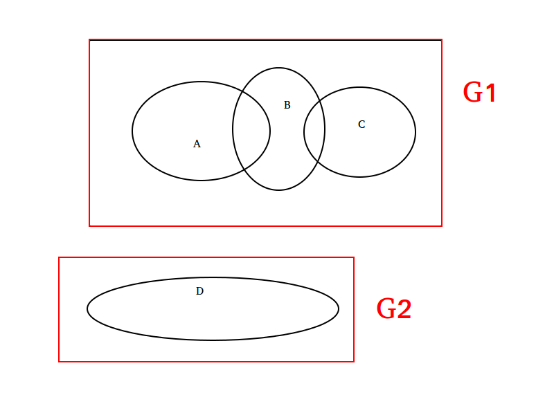
Figure 3: Example for a disjoint group selection for one analysis. The analysis has four SRs (A,B,C,D). Because SR A overlaps with SR B and SR B overlaps with SR C, we grouped SR A,B and C into one disjoint group G1. Because SR D does not overlap with any of the other SR of the analysis, the disjoint group G2 only contains the SR D.

At 13 TeV, only processes with strongly interacting SUSY particles were simulated, since all analyses which were available within CheckMATE target these final states. We have again used MadGraph5_aMC@NLO 5.2.4 madgraph to generate events and Pythia 6.248 pythia6_4_manual was used to decay and shower the final state. The cross sections were normalized to NLO accuracy as obtained from NLL-Fast 2.1 nll_fast_1 ; nll_fast_2 ; nll_fast_3 ; nll_fast_4 ; nll_fast_5 ; nll_fast_6 ; nll_fast_7 ; nll_fast_8 . One additional parton was generated at the matrix element level and then matched to the parton shower if the mass gap between either the lightest squark or the gluino and the LSP was below 300 GeV. Such a procedure allowed for the accurate determination of the signal acceptance in compressed spectra where initial state radiation is crucial to pass the experimental cuts Dreiner:2012gx ; Dreiner:2012sh .

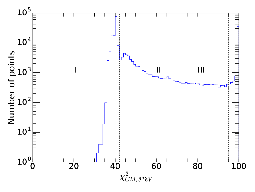
(a)

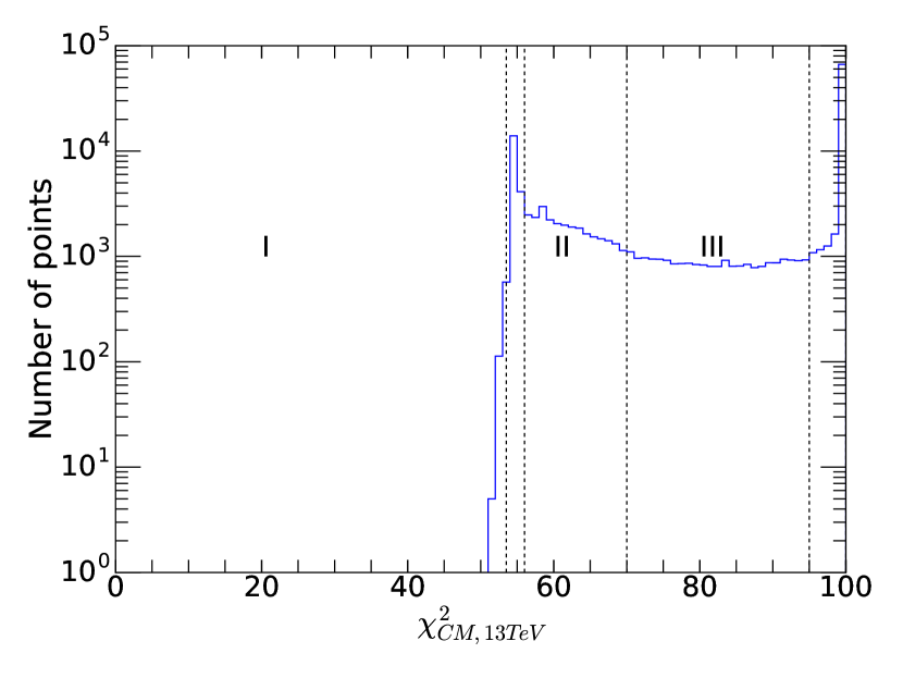
(b)

Figure 4: Distributions of $\chi^{2}_{\rm CM}$ for 8 TeV (a) and 13 TeV (b). The dashed lines indicate ranges for which we evaluated the performance of the SCYNet neural network separately as described in the text.

For 8 TeV we calculated $\chi^{2}_{\rm CM}$ for a total of 210000 pMSSM-11 parameter points and at 13 TeV we simulated 140000 parameter points. To guarantee a sufficient statistical accuracy, we have generated between 1000 and 45000 events per particle production process, depending in detail on the expected number of signal events. For each pMSSM-11 parameter point we have simulated on average 20000 events, which required approximately 380000 CPU hours in total.

Once the event generation was completed, the event files were passed through CheckMATE Drees:2013wra ; Kim:2015wza ; Dercks:2016npn which contains a tuned Delphes-3 delphes detector simulation with separate setups for 8 and 13 TeV. The analyses which have been used to train the SCYNet neural network regression are listed in Table 3.

2.2 LHC $\chi^{2}$ calculation with CheckMATE

We have implemented a calculation of $\chi^{2}_{\rm CM}$ that approximates to a likelihood, based on the CheckMATE output of the event count in each signal region (SR). In the following we will use $\chi^{2}_{{\rm CM},jk}$ to denote the $\chi^{2}$ of analysis $j$ and SR $k$ from CheckMATE. The exact statistical prescription we have used to calculate $\chi^{2}_{{\rm CM},jk}$ for each single SR is described in A.

The individual signal regions were combined to give a global $\chi^{2}_{\rm CM}$ with a procedure that combined the most sensitive (expected) orthogonal SRs. Our algorithm chose these by first dividing the SRs in each analysis into orthogonal disjoint groups. Each disjoint group can contain several SRs and the SRs of one disjoint group are disjoint to all SRs in all other disjoint groups, see Figure 3. If one disjoint group contains more than one SR, the SR with the largest $\mbox{signal}/S^{95}_{\mbox{exp}}$ ratio in this group was selected. For one analysis we then added the $\chi^{2}$s of all selected SRs, $\chi^{2}_{{\rm CM},j}:=\sum\limits_{\mathclap{{\rm selected}\;k}}\ \chi^{2}_{{\rm CM},jk}$. In the last step all the $\chi^{2}_{{\rm CM},j}$ from the individual analyses have been added to give the overall $\chi^{2}_{\rm CM}:=\sum\limits_{j}\chi^{2}_{j}$. All the analyses we have combined for the same centre-of-mass energy target different final state topologies, and we have therefore assumed that the SRs of different analyses were to a very good approximation disjoint. In the case of the 8 (13) TeV analyses we found 47 (65) disjoint SRs for the group with the largest sensitivity.

Since the experimental collaborations do not provide information on the correlation of the systematic errors, we had to assume the uncertainties were Gaussian distributed and uncorrelated.

Figures 4(a) and 4(b) show the distributions of $\chi^{2}_{\rm CM}$ for all sampled points. Two peaks can be observed in both plots: the first peak, called the zero signal peak, is located at around $\chi^{2}_{\rm CM}\approx 40$ (8 TeV, left plot) and $\chi^{2}_{\rm CM}\approx 54$ (13 TeV, right plot), respectively. All $\chi^{2}_{\rm CM}$ values in the zero signal peaks belong to pMSSM-11 parameter points with very heavy SUSY spectra and thus very little or no expected signal in any of the SRs. A second peak occurs at $\chi^{2}=100$ because we set all $\chi^{2}_{\rm CM}>100$ to this value. This was done to avoid the neural networks learning any structures at large $\chi^{2}_{\rm CM}>100$, where the model is already clearly excluded by the LHC data.

The three regions labeled I, II and III outside of the zero signal peak and the peak at $\chi^{2}_{\rm CM}=100$ in Figures 4(a) and 4(b) are called rare target ranges. We differentiated between regions below (I) and above (II and III) the zero signal peak and between regions with $\chi^{2}_{\rm CM}$ closer to the minimum (I and II), since these are much more important for global fits than those far away, and thus need better modeling. We have evaluated the performance of the SCYNet neural network separately for these different regions.

3 Neural network regression: direct approach

In this section the direct approach for neural network regression used in SCYNet has been described. The inputs to the network were the 11 parameters of the pMSSM-11 and the output, $\chi^{2}_{\rm SN}$, is an estimate of $\chi^{2}_{\rm CM}$ for the LHC searches described in section 2. We have trained separate networks for the 8 and 13 TeV analyses, with outputs $\chi^{2}_{\rm SN,8\,TeV}$ and $\chi^{2}_{\rm SN,13\,TeV}$, respectively. In this section, the setup and performance of both networks has been discussed, but we have focused on the results obtained for $\chi^{2}_{\rm SN,8\,TeV}$ for illustration.

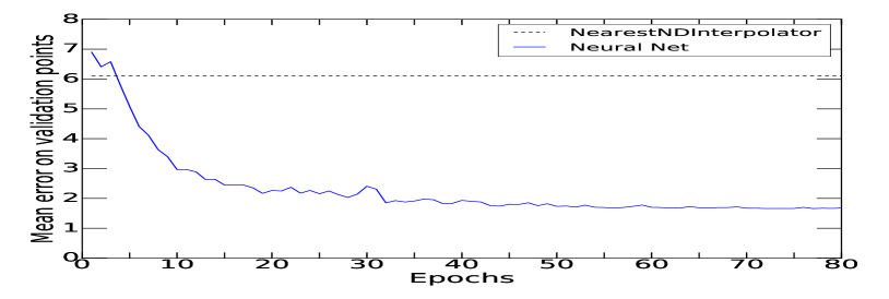
(a)

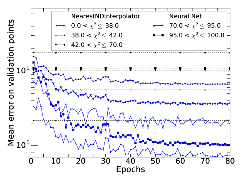
(b)

Figure 5: Evolution of the mean error on points in the validation set during training on the 8 TeV LHC $\chi^{2}_{\rm CM}$ compared to a nearest neighbour interpolator for all points (a), divided into different $\chi^{2}_{\rm CM}$ ranges (b).

3.1 Parameters of the neural networks

All neural networks used in this work were of the simple feed forward type and have been designed using the Tensorflow tensorflow2015-whitepaper library. We performed scans of the neural network parameters (so-called hyperparameters) to find the best configuration. The hyperparameters, which we were trying to optimize, were the number of hidden layers, the number of neurons in the hidden layers, the dropout probability of neurons in the hidden layers, the batch size, the learning rate of the Adam minimization algorithm adam_optimizer , the activation function in the output neuron, the regularization parameter and the type of cost function. The networks discussed in this section always refer to the hyperparameter configuration that was found to function best.

Our 8 TeV network had four hidden layers $l=1,\ldots,4$, each with $N_{l}=300$ neurons and all neurons have hyperbolic tangent activation functions. The weights in layer $l$ were initialized with a Gaussian distribution with standard deviation $1/\sqrt{N_{l-1}}$ and mean zero, while the biases were initialized with a Gaussian distribution with standard deviation equal to one and mean equal to zero. In order to train a network with a hyperbolic tangent output activation function, the targets were transformed to the range between $-1$ and $1$ with a modified Z-score normalization (see details in B).

8 TeV
$\chi^{2}$ range	$0-38$	$38-42$	$42-70$	$70-95$	$95-100$
Direct	1.9	0.7	3.7	6.7	1.0
Reparameterized	1.6	0.5	3.6	7.3	1.0
13 TeV
$\chi^{2}$ range	$0-53.5$	$53.5-56$	$56-70$	$70-95$	$95-100$
Direct	1.8	0.9	2.4	4.0	0.5
Reparameterized	2.0	0.7	2.2	4.7	0.3

Table 4: Mean errors of the neural networks for the 8 TeV and 13 TeV LHC $\chi^{2}$ prediction in different ranges. The results for the direct and reparameterized approach (section 4) are compared.

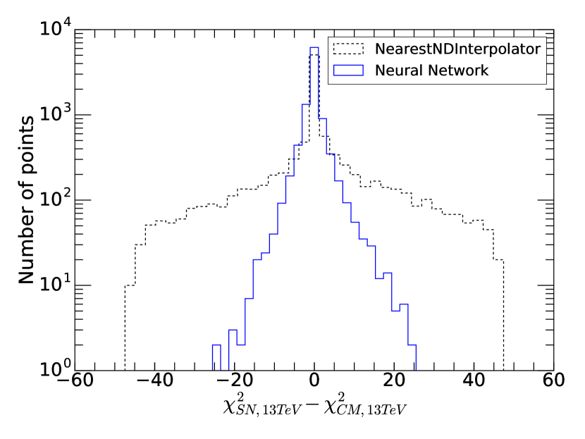
(a)

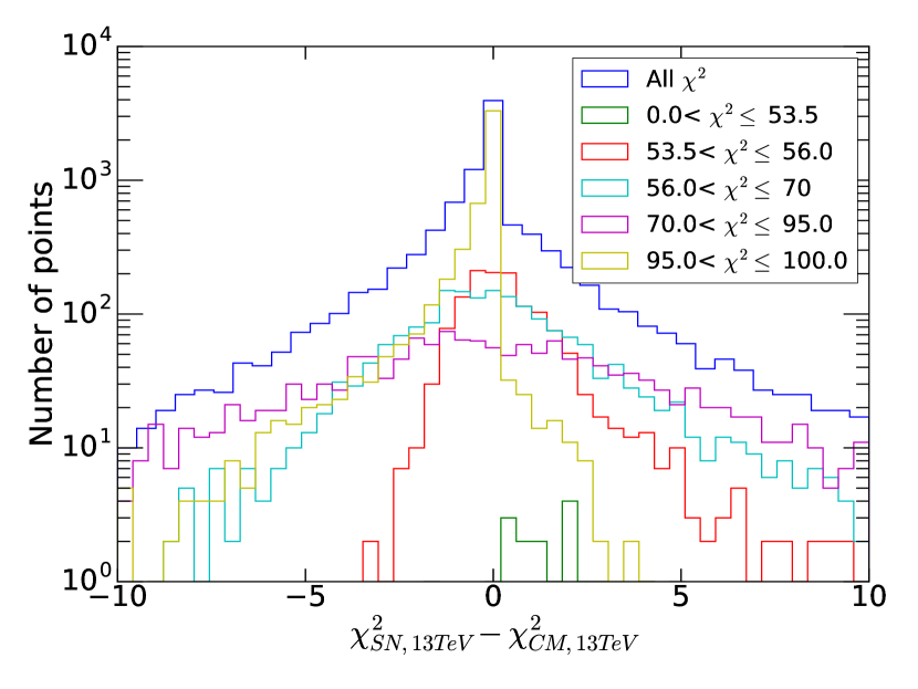
(b)

Figure 6: Error histogram for the neural network compared to the nearest neighbor interpolator for all validation points (a), divided by $\chi^{2}$ ranges (b).

During the training we used a quadratic cost function and trained with a batch size of 750. We used the Adam minimization algorithm with a learning rate of 0.001 and all other parameters of the Adam optimizer were set to the default values from adam_optimizer .

The complete cost function $C$ consists of the quadratic cost function and a quadratic regularization:

$$C=\mbox{quadratic cost}+\frac{\lambda}{2N_{{\rm train}}}\sum\limits_{jkl}(w_{jk}^{l})^{2},$$ (1)

where $N_{{\rm train}}$ were the number of points in the training set. We used 10000 validation points ($N_{{\rm val}}=10000$) while the rest of the sampled points were used for training. In the hyperparameter scan we found that $\lambda=10^{-5}$ gave the best network performance.

The 13 TeV network had the same structure as the 8 TeV network but the batch size during training was slightly adjusted to 500, while all other hyperparameters were the same as in the 8 TeV case.

3.2 Training the neural networks

The training phase of the 8 TeV neural network has been visualized in Figures 5(a) and 5(b) where we have compared the mean error on points in the validation data during the training phase to that of a nearest neighbor interpolator. The following parameter has been used to quantify the network performance,

$$\mbox{Mean error on valid. points}:=\frac{1}{N_{{\rm val}}}\sum\limits_{i=1}^{N_{{\rm val}}}|\chi^{2}_{{\rm CM}_{i}}-\chi^{2}_{{\rm SN}_{i}}|.$$ (2)

After the last training epoch the mean error on points in the validation set is 1.68. As shown in Figure 5(a) this performance is a significant improvement over a nearest neighbor interpolator scipy .

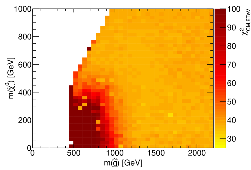
(a)

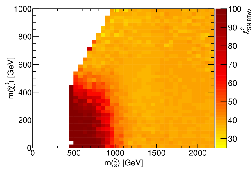
(b)

Figure 7: Minimum pMSSM-11 $\chi^{2}$ in the gluino-neutralino mass plane for the 8 TeV validation set for the CheckMATE results (a) and the predictions of SCYNet (b).

Figure 5(b) shows how the mean errors for $\chi^{2}$ values in the different ranges defined in Figures 4(a) and 4(b) behaved during the training phase. The corresponding mean errors after the last training epoch can be found in Table 4. The mean errors in the rare target ranges I ($0<\chi^{2}\leq 38$), II ($42<\chi^{2}\leq 70$), and III ($70<\chi^{2}\leq 95$) were larger than the mean errors in the zero signal range and in the range around 100. This behaviour will be called rare target learning problem (RTLP) in the following and can be understood from the $\chi^{2}_{\rm CM}$ distribution in Figure 4(a) and the corresponding discussion in section 2.2: the majority of the scanned pMSSM-11 points led to $\chi^{2}_{\rm CM}$ values in the range $38<\chi^{2}\leq 42$ and $95<\chi^{2}$, which were thus described more accurately by the neural network than those in regions I, II and III.

In future work the RTLP will be addressed with two strategies: the 11-dimensional probability density function (pdf) in the parameter space of the points in the range $0<\chi^{2}\leq 38$ and $42<\chi^{2}\leq 95$ will be used to randomly sample new pMSSM-11 points which will be added to the training and validation samples. In the second approach, each point in the RTLP region will be used to seed new random points using a narrow 11-dimensional pdf centered around each point in the above-mentioned $\chi^{2}$ range. New points can then be generated, simulated and used to improve the network especially in the rare target ranges. Motivated by the profile likelihood requirement, which sets an estimate of $\Delta\chi^{2}=1$ for the $1\,\sigma$ range, we plan to improve the training and validation set size by subsequent application of these procedures until a mean error of $\Delta\chi^{2}$ well under 1 is reached.

For the 13 TeV neural network we found similar results to those from the 8 TeV network that has already been displayed in Figure 5(a) and 5(b). The mean errors for the 13 TeV network at the end of the training phase have been given in Table 4. The histogram in Figure 6(a) shows the difference between the CheckMATE and SCYNet results $\chi^{2}_{\rm SN}-\chi^{2}_{\rm CM}$. Again the comparison to the nearest neighbour interpolator shows that the neural network provides a much more powerful tool to predict the LHC $\chi^{2}$. The mean error for the neural network on points in the validation set is 1.45.

The performance of the 13 TeV network is also different for the different $\chi^{2}$ ranges, see Figure 6(b). However, the difference between the mean error in the zero signal range and in the rare target ranges is less pronounced than for the 8 TeV network. This can be understood from comparing Figures 4(a) and 4(b): the 13 TeV LHC analyses are sensitive to a wider range of pMSSM-11 parameters, and thus fewer of the sampled points result in no signal expectation.

(a)

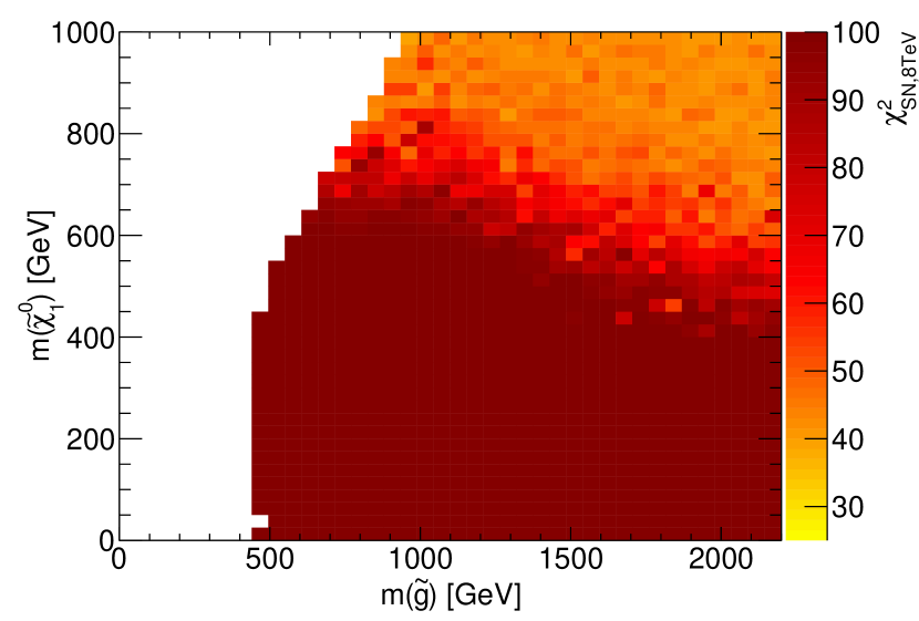
(b)

Figure 8: Maximum pMSSM-11 $\chi^{2}$ in the gluino-neutralino mass plane for the 8 TeV validation set for the CheckMATE results (a) and the predictions of SCYNet (b).

3.3 Testing the neural networks

In this section we have used an additional, statistically independent validation set of 60000 pMSSM-11 points that passed the preselection criteria to compare the SCYNet prediction to the CheckMATE result. For illustration we have focused on the projection of the 11-dimensional pMSSM parameter space onto the masses of the gluino $\tilde{g}$ and the neutralino $\chi^{0}_{1}$, which are particularly relevant for the $\chi^{2}$ of the LHC searches. All plots in this section have been given for the 8 TeV case, while similar results were obtained for the 13 TeV case.

In Figure 7(a) we have presented the minimal $\chi^{2}_{\rm CM}$ obtained by CheckMATE for the validation set of pMSSM-11 points in bins of the gluino and neutralino masses. The minimum $\chi^{2}$ in each ($m(\tilde{g}),m(\tilde{\chi}^{0}_{1})$)-bin typically corresponds to scenarios, where all other SUSY particles, and in particular squarks of the first two generations, were heavy and essentially decoupled from the LHC phenomenology.

In Figure 7(b) the corresponding result obtained from the SCYNet neural network regression has been given. We found that the neural network reproduces the main features of the $\chi^{2}$ distribution. We emphasize here that each bin represents a single pMSSM-11 parameter point and consequently the results show that the network successfully reproduces the LHC results across the whole plane.

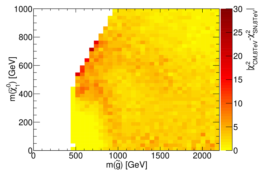
Figure 9: Difference between the CheckMATE and SCYNet $\chi^{2}$predictions in the gluino-neutralino mass plane for all 8 TeV validation points. In each bin the mean difference has been calculated for all validation points.

Figures 8(a) and 8(b) again show the $\chi^{2}_{\rm CM}$ and $\chi^{2}_{\rm SN}$ values as a function of the gluino and neutralino masses, but now have we displayed the maximum $\chi^{2}$ in each bin. Comparing the two figures proves that the neural network reproduces the main features of the $\chi^{2}$ distribution well.

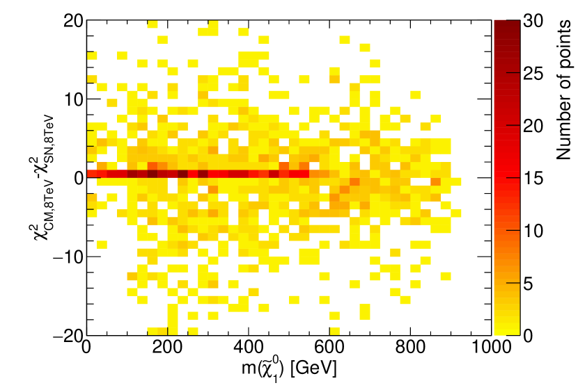
(a)

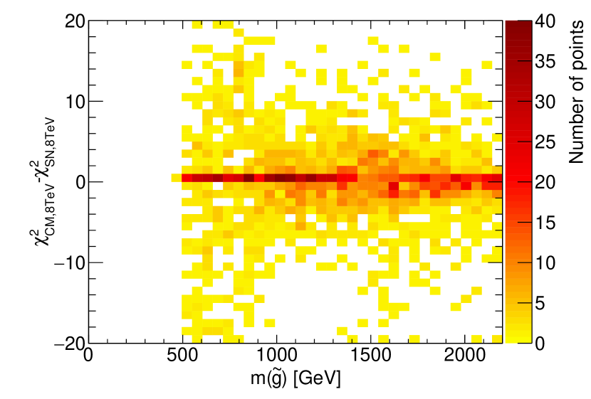
(b)

Figure 10: Using all validation points from figure 9, we show the difference between the SCYNet parametrization and the CheckMATE result against $m(\tilde{\chi}^{0}_{1})$ for gluino masses between 850 and 900 GeV (b) and against $m(\tilde{g})$ for neutralino masses between 400 and 450 GeV (b).

The difference between the CheckMATE and SCYNet result, $\chi^{2}_{\rm CM,8\,TeV}-\chi^{2}_{\rm SN,8\,TeV}$ has been presented in Figure 9. In this plot we have taken the mean difference between both results for all validation points that lie in the respective histogram bin in order to demonstrate in which regions of parameter space the network performs best. We have found overall very good agreement between the CheckMATE and SCYNet result. However, sizeable differences were visible in the compressed regions where $m(\tilde{g})$ is close to $m(\tilde{\chi}^{0}_{1})$. This particular region has been probed by monojet searches ATLAS-1502-01518 ; ATLAS-1604-07773 which were sensitive only for very degenerate spectra. Thus the $\chi^{2}$ contribution peaks suddenly as the mass splitting between the SUSY states is reduced. Unfortunately, the rapid change in $\chi^{2}$ makes this region difficult for the neural network to learn and will be targeted specifically in future work by generating more training data in this area.

As obvious from Figure 9, the parametrization of $\chi^{2}_{CM}$ through SCYNet worked very well on average. However, the pMSSM-11 points still have a rather broad distribution of $|\chi^{2}_{\rm CM}-\chi^{2}_{\rm SN}|$, especially near the crucial transition from the non-sensitive to the sensitive region. After all, this is exactly the region where the rare target learning problem (RTLP) alluded to in section 3.2 occurs. In order to illustrate this, in Figure 10(a) we have displayed the distribution of $\chi^{2}_{\rm CM}-\chi^{2}_{\rm SN}$ in bins of $m(\chi^{0}_{1})$ for gluinos with a mass between 850 and 900 GeV. In Figure 10(b) the equivalent result for neutralino masses between 400 and 450 GeV has been given. The mass ranges were chosen such that we catch the transition regions from a low to a high $\chi^{2}_{\rm CM}$ in the minimum profile plot 7(a). We can clearly say that in both cases there is a narrow peak around $\chi^{2}_{\rm CM}-\chi^{2}_{\rm SN}=0$ and this is also true in the crucial transition regions. However we can also see that the RTLP causes few, but significant outliers, which will be subject to future improvements with targeted training.

We finally note that our results for the pMSSM-11 $\chi^{2}$ cannot be compared in a straightforward way to exclusions published by the LHC experimental collaborations. ATLAS and CMS have not presented any specific analyses for the pMSSM-11, but typically interpret their searches in terms of SUSY simplified models. The simplified models assume 100 % branching ratios into a specific decay mode, which does not hold in the pMSSM-11. Instead, in the pMSSM-11 there are in general a number of competing decay chains that result in a large variation in the final state produced in different events. As a result, the events do not predominantly fall into the signal region of one particular analysis, but are instead shared between many different analyses. Thus the constraints on the pMSSM-11 are in general weaker than those on simplified SUSY models.

4 Neural network regression: reparametrized approach

The direct approach of SCYNet discussed in section 3 allows for a successful representation of the pMSSM-11 $\chi^{2}$ from the LHC searches. However, despite the successful modeling, there is motivation to explore an alternative ansatz. Foremost, the model parameters used as input to the direct approach do not necessarily correlate with the $\chi^{2}_{\rm CM}$ behaviour. For example, parameters such as $A$ and $\tan\beta$ are not directly linked to any single observable in the signal regions considered here. This separation implies a complex function that has to be learned and modeled by the neural network itself. Another downside of the direct approach is that a neural network trained on the model parameters is inherently model dependent. For every model considered, new training data is required and a new neural network must be trained.

In this section, a different set of phenomenologically motivated parameters was proposed as an input to a new network: The reparametrized network. These input parameters are in principle observables, and more closely related to the $\chi^{2}_{\rm CM}$ values. Most importantly they are model independent. It was the aim of this ansatz to reach a performance which was at least comparable or better to the performance of the SCYNet direct approach. However, this comes at the cost of an increase in computation time, since for each evaluation, branching fractions and cross sections have to be calculated. The methods used for building and training the neural network were similar to the ones used in the direct approach but here we found that a deeper network of 9 layers performed better.

4.1 Reparametrization procedure

A new model is excluded if in addition to the expected Standard Model background a statistically significant excess of events was predicted for a particular signal region which however is not observed in data. These observables generally correspond to a combination of final state particle multiplicity and their corresponding kinematics. For example, if two distinct models produce the same observable final states at the LHC they would both be allowed/excluded independently of the mechanism producing the events. The reparametrized approach aims to calculate neural network inputs that relate more closely to these observables. As displayed in Figure 11 all the allowed 2-to-2 production processes were considered. For each produced particle, the tree of all possible decays with a branching ratio larger than 1% was traversed. At the run time, each occurrence of a final state jet, b-jet, $e^{\pm}$, $\mu^{\pm}$, $\tau^{\pm}$, $\not{E}_{T}$ as well as intermediate state on-shell $W^{\pm}$,$Z$ and $t/\bar{t}$ were counted. Note that the algorithm does not differentiate between the type of particle producing the missing energy since these are always invisible to the detector. Therefore, the set of all invisible particle types (including for example neutrinos or a SUSY LSP) was considered as a single final state type. The charge conjugated partners of all final state particles and resonances (excluding jets, b-jets, $Z$ and $\not{E}_{T}$) were considered separately which adds to 9 separate final state categories and 5 different parameters for the resonances. After all decay trees are constructed, the weighted mean and standard deviation of the number and the maximal kinematically allowed energy of observed final states particles and resonances were also calculated (see section 4.2 for more details). The weights were the individual occurrence probability of each respective decay tree. Finally these quantities were averaged across all 2-to-2 production processes weighted by their individual cross sections.

The aforementioned quantities complete the set of inputs in the reparametrized approach which adds up to a total of 56 parameters. The branching ratios were analytically calculated using SPheno-3.3.8 spheno and read in with PYSLHA.3.1.1 Buckley:2013jua . For strong processes NLL-Fast nllfast was used for both 8 TeV and 13TeV since the cross sections are quickly obtained from interpolations on a pre-calculated grid. For electroweak production processes Prospino2.1 prospino_1 ; prospino_2 ; prospino_3 ; prospino_4 ; prospino_5 ; prospino_6 ; prospino_7 ; Kramer:1997hh ; Kramer:2004df ; Alves:2002tj ; Plehn:2002vy ; Alves:2005kr was used. In the standard configuration, the cross section evaluation of Prospino requires the most computing time in our complete calculation. Consequently we only calculate the cross sections to leading order and we reduce the number of iterations performed by the VEGAS vegas numerical integration routine, resulting in an increase on the statistical uncertainty from $<1\%$ to a few percent. Obviously the induced error slightly damages the mean accuracy of the reparametrized neural net. Nevertheless, the final accuracy of the reparametrized approach was comparable to the direct approach, as demonstrated below.

The total computation time of the reparametrization requires $3-11$ seconds and the Prospino run time was the dominant factor despite the reduced integration accuracy. This was still a significant improvement over the ${\cal O}$(hours) needed without a parametrization like SCYNet. However, compared to the order of millisecond evaluation of the direct approach this makes the reparametrized approach less attractive for applications in global fits.

Figure 11: Flowchart of the reparametrization procedure.

4.2 Motivation and calculation of the phenomenological parameters

Almost all analyses that search for new physics define the final state multiplicity (this can also be a range) in the relevant signal regions. Consequently the mean number of final state particles aims to help the neural net to find areas in parameter space where individual signal regions dominate. In addition, many analyses differentiate themselves by a kinematical selection of an on-shell $W$, $Z$ or $t$ in the decay chain, in order to isolate and exclude certain SM backgrounds. For this reason we have also included the mean number of resonant SM states in the decay chains as another parameter.

When we examined the missing energy SUSY searches used in this study, we found that the most prevalent cuts were those based on the energy of the final state particles. This is also true of a missing energy cut which can be considered as the (vector) summation in the transverse plane of the energy of particles that go undetected. Consequently we sought to introduce a parameter that is correlated to the energy of the particles that would be observed. However we had to keep in mind that the aim of our study was to be able to calculate the LHC $\chi^{2}$ in as short a time as possible and any calculation that consumes too much CPU, most importantly those which would require an integration over possible phase space configurations, disqualifies the reparametrization from being practical.

Since we already used the mean multiplicity of the various final state (and resonant) particles, the obvious choice would have been to calculate the mean energy for each of these states. However, for a cascade decay that may have included a number of $1\to 3$ and even $1\to 4$ decays and such a calculation requires a phase space integration, which unfortunately cannot be performed in the time frame available for each call to SCYNet. As a replacement, we instead chose to use the maximum kinematically allowed energy a particle can have as a weighted average over all production processes and possible decay chains.

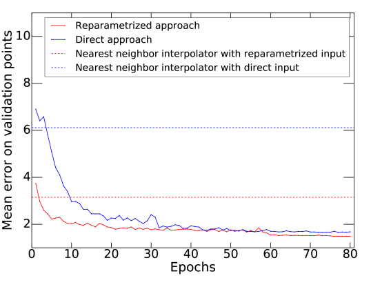
(a)

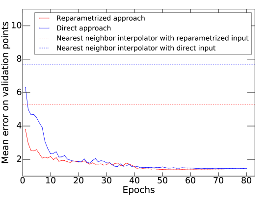
(b)

Figure 12: Progression of the mean absolute error the direct and reparametrized neural networks achieve on the validation set after each training iteration for 8 TeV (a) and 13 TeV (b).

In the center of mass frame, this maximum was calculated with the term,

$$E^{\text{max}}_{i}=\sqrt{\frac{(m_{k}^{2}-(\sum_{j}m_{j}+m_{i})^{2})(m_{k}^{2}-(\sum_{j}m_{j}-m_{i})^{2})}{(2m_{k})^{2}}+m_{i}^{2}}\,.$$ (3)

$E^{\text{max}}_{i}$ gives the maximum energy of daughter particle $i$ with mass $m_{i}$ in the decay $k\rightarrow i+\{j\}$ in the center-of-mass of the mother $k$. $m_{k}$ is the mass of the mother particle while $m_{j}$ represents the mass of the other daughter particle(s) $j$. This term is fast to calculate and the same for any number of daughter particles.

In the next step, the energy of $i$ must be boosted from the center of mass frame of the mother $k$ into the lab frame:

$$E^{\text{max, Lab}}_{i}=\gamma_{k}\;E^{\text{max}}_{i}\,.$$ (4)

Here, the boost $\gamma_{k}$ depends on the energy of the mother $k$ as measured in the lab-frame which we have estimated at an earlier stage in the decay chain, $\gamma_{k}=E^{\text{Lab}}_{k}/m_{k}\approx E^{\text{max, Lab}}_{k}/m_{k}$. For the initial mother (heaviest) particle in the decay chain, we assumed that this was produced at rest and consequently, $E^{\text{max, Lab}}_{\text{initial}}$ was fixed to $m_{\text{initial}}$.

During averaging across all decay trees, not only the mean of the parameters but also the standard deviation was calculated and used as an input. The motivation for such a parameter can easily be understood if for example we consider two new physics scenarios, one which always produces a single lepton in the final state, while the other produces four leptons but only in 25% of decay chains. Both of these scenarios have a mean number of leptons equal to one but if we have a signal region that requires 4-leptons, clearly only the second scenario will satisfy such an analysis.

The set of inputs in the reparametrized approach added 56 parameters but it cannot be trivially assumed that the function mapping the presented parameters to $\chi^{2}_{\rm SN}$ is injective, nor that they are uncorrelated. In a way, the parameters can be seen as a replacement for a first layer of the neural net preparing the inputs to facilitate the modelling process. Their viability should be evaluated based on the results they produce. In theory the reparametrization could be performed for any model, but in practice the cross sections and branching ratios must be obtainable in a timely manner which is why we have restricted ourselves to supersymmetric models where such tools were already available.

4.3 Architecture and training of the reparametrized neural network

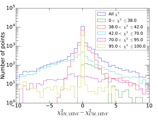
(a)

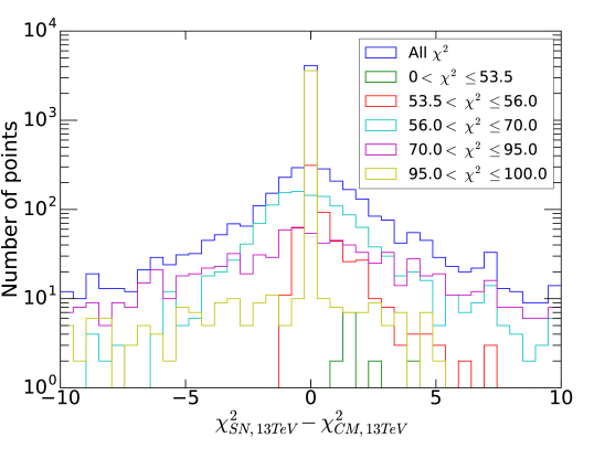
(b)

Figure 13: Performance of the neural network trained on the reparametrized pMSSM-11 points at 8 TeV (a) and 13 TeV (b).

Energy in TeV	Direct approach	Reparameterized approach
8	1.7  (3.1 %)	1.5  (2.7 %)
13	1.5  (2.0 %)	1.3  (1.8 %)

Table 5: Mean errors on the LHC $\chi^{2}$ prediction for both approaches in SCYNet.

For the reparametrized approach, we found that a deeper architecture was preferred with a first layer built from 500 hidden nodes followed by 8 layers of 200 hidden nodes. The added depth, creates additional challenges and required us to alter the hyperparameter setup that we used in the direct approach. Here, rectified linear units (relu) relu were used as activation functions due to them being less prone to the vanishing gradient problem. Due to the larger architecture, overfitting was expected to play a larger role and to counteract this, the regularization term was increased by a factor of 100 to be $\lambda=0.001$, see Eq. (1). In addition the batch size was reduced to 120 (32 for 13TeV) to improve convergence. As in the direct approach, before starting the training, the inputs were again forced to undergo a Z-score normalization. Since the relu activation function is not restricted, the modification described in B was not necessary.

In contrast to the model parameters, the reparametrized inputs were heavily correlated and consequently the inputs were decorrelated by projecting the data into the eigenvectors of the covariance matrix. These mappings were calculated based on the training dataset and then stored to be able to apply the same mappings when evaluating the network. For the training itself, the nAdam adam ; nadam1 ; nadam2 optimizer was used. Compared to the Adam optimizer used in the previous sections, the nAdam optimizer adds Nesterov momentum. The learning rate was initialized a higher value of 0.01 for 8 TeV and 0.002 for 13 TeV. Similar to the batch size, the larger learning rate improved the convergence behaviour in the early stages of the training and was later removed since, as in the direct approach, the learning rate was reduced if the mean error has stopped improving.

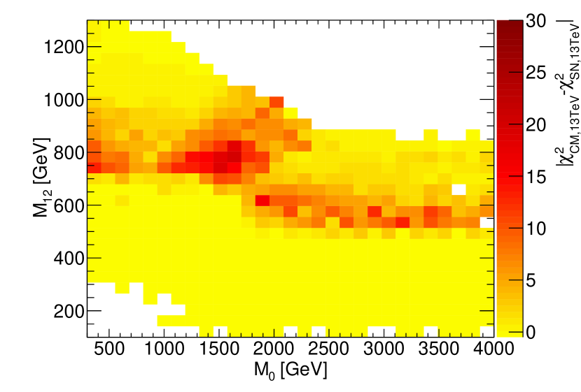
(a)

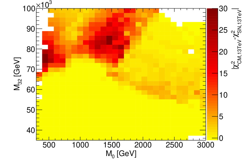
(b)

Figure 14: Performance of the neural network trained on the reparametrized pMSSM-11 points on the cMSSM (a) and AMSB (b). In each bin the mean difference was calculated for all validation points.

4.4 Results of the reparametrized approach to LHC neural nets

During the calculation of the phenomenological parameters, cross sections and branching ratios were calculated. These quantities are related to the expected signal events in each signal region in a much more direct way than the model parameters. Consequently the target quantity of the parametrization, the $\chi^{2}$ derived from the signal counts in each non-overlapping signal region, should be more directly dependent on the input parameters of the reparametrized network. This hypothesis was supported by Figure 12 which showed that a nearest neighbor interpolator improves (in both the 8 TeV and 13 TeV case) when moving from the direct to the reparametrized approach. We interpreted this result as showing that the function mapping the reparameterized inputs to the outputs was flatter.

This improvement directly relates to the performance of neural nets which is given in Table 5 as the total mean error of all networks while the distribution of the mean error has been given in Figure 13. In total, the reparameterized approach on average displayed a lower error. Consequently, as we have shown in Table 4, the reparametrized approach outperformed the direct approach in several $\chi^{2}$ ranges. This is offset by the significantly longer computation time required for each call of the reparametrized net in SCYNet. The dominant component of this computation is the time required by Prospino to calculate the electroweak cross sections. Additional research is now being performed to see if this calculation can be done by a separate neural network. That may allow to bring down the computation time as to be competitive with the direct approach.

The most useful upside of the reparametrized approach was that the used input parameters were chosen in a way which should make them (in principle) model independent. This could allow a network which was trained with one model to be used as prediction tool for a wide variety of models. In Figure 14 we have displayed the performance of the 13 TeV reparametrized network trained with the pMSSM-11 samples when fed with points from the cMSSM and the AMSB. We emphasize here that due to Renormalization Group Equation (RGE) running, both the cMSSM and AMSB models are not subsets of the pMSSM-11 since in general all scalar masses become non-degenerate. In large regions of the parameter space, the network has predicted the model $\chi^{2}$ directly calculated from CheckMATE correctly. However, along the transition region from clearly excluded (in the bottom of the frame) to clearly not excluded (in the top of the frame) a few regions of parameter space display discrepancies.

Model	Only pMSSM-11 samples	Additional pMSSM-19 samples
pMSSM-11	1.32	1.50
CMSSM	2.43	1.92
AMSB	2.44	1.63

Table 6: Performance of the 13 TeV neural network in the reparametrized approach applied to models different from the pMSSM-11 used for training.

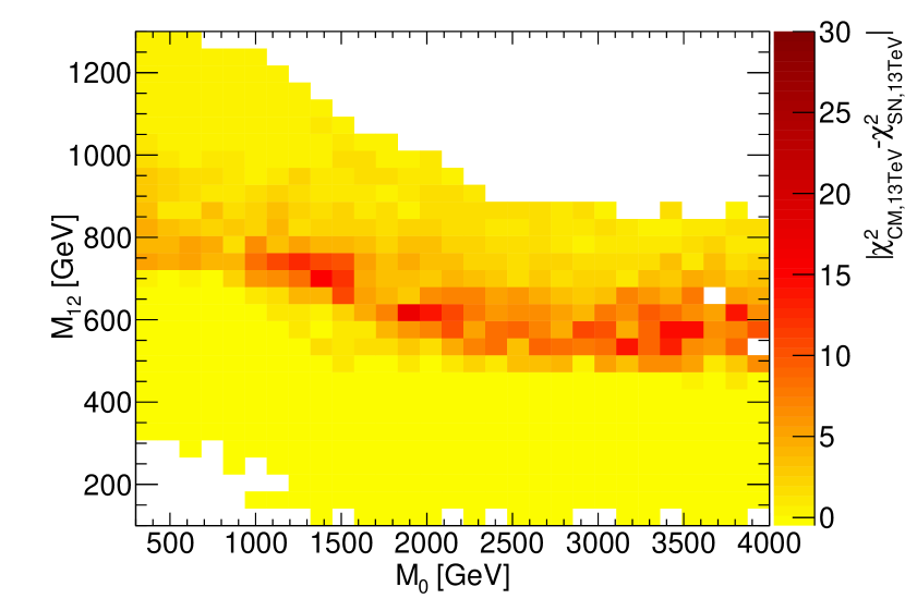
(a)

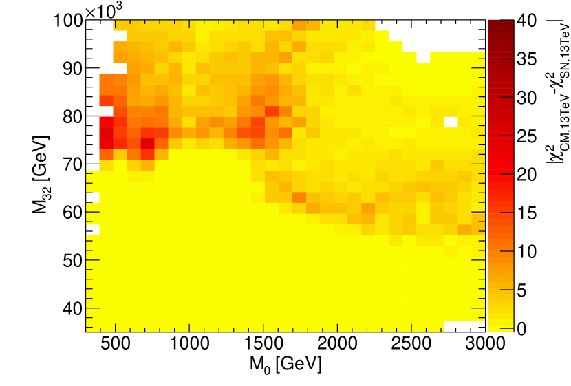
(b)

Figure 15: Performance of the neural network trained on the reparametrized pMSSM-11 points with added samples containing non-degenerate stop sbottom pairs on the cMSSM (a) and AMSB (b). In each bin the mean difference was calculated for all validation points.

In particular a visible anomaly can be seen in the top left of Figure 14 for the AMSB and to a lesser degree the cMSSM. These wrongly predicted points arise because in the pMSSM-11 model, all the stop and the sbottom states (both left- and right-handed) were assumed to be mass degenerate. However, as already alluded to, RGE effects mean that in general this was not the case in the AMSB and cMSSM. In fact, the model points in the anomaly region exhibited a light gluino decaying exclusively into a stop-top pair,

$$\tilde{g}\to\tilde{t}\,t\,,$$ (5)

since the sbottoms are heavier than the gluino here. The stops then further decay, producing either another top quark and a neutralino or a b-quark and a chargino depending on the exact details of the mass spectra via,

$$\tilde{t}\to t\,\tilde{\chi}^{0}\quad\quad\text{or}\quad\quad\tilde{t}\to b\,\tilde{\chi}^{\pm}\,.$$ (6)

Further decays of the top/chargino always produce a $W$-boson, leading to two $W$-bosons per decay chain and four in the complete event. In the considered pMSSM-11 model however, one always additionally observes the gluino decay via an on-shell sbottom and these often do not decay via $W$-Bosons. The average number (and standard deviation) of resonant $W$-Bosons is part of the neural network inputs in the reparametrized approach. Since all decays were averaged during the reparametrization procedure, the pMSSM-11 samples will never contain such a large number of intermediate $W$ bosons. Thus, when we apply the neural network to the AMSB or cMSSM, we no longer interpolate between known parameter points but instead extrapolate to regions of parameter space that the network has never sampled as they were not represented in the training data.

A simple solution to counteract the lack of training data that represents parameter points that only contain light gluinos and stops was to generate additional points in the pMSSM-19 Djouadi:1998di . For these points, the particles charged under SU(3) were forced to obey the following mass relation,

$$m_{\tilde{t}}<m_{\tilde{g}}<m_{\tilde{u},\tilde{d},\tilde{s},\tilde{c},\tilde{b}}$$ (7)

in order to generate training data in the region the reparameterized network fails.

The results of a network trained with the additional pMSSM-19 samples have been displayed in Table 6. The network performs slightly worse on the pMSSM-11 set which was to be expected because the net had to focus on regions of the parameter space which were not present in the pMSSM-11. On the other hand, the mean error of the network applied to the AMSB and cMSSM was significantly reduced. The effects of this can be observed in Figure 15 which has significantly reduced errors compared to Figure 14.

One may notice that anomalous areas still exist with larger errors. This was due to the fact that we did not sample the additional pMSSM-19 points with a high enough density for the neural network to learn the parameter space properly. The points with the worst reconstruction again contain a spectrum with a lighter stop and can be expected to be improved if the pMSSM-19 points were sampled correctly from the beginning.

5 Conclusions

We have developed a neural network regression approach, called SCYNet, for calculating the $\chi^{2}$ of a given SUSY model from a large set of 8 TeV and 13 TeV LHC searches. Previously, such a $\chi^{2}$ calculation would require computational intensive and time consuming Monte Carlo simulations. The SCYNet neural network regression, on the other hand, allows for a fast $\chi^{2}$ evaluation and is thus well suited for global fits of SUSY models.

We have explored two different approaches: in the first, so-called direct, method we simply used the pMSSM-11 parameters as input to the neural network. Within this method the $\chi^{2}$-evaluation for an individual pMSSM-11 parameter point only takes few milliseconds and can thus be used for global pMSSM-11 fits without time penalty. However, the neural network based on the pMSSM-11 parameters cannot be used for any other model. In the second approach, we reparametrized the input to the neural network. Specifically, we used the SUSY masses, cross sections and branching ratios of the pMSSM-11 to estimate signature-based objects, such as particle energies and multiplicities, which provide a more model-independent input for the neural network regression. Although calculating the particle energies and multiplicities for any given parameter point requires ${\cal O}({\rm seconds})$ of computational time, the reparametrized network trained on a particular model can in principle be applied to BSM scenarios the network has not encountered before.

The mean error of both neural network approaches lies in the range of $\Delta\chi^{2}=1.3-1.7$, corresponding to a relative precision between 2% and 3%. This is already very close to the accuracy required for a global fit, where the profile likelihood equivalence between 1 sigma and $\Delta\chi^{2}=1$ implies $\Delta\chi^{2}<1$ as an appropriate goal in precision. For such a complex application with ${\cal O}(50)$ non-overlapping signal regions, the SCYNet implementation represents the most advanced neural network regression for the pMSSM-11 to date.

Applying the reparametrized pMSSM-11 neural network to the cMSSM and AMSB models, we found a few regions of parameter space where the network would fail to predict the correct $\chi^{2}$. As the cMSSM and AMSB models are not subsets of the pMSSM-11, there are cMSSM and AMSB parameter configurations where the network has to extrapolate to regions that were not represented in the training data. We have, however, demonstrated that such problems can be addressed systematically by additional specific training of the network.

Our results motivate the continuation and further improvement of the neural network regression approach to calculating the LHC $\chi^{2}$ for BSM theories. A more accurate approximation to the true LHC likelihood can, for example, be obtained by modeling the probability density functions used for the event generation of the training sample to increase the sampling density in specific regions of parameter space. Furthermore, the treatment of systematic correlations between signal regions should be studied in more detail. The direct approach should be extended to other models, such as the pMSSM-19, so that the neural networks can be used in the corresponding global fits, and the reparameterized neural network regression should be studied further in the context of additional models.

With these improvements in mind, it is possible to decrease the mean error of the SCYNet neural network approach significantly below $\Delta\chi^{2}\approx-2\ln{\cal L}<1$, thus making it a powerful tool for a large variety of global BSM fits.

Appendix A $\chi^{2}$ calculation for one single SR

In this section we explain how to calculate the profile likelihood ratio ($PLR$) for one SR which can be interpreted as the ’$\chi^{2}$’ value used in text.

For a given signal region, the following results are available

• Number of predicted signal events $N_{S}$,

• statistical and total systematic error on signal events $\sigma_{N_{S}}^{\mathrm{stat}}$, $\sigma_{N_{S}}^{\mathrm{sys}}$,

• number of predicted SM events $N_{\mathrm{SM}}$, summed over all background sources,

• statistical and total systematic error on SM events $\sigma_{N_{\mathrm{SM}}}^{\mathrm{stat}}$, $\sigma_{N_{\mathrm{SM}}}^{\mathrm{sys}}$ and

• number of experimentally observed events $N_{E}$.

At first one constructs the likelihood as follows

$$\mathcal{L}(N_{E}|\mu,\nu_{S},\nu_{\mathrm{SM}}):=\frac{e^{-\lambda}}{N_{E}!}\lambda^{N_{E}}\cdot\frac{1}{\sqrt{2\pi}}e^{-\frac{\nu_{S}^{2}}{2}}\cdot\frac{1}{\sqrt{2\pi}}e^{-\frac{\nu_{\mathrm{SM}}^{2}}{2}}.$$ (8)

The first term originates from the Poisson distribution which describes the compatibility of observing $N_{E}$ events if $\lambda$ are expected. Here, $\lambda$ — which itself is a function of the parameters $\mu,\nu_{S},\nu_{\mathrm{SM}}$ explained below — is given as follows:

$$\lambda(\nu_{S},\nu_{SM},\mu):=\mu N_{S}\ e^{\frac{\sigma_{N_{S}}}{N_{S}}\nu_{S}}+N_{\mathrm{SM}}\ e^{\frac{\sigma_{N_{\mathrm{SM}}}}{N_{\mathrm{SM}}}\nu_{\mathrm{SM}}}.$$ (9)

The total uncertainties on signal and background

$$\sigma_{N_{S}} :=\sqrt{\left(\sigma_{N_{S}}^{\mathrm{stat}}\right)^{2}+\left(\sigma_{N_{S}}^{\mathrm{sys}}\right)^{2}},$$ (10)

$$\sigma_{N_{\mathrm{SM}}} :=\sqrt{\left(\sigma_{N_{\mathrm{SM}}}^{\mathrm{stat}}\right)^{2}+\left(\sigma_{N_{\mathrm{SM}}}^{\mathrm{sys}}\right)^{2}}$$ (11)

are reparameterized in terms of dimensionless, Gaussianly distributed nuisance parameters $\nu_{S},\nu_{\mathrm{SM}}$ in Eq. (8). Eq. (9) then describes lognormal distributions of $N_{S},N_{\mathrm{SM}}$ with respective widths $\sigma_{N_{S}},\sigma_{N_{\mathrm{SM}}}$.

In a stochastic picture, we now wish to compare the null hypothesis $H_{0}$ and the alternative hypothesis $H_{1}$:

$$H_{0}:\ \ \parbox{180.00027pt}{The predicted number of signal events, i.e.\ $\mu=1$, coincides well with the experimental observation},$$ (12)

$$H_{1}:\ \ \parbox{180.00027pt}{Any number of signal events, i.e.\ any $\mu$, coincides well with the experimental observation}.$$ (13)

To decide optimally between these two hypotheses, the Neyman-Pearson lemma 10.2307/91247 proposes the profile likelihood ratio

$$PLR:=\frac{\mathcal{L}_{C}}{\mathcal{L}_{G}},$$ (14)

with the respective profile likelihoods defined as

$$\mathcal{L}_{C} := \max_{\nu_{S},\nu_{SM}\in\mathbb{R}}\ \mathcal{L}(\mu=1,\nu_{SM},\nu_{S}),$$ (15)

$$\mathcal{L}_{G} := \max_{\mu,\nu_{S},\nu_{SM}\in\mathbb{R}}\ \mathcal{L}(\mu,\nu_{SM},\nu_{S}).$$ (16)

Here, the constrained likelihood $\mathcal{L}_{C}$ maximizes $\mathcal{L}$ with respect to the nuisance parameters for the null hypothesis with fixed $\mu=1$. In contrast, the global likelihood $\mathcal{L}_{G}$ also varies $\mu$ to find the global maximum of $\mathcal{L}$. Note that the range of allowed $\mu$ is not restricted here and both negative as well as values beyond unity are allowed.

According to Wilk’s theorem wilks1938 , the variable

$$q_{\mu}:=-2\log PLR$$ (17)

is asymptotically $\chi^{2}$ distributed in the limit of large $N_{E}$. We can validate this statement for our setup in the simplified case of negligible uncertainties $\sigma_{N_{S}}$, $\sigma_{N_{\mathrm{SM}}}$. Then, following the prescription above, one finds $q_{\mu}=(N_{S}+N_{\mathrm{SM}}-N_{E})^{2}/(N_{S}+N_{\mathrm{SM}})$ which is indeed the $\chi^{2}$ distribution for one degree of freedom with observation $N_{E}$ and expectation $N_{S}+N_{\mathrm{SM}}$.

We therefore refer the value of $q_{\mu}$ whenever we use the expression ’$\chi^{2}$’ within this work.

Appendix B Modified Z-score normalization

The $\chi^{2}$s which are our targets are called

$$y_{1},\cdots y_{N}\in\mathbb{R}^{+}$$ (18)

in this appendix. We apply the Z-score normalization to them

$$\hat{y}_{i}=\frac{y_{i}-\mu}{\sigma}.$$ (19)

Furthermore we define

$$\hat{y}_{max}:=\max\hat{y}_{i},~{}~{}~{}y_{max}:=\max y_{i}$$ (20)

and finally we normalize again

$$\hat{\hat{y}}_{i}=\frac{\hat{y}_{i}}{\hat{y}_{max}}\in(-1,1).$$ (21)

All targets are therefore in (-1,1).
Usually one chooses $\mu=\frac{1}{N}\sum y_{i}$ and $\sigma=\frac{1}{N-1}\sum(y_{i}-\mu)^{2}$ but this would cause problems with the back transformed outputs of the network. We want the back-transformed outputs of the network to be between the maximum $z_{1}=100$ and the minimum $z_{0}=$ minimum possible LHC $\chi^{2}$.
With the choice

$$\mu=\frac{z_{0}+y_{max}}{2}$$ (22)

$z_{0}$ corresponds to an output value of $\hat{\hat{y}}=-1$.
$z_{1}$ corresponds to an output value of $\hat{\hat{y}}=+1$.
Therefore we choose,

$$\sigma=\frac{1}{N-1}\sum\limits_{i}(y_{i}-(\frac{1}{N}\sum\limits_{j}y_{j}))^{2}$$ (23)

References

- (1) P. Bechtle, et al., Eur. Phys. J. C76(2), 96 (2016). DOI 10.1140/epjc/s10052-015-3864-0
- (2) K.J. de Vries, et al., Eur. Phys. J. C75(9), 422 (2015). DOI 10.1140/epjc/s10052-015-3599-y
- (3) C. Strege, G. Bertone, G.J. Besjes, S. Caron, R. Ruiz de Austri, A. Strubig, R. Trotta, JHEP 09, 081 (2014). DOI 10.1007/JHEP09(2014)081
- (4) A. Djouadi, et al., (1998). URL https://inspirehep.net/record/481987/files/arXiv:hep-ph_9901246.pdf
- (5) M. Drees, H. Dreiner, D. Schmeier, J. Tattersall, J.S. Kim, Comput. Phys. Commun. 187, 227 (2015). DOI 10.1016/j.cpc.2014.10.018
- (6) J.S. Kim, D. Schmeier, J. Tattersall, K. Rolbiecki, Comput. Phys. Commun. 196, 535 (2015). DOI 10.1016/j.cpc.2015.06.002
- (7) D. Dercks, N. Desai, J.S. Kim, K. Rolbiecki, J. Tattersall, T. Weber, (2016)
- (8) M. Abadi, et al. TensorFlow: Large-scale machine learning on heterogeneous systems (2015). URL http://tensorflow.org/. Software available from tensorflow.org
- (9) Theano Development Team, arXiv e-prints abs/1605.02688 (2016). URL http://arxiv.org/abs/1605.02688
- (10) F. Chollet. keras. https://github.com/fchollet/keras (2015)
- (11) A. Buckley, A. Shilton, M.J. White, Comput. Phys. Commun. 183, 960 (2012). DOI 10.1016/j.cpc.2011.12.026
- (12) N. Bornhauser, M. Drees, Phys. Rev. D88, 075016 (2013). DOI 10.1103/PhysRevD.88.075016
- (13) S. Caron, J.S. Kim, K. Rolbiecki, R. Ruiz de Austri, B. Stienen, (2016)
- (14) C.E. Rasmussen, Gaussian Processes in Machine Learning (Springer Berlin Heidelberg, Berlin, Heidelberg, 2004), pp. 63–71. DOI 10.1007/978-3-540-28650-9_4. URL http://dx.doi.org/10.1007/978-3-540-28650-9_4
- (15) G. Bertone, M.P. Deisenroth, J.S. Kim, S. Liem, R. Ruiz de Austri, M. Welling, (2016)
- (16) L. Randall, R. Sundrum, Nucl. Phys. B557, 79 (1999). DOI 10.1016/S0550-3213(99)00359-4
- (17) G.F. Giudice, M.A. Luty, H. Murayama, R. Rattazzi, JHEP 12, 027 (1998). DOI 10.1088/1126-6708/1998/12/027
- (18) J.A. Aguilar-Saavedra, et al., Eur. Phys. J. C46, 43 (2006). DOI 10.1140/epjc/s2005-02460-1
- (19) W. Porod, Comput. Phys. Commun. 153, 275 (2003). DOI 10.1016/S0010-4655(03)00222-4
- (20) K.A. Olive, et al., Chin. Phys. C38, 090001 (2014). DOI 10.1088/1674-1137/38/9/090001
- (21) T.E.W. Group, (2012)
- (22) Y. Amhis, et al., (2012)
- (23) CMS, L. Collaborations, (2013)
- (24) J. Beringer, et al., Phys. Rev. D86, 010001 (2012). DOI 10.1103/PhysRevD.86.010001
- (25) V. Khachatryan, et al., Nature 522, 68 (2015). DOI 10.1038/nature14474
- (26) G. Aad, et al., JHEP 04, 169 (2014). DOI 10.1007/JHEP04(2014)169
- (27) G. Aad, et al., JHEP 05, 071 (2014). DOI 10.1007/JHEP05(2014)071
- (28) Search for supersymmetry in events with four or more leptons in 21 fb-1 of pp collisions at TeV with the ATLAS detector. Tech. Rep. ATLAS-CONF-2013-036, CERN, Geneva (2013). URL https://cds.cern.ch/record/1532429
- (29) G. Aad, et al., JHEP 10, 189 (2013). DOI 10.1007/JHEP10(2013)189
- (30) G. Aad, et al., JHEP 06, 124 (2014). DOI 10.1007/JHEP06(2014)124
- (31) G. Aad, et al., JHEP 06, 035 (2014). DOI 10.1007/JHEP06(2014)035
- (32) G. Aad, et al., JHEP 09, 176 (2014). DOI 10.1007/JHEP09(2014)176
- (33) G. Aad, et al., JHEP 11, 118 (2014). DOI 10.1007/JHEP11(2014)118
- (34) G. Aad, et al., Phys. Rev. D90(5), 052008 (2014). DOI 10.1103/PhysRevD.90.052008
- (35) G. Aad, et al., Eur. Phys. J. C75(7), 299 (2015). DOI 10.1140/epjc/s10052-015-3517-3,10.1140/epjc/s10052-015-3639-7. [Erratum: Eur. Phys. J.C75,no.9,408(2015)]
- (36) G. Aad, et al., Eur. Phys. J. C75(7), 318 (2015). DOI 10.1140/epjc/s10052-015-3661-9,10.1140/epjc/s10052-015-3518-2. [Erratum: Eur. Phys. J.C75,no.10,463(2015)]
- (37) Search for gluinos in events with an isolated lepton, jets and missing transverse momentum at with the ATLAS detector. Tech. Rep. ATLAS-CONF-2015-076, CERN, Geneva (2015). URL https://cds.cern.ch/record/2114848
- (38) G. Aad, et al., Eur. Phys. J. C76(5), 259 (2016). DOI 10.1140/epjc/s10052-016-4095-8
- (39) M. Aaboud, et al., Eur. Phys. J. C76(7), 392 (2016). DOI 10.1140/epjc/s10052-016-4184-8
- (40) A search for Supersymmetry in events containing a leptonically decaying boson, jets and missing transverse momentum in TeV collisions with the ATLAS detector. Tech. Rep. ATLAS-CONF-2015-082, CERN, Geneva (2015). URL http://cds.cern.ch/record/2114854
- (41) M. Aaboud, et al., Phys. Rev. D94(3), 032005 (2016). DOI 10.1103/PhysRevD.94.032005
- (42) Search for production of vector-like top quark pairs and of four top quarks in the lepton-plus-jets final state in collisions at TeV with the ATLAS detector. Tech. Rep. ATLAS-CONF-2016-013, CERN, Geneva (2016). URL http://cds.cern.ch/record/2140998
- (43) Search for pair-production of gluinos decaying via stop and sbottom in events with -jets and large missing transverse momentum in TeV collisions with the ATLAS detector. Tech. Rep. ATLAS-CONF-2015-067, CERN, Geneva (2015). URL http://cds.cern.ch/record/2114839
- (44) V. Khachatryan, et al., Submitted to: JHEP (2016)
- (45) J. Alwall, R. Frederix, S. Frixione, V. Hirschi, F. Maltoni, O. Mattelaer, H.S. Shao, T. Stelzer, P. Torrielli, M. Zaro, (2014). DOI 10.1007/JHEP07(2014)079
- (46) P.M. Nadolsky, H.L. Lai, Q.H. Cao, J. Huston, J. Pumplin, D. Stump, W.K. Tung, C.P. Yuan, Phys. Rev. D78, 013004 (2008). DOI 10.1103/PhysRevD.78.013004
- (47) T. Sjostrand, S. Mrenna, P.Z. Skands, JHEP 05, 026 (2006). DOI 10.1088/1126-6708/2006/05/026
- (48) G. Aad, et al., Phys. Rev. D93(5), 052002 (2016). DOI 10.1103/PhysRevD.93.052002
- (49) T. Sjöstrand, S. Ask, J.R. Christiansen, R. Corke, N. Desai, P. Ilten, S. Mrenna, S. Prestel, C.O. Rasmussen, P.Z. Skands, Comput. Phys. Commun. 191, 159 (2015). DOI 10.1016/j.cpc.2015.01.024
- (50) N. Desai, P.Z. Skands, Eur. Phys. J. C72, 2238 (2012). DOI 10.1140/epjc/s10052-012-2238-0
- (51) W. Beenakker, R. Hopker, M. Spira, P.M. Zerwas, Nucl. Phys. B492, 51 (1997). DOI 10.1016/S0550-3213(97)80027-2
- (52) A. Kulesza, L. Motyka, Phys. Rev. Lett. 102, 111802 (2009). DOI 10.1103/PhysRevLett.102.111802
- (53) A. Kulesza, L. Motyka, Phys. Rev. D80, 095004 (2009). DOI 10.1103/PhysRevD.80.095004
- (54) W. Beenakker, S. Brensing, M. Krämer, A. Kulesza, E. Laenen, I. Niessen, JHEP 12, 041 (2009). DOI 10.1088/1126-6708/2009/12/041
- (55) W. Beenakker, S. Brensing, M.n. Krämer, A. Kulesza, E. Laenen, L. Motyka, I. Niessen, Int. J. Mod. Phys. A26, 2637 (2011). DOI 10.1142/S0217751X11053560
- (56) W. Beenakker, M. Krämer, T. Plehn, M. Spira, P.M. Zerwas, Nucl. Phys. B515, 3 (1998). DOI 10.1016/S0550-3213(98)00014-5
- (57) W. Beenakker, S. Brensing, M. Krämer, A. Kulesza, E. Laenen, I. Niessen, JHEP 08, 098 (2010). DOI 10.1007/JHEP08(2010)098
- (58) W. Beenakker, S. Brensing, M. Krämer, A. Kulesza, E. Laenen, L. Motyka, I. Niessen, Int. J. Mod. Phys. A26, 2637 (2011). DOI 10.1142/S0217751X11053560
- (59) H.K. Dreiner, M. Krämer, J. Tattersall, Europhys. Lett. 99, 61001 (2012). DOI 10.1209/0295-5075/99/61001
- (60) H. Dreiner, M. Krämer, J. Tattersall, Phys. Rev. D87(3), 035006 (2013). DOI 10.1103/PhysRevD.87.035006
- (61) M. Cacciari, G.P. Salam, Phys. Lett. B641, 57 (2006). DOI 10.1016/j.physletb.2006.08.037
- (62) M. Cacciari, G.P. Salam, G. Soyez, Eur. Phys. J. C72, 1896 (2012). DOI 10.1140/epjc/s10052-012-1896-2
- (63) M. Cacciari, G.P. Salam, G. Soyez, JHEP 04, 063 (2008). DOI 10.1088/1126-6708/2008/04/063
- (64) J. Cao, L. Shang, J.M. Yang, Y. Zhang, JHEP 06, 152 (2015). DOI 10.1007/JHEP06(2015)152
- (65) M.R. Buckley, J.D. Lykken, C. Rogan, M. Spiropulu, Phys. Rev. D89(5), 055020 (2014). DOI 10.1103/PhysRevD.89.055020
- (66) J. de Favereau, C. Delaere, P. Demin, A. Giammanco, V. Lemaitre, A. Mertens, M. Selvaggi, JHEP 02, 057 (2014). DOI 10.1007/JHEP02(2014)057
- (67) D.P. Kingma, J. Ba, CoRR abs/1412.6980 (2014). URL http://arxiv.org/abs/1412.6980
- (68) E. Jones, T. Oliphant, P. Peterson, et al. SciPy: Open source scientific tools for Python (2001–). URL http://www.scipy.org/. [Online; accessed <today>]
- (69) A. Buckley, Eur. Phys. J. C75(10), 467 (2015). DOI 10.1140/epjc/s10052-015-3638-8
- (70) W. Beenakker, C. Borschensky, M. Krämer, A. Kulesza, E. Laenen, S. Marzani, J. Rojo, Eur. Phys. J. C76(2), 53 (2016). DOI 10.1140/epjc/s10052-016-3892-4
- (71) W. Beenakker, R. Hopker, M. Spira, P.M. Zerwas, Nucl. Phys. B492, 51 (1997). DOI 10.1016/S0550-3213(97)80027-2
- (72) A. Kulesza, L. Motyka, Phys. Rev. Lett. 102, 111802 (2009). DOI 10.1103/PhysRevLett.102.111802
- (73) A. Kulesza, L. Motyka, Phys. Rev. D80, 095004 (2009). DOI 10.1103/PhysRevD.80.095004
- (74) W. Beenakker, S. Brensing, M. Krämer, A. Kulesza, E. Laenen, I. Niessen, JHEP 12, 041 (2009). DOI 10.1088/1126-6708/2009/12/041
- (75) W. Beenakker, S. Brensing, M. Krämer, A. Kulesza, E. Laenen, L. Motyka, I. Niessen, Int. J. Mod. Phys. A26, 2637 (2011). DOI 10.1142/S0217751X11053560
- (76) W. Beenakker, M. Krämer, T. Plehn, M. Spira, P.M. Zerwas, Nucl. Phys. B515, 3 (1998). DOI 10.1016/S0550-3213(98)00014-5
- (77) W. Beenakker, S. Brensing, M. Krämer, A. Kulesza, E. Laenen, I. Niessen, JHEP 08, 098 (2010). DOI 10.1007/JHEP08(2010)098
- (78) M. Krämer, T. Plehn, M. Spira, P.M. Zerwas, Phys. Rev. Lett. 79, 341 (1997). DOI 10.1103/PhysRevLett.79.341
- (79) M. Krämer, T. Plehn, M. Spira, P.M. Zerwas, Phys. Rev. D71, 057503 (2005). DOI 10.1103/PhysRevD.71.057503
- (80) A. Alves, O. Eboli, T. Plehn, Phys. Lett. B558, 165 (2003). DOI 10.1016/S0370-2693(03)00266-1
- (81) T. Plehn, Phys. Rev. D67, 014018 (2003). DOI 10.1103/PhysRevD.67.014018
- (82) A. Alves, T. Plehn, Phys. Rev. D71, 115014 (2005). DOI 10.1103/PhysRevD.71.115014
- (83) G.P. Lepage, Journal of Computational Physics 27, 192 (1978). DOI 10.1016/0021-9991(78)90004-9
- (84) V. Nair, G.E. Hinton, in Proceedings of the 27th International Conference on Machine Learning (2010), pp. 807–814
- (85) D.P. Kingma, J. Ba, CoRR abs/1412.6980 (2014). URL http://arxiv.org/abs/1412.6980
- (86) I. Sutskever, J. Martens, G.E. Dahl, G.E. Hinton, in Proceedings of the 30th International Conference on Machine Learning, vol. 28 (2013), vol. 28, pp. 1139–1147
- (87) T. Dozat, (2015). URL http://cs229.stanford.edu/proj2015/054_report.pdf
- (88) J. Neyman, E.S. Pearson, Philosophical Transactions of the Royal Society of London. Series A, Containing Papers of a Mathematical or Physical Character 231, 289 (1933). URL http://www.jstor.org/stable/91247
- (89) S.S. Wilks, Ann. Math. Statist. 9(1), 60 (1938). DOI 10.1214/aoms/1177732360. URL http://dx.doi.org/10.1214/aoms/1177732360