Dual Maxwellian-Kappa modelling of the solar wind electrons:
new clues on the temperature of Kappa populations

Abstract

Context. Recent studies on Kappa distribution functions invoked in space plasma applications have emphasized two alternative approaches which may assume the temperature parameter either dependent or independent of the power-index $\kappa$. Each of them can obtain justification in different scenarios involving Kappa-distributed plasmas, but direct evidences supporting any of these two alternatives with measurements from laboratory or natural plasmas are not available yet.

Aims. This paper aims to provide more facts on this intriguing issue from direct fitting measurements of suprathermal electron populations present in the solar wind, as well as from their destabilizing effects predicted by these two alternating approaches.

Methods. Two fitting models are contrasted, namely, the global Kappa and the dual Maxwellian-Kappa models, which are currently invoked in theory and observations. The destabilizing effects of suprathermal electrons are characterized on the basis of a kinetic approach which accounts for the microscopic details of the velocity distribution.

Results. In order to be relevant, the model is chosen to accurately reproduce the observed distributions and this is achieved by a dual Maxwellian-Kappa distribution function. A statistical survey indicates a $\kappa$-dependent temperature of the suprathermal (halo) electrons for any heliocentric distance. Only for this approach the instabilities driven by the temperature anisotropy are found to be systematically stimulated by the abundance of suprathermal populations, i.e., lowering the values of $\kappa$-index.

1 Introduction

Kappa modelling is a widely exploited technique for space plasma diagnosis and kinetic analysis (Pierrard & Lazar, 2010; Livadiotis & McComas, 2013). The Kappa ($\kappa$-)distribution function is nearly Maxwellian at low energies and decreases as a power-law at higher energies, enabling a satisfactory overall (global) description of the velocity distributions of plasma particles measured in the solar wind (Vasyliunas, 1968; Christon et al., 1989; Collier et al., 1996; Maksimovic et al., 1997). The power-index $\kappa$ quantifies the presence of suprathermal (non-Maxwellian) populations, which enhance the high energy tails of the distributions. Alternatively, the same Kappa power-laws have also been used to reproduce only the high-energy tails (also known as the halo component), while the core of the distribution is well fitted by a standard Maxwellian (Maksimovic et al., 2005; Štverák et al., 2008; Pierrard et al., 2016).

Recent studies on global Kappa models have emphasized two distinct alternatives, namely, assuming the temperature (fitting) parameter either dependent or independent of the $\kappa$-index (Lazar et al., 2015a, 2016a). Modelling with a $\kappa$-independent temperature is convenient in computations, and it is therefore very much invoked in theoretical predictions on dispersion and stability properties of Kappa distributed plasmas, see the reviews by Hellberg et al. (2005) and Pierrard & Lazar (2010). The effects of a varying $\kappa$ (including the Maxwellian limit $\kappa\to\infty$) are also easier to parametrize if temperature is taken constant. However, for studies intended to outline the effects of suprathermal populations, Lazar et al. (2015a, 2016a) have shown that only the approach assuming a $\kappa$-dependent temperature may provide a fairly rigorous comparison of the global Kappa describing the observed distribution, with the cooler Maxwellian $\kappa\to\infty$ limit reproducing the core of the distribution. Moreover, only in this case the instabilities driven by the kinetic anisotropies of plasma particles are systematically stimulated by the suprathermals (i.e., lowering the values of $\kappa$), confirming the expectation that these populations should contribute with an additional free energy (Lazar et al., 2015a, 2016b). From a different perspective including, for instance, the origin of Kappa distributions, there are processes responsible for the formation of suprathermal tails, e.g., particle energization by the wave turbulence, which may imply a $\kappa$-independent evolution of the velocity distributions (Yoon, 2014; Lazar et al., 2016a). In this case, the high-energy tails are counter-balanced by a low-velocity enhancement, so that the temperature remains indeed independent of parameter $\kappa$.

A global Kappa distribution implies a reduced number of parameters and is, therefore, easy to manipulate in observational and theoretical analyses. However, a global Kappa does not always provide a good fit to the observed distributions, as we will see here below, e.g., the analysis in section 2 (also Figs. 1 and 2), which suggests that a global Kappa is just a simplified (or idealized) approach that artificially constrains the core and suprathermal populations to be described by the same parameters, e.g., density, temperature, anisotropy (not fully justified yet, although some studies in this direction have been done by Leubner (2004); Lazar et al. (2015a, 2016a)). It may be, therefore, that fitting measurements of the observed distributions with global Kappa models can not provide relevant evidences to support any of the two alternatives of a temperature either dependent or independent of the power-index $\kappa$.

More complex models that combine distinct components are in general more accurate in reproducing the distributions measured in the solar wind, and may, therefore, unveil details of the observed distributions. For instance, the nonstreaming distributions detected in the slow winds and at sufficiently large distances from the Sun (Maksimovic et al., 2005) are expected to be better described by a dual model comprising a standard Maxwellian distribution function to reproduce the core at low energies, and a Kappa power-law to fit the suprathermal tails (halo component) of the distribution (see Figs. 1 and 2). In the fast winds the observed distributions become asymmetric (see Fig. 3), and to describe them we need an additional component (called strahl) streaming along the magnetic field direction. Such complex models have already been invoked in observational analyses in order to quantify the main physical properties of these components, e.g., densities, relative drifts, temperatures, and even temperature anisotropies (Maksimovic et al., 2005; Nieves-Chinchilla & Viñas, 2008; Štverák et al., 2008; Viñas et al., 2010; Pierrard et al., 2016). The halo component can be called suprathermal as long it is well reproduced by Kappa power-laws with sufficiently low values of $\kappa$, i.e., $\kappa<10$. Otherwise, for higher values, i.e., $\kappa>10$, the halo component appears to be thermalized and well described by a Maxwellian, but it remains a distinct component, being, in general, less dense but hotter than the core. In this case, the overall distribution can be described by a two-Maxwellians model, as a limiting $\kappa\to\infty$ case of a dual Maxwellian-Kappa representation. Although the existence of a halo component with $\kappa>10$ is not so evident from observations, a two-Maxwellians model has already been invoked in theoretical predictions on the dispersion and stability of space plasmas (Gary et al., 1975, 1994) as well as in observational analyses (Feldman et al., 1975; Pilipp et al., 1987) and in comparisons with global Kappa (Maksimovic et al., 1997). Note that this Maxwellian limit ($\kappa\to\infty$) of a Kappa describing only the halo component is completely distinct from the Maxwellian fit to the core, and a correlation between these two is not justified in this case (as for a global Kappa modelling, where the Maxwellian limit may need to reproduce the core of the distribution to compare with the global Kappa and emphasize the effects of the suprathermals).

When the core and suprathermal components are anisotropic, e.g., due to temperature anisotropies or relative drifts, a dual Maxwellian-Kappa modelling becomes complicated to deal with, even in numerical computations. Recently, an important progress has been made for overcoming this challenge in studies of the stability and relaxation of a dual core-halo plasma with intrinsic temperature anisotropies (Lazar et al., 2014, 2015b; Shaaban et al., 2016). Both interpretations were adopted for the anisotropic halo modelled by a bi-Kappa with temperatures being either dependent or independent of the power-index $\kappa$. The results from these studies were again favorable to a Kappa model with a $\kappa$-dependent temperature, since only this approach provided a systematic stimulation of the instabilities in the presence of suprathermals.

The present paper aims to provide additional insight into these properties of Kappa distributed plasmas as they are revealed by observational data. As discussed above, there are two fitting models widely invoked in theory and observations, namely, the global Kappa and the dual Maxwellian-Kappa models. In section 2 we describe them mathematically and analyze qualitatively their accuracy in reproducing the solar wind observational data. Particularly relevant for our analysis is the Kappa model that better reproduces the observed distributions. This model is then considered for fitting to more than 100 000 velocity distributions measured in the ecliptic within an wide interval of heliocentric distance between 0.3 and 4.0 AU. Determined as fitting parameters the temperature and the power-index $\kappa$ are subjected to a statistical analysis that enables us to extract the relationship between them. The $\kappa$-dependency indicated by the observations for the temperature of Kappa populations is used in section 3 for a kinetic analysis of the electromagnetic instabilities driven by the temperature anisotropy. These instabilities can explain the enhanced fluctuations observed in the solar wind, see the review by Zimbardo et al. (2010) and references therein. The results of our study are summarized and discussed in section 4.

2 Refined models from the observations

2.1 Global Kappa vs. dual Maxwellian-Kappa

Fluxes of plasma particles measured in-situ in the solar wind are transformed into the frame of bulk flow, such that, in the absence of any differential streaming, the velocity distributions are almost symmetric in the Sun-ward and anti-Sun-ward directions, without indications of any additional strahl (or streaming) component (see examples in Figs. 1 and 2). One intriguing feature that makes them impossible to describe with standard Maxwellian models are the enhanced high-energy tails, known as suprathermal tails. Instead, the Kappa (Lorentzian) power-laws are used to reproduce the suprathermal tails of the observed distributions, and this can be done in two distinct ways. Thus, a Kappa power-law (subscript $\kappa$) is used either as a global model (subscript $GK$) to fit the entire distribution

$$f_{GK}(v_{\parallel},v_{\perp})=nf_{\kappa}(v_{\parallel},v_{\perp}),$$ (1)

or to describe only the suprathermal halo (subscript $h$) component

$$f_{h}(v_{\parallel},v_{\perp})=f_{\kappa}(v_{\parallel},v_{\perp}).$$ (2)

In the second case the core (subscript $c$) fitting is a Maxwellian (subscript $M$)

$$f_{c}(v_{\parallel},v_{\perp})=f_{M}(v_{\parallel},v_{\perp}),$$ (3)

and the resulting model to describe the entire distribution $f$ is a dual Maxwellian-Kappa (subscript $MK$)

$$f_{MK}(v_{\parallel},v_{\perp})=n_{c}f_{c}(v_{\parallel},v_{\perp})+n_{h}f_{h}(v_{\parallel},v_{\perp}),$$ (4)

Since kinetic modelling deals with homogeneous plasma systems in general, in the above $n$ is the total number density of plasma particles (of given species), and $n_{c}$ and $n_{h}$ are the number densities of the core and halo components, respectively. Moreover, in magnetized plasmas from space the velocity distributions are in general gyrotropic (without a major anisotropy in the plane transverse to the magnetic field) allowing us to describe them in polar coordinates $(v_{x},v_{y},v_{z})=(v_{\perp}\cos\phi,v_{\perp}\sin\phi,v_{\parallel})$ with $\parallel$ and $\perp$ denoting directions relative to the stationary magnetic field. Gyrotropic distribution functions reduce the analysis to only two variables in velocity space and enable us to quantify the principal anisotropies reported by the observations, e.g., the bi-axis temperature anisotropies $T_{\perp}\neq T_{\parallel}$ combined or not with the field-aligned streams (also known as strahls).

Relevant for the nonstreaming distributions observed in the solar wind is the well-known bi-Kappa distribution function (Summers & Thorne, 1991; Lazar et al., 2015a)

$$f_{\kappa}(v_{\parallel},v_{\perp}) = {1\over\pi^{3/2}\theta_{\perp}^{2}\theta_{\parallel}}\,{\Gamma(\kappa+1)\over\kappa^{3/2}\Gamma(\kappa-1/2)}\left(1+{v_{\parallel}^{2}\over\kappa\theta_{\parallel}^{2}}+{v_{\perp}^{2}\over\kappa\theta_{\perp}^{2}}\right)^{-\kappa-1}$$ (5)

$$= \left[m\over\pi k_{B}(2\kappa-3)\right]^{3/2}{1\over T_{\perp}\sqrt{T_{\parallel}}}{\Gamma(\kappa+1)\over\Gamma(\kappa-1/2)}$$

$$\times \left[1+{m\over k_{B}(2\kappa-3)}\left({v_{\parallel}^{2}\over T_{\parallel}}+{v_{\perp}^{2}\over T_{\perp}}\right)\right]^{-\kappa-1},$$

where $v_{\|}$ and $v_{\perp}$ denote particle velocity parallel and perpendicular w.r.t. a large-scale magnetic field, $m$ is particle mass, $k_{B}$ the Boltzmann constant, $\Gamma$ is the Gamma function, the power-index $\kappa\in(3/2,\infty]$, $T_{\|,\perp}$ and $\theta_{\|,\perp}$ the corresponding temperatures and thermal velocities, which are related by

$$T_{\parallel}\equiv{2m\over 2k_{B}}\int d{\bf v}v_{\parallel}^{2}f_{\kappa}(v_{\parallel},v_{\perp})={\kappa\over\kappa-3/2}{m\theta_{\parallel}^{2}\over 2k_{B}},$$ (6)

$$T_{\perp}\equiv{m\over 2k_{B}}\int d{\bf v}v_{\perp}^{2}f_{\kappa}(v_{\parallel},v_{\perp})={\kappa\over\kappa-3/2}{m\theta_{\perp}^{2}\over 2k_{B}}.$$ (7)

This bi-Kappa model is invoked in both fitting techniques, either as a global model to describe the entire distribution (Vasyliunas, 1968; Christon et al., 1989; Collier et al., 1996; Maksimovic et al., 1997), or to fit partially, only the suprathermal tails of the distribution (Maksimovic et al., 2005; Nieves-Chinchilla & Viñas, 2008; Štverák et al., 2008; Pierrard et al., 2016).

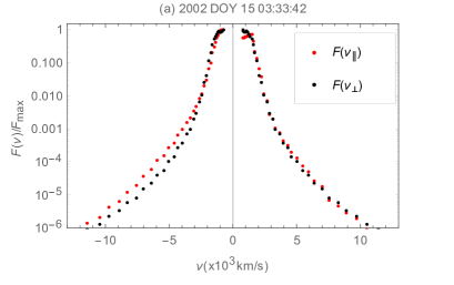
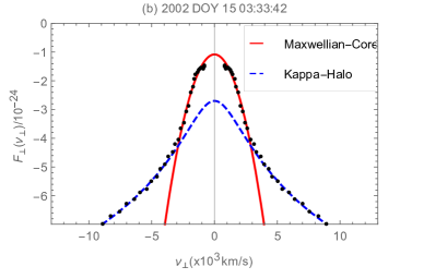
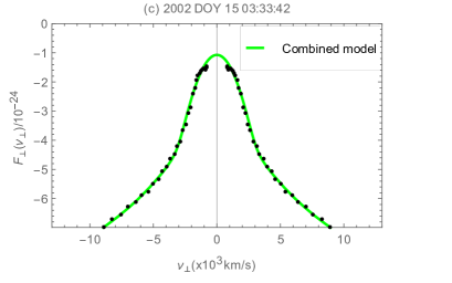
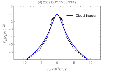
Figure 1: Nonstreaming electron velocity distribution $F$ [cm${}^{-}6$ s$63$] measured by Ulysses in the slow wind in 2002 on DOY 15 03:33:42: (a) parallel and perpendicular cuts; (b) Maxwellian fit to the core and Kappa fit to the halo suprathermal tails; (c) combined (resultant) Maxwellian-Kappa model fitting the entire distribution; (d) global Kappa model fitting the entire distribution.

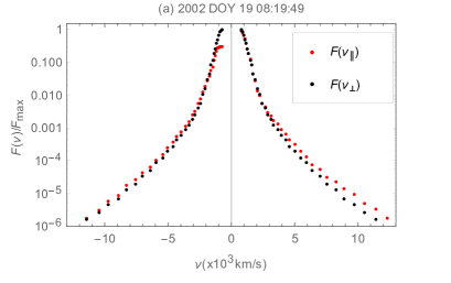
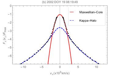
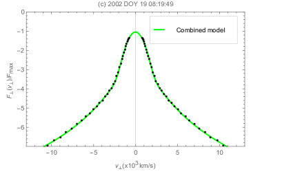
Figure 2: Nonstreaming electron velocity distribution $F$ [cm${}^{-}6$ s$63$] measured by Ulysses in the slow wind in 2002 on DOY 19 08:19:49: (a) parallel and perpendicular cuts; (b) Maxwellian fit to the core and Kappa fit to the halo suprathermal tails; (c) combined (resultant) Maxwellian-Kappa model fitting the entire distribution; (d) global Kappa model fitting the entire distribution.

The low-energy core is well reproduced by a bi-Maxwellian (e.g., in Pilipp et al. (1987))

$$f_{M}(v_{\parallel},v_{\perp})={1\over\pi^{3/2}w_{\parallel}w_{\perp}^{2}}\,\exp\left(-{v_{\parallel}^{2}\over w_{\parallel}^{2}}-{v_{\perp}^{2}\over w_{\perp}^{2}}\right),$$ (8)

where $w_{\parallel,\perp}$ are thermal velocities defined by the temperatures as moments of second order

$$T_{\parallel}\equiv{2m\over 2k_{B}}\int d{\bf v}v_{\parallel}^{2}f_{M}(v_{\parallel},v_{\perp})={mw_{\parallel}^{2}\over 2k_{B}},$$ (9)

$$T_{\perp}\equiv{m\over 2k_{B}}\int d{\bf v}v_{\perp}^{2}f_{M}(v_{\parallel},v_{\perp})={mw_{\perp}^{2}\over 2k_{B}}.$$ (10)

The so-called global Kappa approach from Eq. (1) implies a reduced number of parameters and is, therefore, preferred in computations, while a more complex, dual Maxwellian-Kappa as defined in Eq. (4) is expected to reproduce better the observations, although direct comparisons with global Kappa fittings are not reported yet (at least to our knowledge). In Figs. 1 and 2 we compare these two fitting models as obtained for the electron velocity distributions measured by Ulysses in January 2002 (dotted lines), two events on DOY 15 03:33:42 and DOY 19 08:19:49, respectively. These distributions are chosen to be almost isotropic, i.e., with insignificant differences between parallel (red dots) and perpendicular (black dots) cuts, see top panels a, such that fittings to the perpendicular cut are representative for the entire distribution.

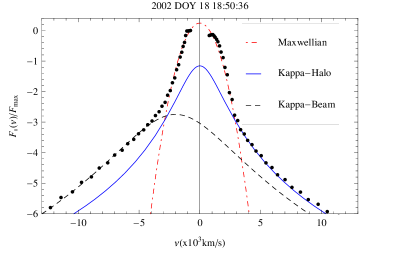
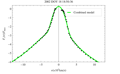
Figure 3: Asymmetric electron distribution $F$ [cm${}^{-}6$ s$63$] measured by Ulysses in 2002 DOY 18 18:50:36: (a) Maxwellian fit to the core, Kappa fit the halo suprathermal tails, and a drifting Kappa fit to the streaming (strahl) component; (b) combined (resultant) model fitting the entire distribution.

The global Kappa fit is displayed in the bottom panels (solid blue lines), and the dual Maxwellian-Kappa fit is explicitly shown in the middle panels: in the second panel from top we have the core (solid red lines) and halo (blue dashed lines) fits and these two are then combined as a dual Maxwellian-Kappa fit in the third panel (solid green lines). Now, a direct comparison of these two fitting models becomes possible just by analyzing the last two bottom panels in Figs. 1 and 2. It is obvious that in both events the observed distribution is better reproduced by a dual Maxwellian-Kappa approach than a global Kappa. Note that in Fig. 2 a global Kappa provides a better fit to the observed distribution than in Fig. 1, but in both these two cases the global Kappa fits are visibly less accurate than those obtained with a dual Maxwellian-Kappa approach. In this case the effects of suprathermals may simply be outlined by a direct comparison between the dual model $f_{MK}$ and the Maxwellian fit $f_{M}$ to the core, and there is no need to consider the Maxwellian limit $\kappa\to\infty$ of the Kappa component.

The fact that a dual model is more accurate may simply suggest the existence of two distinct components, namely, a low-energy core population and a suprathermal Kappa-distributed halo. There is probably no other possibility to make distinction between these components, which may have different origins in the solar corona (Pierrard et al., 1999) or in the solar wind (Maksimovic et al., 2005). On the other hand, these two components are expected to be strongly correlated, especially by the collective effects of plasma particles which should tend to diminish differences between them. However, this is not always confirmed or evident from observations, which show, for instance, an electron halo enhancing with the radial distance from the Sun on the expense of the more anisotropic strahl which is diminished in almost the same measure (Maksimovic et al., 2005). In this case an explanation may be offered by the instabilities and amplified fluctuations selfgenerated by the strahl, which can isotropize the strahl, scattering the particles and thus feeding the more isotropic suprathermal halo. A dual core-halo model is relevant not only in the slow winds when the flowing (bulk) speed is sufficiently low (i.e., $V_{\rm SW}<360$ km s^-1), and the relative density of the strahl is negligibly small $n_{s}<n_{h}<n_{c}$ (Lazar et al., 2015b), but according to Maksimovic et al. (2005) it may also describe any slow or fast wind conditions at sufficiently large heliocentric distances, e.g., beyond 1 AU where the strahl component is markedly reduced. A dual Maxwellian-Kappa remains a major component in the fast winds, when the velocity distribution exhibits an additional streaming component (called strahl). In Fig. 3 we display an example of velocity distribution of electrons measured during a fast solar wind by Ulysses in January 2002. In this case the best fitting model contains three components: a Maxwellian core, a Kappa halo, and a drifting-Kappa strahl (or beam of particles).

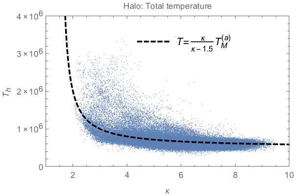
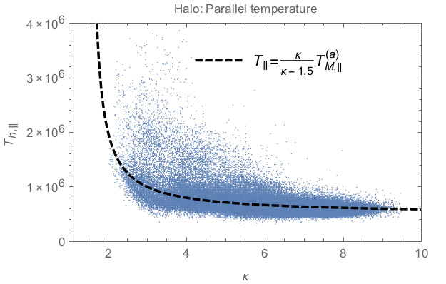
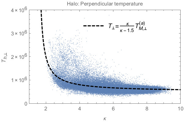
Figure 4: Scatter plots (blue dots) of the halo temperature $T$ [K] vs. $\kappa$-index, measured in the ecliptic (0.3 AU $\leqslant R<$ 4 AU): total temperature (top), and the components, parallel temperature (middle), and perpendicular temperature (bottom). The temperatures predicted by the Eqs. (15)–(17) as functions of $\kappa$ parameter are overplotted with dashed lines.

2.2 The Kappa (halo) temperature from observations

If a $\kappa$-dependency exists for the temperature of Kappa population, then this must be revealed by the observational data. In order to be relevant the Kappa model should accurately reproduce the measured distribution, and here above we have demonstrated that this condition is satisfied by a dual Maxwellian-Kappa model, with Kappa distribution function fitting only the suprathermal (halo) tails.

Štverák et al. (2008) have used the same dual Maxwellian-Kappa model from Eq. (4) to determine the principal moments of the electron distributions measured in the solar wind. The dual model was fitted to more than 100 000 velocity distributions measured by three different spacecraft missions (Helios 1, Cluster II, and Ulysses) in the ecliptic at different heliocentric distances in the interval 0.3–3.95 AUs. Details about the electron analyzers and the methods of correction and reconstruction of the 3D velocity distributions are given in Štverák et al. (2008) and some references therein. Here we make use of the same data set, and investigate the temperature parameters determined for the Kappa (halo) populations. Fig. 4 displays scatter plots (with blue dots) of the temperatures determined for the electron halo (subscript $h$) vs. the corresponding values of the power-index $\kappa$: total temperature ($T_{h}$) in the top panel, parallel ($T_{h,\parallel}$) and perpendicular ($T_{h,\perp}$) temperatures in the middle and bottom panels, respectively. One dimensional fits provide temperature components $T_{h,\parallel}$ and $T_{h,\perp}$, enabling us to calculate $T_{h}=T_{h,\parallel}/3+2T_{h,\perp}/3$.

For each panel in Fig. 4 the spread of data points is very similar and we can analyze them generically. The data points concentrate along a curve which clearly shows that temperature is not constant but varies as a function of $\kappa$. Thus, the temperature of Kappa population decreases with increasing power-index $\kappa$, with the allure of an asymptotic decrease towards the Maxwellian limit $\kappa\to\infty$. In this limit of a very large $\kappa\to\infty$ the bi-Kappa reproducing the halo components reduces to a bi-Maxwellian (similar to that reproducing the core component). However, Lazar et al. (2016a) have shown that any Kappa distribution function admits two distinct Maxwellian limits:

(a)

a cooler Maxwellian limit corresponding to the approach with a $\kappa$-dependent temperature

$$f_{M}^{(a)}=\lim_{\kappa\to\infty}f_{\kappa}(v_{\parallel},v_{\perp})={1\over\pi^{3/2}\theta_{\parallel}\theta_{\perp}^{2}}\exp\left(-{v_{\parallel}^{2}\over\theta_{\parallel}^{2}}-{v_{\perp}^{2}\over\theta_{\perp}^{2}}\right),$$ (11)

with thermal velocities $\theta_{\parallel,\perp}$ determined in this case by lower temperatures

$$T_{M,\parallel}^{(a)}=\lim_{\kappa\to\infty}T_{\parallel}={m\theta_{\parallel}^{2}\over 2k_{B}}\leqslant{\kappa\over\kappa-3/2}{m\theta_{\parallel}^{2}\over 2k_{B}}=T_{\parallel},$$ (12)

$$T_{M,\perp}^{(a)}=\lim_{\kappa\to\infty}T_{\perp}={m\theta_{\perp}^{2}\over 2k_{B}}\leqslant{\kappa\over\kappa-3/2}{m\theta_{\perp}^{2}\over 2k_{B}}=T_{\perp}.$$ (13)

(b)

the second limit corresponds to the approach with a constant temperature, not dependent on $\kappa$:

$$f_{M}^{(b)} = \lim_{\kappa\to\infty}f_{\kappa}(v_{\parallel},v_{\perp})$$ (14)

$$= \left({m\over 2\pi k_{B}}\right)^{3/2}{1\over\sqrt{T_{\parallel}}T_{\perp}}\exp\left[-{m\over 2k_{B}}\left({v_{\parallel}^{2}\over T_{\parallel}}+{v_{\perp}^{2}\over T_{\perp}}\right)\right],$$

where $T_{M,\parallel}^{(b)}=T_{\parallel}$ and $T_{M,\perp}^{(b)}=T_{\perp}$.

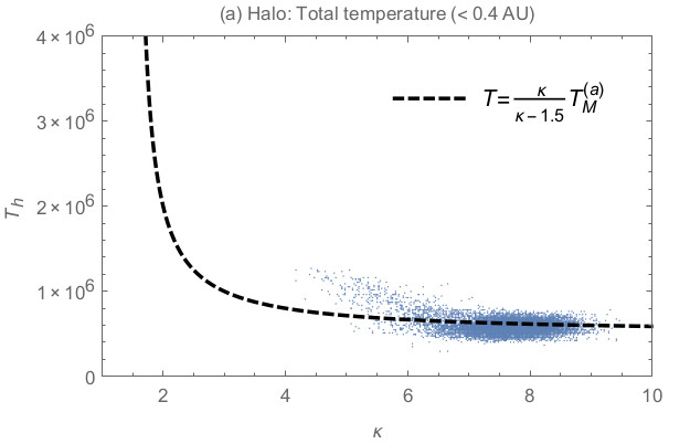
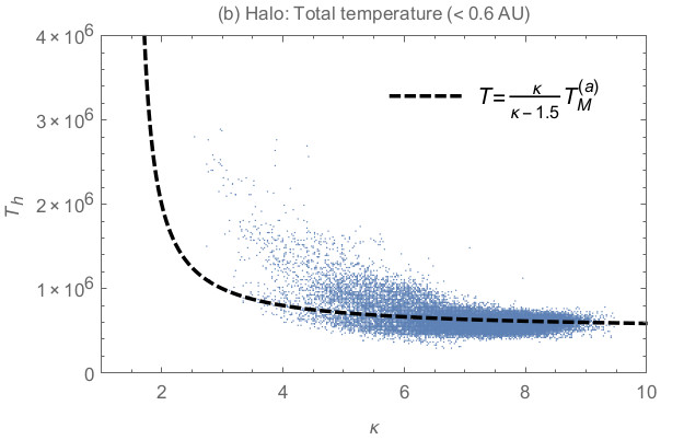
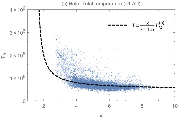
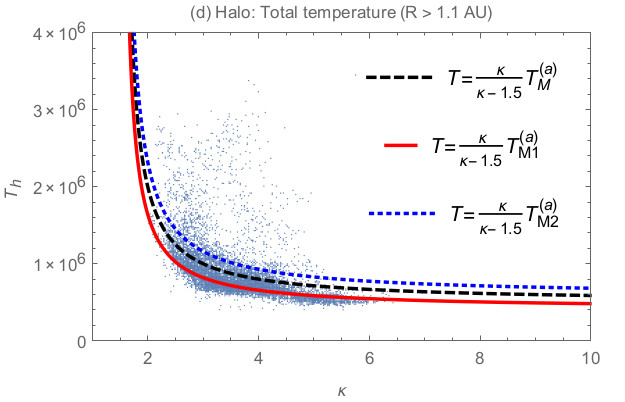
Figure 5: Scatter plots (blue dots) of the halo (total) temperature $T$ [K] vs. $\kappa$-index, measured in different intervals of heliocentric distances $R$ (selected from the data set in Fig. 4): (a) $0.3<R<0.4$ AU, (b) $<0.6$ AU, (c) $\sim 1$ AU (0.9 AU $\leqslant R\leqslant$ 1.1 AU), (d) $R>1.1$ AU. Fitting curves are explained in the text.

The observations indicate a $\kappa$-dependent temperature, when the components $T_{\parallel,\perp}$ can be defined in terms of their Maxwellian limits $T_{M,\parallel,\perp}^{(a)}$ as follows

$$T_{\parallel}={\kappa\over\kappa-3/2}{m\theta_{\parallel}^{2}\over 2k_{B}}={\kappa\over\kappa-1.5}T_{M,\parallel}^{(a)},$$ (15)

$$T_{\perp}={\kappa\over\kappa-3/2}{m\theta_{\perp}^{2}\over 2k_{B}}={\kappa\over\kappa-1.5}T_{M,\perp}^{(a)}.$$ (16)

and a similar relation is obtained for the total temperature

$$T={\kappa\over\kappa-3/2}T_{M}^{(a)}.$$ (17)

Using these relations to fit to the observations, see the dashed curves in Fig. 4, we find for the Maxwellian limits $T_{M}^{(a)}\simeq T_{M,\parallel}^{(a)}\simeq T_{M,\perp}^{(a)}=5\times 10^{5}$ K. We should point out that the accumulation of data aligns with these dashed curves very well, which confirms the validity of $\kappa$-dependency found in Eqs. (15)–(17). However, the power-index $\kappa$ describing the electron halo population in the solar wind does not take very large values, being limited to $\kappa<10$. Therefore, for a rigorous interpretation of the solar wind electrons, a two-Maxwellian model seems to be not justified, but can be invoked as a limiting case of a dual Maxwellian-Kappa in order to depict and investigate the effects of the suprathermal populations.

Both parameters $T$ and $\kappa$ analyzed here characterize the halo (Kappa) electron component of the solar wind plasma, and should therefore undergo a variation with the radial (heliocentric) distance from the Sun, being naturally conditioned by the solar wind evolution during its expansion in space. Thus, recent studies of the same set of data (Pierrard et al., 2016) have shown significant differences between the core and halo temperatures, and implicitly between their evolutions with heliocentric distance: the core temperature decreases (with a tendency of stabilizing after 2 AU) while the halo temperature increases with radial distance from the Sun (with an apparent saturation at about 3 AU). Normally, the temperature should indeed cool down with the distance from the Sun, as the core temperature is confirming. The increase of the halo temperature is somehow unusual, although it is in perfect agreement with the evolution of the other parameters reported by different observations (Maksimovic et al., 2005; Pierrard et al., 2016), namely, the increase of halo population (i.e, the increase of its relative number density $n_{h}/n_{c}$) at the same time with a decrease of $\kappa$ with radial distance. The halo population seems to be enhanced on the expense of the strahl population, which is eventually scattered and isotropized by the selfgenerated instabilities (collisions are inefficient at large distances in the solar wind). At this point it becomes therefore interesting to check whether such kind of processes may have an influence on the $\kappa$-dependency shown by the halo temperature in the observations.

Fig. 5 is intended to unveil the existence of these influences if they exist, by presenting in detail a radial profile of the halo temperature as a function of the power-index $\kappa$. We made a selection of the data from different heliocentric distances, and plot in four panels with the distance increasing from top panel (a) to bottom panel (d) as follows: (a) $0.3<R<0.4$ AU, (b) $<0.6$ AU, (c) $\sim 1$ AU (0.9 AU $\leqslant R\leqslant$ 1.1 AU), (d) $R>1.1$ AU. At small radial distances $0.3<R<0.4$ AU the data accumulates and aligns very well to the curve defined by Eq. (17) for a $\kappa$-variation of the halo temperature. With increasing the distance the data points spread above and below this fitting curve, most probably as an effect of some mechanisms at work in the solar wind expansion, like cooling, magnetic focusing, and particles scattering by the fluctuations, etc. However, up to 1AU, the data on average aligns well on the $\kappa$-dependency in Eq. (17) with the same asymptotic (Maxwellian) limit $T_{M2}^{(a)}\simeq 5\times 10^{5}$ K. We cannot claim the same thing for the data collected beyond 1 AU, which on average seems to align to the same $\kappa$-dependency law as the one given in Eq. (17), but with a lower Maxwellian (asymptotic) limit $T_{M1}^{(a)}\simeq 4.1\times 10^{5}$ K, see the the solid (red) line in panel (d). Moreover the spread of data above the dashed line suggests the existence of other hotter populations which may fit to another similar law but with a higher Maxwellian (asymptotic) limit $T_{M2}^{(a)}\simeq 5.8\times 10^{5}$ K, see the dotted (blue) line in panel (d). In order to explain these distinct populations indicated by different fitting curves (and leading to a spread of data along the average fitting) plausibly would be to invoke the different origins of these populations. For instance, scattering of the beaming strahl by the selfgenerated instabilities may provide hotter Kappa populations (Maksimovic et al., 2005), as also discussed here above. We can conclude stating that the observations in the solar wind show clear evidences that support a $\kappa$-dependency of the temperature of Kappa distributed populations, as the one explicitly shown above in Eqs. (15)-(17).

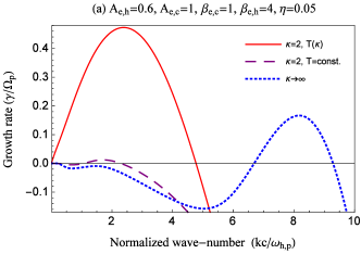
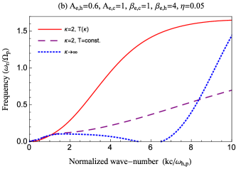
Figure 6: EFHI: growth rates (top) and real frequencies (bottom) derived for a dual model comprising a Maxwellian core and a bi-Kappa halo ($\kappa=2$) with $\kappa-$dependent temperatures (solid lines), $\kappa-$independent temperatures (dashed lines), or their bi-Maxwellian limit ($\kappa\to\infty$, dotted-lines). The plasma parameters for electrons are given explicitly in each panel and for protons are $A_{p,c}=A_{p,h}=1$, $\beta_{p,c}=1$, $\beta_{p,h}=4$.

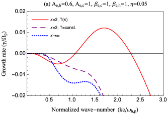
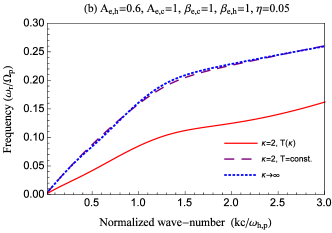
Figure 7: The same as in Fig. 6, but for a lower plasma beta $\beta_{e,h}=1$. The plasma parameters for electrons are given explicitly in each panel and for protons are $A_{p,c}=A_{p,h}=1$, $\beta_{p,c}=\beta_{p,h}=1$.

3 Kappa electrons: destabilizing effects

In this section we extend our comparative study to the effects of suprathermal (halo) electrons on the temperature anisotropy instabilities as they are predicted by the same dual Maxwellian-Kappa model when the temperatures of Kappa populations are dependent or independent of $\kappa$. Also considered is a comparison with the Maxwellian limit $\kappa\to\infty$ that enables us to emphasize the effects of suprathermal electrons which are expected to stimulate the instability.

According to the reports on the temperature anisotropy in the solar wind (Štverák et al., 2008; Pierrard et al., 2016) both the core and halo populations may exhibit anisotropies, and the halo is in general more anisotropic being hotter and less dense than the core. Therefore, in order to depict the effects of the suprathermal populations, here we minimize the influence of the Maxwellian core assuming isotropic with $T_{c,\parallel}=T_{c,\perp}=T_{c}$ (i.e., $A_{c}=T_{c,\perp}/T_{c,\parallel}=1$). In the solar wind the electron halo may exhibit both deviations from isotropy, namely, an excess of temperature in parallel direction $A_{e,h}<1$ that can drive the so-called electron firehose (EFH) instability, or an excess of temperature in perpendicular direction $A_{e,h}>1$ that can be at the origin of the whistler instability (WI), also known as the electromagnetic electron-cyclotron (EMEC) instability. We have analyzed the unstable solutions for a significant number of cases, keeping constant the core parameters for average values measured in the solar wind, e.g., $A_{e,c}=1$, $\beta_{e,c}=1$ the relative halo-core density $\eta=0.05$, and varying the halo parameters, i.e., $A_{e,h}$, $\beta_{e,h}$, and $\kappa$.

3.1 Firehose instability

We first discuss the electron firehose instability (EFHI) which is driven by a temperature anisotropy $A_{e,h}=T_{h,\perp}/T_{h,\parallel}<1$ of the electron halo component. The contribution of protons is minimized by considering them isotropic (both the proton core and halo components), such that the dispersion relation for the EFHI can take the following form

$$\tilde{k}^{2}=\mu\left[A_{e,h}-1+\dfrac{A_{e,h}\left(\tilde{\omega}+\mu\right)-\mu}{\tilde{k}\sqrt{\alpha^{2}\;\mu\;\beta_{e,h}^{\;\kappa}}}Z_{\kappa}\left(\frac{\tilde{\omega}+\mu}{\tilde{k}\sqrt{\alpha^{2}\;\mu\;\beta_{e,h}^{\;\kappa}}}\right)\right]$$ (18)

$$+\dfrac{1}{\eta}\left[\dfrac{\tilde{\omega}}{\tilde{k}\sqrt{\eta\;\beta_{p,c}}}Z_{M}\left(\frac{\tilde{\omega}-1}{\tilde{k}\sqrt{\eta\;\beta_{p,c}}}\right)\right]+\dfrac{\tilde{\omega}}{\tilde{k}\sqrt{\alpha^{2}\;\beta_{p,h}^{\;\kappa}}}Z_{\kappa}\left(\frac{\tilde{\omega}-1}{\tilde{k}\sqrt{\alpha^{2}\;\beta_{p,h}^{\;\kappa}}}\right)$$

$$+\dfrac{\mu}{\eta}\left[\dfrac{\tilde{\omega}}{\tilde{k}\sqrt{\mu\;\eta\;\beta_{e,c}}}Z_{M}\left(\frac{\tilde{\omega}+\mu}{\tilde{k}\sqrt{\mu\;\eta\;\beta_{e,c}}}\right)\right]$$

where $\tilde{k}=\leavevmode\nobreak\ kc/\omega_{h,p}$, $\tilde{\omega}=\omega/\Omega_{p}$, $\kappa=\leavevmode\nobreak\ \kappa_{e,p}$, $\alpha=(1-1.5/\kappa)^{0.5}$, $\mu=\leavevmode\nobreak\ m_{p}/m_{e}$ is the proton-electron mass ratio, $\eta$ is the halo-core relative density, $A_{j,h}$, $A_{j,c}$, respectively, are, respectively, the halo and core temperature anisotropies for protons (subscript $j=p$) or electrons (subscript $j=e$), $\beta_{j,h}^{\;\kappa}=8\pi nk_{B}T_{j,h,\parallel}/B_{0}^{2}$ and $\beta_{j,c}=8\pi nk_{B}T_{j,c,\parallel}/B_{0}^{2}$ are the plasma beta parameters for different plasma components, $Z_{j,M}$ is the standard dispersion function for (bi)-Maxwellian distributed plasmas, and $Z_{j,\kappa}$ is the modified dispersion function for (bi)-Kappa distributed plasmas (see Appendix A for the definitions of these functions).

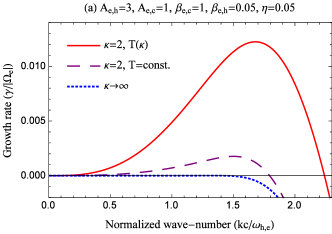
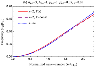
Figure 8: WI: growth rates (top) and real frequencies (bottom) derived for a dual model comprising a Maxwellian core and a bi-Kappa halo ($\kappa=2$) with $\kappa-$dependent temperatures (solid lines), $\kappa-$independent temperatures (dashed lines), or their bi-Maxwellian limit ($\kappa\to\infty$, dotted-lines). The electron plasma parameters are given explicitly in each panel.

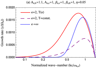
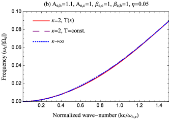
Figure 9: The same as in Fig. 8, but for a lower halo anisotropy $A_{e,h}=\leavevmode\nobreak\ 1.1$, and a higher plasma beta $\beta_{e,h}=1$.

Since the plasma beta parameter is an important factor in triggering the EFH instability by the anisotropic electrons with $A_{e}<1$, the unstable solutions displayed in Figs. 6 and 7 are derived for two distinct conditions, respectively, for a high halo plasma beta $\beta_{e,h}=4$, and for a lower $\beta_{e,h}=1$. For each of these two cases, the comparison invokes both Kappa approaches ($\kappa=2$) with temperatures dependent or independent of $\kappa$, as well as their Maxwellian limit ($\kappa\to\infty$). The growth rates (top panels) predicted by a Kappa model with $\kappa-$dependent temperatures are markedly enhanced in the presence of suprathermals. For instance, in Fig. 7 only this model predicts an instability, while the system becomes stable within the other two approaches. A systematic stimulation of the EFH instability in the presence of suprathermal electrons is confirmed only by a Kappa model with $\kappa-$dependent temperatures. The corresponding wave-frequencies (bottom panels) also show distinct and important variations with the Kappa models and the power-index $\kappa$.

3.2 Electron cyclotron (whistler) instability

In the opposite case an excess of perpendicular temperature $A_{e,h}=T_{h,\perp}/T_{h,\parallel}>1$ may drive the whistler instability. Since the wave frequency of the whistler modes is high ($\omega\gg\Omega_{p}$), the protons do not react and the dispersion relation that describes the whistler instability (WI) in a dual Maxwellian-Kappa plasma reads (Lazar et al., 2015b)

$$K^{2}=A_{e,h}-1+\dfrac{A_{e,h}\left(W-1\right)+1}{\tilde{k}\sqrt{\alpha^{2}\;\beta_{e,h}^{\;\kappa}}}Z_{\kappa}\left(\frac{W-1}{K\sqrt{\alpha^{2}\;\beta_{e,h}^{\;\kappa}}}\right)$$ (19)

$$+\dfrac{1}{\eta}\left[\dfrac{W}{K\sqrt{\eta\;\beta_{e,c}}}Z_{M}\left(\frac{W-1}{K\sqrt{\eta\;\beta_{e,c}}}\right)\right]$$

where $K=kc/\omega_{h,e}$, $W=\omega/|\Omega_{e}|$, and the other quantities are the same as explained above for the EFHI.

Figs. 8 and 9 present two representative conditions for the WI, respectively, when the halo plasma beta is low $\beta_{e,h}=0.05$ but the halo anisotropy is high $A_{e,h}=3$, and for a higher $\beta_{e,h}=1$ and a low anisotropy $A_{e,h}=1.1$. For even higher betas the instability can be triggered by very low anisotropies close to the isotropy condition $A_{e,h}\to 1$. Top panels display the growth-rates, and the corresponding wave-frequencies are plotted in the bottom panels. The unstable solutions are derived for both Kappa approaches ($\kappa=2$), with temperatures dependent or independent of $\kappa$, and for their Maxwellian limit ($\kappa\to\infty$) enabling us to emphasize the effects of suprathermal populations. Comparing the growth rates from different models, a systematic stimulation of the instability in the presence of suprathermals can be inferred only for the approach with $\kappa$-dependent temperatures. The other Kappa approach assuming $\kappa$-independent temperature leads to an irregular variation of the growth rates with $\kappa$. Unlike the growth-rates, the wave frequencies are not markedly influenced by the Kappa models and the variation of $\kappa$.

4 Conclusions

The temperature and power-index $\kappa$ are the main fitting parameters in a Kappa distribution model widely invoked to describe the velocity distributions of plasma particles and their dynamics. Recent studies have raised an important question on two alternative approaches, considering the temperature of Kappa populations either dependent or independent of $\kappa$. Various scenarios can provide justification for each of these two approaches, but observational evidences supporting any of them are not reported yet. Here we have shown for the first time that Kappa populations observed in the solar wind exhibit a direct interdependence between $T$ and $\kappa$. Thus, the temperature decreases with increasing $\kappa$

$$T_{\kappa}={\kappa\over\kappa-3/2}T_{\kappa\to\infty},$$ (20)

converging asymptotically to a limit that can be considered the cooler Maxwellian limit $T_{\kappa\to\infty}=T_{M}^{(}a)$, defined (by the components) in Eqs. (12)-(13). This is exactly the variation predicted by the previous studies (Lazar et al., 2015a, 2016a; Pierrard et al., 2016). It is important to emphasize that observational data invoked in the present paper are obtained with a refined dual Maxwellia-Kappa model, which is more accurate than a global Kappa in reproducing the observed distributions and implicitly the Kappa populations. We have also used these two approaches with temperatures dependent or independent of $\kappa$ to describe and compare the effects of suprathermal electrons on two electromagnetic instabilities driven by the temperature anisotropy, namely, the firehose and whistler instabilities. Only the approach with $\kappa$-dependent temperatures may confirm the expectation predicting a systematic stimulation of the instabilities by increasing the presence of suprathermals, while a Kappa approach with constant temperatures leads to a questionable variation of the growth rates with $\kappa$.

Appendix A: Plasma dispersion functions

For the bi-Maxwellian distributed plasma components (e.g., the core of different species, i.e., electrons with subscript $j=e$ and protons with subscript $j=p$), the plasma dispersion function in Eqs. (18) and (19) takes the standard form (Fried & Conte, 1961)

$$Z_{j,M}\left(\xi_{j,M}^{\pm}\right)=\frac{1}{\pi^{1/2}}\int_{-\infty}^{\infty}\frac{\exp\left(-x^{2}\right)}{x-\xi_{j,M}^{\pm}}dt,\ \ \Im\left(\xi_{j,M}^{\pm}\right)>0$$ (21)

of argument $\;\xi_{j,M}^{\pm}=\left(\omega\pm\Omega_{j}\right)/\left(k\;\theta_{j,\parallel,}\right)$. For the bi-Kappa distributed components, in the dispersion relations (18) and (19) we use the modified Kappa dispersion function (Lazar et al., 2008)

$$Z_{j,\kappa}\left(\xi_{j,\kappa}^{\pm}\right) =\frac{1}{\pi^{1/2}\kappa^{1/2}}\frac{\Gamma\left(\kappa\right)}{\Gamma\left(\kappa-1/2\right)}$$ (22)

$$\times\int_{-\infty}^{\infty}\frac{\left(1+x^{2}/\kappa\right)^{-\kappa}}{x-\xi_{j,\kappa}^{\pm}}dx,\ \Im\left(\xi_{j,\kappa}^{\pm}\right)>0,$$

of argument $\;\xi_{j,\kappa}^{\pm}=\left(\omega\pm\Omega_{j}\right)/\left(k\;\theta_{j,\parallel,}\right).$ In these equations $\pm$ denote the circular polarizations, right-handed (RH) and left-handed (LH), respectively, and $\Omega_{j}$ is the (non-relativistic) gyrofrequency.

References

- Christon et al. (1989) Christon, S. P., Williams, D. J., Mitchell, D. G., Frank, L. A., & Huang, C. Y. 1989, J. Geophys. Res., 94, 13409
- Collier et al. (1996) Collier, M. R., Hamilton, D. C., Gloeckler, G., Bochsler, P., & Sheldon, R. B. 1996, Geochim. Res. Lett., 23, 1191
- Feldman et al. (1975) Feldman, W. C., Asbridge, J. R., Bame, S. J., Montgomery, M. D., & Gary, S. P. 1975, J. Geophys. Res., 80, 4181
- Fried & Conte (1961) Fried, B. D. & Conte, S. D. 1961, The plasma dispersion function: the Hilbert transform of the Gaussian
- Gary et al. (1975) Gary, S. P., Feldman, W. C., Forslund, D. W., & Montgomery, M. D. 1975, J. Geophys. Res., 80, 4197
- Gary et al. (1994) Gary, S. P., Moldwin, M. B., Thomsen, M. F., Winske, D., & McComas, D. J. 1994, J. Geophys. Res., 99, 23
- Hellberg et al. (2005) Hellberg, M., Mace, R., & Cattaert, T. 2005, Space Sci. Rev., 121, 127
- Lazar et al. (2016a) Lazar, M., Fichtner, H., & Yoon, P. H. 2016a, A&A, 589, A39
- Lazar et al. (2015a) Lazar, M., Poedts, S., & Fichtner, H. 2015a, A&A, 582, A124
- Lazar et al. (2014) Lazar, M., Poedts, S., & Schlickeiser, R. 2014, Journal of Geophysical Research (Space Physics), 119, 9395
- Lazar et al. (2015b) Lazar, M., Poedts, S., Schlickeiser, R., & Dumitrache, C. 2015b, MNRAS, 446, 3022
- Lazar et al. (2008) Lazar, M., Schlickeiser, R., & Shukla, P. K. 2008, Physics of Plasmas, 15, 042103
- Lazar et al. (2016b) Lazar, M., Shaaban, S. M., Poedts, S., & Štverák, Š. 2016b, MNRAS
- Leubner (2004) Leubner, M. P. 2004, ApJ, 604, 469
- Livadiotis & McComas (2013) Livadiotis, G. & McComas, D. J. 2013, Space Sci. Rev., 175, 183
- Maksimovic et al. (1997) Maksimovic, M., Pierrard, V., & Riley, P. 1997, Geochim. Res. Lett., 24, 1151
- Maksimovic et al. (2005) Maksimovic, M., Zouganelis, I., Chaufray, J.-Y., et al. 2005, Journal of Geophysical Research (Space Physics), 110, A09104
- Nieves-Chinchilla & Viñas (2008) Nieves-Chinchilla, T. & Viñas, A. F. 2008, Journal of Geophysical Research (Space Physics), 113, A02105
- Pierrard & Lazar (2010) Pierrard, V. & Lazar, M. 2010, Sol. Phys., 267, 153
- Pierrard et al. (2016) Pierrard, V., Lazar, M., Poedts, S., et al. 2016, Sol. Phys., 291, 2165
- Pierrard et al. (1999) Pierrard, V., Maksimovic, M., & Lemaire, J. 1999, J. Geophys. Res., 104, 17021
- Pilipp et al. (1987) Pilipp, W. G., Muehlhaeuser, K.-H., Miggenrieder, H., Montgomery, M. D., & Rosenbauer, H. 1987, J. Geophys. Res., 92, 1075
- Shaaban et al. (2016) Shaaban, S. M., Lazar, M., Poedts, S., & Elhanbaly, A. 2016, Journal of Geophysical Research: Space Physics, 121, 6031, 2016JA022587
- Summers & Thorne (1991) Summers, D. & Thorne, R. M. 1991, Physics of Fluids B, 3, 1835
- Štverák et al. (2008) Štverák, Š., Trávníček, P., Maksimovic, M., et al. 2008, Journal of Geophysical Research (Space Physics), 113, A03103
- Vasyliunas (1968) Vasyliunas, V. M. 1968, J. Geophys. Res., 73, 2839
- Viñas et al. (2010) Viñas, A., Gurgiolo, C., Nieves-Chinchilla, T., Gary, S. P., & Goldstein, M. L. 2010, Twelfth International Solar Wind Conference, 1216, 265
- Yoon (2014) Yoon, P. H. 2014, Journal of Geophysical Research (Space Physics), 119, 7074
- Zimbardo et al. (2010) Zimbardo, G., Greco, A., Sorriso-Valvo, L., et al. 2010, Space Sci. Rev., 156, 89