Trefoil knot structure during reconnection

Abstract

Three-dimensional images of evolving numerical trefoil vortex knots are used to study the growth and decay of the enstrophy and helicity. Negative helicity density ($h<0$) plays several roles. First, during anti-parallel reconnection, sheets of oppositely-signed helicity dissipation of equal magnitude on either side of the maximum of the enstrophy dissipation allow the global helicity ${\cal H}$ to be preserved through the first reconnection, as suggested theoretically (Laing et al.  2015) and observed experimentally (Scheeler et al.  2014). Next, to maintain the growth of the enstrophy and positive helicity within the trefoil while ${\cal H}$ is preserved, $h<0$ forms in the outer parts of the trefoil so long as the periodic boundaries do not interfere. To prevent that, the domain size $\ell$ is increased as the viscosity $\nu\to 0$. Combined, this allows two sets of trefoils to form a new scaling regime with linearly decreasing $(\sqrt{\nu}Z(t))^{-1/2}$ up to common $\nu$-independent times $t_{x}$ that the graphics show is when the first reconnection ends. During this phase there is good correspondence between the evolution of the simulated vortices and the reconnecting experimental trefoil of Kleckner and Irvine (2013) when time is scaled by their respective nonlinear timescales $t_{f}$. The timescales $t_{f}$ are based upon by the radii $r_{f}$ of the trefoils and their circulations $\Gamma$, so long as the strong camber of the experimental hydrofoil models is used to correct the published experimental circulations $\Gamma$ that use only the flat-plate approximation.

Even though most turbulent flows are neither homogeneous, isotropic or statistically steady, most of our undertanding of turbulence uses those assumptions. Part of the reason is that for both experiments and simulations it is difficult to inject unstable, inherently anisotropic configurations into flows. In particular, flows that are free of the effects of walls or periodicity. Kleckner and Irvine (2013) have shown how this can now be done experimentally by 3D-printing hydrofoil knots, either linked rings or trefoils, covering them with hydrogen bubbles, then yanking them out of a water tank. This creates helical vortex knots whose low pressure vortex cores are marked by strings of bubbles.

Scheeler et al. (2014) have extended this repertoire by showing how the trajectories of bubbles can be used to determine the evolution of their centreline helicities, a measure of topological helicity based upon how those trajectories cross one another from several perspectives. The advantage of determining the topology using this diagnostic is that it does not require direct measurements of the velocity $u$ and vorticity $\omega$ used by the continuum helicity density $h=\mbox{\boldmath$u$}\cdot\mbox{\boldmath$\omega$}$ (8). How the topology of bubble trajectories changes also provides a diagnostic for setting the timescales.

The surprising result for the evolution of the centreline helicity for the trefoil in Scheeler et al. (2014) is that this diagnostic is preserved despite clear signs that the topology of the trefoil is changing due to vortex reconnection. Would the true continuum helicity be preserved in numerical simulations that qualitatively reproduce the observed topological changes of the evolving experimental trefoils?

This paper will use two sets of high-resolution, strongly perturbed trefoils fromKerr (2017) to identify how physical space structures reconnect during a period for which the continuum global helicity ${\cal H}$ (8) is similarly preserved. Kerr (2017) also identified a new scaling regime for the growth of $\sqrt{\nu}Z(t)$, $\nu$ the viscosity and $Z$ the volume-integrated enstrophy (7), that was first indicated by $\nu$-independent crossing times $t_{x}$ with a common $\sqrt{\nu}Z(t_{x})$. What is the role of the structures in the dynamics responsible for this unexpected behaviour of both the helicity ${\cal H}$ and enstrophy $Z$ over this period? The plan is to use three-dimensional graphics from a time just before reconnection begins to the time, after reconnection ends, when helicity finally begins to decay to address that question.

The trefoils’ initial trajectories are illustrated in figure 1 and figure 2 summarises the $\sqrt{\nu}Z$ scaling using

$$B_{\nu}(t)=\Bigl{(}\sqrt{\nu}Z(t)\Bigr{)}^{-1/2}\quad{\rm with}~{}\nu{\rm-independent}\quad B_{x}=B_{\nu}(t_{x})\quad{\rm at}~{}t_{x}\,.$$ (1)

The characteristic crossing times are $t_{x}$(Q)=40 and $t_{x}$(S)$\approx$45 for the Q and S-trefoil calculations listed in table 1 and $B_{\nu}(t)$ is linearly decreasing in both subplots for $t_{\Gamma}\!\leq\!t\!\leq\!t_{x}$, $t_{\Gamma}\approx 15$. By linearly extrapolated this behaviour to critical times $T_{c}(\nu)>t_{x}$ using

$$T_{c}(\nu)=\frac{t_{x}-t_{\Gamma}B_{x/\Gamma}(\nu)}{1-B_{x/\Gamma}(\nu)}\quad{\rm where}\quad B_{x/\Gamma}(\nu)=B_{x}/B_{\nu}(t_{\Gamma})\,,$$ (2)

self-similar collapse was identified over the times $t_{\Gamma}\leq t\leq t_{x}$ (Kerr  2017) using

$$(T_{c}(\nu)-t_{x})\bigl{(}B_{\nu}(t)-B_{x}\bigr{)}=(T_{c}(\nu)-t_{x})\left(\Bigl{(}\sqrt{\nu}Z(t)\Bigr{)}^{-1/2}-B_{x}\right)\,.$$ (3)

Kerr (2017) also showed that this self-similar collapse could be applied to new anti-parallel calculations and provided three-dimensional graphics to show that the anti-parallel $t_{\Gamma}$ is when reconnection began by exchanging circulation $\Gamma$ between the vortices and that the $t_{x}$ determined by the crossings of $B_{\nu}(t)$ is when those reconnections finish. It will be shown in section 3.2 that $t_{x}$(Q)=40 also represents the end of the first Q-trefoil reconnection and is the best timescale for comparisons with the experiments of Kleckner and Irvine (2013).

The comparisons between the Q-trefoil images and those from Kleckner and Irvine (2013) are feasible because the perturbed trefoils, illustrated in figure 1, were constructed so that there would be a single dominant initial reconnection, as in the experiments, with the comparisons around the reconnection time $t\sim t_{x}$ discussed in section 3.2. Establishing those similarities justifies using the simulations to provide diagnostics that are inaccessible to those experiments, but needed for explaining the observed dynamics. For example, figure 6 shows the terms in helicity budget equation (8) that might allow preservation of the global helicity.

How do the global helicity ${\cal H}(t)$ and energy dissipation rate $\epsilon(t)=\nu Z$ (6) evolve after $t=t_{x}$? For both trefoils and before $t\sim 2t_{x}$, ${\cal H}(t)$ begins to decay in figure 3 and for the dissipation rate, figure 2 indicates fixed times $t_{\epsilon}$ (stars) when the $\nu$-independent dissipation rates $\epsilon(t)$ start to saturate for $t>t_{\epsilon}$. The constant $\epsilon(t_{\epsilon})=\nu Z(t_{\epsilon})$ and earlier constant $\sqrt{\nu}Z(t_{x})$ both imply that $Z\!\to\!\infty$ as $\nu\!\to\!0$. Can this growth in the enstrophy $Z$ be maintained as $\nu\!\to\!0$, eventually leading to a dissipation anomaly? That is, can there be finite energy dissipation in a finite time as $\nu\!\to\!0$?

To answer that, Kerr (2017) considered the effect of accepted Sobolev space mathematical analysis for smooth solutions of the Navier-Stokes equation that shows that if the domain size $V=\ell^{3}$ is fixed, then $Z(t)$ has an upper bound as $\nu\!\to\!0$ (Constantin  1986). However, this mathematics also allows this constraint to be relaxed by increasing $\ell$. This escape valve, increasing the domain size $V=\ell^{3}$ as $\nu\!\to\!0$, was used for both the trefoils and the anti-parallel vortices to ensure that the collapse defined by (3) could be maintained as the viscosity $\nu$ was decreased. Is there physical space dynamics that underlies this rigorously derived constraint and its relaxation? The late time graphics in section 3.4 will suggest that these effects could arise from the generation of negative helicity in the outer parts of the trefoil domain.

The thinner-core S-trefoils have been included to provide continuum helicity ${\cal H}$ comparisons to the centreline helicity diagnostics of the thinner vortex core trefoil experiment of Scheeler et al. (2014), which Kleckner and Irvine (2013) did not provide. The connection to the physical space diagnostics from Kleckner and Irvine (2013) will be provided by the similarities between the Q and S-trefoils for the evolution of $B_{\nu}(t)$ (1) and global helicity (8) in figures 2 and 3.

This paper is organised as follows. After introducing the equations, diagnostics and initialisation, illustrated for the Q-trefoil in figure 1, there is a short review of the $\sqrt{\nu}Z$ enstrophy scaling results in Kerr (2017). Then a re-evaluation of the circulations reported for the experiments and the new timescales these imply. Once these are established, then graphics and analysis connecting the dynamics of positive helicity and enstrophy production and the appearance of negative helicity increasingly far from the original trefoil will be given. At the end, structural changes during the last period when helicity finally begins to decay and finite energy dissipation is generated are presented.

1 Equations, diagnostics and initial condition

The governing equations in this paper will be the incompressible Navier-Stokes velocity equations

$$\frac{\partial\mbox{\boldmath$u$}}{\partial t}+({\mbox{\boldmath$u$}}\cdot\nabla){\mbox{\boldmath$u$}}=-\nabla p+\underbrace{\nu\triangle{\mbox{\boldmath$u$}}}_{\rm dissipation},\qquad\nabla\cdot{\mbox{\boldmath$u$}}=0$$ (4)

and the diagnostics will primarily use the vorticity $\mbox{\boldmath$\omega$}=\nabla\times\mbox{\boldmath$u$}$ , which obeys

$$\frac{\partial\mbox{\boldmath$\omega$}}{\partial t}+({\mbox{\boldmath$u$}}\cdot\nabla){\mbox{\boldmath$\omega$}}=({\mbox{\boldmath$\omega$}}\cdot\nabla){\mbox{\boldmath$u$}}+\nu\triangle{\mbox{\boldmath$\omega$}},\qquad\nabla\cdot{\mbox{\boldmath$\omega$}}=0\,.$$ (5)

All of the calculations were done in periodic boxes of variable size ($V=\ell^{3}$). The continuum equations for the densities of the energy, enstrophy and helicity, $e=\mbox{$\frac{1}{2}$}|\mbox{\boldmath$u$}|^{2}$, $|\mbox{\boldmath$\omega$}|^{2}$ and $h=\mbox{\boldmath$u$}\cdot\mbox{\boldmath$\omega$}$ respectively are (with their volume-integrated measures):

$$\frac{\partial e}{\partial t}+({\mbox{\boldmath$u$}}\cdot\nabla)e=-\nabla\cdot(\mbox{\boldmath$u$}p)+\nu\triangle e-\underbrace{\nu(\nabla\mbox{\boldmath$u$})^{2}}_{\epsilon={\rm dissipation}=\nu Z},\qquad E=\mbox{$\frac{1}{2}$}\int\mbox{\boldmath$u$}^{2}dV\,.$$ (6)

$$\frac{\partial|\mbox{\boldmath$\omega$}|^{2}}{\partial t}+({\mbox{\boldmath$u$}}\cdot\nabla)|\mbox{\boldmath$\omega$}|^{2}=\underbrace{2\mbox{\boldmath$\omega$}\mbox{\boldmath$S$}\mbox{\boldmath$\omega$}}_{Z_{p}={\rm production}}+\nu\triangle|\mbox{\boldmath$\omega$}|^{2}-\underbrace{2\nu(\nabla\mbox{\boldmath$\omega$})^{2}}_{\epsilon_{\omega}=Z-{\rm dissipation}},\qquad Z=\int\mbox{\boldmath$\omega$}^{2}dV\,.$$ (7)

$$\frac{\partial h}{\partial t}+({\mbox{\boldmath$u$}}\cdot\nabla)h=\underbrace{-\mbox{\boldmath$\omega$}\cdot\nabla\Pi}_{\omega-{\rm transport}}+\underbrace{\nu\mbox{\boldmath$\triangle$}h}_{\nu-{\rm transport}}-\underbrace{2\nu{\rm tr}(\nabla\mbox{\boldmath$\omega$}\cdot\nabla\mbox{\boldmath$u$}^{T})}_{\epsilon_{h}={\cal H}-{\rm dissipation}}\qquad{\cal H}=\int\mbox{\boldmath$u$}\cdot\mbox{\boldmath$\omega$}dV\,.$$ (8)

$\Pi=p-\mbox{$\frac{1}{2}$}\mbox{\boldmath$u$}^{2}\neq p_{h}$ is not the pressure head $p_{h}=p+\mbox{$\frac{1}{2}$}\mbox{\boldmath$u$}^{2}$. Both the global energy $E$ and helicity ${\cal H}$ are inviscid invariants, but the local helicity density $h$ is not locally Galilean invariant due to the $\omega$-transport term and its role in nonlinearity is not fully understood (Moffatt  2014). The global helicity ${\cal H}$ has same dimensional units as the circulation-squared.

The circulations $\Gamma_{i}$ about vortices with distinct trajectories $\mbox{\boldmath$x$}_{i}\in{\cal C}_{i}$ are another set of inviscid invariants:

$$\Gamma_{i}=\oint\mbox{\boldmath$u$}_{i}\cdot d\mbox{\boldmath$r$}_{i}\quad{\rm where}\quad\mbox{\boldmath$r$}_{i}~{}~{}\mbox{is a closed loop about}~{}~{}{\cal C}_{i}\,.$$ (9)

Under Navier-Stokes dynamics, these circulations will change as vortices of opposite sign meet and begin to reconnect in a gradual process where, through the viscous terms, new vortices are generated as the original vortices annihilate one another, as demonstrated by figure 5.

Under Navier-Stokes dynamics, the local helicity density can be of either sign, can grow, decrease and even change sign due to both the viscous terms and the $\omega$-transport term along the vortices in (8). Also, unlike the kinetic energy which cascades overwhelmingly to small scales, $h$ can move to both large and small scales (Biferale and Kerr 1995, Sahoo et al. 2015).

The diagnostics will be continuum properties in the equations above (6,7,8) and a few discrete vortex trajectories (11). Of these, the most important vorticity diagnostic will be the enstrophy $Z$, which can grow inviscidly due to its production term $Z_{p}$. The maximum of vorticity magnitude will be denoted

$$\|{\omega}\|_{\infty}=\sup|\mbox{\boldmath$\omega$}|$$ (10)

and its location $\mbox{\boldmath$x$}_{\infty}$ will be used to seed the trajectories of vortex lines. However, $\|\omega\|_{\infty}$ will not have its usual Hölder significance as a volume-averaged upper bound for all norms because $Z$ and ${\cal H}$ will be volume-integrated norms,

1.1 Vortex lines and linking numbers

To provide qualitative comparisons with the experimental vortex lines (Kleckner and Irvine 2013, Scheeler et al. 2014), vortex lines $\mbox{\boldmath$x$}_{j}(s)$ were identified by solving the following ordinary differential equation using the Matlab streamline function,

$$\frac{d\mbox{\boldmath$x$}_{j}(s)}{ds}=\mbox{\boldmath$\omega$}(\mbox{\boldmath$x$}_{j}(s))\,.$$ (11)

The seeds for solving (11) were chosen from the positions around, but not necessarily at, local vorticity maxima.

When the vortices are distinct with closed trajectories, these vortex lines have the following topological numbers: The integer linking numbers ${\cal L}_{ij}$ between all distinct vortex trajectories, the integer self-linking numbers ${\cal L}_{Si}=W\!r_{i}+T\!w_{i}$ of individual closed loops, and the non-integer writhe and twist $W\!r_{i}$ and $T\!w_{i}$. Then, by assigning circulations $\Gamma_{i}$ to the vortices and summing one can determine the global helicity ${\cal H}$ (Moffatt and Ricca  1992).

$${\cal H}=\sum_{ij}\Gamma_{i}\Gamma_{j}{\cal L}_{ij}+\sum_{i}\Gamma_{i}^{2}{\cal L}_{S_{i}}\,.$$ (12)

The quantitative tool that is used to determine the writhe, self-linking and intervortex linking numbers in figure 5 is a regularised Gauss linking integral about two loops $\mbox{\boldmath$x$}_{i}\in{\cal C}_{i}$ and $\mbox{\boldmath$x$}_{j}\in{\cal C}_{j}$

$${\cal L}_{ij}=\sum_{ij}\frac{1}{4\pi}\oint_{{\cal C}_{i}}\oint_{{\cal C}_{j}}\frac{(d\mbox{\boldmath$x$}_{i}\times d\mbox{\boldmath$x$}_{j})\cdot(\mbox{\boldmath$x$}_{i}-\mbox{\boldmath$x$}_{j})}{(|\mbox{\boldmath$x$}_{i}-\mbox{\boldmath$x$}_{j}|^{2}+\delta^{2})^{1.5}}\,.$$ (13)

The regularisation of the denominator using $\delta$ has been added for determining the writhe when $i=j$ (Calugareanu 1959,Moffatt and Ricca 1992), with $\delta\equiv 0$ for directly determining the self-linking numbers ${\cal L}_{Si}$ using two parallel trajectories within the vortex cores, as illustrated in figure 1, and for the intervortex linking numbers with $i\neq j$

Defining the Frenet-Serret relations of a curve in space: $\mbox{\boldmath$x$}(s):[0,1]\rightarrow\mathbb{R}^{3}$ as

$$\mbox{\boldmath$T$}(s)=\partial_{s}\mbox{\boldmath$x$}_{j}(s);\quad\partial_{s}\mbox{\boldmath$N$}=\tau\mbox{\boldmath$B$}-\kappa\mbox{\boldmath$T$};\quad\kappa\mbox{\boldmath$N$}=\partial_{s}\mbox{\boldmath$T$};\quad\partial_{s}\mbox{\boldmath$B$}=-\tau\mbox{\boldmath$N$}\,,$$ (14)

where the $\kappa$ is the curvature and $\tau$ is the torsion, the intrinsic twist of a closed loop $T\!w_{i}$ can in principle be determined from the line integral of the torsion of the vortex lines:

$$T\!w_{i}=\frac{1}{2\pi}\oint\tau ds,\qquad{\rm where}\quad\tau=\frac{d\mbox{\boldmath$N$}}{ds}\cdot\mbox{\boldmath$B$}\,.$$ (15)

Because determining $\tau$ requires taking third-derivatives of the positions $\mbox{\boldmath$x$}(s)$, which the single-precision analysis data used here cannot determine accurately, the values of the twist will always be $T\!w={\cal L}_{S}-W\!r$.

Figure 1: Vorticity isosurface plus two closed vortex lines of the perturbed trefoil vortex at $t=6$, not long after initialization. Its self-linking is ${\cal L}_{S}=3$, which can be split into writhe of $W\!r=3.15$ and twist of $T\!w=-0.15$.

Cases	Domains	$r_{0}$	$\omega_{\rm in}$	$k_{f}$	$r_{e}$	$\omega_{0}$	$Z_{0}$	$E_{0}$	$\nu$
Q	$(3\pi)^{3}$	0.25	1.26	11.9	0.40	1	$5.48$	0.96	5e-4 to 1.25e-4
Q	$(4\pi)^{3}$	0.25	1.26	11.9	0.40	1	$5.29$	0.85	$5\times 10^{-4}$ to $6.25\times 10^{-5}$
Q	$(6\pi)^{3}$	0.25	1.26	11.9	0.40	1	$5.30$	0.90	$3.125\times 10^{-5}$
S	$(6\pi)^{3}$	0.125	5	23.8	0.20	4	$17.7$	1.03	(2.5 and 1.25)$\times 10^{-4}$
S	$(9\pi)^{3}$	0.125	5	23.8	0.20	4	$17.8$	1.13-1.17	(6.25 and 3.125)$\times 10^{-5}$
S	$(12\pi)^{3}$	0.125	5	23.8	0.20	4	$17.8$	1.13-1.17	$7.8\times 10^{-6}$

Table 1: Parameters for the initial conditions using (17) and viscosities of the cases. $r_{0}$ and $\omega_{\rm in}$ are the pre-filter radius and vorticity of the filaments. $k_{f}$ are the filter wavenumbers that give initial conditions with $\omega_{0}=\|\mbox{\boldmath$\omega$}\|_{\infty}$, enstrophy=$Z_{0}$ and energy=$E_{0}$. The final meshes for the $(3\pi)^{3}$ calculations were $512^{3}$, for the $\nu\geq 1.25\times 10^{-4}$ $(4\pi)^{3}$ calculations were $1024^{3}$ and for the rest $2048^{3}$. The initial helicity for all of the calculations is ${\cal H}(t=0)=7.67\times 10^{-4}$ for circulations of $\Gamma=0.505$. The $(3\pi)^{3}$-Q cases are used only for graphics.

1.2 Initial condition and length scales

The initial trajectory of all of the simulated trefoils will be

$$\begin{array}[]{rrl}x(\phi)=r(\phi)\cos(\alpha)&\quad y(\phi)=&r(\phi)\sin(\alpha)\qquad z(\phi)=a\cos(\alpha)\\ {\rm where}&r(\phi)=&r_{f}+r_{1}a\cos(\phi)+a\sin(w\phi+\phi_{0})\\ {\rm and}&\alpha=&\phi+a\cos(w\phi+\phi_{0})/(wr_{f})\end{array}$$ (16)

with $r_{f}=2$, $a=0.5$, $w=1.5$, $\phi_{0}=0$, $r_{1}=0.25$ and $\phi=[1:4\pi]$. This weave winds itself twice about the central deformed ring with: $x_{c}^{2}(\phi)+y_{c}^{2}(\phi)=r_{c}^{2}(\phi)$, where $r_{c}(\phi)=r_{f}+r_{1}a\cos(\phi)$ for a $r_{1}\neq 0$ perturbation. The separation through the $r=r_{c}$ ring of the two loops of the trefoil is $\delta_{a}=2a=1$. Four additional low intensity vortex rings, two moving up in $z$ and two down, provided the perturbation that breaks the three-fold symmetry of the trefoil so that it has a single major initial reconnection like the experiments. Once all the trajectories are defined, vortices of finite radii $r_{0}$ are mapped from this trajectory onto the mesh using a profile function based upon the Rosenhead regularisation of a point vortex, then the fields on the mesh are smoothed with a hyperviscous filter, as described previously (Kerr 2013, Kerr 2017).

$$|\omega_{i}|(r)=\Gamma\frac{(r_{0}^{2})}{(r^{2}+r_{0}^{2})^{2}},\quad\omega_{f}(\mbox{\boldmath$k$})=\omega_{i}(\mbox{\boldmath$k$})\exp\left(-\frac{k^{4}}{k_{f}^{4}}\right),\quad r_{e}=\left(\frac{\Gamma}{\omega_{0}/\pi}\right)^{1/2}$$ (17)

where the $r_{e}$ in table 1 are the radii of the smoothed vortices. All of the trefoils have a circulation of $\Gamma=0.505$ and after filtering their effective radii all obey $r_{e}\approx 1.6r_{0}$.

The two relevant length scales are $r_{f}=2$, the trefoil’s radius, and $r_{e}$, the effective thickness of the filaments. Two $r_{e}$ are listed in table 1, designated Q and S, with $r_{e}(S)=0.5r_{e}(Q)$, so that the effective cross-sectional areas of the vortices, $A(r_{e})=\pi r_{e}^{2}$, are $A(r_{e}(S))=\pi r_{e}^{2}(S)=0.25A(r_{e}(Q))=0.25\pi r_{e}^{2}(Q)$. To keep the circulations $\Gamma$ constant, the initial centreline vorticity $\|\omega\|_{\infty}(t=0)$ changes inversely with the $A(r_{e})$.

Figure 2: Scaling of $B_{\nu}(t)=(\sqrt{\nu}Z(t))^{-1/2}$ (1), inverse, $\sqrt{\nu}$-scaled enstrophies with $r_{e}$ dependent crossing times $t_{x}$ for the cases in table 1. Colours for the different viscosities are the same as in figure 3 Consistent decreasing $B_{\nu}(t)$ begins at $t_{\Gamma}\approx 15$ in each subplot and the dashed lines indicate the linear extrapolations that determine the effective critical times $T_{c}(\nu)$ (2). The $*$’s indicate when the energy dissipation rates $\epsilon=\nu Z$ begin to saturate at $\nu$-independent values of $\epsilon$. a: Q-trefoils with $t_{x}\approx 40$ for viscosities that vary by decreasing factors of 2 from $\nu=5\times 10^{4}$ (black) to $\nu=$3.125e-5 (green). The linearly-decreasing behaviour of $B_{\nu}(t)$ begins at $t_{\Gamma}\approx 15$ as negative helicity, as shown in figure 4, first appears in the graphics. Kerr (2017) used these $T_{c}(\nu)$ in (3) to find a self-similar collapse of the $B_{\nu}(t)$. b: S-trefoils with $t_{x}\approx 45$. The viscosities are those in figure 3 plus $\nu=2.5\times 10^{-4}$ and $6.125\times 10^{-5}$. $t_{\Gamma}=25$ was used for the $T_{c}(\nu)$ linear extrapolations.

Figure 3: Time evolution of the scaled helicity ${\cal H}^{1/2}$. In the main frame are 5 viscosities from $\nu=5\times 10^{-4}$ to $3.125\times 10^{-5}$ for the Q-cases. Important times during the evolution of the trefoil: The blue-$\square$ line is $t=31$, the time when the first signs of reconnection are visible as in figure 5. The dashed line is $t_{x}=40$, the time when all the $\sqrt{\nu}Z$ meet and the first reconnection ends. The brown-$\star$ line is $t_{Setal}=52$, roughly the equivalent time to when the Scheeler et al. (2014) experiment would end with respect to choosing $t_{x}(SK)=638$ms. The red-dot-dash line is the Q-trefoil dissipation saturation time $t_{\epsilon}=93$ indicated in figure 2. The upper-right inset shows ${\cal H}^{1/2}$ for three viscosities of the thinner core S-trefoils to show that the timescale for helicity decay is independent of the core thicknesses $r_{e}$.

2 Enstrophy evolution and timescales

Several nonlinear and viscous timescales can be applied to the vortex reconnection events. The most important nonlinear timescale for the numerical trefoils is identified in figure 2 by the viscosity-independent crossing time of $B_{\nu}(t)=(\sqrt{\nu}Z(t))^{-1/2}$ (1) at $t=t_{x}\approx 40$ for the Q-trefoils and $t_{x}\approx 45$ for the S-trefoils, indicating that $t_{x}$ is independent of $\nu$ and approximately independent of $r_{e}$. Figure 7 at $t=42$, discussed in section 3.2, demonstrates that $t_{x}\approx 40$ represents when the first reconnection ends in physical space for the Q-trefoils.

Nonlinear time and velocity scales that do not depend upon $\nu$ and $r_{e}$ can be formed using the circulation $\Gamma$ and the size of the structure $r_{f}$:

$$t_{f}=r_{f}^{2}/\Gamma\quad{\rm and}\quad v_{f}=\Gamma/r_{f}\,.$$ (18)

For both the Q and S-trefoils, $t_{f}$(Q)=$t_{f}$(S)$=2^{2}/0.5=8$ and $v_{f}=0.25$. Kerr (2017) concluded that $t_{f}=8$ and $t_{x}\approx 40$ are related, despite $t_{x}\sim 5t_{f}$, by finding the self-similar collapse (3) that covers the linearly decreasing regimes of $B_{\nu}(t)$ in figure 2.

For velocities, the nearly vertical maximum velocity is approximately $v_{f}$ and up to $t=20$ the vertical velocity of $\mbox{\boldmath$x$}_{\infty}$, the position of $\|\omega\|_{\infty}$, is $v_{\infty}\approx 0.25=v_{f}$. This is discussed further in section 3.2.

2.1 Experimental timesscales

How can equivalent reconnection times $t_{x}$ for the experiments of Kleckner and Irvine (2013) and Scheeler et al. ( 2013) be determined? Two routes for estimating the experimental reconnection timescales are considered. First, the experimental nonlinear timescale $t_{f}$ (18) can be estimated if $\Gamma$, the circulation of the shed vortex, and $r_{f}$, the radius of the knot (16), are known. Second, visual validation from the experimental reconnection figures, based upon when the first major reconnection has completed. There are problems with both approaches, so the $r_{f}=45$mm case from Kleckner and Irvine (2013) is discussed first because the timescales of both methods can be estimated from the available data and figures.

The problems are these. In the estimate of the experimental nonlinear timescale $t_{f}$ (18), the published circulations $\Gamma$ were not measured, but were estimated based upon a flat-plate approximation of

$$\Gamma_{\mbox{fp}}=\pi\mbox{UC}\sin\alpha\,.$$ (19)

The basic parameters that determine $\Gamma_{\rm fp}$ are C, the chord (width) of the hydrofoil, U, the velocity of the hydrofoil and the tilt $\alpha$ of the overall hydrofoil with respect to the direction of propagation. However, this neglects the contribution due to for the highly curved ribbons used in their 3D-printed knot models. In aeronautics this is known as the camber and is discussed in the next section.

The problem with defining $t_{x}$ as when the first reconnection ends using three-dimensional images is that this small, but significant, change in the topology cannot be identified from a single image in isolation, which can be interpreted in several ways. So multiple times need to be compared before a convincing, visually determined value for $t_{x}$ can be obtained. The strategy for addressing this problem will be to identify when a clear and persistent gap appears in the global trefoil structure. Then look backwards in time to the first earlier incident when along the trefoil vortex, there is a sudden local dispersion of the bubbles as lines meet and choose this as $t_{x}$. In figure 8, the clear gap is at $t=400$ms, and the earlier bubble dispersion event is at $t=350$ms. This will be discussed further in section 3.2.

2.2 Camber correction

To maximise the experimental circulation of their vortex knots, the 3D-printed knot models that Kleckner and Irvine (2013) and Scheeler et al. ( 2014b) accelerated through their water tank used curved ribbons whose trailing edge was tilted $\theta=15^{\circ}=\pi/12$ rad. This corresponds to an angle of attack of $\alpha=\theta/2$. The strong curvature or camber can be approximated as

$$y(x)=h{\displaystyle\frac{x({\rm C}-x)}{t}}\quad{\rm with}\quad\frac{h}{C}\approx\frac{\theta}{8}\,.$$ (20)

If $x=({\rm C}/2)(1-\cos\phi)$ for $0\leq\phi\leq\pi$, the camber correction can then be approximated as $\Delta\Gamma=(\pi/2)\mbox{UC}\,{\rm A}_{1}$ where $A_{1}$ is determined by the following integral of the derivative $dy/dx$ of the camber line (Houghton and Carpenter  2003)

$${\rm A}_{1}=(2/\pi)\int_{0}^{\pi}(dy/dx)\cos\phi d\phi=(2/\pi)(4h/{\rm C})\int_{0}^{\pi}\cos^{2}\phi d\phi=(4h/{\rm C})$$

giving

$$\Delta\Gamma=(\pi/2)\mbox{UC}\,{\rm A}_{1}=2\pi(h/{\rm C}){\rm UC}\approx\pi\mbox{UC}(\pi/48)\,.$$ (21)

This represents a 50% increase in the circulation on top of the primary flat plate contribution of $\Gamma_{\mbox{fp}}=\pi\mbox{UC}\pi/24$ for $\alpha=\theta/2=\pi/24$ using (19). Together

$$\Gamma=\Gamma_{\mbox{fp}}+\Delta\Gamma=1.5\Gamma_{\mbox{fp}}=\pi^{2}\mbox{UC}/16\,.$$ (22)

Once the camber-corrected $\Gamma$ are known, then the experimental nonlinear timescale $t_{f}$ (18) can be determined and its relationship with $t_{x}$ identified for comparisons with the simulations and the visible signs of experimental reconnection. What are the $t_{f}$ for the Kleckner and Irvine (2013) and Scheeler et al. (2014) experiments?

For the $r_{f}=45$mm experiment of Kleckner and Irvine (2013), with $U=3.1$m/s and the chord C=15mm, the circulation is $\Gamma=2.8\times 10^{4}$mm²/s (22) and the timescale is $t_{f}$(KI)=$r_{f}^{2}/\Gamma=70$ms (18). Based on the crossings of $B_{\nu}(t)$ at $t_{x}$ in figure 2a, the end of the first reconnection should be at $t_{x}$(KI)$=5t_{f}$(KI)=350ms, which would be consistent with the conclusion of Kleckner and Irvine (2013) and the discussion in section 3.2 using the $t=350$ms and $t=400$ms frames in figure 8 with reconnection gaps.

For Scheeler et al. (2014), (22) with $r_{f}=69$mm, C=22.5mm and U=2m/s, gives $t_{f}$(SK)=168ms. However, the predicted reconnection time of $=5t_{f}=840$ms is after the first clear gap at $t\!\approx$638ms$\ll$840ms. This will be discussed further in section 3.3.

Figure 4: Isosurfaces at $t=24$, shortly before reconnection begins. The vorticity isosurface is in blue, the position of $\|\mbox{\boldmath$\omega$}\|_{\infty}$ is X, the trefoil line through it is green and the helicity isosurfaces are: $0.06\max(h)$ in green and $0.2\min(h)$ in orange where $\max(h)=-0.22$ and $\min(h)=0.085$. The points with the minumum distance between the two loops of the trefoil, where reconnection is about to begin, are at the yellow and red +’s. At the red +, the trefoil is bending back upon itself to become anti-parallel to the yellow +. A kink is forming on the trefoil line to the left of $\|\mbox{\boldmath$\omega$}\|_{\infty}$ in another region of $h<0$.

Figure 5: A single vorticity isosurface plus three closed vortex lines at $t=31$, the first time that visible reconnection is observed. The green trajectory follows a trefoil trajectory seeded near $\|\mbox{\boldmath$\omega$}\|_{\infty}$ indicated by X. The green trajectory’s self-linking is ${\cal L}_{S}=4$, which can be split into $W\!r+T\!w=2.85+1.15=4$ At the closest approach of the trefoil’s two loops, due to an extra twist, the loops are anti-parallel, as indicated by two arrows. Between them is the reconnection zone whose mid-point is shown by the orange X. Trajectories seeded on either side of this point, away from the trefoil, become linked rings. For the red ring ${\cal L}_{S}=0$ and for the blue ${\cal L}_{S}=1$ with a total linking of ${\cal L}_{rb}+{\cal L}_{Sb}+{\cal L}_{Sr}=3$.

Figure 6: Multiple vorticity and dissipation isosurfaces at $t=36$ rotated 90^∘ clockwise from figure 5 at $t=31$. The black and red X’s mark the positions of $\|\omega\|_{\infty}$ and maximum enstrophy dissipation $\epsilon_{\omega-{\rm m}}=\max(\epsilon_{\omega})$ (7). The blue and yellow plus signs show the extremes of the helicity dissipation (8), $\epsilon_{{\rm h+}}=\max(\epsilon_{h})=4.9$ and $\epsilon_{{\rm h-}}=\min(\epsilon_{h})=-3.2$ respectively. The green vortex trajectory, a trefoil plus an extra loop, and the lower $\omega=0.33\|\omega\|_{\infty}$ cyan vorticity isosurface mostly follow the original trefoil. A gap exists in the green $\omega=0.53\|\omega\|_{\infty}$ vorticity isosurface in the reconnection zone between two red enstrophy dissipation isosurfaces with $\epsilon_{\omega}=0.5\epsilon_{\omega-{\rm m}}$. Around the black X at $\|\omega\|_{\infty}$ and stacked with the left $\epsilon_{\omega}$ red isosurface, are flattened isosurface of positive helicity dissipation, negative helicity dissipation and the advection of negative helicity, respectively as blue for $\epsilon_{h}=0.5\epsilon_{h+}$, yellow-orange for $\epsilon_{h}=0.5\epsilon_{h-}$ and magenta for transport of negative helicity $\mbox{\boldmath$u$}\cdot\nabla h=0.5\max(\mbox{\boldmath$u$}\cdot\nabla h)$ that will be tied to the later $t>t_{x}$, $h<0$ regions discussed in section 3.4.

3 Evolution of the topology of the initial reconnection

The purpose of this section is to outline and compare the structural changes during and after the first reconnection using three-dimensional numerical images from six times and experimental images at five times from Kleckner and Irvine (2013) in figure 8. The common graphical tools for all times will be at least one level of vorticity isosurfaces and one vortex line. Additional isosurfaces of the dissipation of enstrophy, both signs of helicity, both signs of helicity dissipation and the helicity transport will be added to the figures where appropriate.

For completeness and later analysis, the discussion will begin with figure 4 at $t=24$ to see what underlies the self-similar collapse that goes back to $t_{\Gamma}\approx 15$, as implied by figure 2, and to see the evolution of the twists that set up the first visible reconnection at $t=31$ in figure 5.

Figure 6 at $t=36$ shows the dynamical terms during reconnection, whose locations are compared with figures 7 and 9 at $t=42$ and 45 to show that the $t=t_{x}\approx 40$ crossing of $B_{\nu}(t)=(\sqrt{\nu}Z(t))^{-1/2}$ (1) in figure 2a is when the first reconnection ends with the formation of complete gaps in the trefoil structure, as Kerr (2017) showed for anti-parallel reconnection.

Figure 10 at $t=63$ is included to complement the first clear signs of negative helicity density, $h<0$ in the outer regions of the $t=42$ and 45 figures and to show how the structure as the helicity finally begins to decay. The $t>6$ isosurfaces will now be discussed in temporal order.

3.1 Evolution as reconnection starts

Figure 4 at $t=24$ shows a severely contorted structure shortly before the time that visible reconnection begins. The blue vorticity isosurface and green vortex line have the configuration of the trefoil with negative helicity, $h<0$, forming in three regions. One around where reconnection will begin, between the yellow and red +’s at the points of closest approach of the two loops of the trefoil. Note how the loop bending under the red + is becoming anti-parallel with the loop under the yellow +. This $h<0$ region extends almost to the position of $\|\omega\|_{\infty}$, the black X. Another $h<0$ region appears where the loops are crossing again to the left of the black X. And finally, an $h<0$ region is forming on the opposite side of the trefoil from the black X at $\|\omega\|_{\infty}$. This region will grow significantly at the late times in the figures for $t=42$, 45 and 63.

Figure 5 at $t=31$ was chosen to show how, within the reconnection zone, the dissipation terms in (7) generate infinitisimal partial reconnections that gradually convert the trefoil into linked trajectoris. The steps for identifying these loops begin with finding the mid-point between the closest approach of the trefoil’s two loops, identified by the orange X. About this point, the trefoil loops are tangent and anti-parallel, as shown by the arrows on the loops. The self-linking number of the green trefoil curves, determined by applying (13) to two parallel trajectories, is ${\cal L}_{Sg}=4$ and is due to an extra acquired twist first noted in the $t=24$ figure.

Next, several vortex trajectories were seeded about the orange X. The linked vortex loops shown in red and blue were seeded on oppsite sides of the orange X in the direction perpendicular to both the direction separating the loops of the trefoil and the tangents to the trefoil loops.

Since the red and blue loops are linked and the blue loop has twist+writhe whose self-linking is ${\cal L}_{Sb}=1$, the total linking number of the red and blue loops is ${\cal L}_{t}={\cal L}_{rb}+{\cal L}_{br}+{\cal L}_{Sb}=3$ (13), equal to the total linking number of the original trefoil. This demonstrates why, if helicity is simply ${\cal H}=\Gamma^{2}{\cal L}$ (12), reconnection by itself need not result in a change in the total helicity (Laing et al.  2015).

Figure 6 at $t=36$ shows the location and strength of the terms from the enstrophy and helicity budget equations (7,8) during the final stages of the first reconnection. The marked locations are the positions of $\|\omega\|_{\infty}$ (black X), $\max(\epsilon_{\omega})$ (red X), and two + signs, blue and yellow, at the positions of the maximum and minimum of the helicity dissipation term. The primary green vorticity isosurface has several gaps, including one between two red dissipation of enstrophy $\epsilon_{\omega}=0.5\max(\epsilon_{\omega})$ isosurfaces indicating the reconnection zone. To complement the continuous vortex trajectory and show that most of the original trefoil profile still exists at this time, there is an additional lower threshold vorticity isosurface in cyan.

There are several isosurfaces showing the helicity dissipation term. Positive helicity dissipation with $\epsilon_{h+}=0.5\max(\epsilon_{h})=4.9$ is in blue and negative with $\epsilon_{h-}=0.5\min(\epsilon_{h})=-3.2$ is in yellow/orange (B/W lightest grey-scale). These regions balance one another, allowing helicity to be preserved during this reconnection in a manner consistent with the proposal of Laing et al. (2015). There are also several magenta surfaces for the transport of negative helicity that will be connected to the formation of $h<0$ regions in figure 9 at $t=45$ and discussed in section 3.4.

Note the following for figure 6:

• The vortex trajectory was identified by applying (11) to the point with the maximum of vorticity in the $x>\ell/2$ half domain and has an extra loop as it loses its way through the reconnection zone.

• The reconnection zone§ between the two red enstrophy dissipation (7) isosurfaces with $\epsilon_{\omega}=0.5\max(\epsilon_{\omega})$ is above the points $x=4$ and $x=5$ and covers the advected location of the $t=31$ reconnection zone with locally anti-parallel vorticity.

• Sandwiched together around $\|\omega\|_{\infty}$ (black X), on the left side of the reconnection zone, are sheets of helicity and enstrophy dissipation and $h<0$ helicity transport stacked in the following order from top-left to the bottom: Helicity advection, positive helicity dissipation, enstrophy dissipation and negative helicity dissipation. This suggests that there is an undetermined, underlying structure on that side of the dissipation.

3.2 Evidence that the first reconnection ends at $t=40$

Figure 7: Isosurfaces and vortex lines at $t=42$, just as the first reconnection is ending. Vorticity isosurfaces are in blue and the helicity isosurfaces are at $0.15\max(h)$ in green and $0.15\min(h)$ in yellow/orange, where $\max(h)=0.40$ and $\min(h)=-0.25$. a: Besides a green trefoil line there are multiple thin, black vortex lines originating from the vicinity of the black X at $\|\omega\|_{\infty}$. The region with the multiple dissipation surfaces in figure 6 at $t=36$ is to the right of the red X at $\epsilon_{\omega-m}=\max|\epsilon_{\omega}|$ (7) indicating where strong enstrophy dissipation is continuing. b: Close-up of where there was reconnection. The two vortex lines are the green line through $\|\omega\|_{\infty}$ with cyan bullet marks that highlight its path between the black X and the red X and a vortex line in blue. The two lines, which both originated near $\|\omega\|_{\infty}$, diverge from one another a bit before making detours around the gap in the largest blue vorticity isosurface close to the red X. This gap represents the end of the first reconnection and then expands, as shown in figure 9 at $t=45$.

The visual evidence that the reconnection ends at $t=t_{x}=40$ will be based upon comparing the structures at $t=36$, 42 and 45 in figures 6, 7 and 9. Specifically, the changes between $t=36$ in figure 6, which shows us the dissipation terms during reconnection, and the growing gap in the trefoil structure in figures 7 and 9 at $t=42$ and 45 respectively. Further evidence will be provided by comparing the structures in figures 5, 6, 7 and 9 at $t=31$, 36, 42 and 45 with to the three frames taken from Kleckner and Irvine (2013) in figure 8 about their predicted reconnection time of $t_{x}$(KI)=350ms.

Figure 7 at $t=42$ has two frames, with the left frame showing with the entire trefoil and the right frame focussing upon the position where the stack of dissipation isosurfaces were found at $t=36$ in figure 6. This region is to the left of the reconnection zone from earlier times, which is now at the right end of this close-up. The two frames use the same isosurfaces, vorticity isosurfaces in blue, positive helicity isosurfaces at $0.15\max(h)$ in green and negative helicity isosurfaces at $0.15\min(h)$ in yellow/orange, where $\max(h)=0.40$ and $\min(h)=-0.25$. Both frames also use the same green vortex line through $\|\omega\|_{\infty}$.

In the main frame, in addition to the green trefoil line through $\|\omega\|_{\infty}$, there are several thin, black vortex lines originating from the vicinity of $\|\omega\|_{\infty}$ that show where spirals are forming and help connect the remaining parts of the trefoil by creating bridges between the new negatively signed $h<0$ helicity regions and the original positively signed $h>0$ regions. Spirals tend to form along these bridges.

The close-up uses only two vortex lines. The green $\|\omega\|_{\infty}$ line which is highlighted with bullets of two colours, green and cyan, and an off-set line in blue. The green bullets show most of the $\|\omega\|_{\infty}$ line and the cyan bullets indicate its path between $\|\omega\|_{\infty}$ and $\epsilon_{\omega-m}$ (black and red X’s).

Let us consider three features in the close-up. First, the dissipation of the enstrophy along the lower branch of the two vortex lines where the dissipation isosurfaces were at $t=36$. Second, the twisting of the vortex lines with green $h>0$ and blue enstrophy isosurfaces the right. This is the primary location for enstrophy growth.

Third, where the cyan-bullets and the blue off-set line both avoid the space between the black and red X’s. This is the first appearance of a complete gap in the reconnecing isosurfaces and demonstrates that $t_{x}=40$ represents the end of the first reconnection, as suggested by the $t\!=\!t_{x}\!=\!40$ crossing of $\sqrt{\nu}Z$ in figure 2a. Another feature of this location is that to the right, green $h>0$ dominates and the left, yellow/orange $h<0$ dominates, which continues in figure 9 at $t=45$. Supporting this, if the close-up is rotated $90^{\circ}$ so that the right is on the bottom, the twisted ends resemble the $t=5t_{f}$(KI)$\approx$350ms frame in figure 8 and the diagrams in figure 2 of Laing et al. (2015).

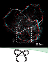
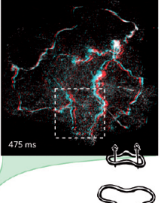
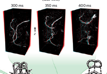
Figure 8: Figures from Kleckner and Irvine (2013) at $t=225$ms, 300ms, 350ms, 400ms and 475ms that correspond roughly to the $t=24$, 36, 42, 45 and 63 figures here. The $t=$300, 350, 400ms frames are side-view close-ups of the region that is outlined in the $t=$225ms and 475ms frames.

Figure 9: Isosurfaces and one vortex line at $t=45$ just after the first reconnection has ended. Vorticity isosurfaces are in blue and the helicity isosurfaces are at $0.1\max(h)$ in green and $0.1\min(h)$ in yellow/orange, where $\max(h)=0.62$ and $\min(h)=-0.26$. A gap without strong vorticity, but twisted and bent vortices to either side, now covers the reconnection zone to the right of red X. Nonetheless, except in that zone, the vortex line seeded at the point of maximum vorticity at X still has the flavour of the original trefoil as it circumnavigates the centre twice and passes through regions with large vorticity and large helicity of both signs. Green $h>0$ positive helicity overlying twisted blue vorticity dominates to the right of the gap. Yellow/orange $h<0$ negative helicity dominates to the left of the gap between the black X and red X, with the strongest enstrophy dissipation (7), between blue isosurfaces of vorticity. There is another region of large negative helicity opposite to the reconnection zone in the upper left whose possible importance is discussed in section 3.4.

Figure 9 at $t=45$=5.6$t_{f}$(Q) shows the trefoil as the reconnection gap spreads between the position of $\epsilon_{\omega-m}\!=\!\max(\epsilon_{\omega})$ (red X) on the left and the blue, twisted vorticity isosurfaces to the right. Unlike earlier times, the green trefoil trajectory goes completely around this gap, similar to how the vortex lines in the $t=400$ms$\approx 5.6t_{f}$(KI) frame in figure 8 avoid the region where reconnection ended at $t=350$ms. The separation between the green $h\!>\!0$ helicity isosurface on the left and the yellow/orange $h$$<$0 helicity isosurface on the right has also increased over the $t=42$ separation in figure 7b.

Furthermore, the extent of all of the $\pm h$ isosurfaces grows, with the positive green helicity to the right of gap more obviously surrounding and covering the twisted blue vorticity isosurfaces where small-scale enstrophy is growing. To the left of the reconnection gap, near the X at $\|\omega\|_{\infty}$, the negative yellow/orange helicity is between, but not on, the sharp bends in the blue vorticity isosurfaces and could be connecting to the $h<0$ yellow/orange helicity isosurfaces in the outer parts of the trefoil, as discussed in section 3.4.

Now that the similarities at and post-reconnection between the simulation graphics at $t=42$ and 45 to the experiments at $t=350$ and 400ms have been identified, one can go back in time to look for similarities between the $t$=300ms experimental image in figure 8 and the trefoil structures in the $t=31$ and 36 figures. In particular, comparing where the loops clearly cross in the $t$=300ms image to the region about the orange X in figure 5 at $t=31$, the location where its loops cross and bend back upon themselves in preparation for reconnection. Further back in time, where the experimental $t$=225ms frame has a kink on the left side of the highlighted box might be similar to the kink underneath the red and yellow + signs in figure 4 at $t=24$ which $h<0$ is flowing out of.

In summary, the steps in forming the reconnection gap are:

• At $t=36$ in figure 6, the gap begins to form where the dissipation of both the vorticity and helicity, of both signs, is greatest.

• After reconnection ends at $t\approx 40$, figure 7 at $t=42$ shows that there are twisted vortex lines on either side of the reconnection gap with only one vestigial piece of the original trefoil vortex that avoids the gap.

• And by $t=45$ in figure 9, the break in the original trefoil is largely complete.

By all these measures, it is the formation of the reconnection gap that marks the end of the first reconnection and justifies using this timescale for comparisons with the experiments. Furthermore, the formation of the reconnection gap marks the beginning of the new phase of even stronger enstrophy growth that leads to the development of the dissipation anomaly starting at $t_{\epsilon}\approx 2t_{x}$ in figure 2a.

3.3 Scheeler et al. (2014) timescales

As noted at the end of section 2.2, using $r_{f}$, C and U from Scheeler et al. (2014b) in (22) gives a nonlinear timescale of $t_{f}$(SK)=168ms, which implies a reconnection time of $t_{x}=860$ms, after the experiment ends. However, using a visual time based upon comparing the frames from its S4 movie at $t=$596ms, 638ms and 658ms, times at which the bubbles marking the vortices disperse then reform, to the physical structures at $t=36$, 41 and 45 here, suggests that the end of the first reconnection should be at $t_{x}$(SK)=638ms. This is consistent with the conclusion of Scheeler et al. (2014b) and is when they changed the colour of one of the subsequent loops in the S4 movie. Based upon $t_{x}\approx 5t_{f}$(SK) for the simulations, this would suggest that for the Scheeler et al. (2014) experiment, the nonlinear timescale should be $t_{f}({\rm SK})=128$ms. Inconsistent with the camber-corrected timescale.

Is there a diagnostic that could be extracted from the available experimental data that could resolve this inconsistency? One measurement would be the initial vertical motion of the entire trefoil structure, whose value for the Q-trefoils agrees with the estimate given by (18). This could be extracted from the experimental trefoil movies. Another possibility is that there is a dynamically viscous timescale at $t_{x}$ that depends upon the thicknesses $r_{e}$ of the filaments. For example $\delta t_{\nu}=T_{c}(\nu)-t_{x}$ using the linearly extrapolated $T_{c}(\nu)$ from figure 2,

Figure 10: Profiles in $y$ of ${\cal H}(y)$ and $E(y)$ (23) and isosurfaces at $t=63$ as reconnection is ending. $E_{m}=\max(E(y))$ and $Z_{m}=\max(Z(y))$ (23). The isosurfaces are for vorticity in blue, with $0.32\|\omega\|_{\infty}$ where $\|\omega\|_{\infty}=3.2$ is at the black X. $h>0$ isosurfaces in green are for $0.05\max(h)$ where $\max(h)=-0.41$. $h<0$ isosurfaces in yellow/orange are for $0.05\min(h)$ where $\min(h)=-0.34$. The advected position where reconnection began is indicted by the red X in a gap between blue $|\omega|$ and green $h>0$ isosurfaces. A blue vortex line that was seeded at $\|\omega\|_{\infty}$ is followed for two circumnavigations of the trefoil before it was terminated at the blue + near $\|\omega\|_{\infty}$. Using (13) with two parallel trajectories, its non-integer self-linking number is ${\cal L}_{S}=-0.26$.

3.4 Late times and negative helicity

The $t\leq t_{x}$ evolution not only generates the first reconnection, it also leads to the next stage during which the global helicity ${\cal H}$ begins to decay slowly and the dissipation $\epsilon=\nu Z$ saturates, possibly generating a finite time, viscosity-independent dissipation anomaly. The following discussion using figures 9 and 10 at $t=45$ and 63 is a first step in determining the physical structures during this period. The emphasis will be on localised negative helicity $h<0$, its growth and role, more than the global ${\cal H}$ and $\epsilon$.

First, a review of $h<0$ creation for $t\leq 45$. Production of $h<0$ was noted as a precursor to reconnection at early times using figure 4 at $t=24$ and then at $t=36$ in figure 6 it was shown that the dissipative production of $h<0$ compensated for the dissipative growth of $h>0$. Isosurfaces of the transport of $h<0$, $\mbox{\boldmath$u$}\cdot\nabla h$ leading out of the reconnection zone were also noted. In section 3.2 it was noted how yellow/orange $h<0$ forms to the left of the reconnection gap and $h>0$ dominates the region to its right in the $t=42$ and 45 figures.

Those observations can be connected to the continuing growth of the enstrophy $Z$ for $t\!>\!t_{x}\!=\!40$ as follows. To the right at $t=45$, the twisted blue isosurfaces of enstrophy that are within a growing green envelope of $h>0$ are reminsicent of the post-reconnection swirling vortices seen for anti-parallel reconnection (Kerr  2013). However, since the global helicity ${\cal H}$ is preserved and therefore could suppress the growth of $h>0$ associated with the enstrophy growth, the formation of the following regions of $h\!<\!0$ relax this constraint. First, to the left of $\|\omega\|_{\infty}$ where the effect of the $h\!<\!0$ dissipation production region shown in figure 6 at $t=36$ would be most immediate, $h<0$ isosurfaces form between bends in the enstrophy surfaces. Due to those bends, $h<0$ is not tied to the local enstrophy $Z$ and therefore cannot accumulate, so transport of $h<0$ out of the vicinity of the reconnection gap is needed.

Second, transport of $h<0$ can be identified by carefully comparing where in figure 6 at $t=36$ there are $\mbox{\boldmath$u$}\cdot\nabla h>0$ isosurfaces for the transport of $h<0$ and where in the $t=42$ and 45 figures there are $h<0$ regions outside the reconnection zone. This includes a small $\mbox{\boldmath$u$}\cdot\nabla h>0$ isosurface at the top of figure 6, which seems too insignificant to account for the large $h<0$ yellow/orange region in the equivalent location at $t=45$ in the upper left of figure 9. The origin of this negative helicity could be the vorticity transport term in (8) a term that originates from the vortex stretching term in (5). In figure 7a at $t=42$, vortex stretching is indicated by how the outer loop at the top has separated from the rest of the trefoil.

Figure 10 at $t=63$ uses $y$-profiles of the helicity, energy and enstrophy, (6, 7, 8)

$${\cal H}(y)=\int hdx\,dz,\quad E(y)=\int edx\,dz,\quad{\rm and}\quad Z(y)=\int|\omega^{2}|dx\,dz$$ (23)

in the upper frame and a top-down three-dimensional perspective in the main frame to show the trefoil as the helicity is beginning to decay and the enstrophy growth is saturating. The upper frame shows that $E(y)$ and ${\cal H}(y)>0$ are concentrated in the centre of the trefoil. There are two regions of ${\cal H}(y)<0$, one off-centre to the right and one to the left at $y\approx 8$.

Note the following two properties of the lower three-dimensional image. Where reconnection began in figure 5 at $t=31$ (red X), there is at $t=63$ a large gap in the enstrophy and $h>0$ isosurfaces whose disappearance could represent the beginning of the decay of the large positive global helicity ${\cal H}$ and saturation of the growth the enstrophy $Z$. The other property is the significant $h<0$ isosurface along the outer loop to the left. This is the continuation of large, outer $h<0$ region noted at $t=42$ and 45, which combined with the $y$-profile at the top clearly shows that this $h<0$ region is outside the original envelope of the trefoil.

This $y>8$, $h<0$ region is tenuously connected to what was the reconnection zone (red X) by the blue vortex line that originates at the new position of $\|\omega\|_{\infty}$ at the bottom the figure, runs through the yellow $y>8$, $h<0$ region then through the vicinity of the red X twice. This supports the evidence from figure 7a that the origin of this negative helicity region could be the vorticity transport term in (8).

Although this single vortex line at $t=63$ retains the basic features of the trefoil, $t=63$ represents one of the last times that the overall trefoil structure can be seen as it breaks apart. Overall, this is similar to the $t=$475ms frame of figure 8. Note that this line terminates at the blue (+) that is near, but not at, $\|\omega\|_{\infty}$ (X), and has many twists. The result is that its self-linking number is ${\cal L}_{S}=-0.26$, a small, non-integer.

4 Conclusion

This paper has presented the structural transformation of a trefoil vortex knot from the first signs of reconnection, past when that reconnection finishes and on to when helicity decay and finite dissipation begins.

Previously, the experiments indicated preservation of the centreline helicity despite a change in the topology. The simulations in Kerr (2017) supported this conclusion by tracking the global helicity ${\cal H}$ (8) as the trefoil loops began to reconnect. In addition, a new enstrophy scaling regime using $B_{\nu}(t)=(\sqrt{\nu}Z(t))^{-1/2}$ (1) was identified over this period with $\nu$-independent crossing of $B_{\nu}(t)$ at a fixed time $t_{x}$. Self-similar $\nu$-independent collapse using (3) was then found for both the Q-trefoils and new anti-parallel reconnection calculations (Kerr  2017). The anti-parallel calculations showed that $t_{x}$ is also when the first reconnection ended and for the Q-trefoil, figures 6, 7 and 9 at $t=36$, 42 and 45 here show that $t_{x}$(Q)=40 is also when the first reconnection of the Q-trefoils ends.

Besides clearly identifying the structure of the trefoil as reconnection ends, the goal here has been to examine the dynamics underlying the evolution of these global properties. Evidence for how viscous reconnection eats through the original trefoil loops is demonstrated using an example of how newly reconnected vorticity can be generated in figure 5 at $t=31$ and by the close-up in figure 7b with vortex lines avoiding a newly created gap in the vorticity isosurfaces. This leads to a clear reconnection gap forming at $t=45$ in figure 9, similar to the gaps that are used to identify equivalent reconnection times in the two experiments considered.

The physical space relationships between the diagnostic terms in the enstrophy and helicity budget equations (7,8) are used to tie together different aspects of this single phenomena and to investigate what role the unexpected preservation of helicity has in generating the new enstrophy scaling regime. From this, it is found that negative helicity plays a role in every step. This starts during the re-alignment of the trefoil loops before physical reconnection begins in figure 4 at $t=24$ and continues with the identification of regions of oppositely signed helicity dissipation in figure 6 at $t=36$ that can explain why the global helicity ${\cal H}$ can be preserved despite a change in the topology.

During this process, $h<0$ is created not only by the dissipative terms, but also by the vorticity transport term and advection in (8). The generation of large-scale negative helicity is demonstrated at $t=45$ and 63 in figures 9 and 10 and appears to be a necessary condition for the enstrophy to continue to grow within the original envelope of the trefoil as simulations with decreasing $\nu$ are run. One can view this as an exhaust mechanism that allows the small-scale vorticity, enstrophy and positive $h>0$ helicity to cascade together to ever smaller scales without being suppressed by the global helicity ${\cal H}$. A dynamical property that would not have been noticed without the experimental results on helicity preservation (Scheeler et al.  2014).

This process continues until the trefoil structure finally begins to break apart at $t=$63 in figure 10, which is roughly when the global helicity ${\cal H}$ begins to decay in figure 3 and the dissipation rate $\epsilon=\nu Z$ saturates in figure 2.

Does this occur in the experiments? To cement the connection with the experiments, a strong correspondence between the evolution of the simulated Q-trefoil and the graphics for the earlier Kleckner and Irvine (2013) experiment in figure 8 has been demonstrated.

Finally, if the $h<0$ exhaust is ever impeded by the periodic boundaries, then we have a physical mechanism for suppressing for enstrophy growth for flows with strong periodicity or symmetries that complements the mathematical bounds proven by Constantin (1986). Fortunately, those bounds can be relaxed simply by increasing the size $\ell$ of the periodic $\ell^{3}$ domains to far beyond the traditional $(2\pi)^{3}$ domain (Kerr  2017) and it seems plausible that unbounded growth of the enstrophy $Z$ is allowed as $\nu\!\to\!0$, which could allow the formation of a dissipation anomaly. That is finite energy dissipation in a finite time as $\nu\to 0$ from smooth solutions, without invoking singularities or roughness.

References

References

- [1]
- [2] [] Biferale L. and Kerr R.M. 1995 Phys. Rev. E 52, 6113–6122.
- [3]
- [4] [] Calugareanu G. 1959 Res. Math. Pures Appl. 4, 5–20.
- [5]
- [6] [] Constantin P. 1986 Commun. Math. Phys. 104, 311–326.
- [7]
- [8] [] Houghton E.L. and Carpenter P.W. 2003 Aerodynamics for Engineering Students, 5th ed.. Butterworth-Heinemann..
- [9]
- [10] [] Kerr R.M. 2005 Fluid Dyn Res 36, 249–260.
- [11]
- [12] [] Kerr R.M. 2013 Phys. Fluids 25, 065101.
- [13]
- [14] [] Kerr R.M. 2017 J. Fluid Mech. submitted, .
- [15]
- [16] Rorai C., Skipper J. Kerr R.M. and Sreenivasan K.R. 2016 J. Fluid Mech. 808, 641–667.
- [17]
- [18] [] Kleckner D. and Irvine W.T.M 2013 Nature Phys. 9, 253–258.
- [19]
- [20] [] Laing C. E., Ricca R.L and Sumners D.W.L. 2015 Sci. Rep. 5, 9224.
- [21]
- [22] [] Moffatt H.K. 1969 J. Fluid Mech. 35, 117–129.
- [23]
- [24] [] Moffatt H.K. 2014 Proc. Nat. Acad. Sci. 111, 3663–3670.
- [25]
- [26] [] Moffatt H.K. and Ricca R. 1992 Proc. Roy. Soc. Math. Phys. Eng. Sci. 439(1906), 411-–429.
- [27]
- [28] [] Sahoo G., Bonaccorso F. and Biferale L. 2015 Phys. Rev. E 92, 051002.
- [29]
- [30] [] Scheeler M. W. Kleckner D. Proment D., Kindlmann G. L. and Irvine W.T.M. 2014 Proc. Nat. Acac. Sci. 111, 15350–15355.
- [31]
- [32] [] Scheeler M. W. Kleckner D. Proment D., Kindlmann G. L. and Irvine W.T.M. Supporting information for Scheeler et al. (2014). www.pnas.org/cgi/content/short/1407232111.
- [33]