Matrix product states for topological phases with parafermions

Abstract

In the Fock representation, we propose a framework to construct the generalized matrix product states (MPS) for topological phases with $\mathbb{Z}_{p}$ parafermions. Unlike the $\mathbb{Z}_{2}$ Majorana fermions, the $\mathbb{Z}_{p}$ parafermions form intrinsically interacting systems. Here we explicitly construct two topologically distinct classes of irreducible $\mathbb{Z}_{3}$ parafermionic MPS wave functions, characterized by one or two parafermionic zero modes at each end of an open chain. Their corresponding parent Hamiltonians are found as the fixed point models of the single $\mathbb{Z}_{3}$ parafermion chain and two-coupled parafermion chains with $\mathbb{Z}_{3}\times\mathbb{Z}_{3}$ symmetry. Our results thus pave the road to investigate all possible topological phases with $\mathbb{Z}_{p}$ parafermions within the matrix product representation in one dimension.

I Introduction

Topological phases of matter have become one of the most important subjects in condensed matter physics, because their low-energy excitations have potential use for fault-tolerant quantum computationRMP . Among them, the simplest class is the symmetry protected topological (SPT) phases with robust gapless edge excitationsChen-Gu-Wen-2011 ; Schuch ; chen-gu-liu-wen ; Chen-Gu-Wen-2011(2) . Without breaking the protecting symmetry or closing the energy gap, these SPT phases can not be continuously connected to the trivial phase. In one dimension, matrix product states (MPS) for bosonic SPT phases capture not only the model dependent microscopic properties of quantum spin chain systems, but also the universal properties associated to the family of Hamiltonians in the same quantum phaseHaldane2008 ; Pollman2010 ; Pollman2012 ; RaoWanZhang2014 ; Fu2014 ; RaoZhangYang2016 . In the valence-bond-solid pictureAKLT , the important feature of these SPT phases is revealed as the edge particles with fractionalized degrees of freedom, resulting in the degeneracy of the entanglement spectrum.

The fractionalized Majorana/parafermion zero modes also exist in fermionic SPT phases and exhibit non-abelian statisticsKitaev2001 ; FidkowshiKitaev ; Fendley2012 , however, it is not straight forward to extend the matrix product representation to the class of fermionic/parafermionic systems. Recently, it is noticed that the fermionic MPS can be constructed by using the language of super vector spacesBultinck2017 ; Kapustin2016 , where the basis states have a well-defined parity of the fermion number. By including additional symmetries, all the topological phases in terms of Majorana fermions have been classified within the matrix product representationBultinck2017 ; Kapustin2016 . If the MPS for topological phases with parafermions are constructed, we have to generalize the concept of fermionic parity and establish the associated basis states.

In this paper, we introduce an intuitive ”particle-like” representation of parafermions in real spaceCobaneraOrtiz , the generalization of Majorana fermions in the Fock space. By a local transformation, these Fock parafermions are connected to the (Weyl) parafermions introduced from the $\mathbb{Z}_{p}$ spin degrees of freedom ($p$ is an integer number). The indistinguishable Fock parafermions satisfy the correlated $p$-exclusion and $2\pi/p$-exchange statisticsCobaneraOrtiz . In the Fock parafermion representation, a natural formulation of the generalized MPS for topological phases with parafermions can be established. For $p=3$, only two topologically distinct classes of irreducible parafermionic MPS can be constructed, characterized by the presence of one or two parafermionic zero modes at each end of open chains. The derived parent Hamiltonians are found as the fixed point lattice models of the single $\mathbb{Z}_{3}$ parafermion chainFendley2012 and two-coupled parafermion chains with $\mathbb{Z}_{3}\times\mathbb{Z}_{3}$ symmetryPollmann2013 . For the topological parafermionic MPS states protected by the $\mathbb{Z}_{3}\times\mathbb{Z}_{3}$ symmetry, there also exists two nontrivial distinct classes, resulting from two different ways to stack the MPS wave functions for two separate $\mathbb{Z}_{3}$ parafermion chains. So our general framework can be easily generalized to construct the $\mathbb{Z}_{p}$ symmetric MPS for one-dimensional topological phases. When additional symmetries are included into the $\mathbb{Z}_{p}$ parafermionic chains, we can classify all the possible topological phases. Moreover, our present formulation can also be used to construct the tensor product states for topological phases in more than one spatial dimensionGu-Verstraete-Wen ; Eisert ; VerstraeteMPO .

In Sec.II, we discuss the Fock space of parafermions and their relations to the Weyl parafermions. Then in Sec. III, we outline the general framework to construct the MPS wave functions in the Fock representation of parafermions. In Sec. IV, we explicitly derive the MPS wave functions for the $\mathbb{Z}_{3}$ parafermion chain and two-coupled $\mathbb{Z}_{3}\times\mathbb{Z}_{3}$ symmetric parafermion chains with various boundary conditions. Conclusion and outlook are given in Sec. V.

II Fock parafermions

It is known that, from the $\mathbb{Z}_{p}$ spin degrees of freedom of the clock models, the parafermions are usually defined by a generalized Jordan-Wigner transformation asFradkinKadonoff ; AlcarazKoberle

$$\chi_{2l-1}=\left(\prod_{k<l}\tau_{k}\right)\sigma_{l},\quad\chi_{2l}=-e^{i\pi/p}\left(\prod_{k\leq l}\tau_{k}\right)\sigma_{l},$$ (1)

where the $\mathbb{Z}_{p}$ spin matrices are given by

$$\tau_{l} = \left(\begin{array}[]{ccccc}0&0&\cdots&0&1\\ 1&0&\cdots&0&0\\ 0&1&\cdots&0&0\\ \vdots&\vdots&\ddots&0&0\\ 0&0&\cdots&1&0\end{array}\right),$$ (7)

$$\sigma_{l} = \text{diag}\left(1,\omega,...,\omega^{p-2},\omega^{p-1}\right),$$ (8)

and $\omega=e^{i2\pi/p}$ ($\bar{\omega}=e^{-i2\pi/p}$). From the relations satisfied by the $\mathbb{Z}_{p}$ spin operators

$$\sigma_{l}^{p}=\tau_{l}^{p}=1,\quad\sigma_{l}\tau_{m}=\omega^{\delta_{l,m}}\tau_{m}\sigma_{l},$$ (9)

the algebra of the parafermions are determined as

$$\chi_{l}^{p}=1,\quad\chi_{l}\chi_{m}=\omega\chi_{m}\chi_{l},\quad\text{for }l<m.$$ (10)

Since the algebra realized by the parafermions is the generalized Clifford algebra first noticed by WeylWeyl1950 , such parafermions are referred to as Weyl parafermions. When $p=2$, they are just Majorana fermions.

It is known that the combinations of two Majorana fermions form one Dirac fermion, and the states of Fock space are endowed with the parity of fermion number, so the creation and annihilation operators can be defined systematically. What is the second quantized description of the Weyl parafermions? It is given by the Fock parafermionsCobaneraOrtiz . With the basis of orthogonal single-particle orbitals: $\phi_{1}$,$\phi_{2}$,$...,\phi_{L}$, the many-body states of $\mathbb{Z}_{p}$ Fock parafermions can be assumed as $|i_{1}i_{2}\cdots i_{L}\rangle$, where $i_{1}$, $i_{2}$, $\cdots$, $i_{L}$ are the respective occupation numbers of the single particle orbitals and $i_{l}\in\mathbb{Z}_{p}\equiv\left\{0,1,2,\cdots,p-1\right\}$. The general structure of the Fock space can be defined by

$$\mathbb{V}_{F}=\bigoplus_{M=0}^{L(p-1)}\text{Span}\left\{|i_{1}i_{2}\cdots i_{L}\rangle,|\sum_{l=1}^{L}i_{l}=M\right\}.$$ (11)

In the following we use the abbreviated notation $|i_{l}\rangle=|0\cdots i_{l}\cdots 0\rangle$ for single-particle states. By considering the non-trivial statistics of Weyl parafermions, the graded tensor product $\otimes_{g}$ should be introduced when constructing the many-body states from the single-particle states,

$$\langle i_{1}i_{2}\cdots i_{L}| = \langle i_{L}|\otimes_{g}\cdots\otimes_{g}\langle i_{2}|\otimes_{g}\langle i_{1}|,$$

$$|i_{1}i_{2}\cdots i_{L}\rangle = |i_{1}\rangle\otimes_{g}|i_{2}\rangle\otimes_{g}\cdots\otimes_{g}|i_{L}\rangle,$$ (12)

which is the exact mathematical description of the graded structure of Hilbert space in a non-commuting system. The crucial ingredient of the graded tensor product is the following isomorphism $\mathcal{F}$:

$$\mathcal{F}(|i_{l}\rangle\otimes_{g}|j_{m}\rangle) \equiv \omega^{ij}|j_{m}\rangle\otimes_{g}|i_{l}\rangle,$$

$$\mathcal{F}(\langle i_{l}|\otimes_{g}|j_{m}\rangle) \equiv \bar{\omega}^{ij}|j_{m}\rangle\otimes_{g}\langle i_{l}|,$$ (13)

for $l<m$. These multiplication rules capture the correlated $2\pi/p$-exchange statistics of Fock parafermions, which is the crucial point for the construction of the MPS wave functions.

Since the orthogonality

$$\langle i_{1}i_{2}\cdots i_{L}|j_{1}j_{2}\cdots j_{L}\rangle=\prod_{l=1}^{L}\delta_{i_{l},j_{l}},$$ (14)

is required, the contraction $\mathcal{C}$ has to be defined via a mapping $\mathbb{V}_{F}^{\ast}\otimes_{g}\mathbb{V}_{F}\rightarrow\mathbb{C}$, which acts as

$$\mathcal{C}\left(\langle i_{l}|\otimes_{g}|j_{l}\rangle\right)=\langle i_{l}|j_{l}\rangle=\delta_{i_{l},j_{l}}.$$ (15)

With the $2\pi/p$-exchange statistics for different orbitals and the orthogonality relation as well as the property of vacuum state, one can derive the $p$-exclusive principle for the same orbital

$$(|i_{l}=1\rangle)^{\otimes_{g}p}\equiv|i_{l}=p\rangle=0.$$ (16)

So the dimension of the Fock space of parafermions is determined as $p^{L}$.

Moreover, the creation operator $C_{l}^{\dagger}$ of Fock parafermions can be introduced by

$$C_{l}^{\dagger}|i_{1}\cdots i_{L}\rangle = |i_{l}=1\rangle\otimes_{g}|i_{1}\cdots i_{L}\rangle$$ (17)

$$= \bar{\omega}^{\sum_{k<l}i_{k}}|i_{1}\cdots i_{l}+1\cdots,i_{L}\rangle,$$

and the adjoint annihilation operator $C_{l}$ by

$$C_{l}|i_{1}\cdots i_{L}\rangle=\omega^{\sum_{k<l}i_{k}}|i_{1}\cdots i_{l}-1\cdots i_{L}\rangle.$$ (18)

The particle number operator is thus derived as

$${N}_{l}=\sum_{r=1}^{p-1}C_{l}^{\dagger r}C_{l}^{r}.$$ (19)

It can be easily proved that the creation and annihilation operators satisfy the following relations

$$C_{l}^{\dagger p} = 0,\quad C_{l}^{\dagger}C_{m}^{\dagger}=\omega C_{m}^{\dagger}C_{l}^{\dagger},$$

$$C_{l}^{p} = 0,\quad C_{l}C_{m}=\omega C_{m}C_{l},$$

$$C_{l}^{\dagger}C_{m} = \bar{\omega}C_{m}C_{l}^{\dagger},\quad C_{l}C_{m}^{\dagger}=\bar{\omega}C_{m}^{\dagger}C_{l},$$ (20)

for different orbitals $l<m$, while for the same orbitals $l=m$, we have $p-1$ relations

$$C_{l}^{\dagger r}C_{l}^{r}+C_{l}^{p-r}C_{l}^{\dagger\left(p-r\right)}=1,\quad r=1,\cdots,p-1.$$ (21)

For $p=2$, the above algebra for the creation and annihilation operators of Fock parafermions will be reduced to the standard fermion algebra.

A natural question arises as what kind of expressions the Weyl parafermions take in the Fock parafermion representation. It was Cobanera and OrtizCobaneraOrtiz who found the following remarkable relations

$$\chi_{2l-1}=C_{l}+C_{l}^{\dagger\left(p-1\right)},\chi_{2l}=C_{l}\omega^{{N}_{l}}+C_{l}^{\dagger\left(p-1\right)},$$ (22)

which generalize the standard relations between the Majorana fermions and Dirac fermions. Formally we can still regard that the combination of two Weyl parafermions forms one Fock parafermion. Their inverse transformations can also be derived, giving rise to the local transformations between the Fock parafermions and Weyl parafermions

$$C_{l}^{\dagger} = \frac{p-1}{p}\chi_{2l-1}^{\dagger}-\frac{1}{p}\sum_{r=1}^{p-1}\overline{\omega}^{r(r+1)/2}\chi_{2l}^{r}\chi_{2l-1}^{\dagger\left(r+1\right)},$$

$$C_{l} = \frac{p-1}{p}\chi_{2l-1}-\frac{1}{p}\sum_{r=1}^{p-1}\omega^{r(r+1)/2}\chi_{2l-1}^{r+1}\chi_{2l}^{\dagger r}.$$ (23)

Interestingly, these transformations are linear for $p=2$ but become nonlinear for $p>2$.

Finally, a charge operator on a lattice site can be defined by $Q_{l}=\chi_{2l-1}^{\dagger}\chi_{2l}=\omega^{N_{l}}$, which yields the relation between charge operator and the particle number operator of the Fock parafermions. The global charge operator is thus given by

$$Q=\prod_{l}Q_{l}=\omega^{\sum_{l}{N}_{l}},$$ (24)

and the global charge in the basis of the Fock space is determined by

$$Q|I\rangle=Q|i_{1}i_{2}\cdots i_{L}\rangle=\omega^{i_{1}+i_{2}+\cdots+i_{L}}|i_{1}i_{2}\cdots i_{L}\rangle.$$ (25)

Then the charge of the many-body basis state $|I\rangle$ denotes as $|I|=\left(\sum_{l=1}^{L}i_{l}\right)$ $\mathrm{mod}$ $p$, while the charge of the basis state $\langle I|$ as $-|I|$. The tensor constructed by the graded tensor product of Fock states with a definite charge has the total charge given by the summation of the charges of these states ($\mathrm{mod}$ $p$). For example, the total charge of the tensor $|I\rangle\otimes_{g}\langle J|$ is given by $\left(|I|-|J|\right)$ $\mathrm{mod}$ $p$. Since the $\mathbb{Z}_{p}$ parafermionic system with $p$ as a prime number always preserves the $\mathbb{Z}_{p}$ symmetryQuella , which is generated by the total charge operator $Q$, we expect that every parafermionic many-body state formed by a linear superposition of the same charge states should have a definite charge.

III MPS in the Fock representation

To construct the MPS for physical degrees of freedom in dimension $d$, we have to introduce two auxiliary virtual degrees of freedom in dimension $D$. Two virtual degrees of freedom on the neighboring sites form a maximally entangled state, and two auxiliary virtual degrees of freedom on the same site are projected onto the physical degrees of freedom. Such a picture captures the most important entanglement property of one-dimensional systems satisfying the area law theorem. With the Fock parafermions, we can write down the local tensor

$$\mathbf{A}[l]=\sum_{\alpha\beta i}A[l]_{\alpha\beta}^{i}|\alpha_{l})\otimes_{g}|i_{l}\rangle\otimes_{g}(\beta_{l+1}|,$$ (26)

where $l$ denotes the site index and $|\alpha_{l})$ and $(\beta_{l+1}|$ stand for the virtual states with the charges $|\alpha|,-|\beta|\in\mathbb{Z}_{p}$ respectively, while $|i_{l}\rangle$ for the physical state with the charge $|i|\in\mathbb{Z}_{p}$ in the Fock space. We can graphically represent $\mathbf{A}[l]$ as shown in Fig.1(a). It is the tensor $\mathbf{A}[l]\in\mathbb{V}_{l}\otimes_{g}\mathbb{H}_{l}\otimes_{g}\mathbb{V}_{l+1}^{\ast}$ that maps from the virtual Hilbert space to the physical Hilbert space. Sometimes we neglect the symbol $\otimes_{g}$ and simply write $\mathbf{A}[l]=\sum_{\alpha,\beta,i}A[l]_{\alpha\beta}^{i}|\alpha_{l})|i_{l}\rangle(\beta_{l+1}|$. One may think that a single Fock parafermion is composed of two Weyl parafermions, so the virtual degrees of freedom should be expressed by Weyl parafermions. Although we still use the Fock representation to express the virtual degrees of freedom, these degrees of freedom of the virtual space are nevertheless fractionalized and describe fractionalized parafermionic zero modes at the ends of open chains. Because the virtual states $|\alpha)$ and $(\beta|$ are not independent, there is a constrain of a fixed charge value $|i|+|\alpha|-|\beta|$ for a local tensor. In other words, since we are unable to use the fractionalized virtual degrees of freedom $\sqrt{p}$ to construct the MPS, we have to employ the unfractionalized degrees of freedom with a constrain of charge to restrict the degrees of freedom. For example, when the fermionic MPS for the single Majorana fermion chain with open boundary conditions are constructed, there are four different choices to fix the virtual degrees of freedom on two edges, but only two-fold ground state degeneracy is producedBultinck2017 .

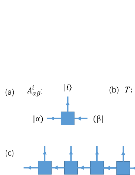
Figure 1: (a) The tensor used to construct MPS, the arrow pointing inward/outward from the box represents the bra/ket state, respectively. (b) Graphical representation of transfer matrix. (c) MPS constructed by contracting the virtual states between the adjacent tensors without fixing the boundaries.

To manipulate the tensor network locally, we will always impose the constraint that all the local tensors $\mathbf{A}[l]$ must have a well-defined charge, so that the different orders of the tensors in the graded tensor product will at most lead to a global phase of the many-body state. To ensure that the tensor $\mathbf{A}[l]$ has a definite charge, we must use the matrices $\mathbf{A}[l]^{i}$ with a well-defined charge. We mainly focus on the translational invariant systems with the same $\mathbf{A}[l]$ on different sites and the site index will be omitted in the following. Then we impose that the charge of the local tensor $\mathbf{A}$ is zero so that the order of the individual tensors $\mathbf{A}$ does not affect the definition of tensor network and its charge is independent on the lattice size. When we contract the virtual bonds by the mapping $\mathcal{C}$, we have the general parafermionic MPS as

$$|\psi\rangle = \mathcal{C}(\mathbf{A}[1]\otimes_{g}\mathbf{A}[2]\otimes_{g}\cdots\otimes_{g}\mathbf{A}[L])$$

$$= \sum_{i_{1}..i_{N}}\sum_{\alpha\beta}\left(A^{i_{1}}\cdots A^{i_{L}}\right)_{\alpha\beta}|\alpha_{1})|i_{1}\cdots i_{L}\rangle(\beta_{L+1}|,$$

which has been shown in Fig. 1(c). Because the charges of $|\alpha_{l})$ and $(\alpha_{l}|$ add up to zero, the contraction does not affect the charge of the state $|\psi\rangle$. Finally, we can choose different boundary conditions to fix the virtual states at the boundaries. Because the commutation relation of parafermions requires a definite order, the translation invariance on a closed chain is not well-defined.

For any MPS wave function, one can construct a local parent Hamiltonian whose ground state is uniquely given by the MPS. The general way to construct the parent Hamiltonian is as follows. First we should block the consecutive $m$ sites so that the rank of the map $B_{\alpha\beta}^{i}=(A^{i_{1}}A^{i_{2}}\cdots A^{i_{m}})_{\alpha\beta}$ with row indices $i$ and the column indices $\alpha\beta$ is smaller than $d^{m}$. Then a local Hamiltonian is obtained by projecting onto the space orthogonal to the image of this map. In physics, the image of this map is the ground state subspace. Since the operator $P=BB^{+}$ is the orthogonal projector onto the image of $B$, where $B^{+}$ is the Moore-Penrose pseudo-inverse of the matrix $B$, we can construct a gapped frustration free parent Hamiltonian by adding all local projectors

$$H=\sum_{l}(1-P_{l}),$$ (28)

where $1-P_{l}$ is the orthogonal projector onto the Hilbert space orthogonal to the image of $B$, the kernel of $B^{+}$. Then, if the local Hamiltonian matrix is simple, i.e., it only involves a few number of lattice sites, we can try to expand it with possible charge zero operators in terms of the parafermion modes defined on those lattice sites. Neglecting the unnecessary terms, the simplified parent Hamiltonian corresponding to the constructed MPS wave function is thus obtained.

IV $\mathbb{Z}_{3}$ parafermionic MPS

Following the general procedures of constructing MPS with $\mathbb{Z}_{3}$ Fock parafermions, the charges of elements of the local matrices $\mathbf{A}^{i}=\sum_{\alpha\beta}A_{\alpha\beta}^{i}|\alpha_{l})\otimes_{g}(\beta_{l+1}|$ (the components of the local tensor) are determined by $(\beta-\alpha)$ $\mathrm{mod}$ $3$, shown in Tab.1. To ensure that the local matrix $\mathbf{A}^{i}$ has a definite charge, we require that the matrix form of $A_{\alpha\beta}^{i}$ must have the following nine blocks structure:

$$A^{i} = \left(\begin{array}[]{ccc}a_{0}&0&0\\ 0&b_{0}&0\\ 0&0&c_{0}\end{array}\right),\quad\text{if\ }|i|=0\text{,}$$ (32)

$$\text{ }A^{i} = \left(\begin{array}[]{ccc}0&a_{1}&0\\ 0&0&b_{1}\\ c_{1}&0&0\end{array}\right),\quad\text{if\ }|i|=1\text{,}$$ (36)

$$\text{\ }A^{i} = \left(\begin{array}[]{ccc}0&0&a_{2}\\ b_{2}&0&0\\ 0&c_{2}&0\end{array}\right),\quad\text{if\ }|i|=2\text{,}$$ (40)

which is determined by the graded structure of Fock space.

	0	2	1
0	0	2	1
1	1	0	2
2	2	1	0

Table 1: The charges of different elements of $\mathbf{A}^{i}$, which reveal the graded structure of $A^{i}$.

Actually these matrices form a family of $\mathbb{Z}_{3}$ symmetric states, and all $A^{i}$ span a $\mathbb{Z}_{3}$ graded algebra. If we multiply some of these matrices $A^{i},A^{j},\cdots,A^{k}$ together to get a blocked matrix $B^{m}=A^{i}A^{j}\cdots A^{k}$ with $|m|=\left(|i|+|j|+\cdots+|k|\right)$ $\mathrm{mod}$ $3$, the blocked matrix $B^{m}$ still satisfies the above conditions. The $\mathbb{Z}_{3}$ graded algebra is the consequence that the system must be $\mathbb{Z}_{3}$ symmetric, so the $\mathbb{Z}_{3}$ charge conserves and the states in the Hilbert space must have a well-defined charge. Hence the MPS with different charges cannot be connected smoothly. Since the $\mathbb{Z}_{3}$ parafermionic system is intrinsically $\mathbb{Z}_{3}$ symmetric, the Hilbert space is naturally a $\mathbb{Z}_{3}$ graded vector space, which is a generalization of super vector space for the $\mathbb{Z}_{2}$ caseBultinck2017 ; Kapustin2016 .

IV.1 Wave functions and parent Hamiltonian

A prototype parafermionic MPS can be defined by the simplest matrices

$$A^{0}=\left(\begin{array}[]{ccc}1&0&0\\ 0&1&0\\ 0&0&1\end{array}\right),A^{1}=\left(\begin{array}[]{ccc}0&1&0\\ 0&0&1\\ 1&0&0\end{array}\right),A^{2}=\left(\begin{array}[]{ccc}0&0&1\\ 1&0&0\\ 0&1&0\end{array}\right).$$

The MPS with open boundary conditions constructed by these matrices can be expressed as

$$|\psi_{n}\rangle=\sum_{\{i_{l}\}}(A^{i_{1}}A^{i_{2}}\cdots A^{i_{L}})_{\alpha\beta}|i_{1}i_{2}\cdots i_{L}\rangle,$$ (41)

where $n=\left(\alpha-\beta\right)$ $\mathrm{mod}$ $3$. Although we have nine different choices of ($\alpha,\beta$) corresponding to nine different boundary conditions, there are only three topologically distinct ground states carrying three $\mathbb{Z}_{3}$ charges $n=0,1,2$, because the $\mathbb{Z}_{3}$ graded structure of the matrices of $A^{i}$ shown in the Tab. 1. Specifically, they are equal wight superpositions of all basis states with the same charge

$$|\psi_{n}\rangle=\sum_{\left(\Sigma_{l}i_{l}\right)\text{ }\mathrm{mod}\text{ }3\text{ }=n}|i_{1}i_{2}\cdots i_{L}\rangle,\text{ }n=0,1,2.$$ (42)

Here we would like to emphasize that the summation has to satisfy the global constrain. Similar MPS state is also considered in the recent paperMazza .

With the parafermionic MPS wave functions, the transfer matrix $T=\sum_{i}A^{i}\otimes\bar{A}^{i}$ which is shown graphically in Fig. 1(b) can be defined, and we can calculate its eigenvalue spectrum. We surprisingly found that there is a unique eigenvalue with three-fold degeneracy, indicating the distinct property of the parafermionic MPS. In the bosonic MPS, however, the degeneracy of the largest eigenvalue of the transfer matrix stems from the spontaneous symmetry breaking in the ground state. But the $\mathbb{Z}_{3}$ symmetry can not be spontaneously broken in the parafermion chain. This result becomes the most striking difference between the bosonic and parafermionic MPS. In this sense, the above matrices $A^{0},A^{1}$ and $A^{2}$ just form a “non-trivial” type of the $\mathbb{Z}_{3}$ graded algebra, which has a non-trivial center formed by these three matrices.

Using the method of deriving the parent Hamiltonian, we can obtain the model Hamiltonian, corresponding to the fixed-point Hamiltonian for the non-trivial phase of a single parafermion chainFendley2012

$$H = -\sum_{l=1}^{L-1}\left[\bar{\omega}^{{N}_{l}-1}\left(C_{l}^{\dagger}C_{l+1}+C_{l}^{\dagger}C_{l+1}^{\dagger 2}\right)\right.$$ (43)

$$\text{ \ \ \ }\left.+\omega\left(C_{l}^{2}C_{l+1}+C_{l}^{2}C_{l+1}^{\dagger 2}\right)+\text{h.c.}\right]$$

$$= -\sum_{l=1}^{L-1}\left(\omega\chi_{2l}^{\dagger}\chi_{2l+1}+\bar{\omega}\chi_{2l+1}^{\dagger}\chi_{2l}\right),$$

where we have used the relations between the Fock parafermions and Weyl parafermions

$$C_{l} = \frac{2}{3}\chi_{2l-1}-\frac{1}{3}\left(\chi_{2l}+\omega\chi_{2l-1}^{\dagger}\chi_{2l}^{\dagger}\right),$$

$$C_{l}^{\dagger} = \frac{2}{3}\chi_{2l-1}^{\dagger}-\frac{1}{3}\left(\chi_{2l}^{\dagger}+\bar{\omega}\chi_{2l}\chi_{2l-1}\right).$$ (44)

In the Fock representation, we notice that the parent Hamiltonian includes the nearest neighbor single-particle and two-particle hopping terms as well as the three-parafermion “pairing” terms on the nearest neighbor sites. However, in terms of Weyl parafermions, the parent Hamiltonian just takes a simple form, the nearest neighbor hopping terms, and we can easily find that the Weyl parafermions $\chi_{1}^{\dagger}$ and $\chi_{2L}$ characterize two edge parafermion zero modes on each end of the open chain. These edge parafermions are fractionalized from the physical degrees of freedom on the lattice sites. Since we can not distinguish three ground states $|\psi_{0}\rangle,|\psi_{1}\rangle,|\psi_{2}\rangle$ locally in the bulk, they are topologically non-trivial degenerate states. In addiction, via the generalized inverse Jordan-Wigner transformation, one can transform the above parent Hamiltonian $H$ into the ferromagnetic $\mathbb{Z}_{3}$ clock model, whose ground state has a long-range order with three-fold degeneracy due to the spontaneous $\mathbb{Z}_{3}$ symmetry breaking.

Since the coupling parameters can be rotated by an angle $\pm 2\pi/3$, we further noticed that there are two other equivalent parent HamiltoniansH H Tu

$$H^{\prime} = -\sum_{l=1}^{L-1}\left(\chi_{2l}^{\dagger}\chi_{2l+1}+\chi_{2l+1}^{\dagger}\chi_{2l}\right),$$

$$H^{\prime\prime} = -\sum_{l=1}^{L-1}\left(\bar{\omega}\chi_{2l}^{\dagger}\chi_{2l+1}+\omega\chi_{2l+1}^{\dagger}\chi_{2l}\right),$$ (45)

whose charges of their corresponding MPS depend on the lattice size. This can be seen from the total charge operator

$$Q = \chi_{1}^{\dagger}\chi_{2}\chi_{3}^{\dagger}\chi_{4}\cdots\chi_{2L-1}^{\dagger}\chi_{2L}$$

$$= \chi_{1}^{\dagger}\left(\bar{\omega}\chi_{3}^{\dagger}\chi_{2}\right)\left(\bar{\omega}\chi_{5}^{\dagger}\chi_{4}\right)\cdots\left(\bar{\omega}\chi_{2L-1}^{\dagger}\chi_{2L-2}\right)\chi_{2L},$$

where the parafermionic operators on the adjacent sites define the “bond charge” $\bar{\omega}\chi_{2l+1}^{\dagger}\chi_{2l}$. Three degenerate ground states with zero bond charge can minimize the energy of the parent Hamiltonian $H$, while the ground states with “bond charge” $2$ and $1$ can make the energies of $H^{\prime}$ and $H^{\prime\prime}$ minimize, respectively. Those MPS wave functions must be approximated by the local tensors $\mathbf{A}$ with charge $2$ and $1$, respectively.

Next we consider the corresponding parafermionic MPS in the closed boundary conditions. A closure tensor $\mathbf{Y}_{a}$ with the charge $a=0,1,2$ can be introduced in the wave function as follows

$$|\psi_{a}\rangle = \mathcal{C}(\mathbf{Y}_{a}\mathbf{\otimes}_{g}\mathbf{A}[1]\otimes_{g}\mathbf{A}[2]\otimes_{g}\cdots\otimes_{g}\mathbf{A}[L])$$ (46)

$$= \sum_{\{i_{l}\}}\text{tr}(Y_{a}^{T}A^{i_{1}}A^{i_{2}}\cdots A^{i_{L}})|i_{1}i_{2}\cdots i_{L}\rangle,$$

where $\mathbf{Y}_{a}\mathbf{=}\sum_{\gamma\delta}Y_{a,\gamma\delta}(\gamma_{1}|\otimes_{g}|\delta_{L})$. The closure tensor $Y$ and the closed wave function are shown in Fig. 2. Since all local tensors $\mathbf{A}$ have charge $0$, the moving of $|\delta_{L})$ to the right end does not bring any phase. Different choices of $\mathbf{Y}_{a}$ just result in the different charges of the closed wave functions in the view of the “boundary charge” as shown

$$Q=\chi_{1}^{\dagger}\chi_{2}\chi_{3}^{\dagger}\chi_{4}\cdots\chi_{2L-1}^{\dagger}\chi_{2L}=\bar{\omega}\left(\chi_{2L}\chi_{1}^{\dagger}\right).$$ (47)

Therefore, we can write the parent Hamiltonians corresponding to the MPS with the closed boundary conditions

$$H^{(a)}=H-\left(\omega^{a}\chi_{2L}^{\dagger}\chi_{1}+\bar{\omega}^{a}\chi_{1}^{\dagger}\chi_{2L}\right),\text{ }a=0,1,2.$$ (48)

Actually the translational invariance of a closed parafermion chain is very tricky. It seems that $H^{(1)}$ is translational invariant, but from the ”bond charge” point of view, it corresponds to the MPS with a charge $2$. By applying the translation operator to the MPS wave functions, we find that none of them satisfies the periodic boundary conditionBultinck2017 . We attribute this to the ordering requirement in the commutation relation of parafermions. From topological bulk response, however, we know that three different boundary conditions can select three different ground states under the open boundary conditions. So we immediately identify

$$Y_{0}=\left(\begin{array}[]{ccc}1&0&0\\ 0&1&0\\ 0&0&1\end{array}\right),Y_{1}=\left(\begin{array}[]{ccc}0&1&0\\ 0&0&1\\ 1&0&0\end{array}\right),Y_{2}=\left(\begin{array}[]{ccc}0&0&1\\ 1&0&0\\ 0&1&0\end{array}\right).$$

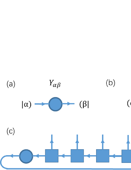
Figure 2: (a) The closure tensor $\mathbf{Y}$. (b) The transpose closure tensor $\mathbf{Y}^{T}$. (c) Parafermionic MPS with closed boundary condition.

IV.2 Stacking two $\mathbb{Z}_{3}$ parafermionic MPS

According to the classification of the $\mathbb{Z}_{p}$ symmetric parafermion chains with a prime integer $p$, there only exist two topologically distinct gapped phasesPollmann2013 ; Quella , including a topological nontrivial phase and trivial gapped phase. We have just constructed one topologically nontrivial $\mathbb{Z}_{3}$ symmetric MPS, and another $\mathbb{Z}_{3}$ ”trivial” type algebra of the parafermionic MPS wave function has not been considered. Similar to the $\mathbb{Z}_{2}$ caseBultinck2017 ; Kapustin2016 , stacking two separate parafermionic MPS in one unit cell will automatically gives rise to the other type parafermionic MPS. We start from the graded tensor product of two different local tensors and record the induced phases. For the local tensors $\mathbf{A}$ with charge $0$, we have

$$\mathcal{F}(\mathbf{A}\otimes_{g}\mathbf{A}^{\prime})$$ (49)

$$= \mathcal{F}\left[\sum_{i\alpha\beta}\left(A_{\alpha\beta}^{i}|\alpha)|i\rangle(\beta|\right)\otimes_{g}\sum_{j\gamma\delta}\left(A_{\gamma\delta}^{\prime j}|\gamma)|j\rangle(\delta|\right)\right]\text{\ \ }$$

$$= \sum_{ij\alpha\beta\gamma\delta}A_{\alpha\beta}^{i}A_{\gamma\delta}^{\prime j}\omega^{|\gamma||i||}|\alpha)|\gamma)|i\rangle|j\rangle(\delta|(\beta|.$$

Then new local matrices building up the stacking MPS are defined by

$$B_{(\alpha\gamma)(\beta\delta)}^{ij}=A_{\alpha\beta}^{i}A_{\gamma\delta}^{\prime j}\omega^{|\gamma||i|}.$$ (50)

With the matrices for the single parafermion chain, we have nine local matrices with the smaller indices arranged before the larger indices. The resulting MPS wave function is

$$|\phi\rangle=\sum_{\{i_{l},j_{l}\}}\left(B^{i_{1}j_{1}}B^{i_{2}j_{2}}\cdots B^{i_{L}j_{L}}\right)_{\alpha\beta}|i_{1}j_{1}i_{2}j_{2}\cdots i_{L}j_{L}\rangle.$$ (51)

If we write down these composite MPS wave functions explicitly, there are $81$ different boundary conditions ($\alpha,\beta$). But only nine topologically different states exist. We also find the entanglement spectrum with a nine-fold degeneracy. Actually when the wave functions are explicitly written down, one can find that the total charges of the even and odd sublattices generated by the operators $Q_{1}=\omega^{\sum_{i}N_{2i-1}}$ and $Q_{2}=\omega^{\sum_{i}N_{2i}}$ are conserved separately. So the stacking MPS wave functions display a larger $\mathbb{Z}_{3}\times$ $\mathbb{Z}_{3}$ symmetry.

Furthermore, according to the bosonic and fermionic MPSBultinck2017 , it is expected that the parafermionic MPS is reducible when the local matrices do not span a simple $\mathbb{Z}_{3}$ graded algebra. Via the following gauge transformation

$$G=\frac{\sqrt{3}}{3}\left(\begin{array}[]{ccccccccc}\omega&0&0&\bar{\omega}&0&0&1&0&0\\ 1&0&0&\bar{\omega}&0&0&\omega&0&0\\ 1&0&0&1&0&0&1&0&0\\ 0&0&\omega&0&0&\bar{\omega}&0&0&1\\ 0&0&1&0&0&\bar{\omega}&0&0&\omega\\ 0&0&1&0&0&1&0&0&1\\ 0&\omega&0&0&\bar{\omega}&0&0&1&0\\ 0&1&0&0&\bar{\omega}&0&0&\omega&0\\ 0&1&0&0&1&0&0&1&0\end{array}\right),$$ (52)

those local matrices can be transformed into nine block diagonal matrices, and the phase difference in diagonal blocks just causes a global phase change. Hence $B^{ij}$ can be reduced to nine $3\times 3$ matrices

$$B^{00} = \left(\begin{array}[]{ccc}1&0&0\\ 0&1&0\\ 0&0&1\end{array}\right),B^{10}=\left(\begin{array}[]{ccc}0&0&\bar{\omega}\\ \omega&0&0\\ 0&1&0\end{array}\right),$$ (59)

$$B^{01} = \left(\begin{array}[]{ccc}0&0&1\\ 1&0&0\\ 0&1&0\end{array}\right),B^{11}=\left(\begin{array}[]{ccc}0&\bar{\omega}&0\\ 0&0&\omega\\ 1&0&0\end{array}\right),$$ (66)

$$B^{02} = \left(\begin{array}[]{ccc}0&1&0\\ 0&0&1\\ 1&0&0\end{array}\right),B^{12}=\left(\begin{array}[]{ccc}\bar{\omega}&0&0\\ 0&\omega&0\\ 0&0&1\end{array}\right),$$ (73)

$$B^{20} = \left(\begin{array}[]{ccc}0&\bar{\omega}&0\\ 0&0&1\\ \omega&0&0\end{array}\right),B^{21}=\left(\begin{array}[]{ccc}\bar{\omega}&0&0\\ 0&1&0\\ 0&0&\omega\end{array}\right),$$ (80)

$$B^{22} = \left(\begin{array}[]{ccc}0&0&\bar{\omega}\\ 1&0&0\\ 0&\omega&0\end{array}\right).$$ (84)

These matrices form the “trivial” type of $\mathbb{Z}_{3}$ graded algebra, which is nothing but ungraded algebra, because its center is an identity. For the closed boundary condition, there is a unique ground state so that the two sublattice symmetries cannot be broken. The final wave functions are also the superpositions of states with the same sublattice charges.

By combining two closure matrices, we can find the closure matrix for the stacking MPS. For example, two charge $1$ closures give rise to

$$\mathbf{Y} = \mathbf{Y}_{1}\otimes_{g}\mathbf{Y}_{2}$$ (85)

$$\mathbf{=} \sum_{\alpha\beta}Y_{1,\alpha\beta}(\alpha_{1}|\otimes_{g}|\beta_{1})\sum_{\gamma\delta}Y_{2,\gamma\delta}(\gamma_{2}|\otimes_{g}|\delta_{2})$$

$$= \sum_{\alpha\beta\gamma\delta}Y_{(\alpha\gamma)(\beta\delta)}(\gamma_{2}|(\alpha_{1}|\otimes_{g}|\beta_{1})|\delta_{2}),$$

where $Y_{(\alpha\gamma)(\beta\delta)}=Y_{1,\alpha\beta}Y_{2,\gamma\delta}\omega^{|\gamma|}$. After the gauge transformation, $Y^{T}$ can be reduced to

$$Y^{T}=\left(\begin{array}[]{ccc}0&0&1\\ \omega&0&0\\ 0&\bar{\omega}&0\end{array}\right),$$

and the corresponding MPS wave function is thus given by

$$|\phi\rangle=\sum_{\{i_{l},j_{l}\}}\text{tr}(Y^{T}B^{i_{1}j_{1}}B^{i_{2}j_{2}}\cdots B^{i_{L}j_{L}})|i_{1}j_{1}i_{2}j_{2}\cdots i_{L}j_{L}\rangle.$$

This is the total charge-$2$ MPS with total sublattice charge ones on each sublattice. It should be pointed out that the ground state properties in the reducing procedure do not change under the closed boundary conditions only. In the open boundary conditions, however, the gauge transformation induces a linear combination between the degenerate ground states, and then the reduced MPS breaks the $\mathbb{Z}_{3}\times\mathbb{Z}_{3}$ symmetry.

Furthermore, we can also calculate the eigenvalues of the transfer matrix $T^{\prime}=\sum_{ij}B^{ij}\otimes\bar{B}^{ij}$, but its unique eigenvalue is nondegenerate. The non-degenerate of the eigenvalue just suggests the “trivial” type of $\mathbb{Z}_{3}$ graded algebra of $B^{ij}$, similar to the bosonic MPS for one-dimensional topological phases. Thus, from the $\mathbb{Z}_{3}\times\mathbb{Z}_{3}$ symmetry point of view, the stacking MPS wave function should belong to the family of SPT phases. This manifests from the following analysis. Requiring

$$V_{1}B^{ij}V_{1}^{-1} = \sum_{i^{\prime}j^{\prime}}U_{ij,i^{\prime}j^{\prime}}^{(1)}B^{i^{\prime}j^{\prime}},\text{ }$$

$$V_{2}B^{ij}V_{2}^{-1} = \sum_{i^{\prime}j^{\prime}}U_{ij,i^{\prime}j^{\prime}}^{(2)}B^{i^{\prime}j^{\prime}}$$ (86)

with $U^{(1)}=\sigma\otimes\mathbb{I}$ and $U^{(2)}=\mathbb{I}\otimes\sigma$ as local unitary transformations on one unit cell and linear representations of $\mathbb{Z}_{3}\times\mathbb{Z}_{3}$ generators, we can find the projective representations of $Q_{1}$ and $Q_{2}$ as

$$V_{1}=\left(\begin{array}[]{ccc}0&0&1\\ 1&0&0\\ 0&1&0\end{array}\right),V_{2}=\left(\begin{array}[]{ccc}0&\bar{\omega}&0\\ 0&0&1\\ \omega&0&0\end{array}\right),$$ (87)

from which we find the important relation

$$V_{1}V_{2}=\bar{\omega}V_{2}V_{1},$$ (88)

with $\bar{\omega}$ as the factor of the projective representation characterizing this SPT phaseChen-Gu-Wen-2011 ; Chen-Gu-Wen-2011(2) ; Geraedts .

Following the procedures to construct the parent Hamiltonian, we can derive

$$H_{2}=-\sum_{l=1}^{L-1}\left[\omega\left(\chi_{4l}^{\dagger}\chi_{4l+3}+\chi_{4l-2}\chi_{4l-1}\chi_{4l}^{\dagger}\chi_{4l+1}^{\dagger}\right)+\text{h.c.}\right],$$ (89)

which commutes with $Q_{1}$ and $Q_{2}$. Note that the same parent Hamiltonian is also obtained by using original matrices. Actually, $H_{2}$ can be viewed from the combination of two independent parafermion chainsPollmann2013 , as shown in the Fig. 3(a). Unlike the $\mathbb{Z}_{2}$ Majorana fermion case, where the system after stacking is two decoupled Kitaev chains and the edge modes are two single edge Majorana operators, the parent Hamiltonian $H_{2}$ describes a two-coupled parafermion chains satisfying the unusual commutation relation of Weyl parafermions. By fractionalizing charge operators on two sublattices separatelyGeraedts , we can find that two parafermion zero modes exist on each end of the two-coupled chains, given by the Weyl parafermions ($\chi_{1}^{\dagger},\chi_{3},\chi_{4L-2}\chi_{4L-1}\chi_{4L}^{\dagger},\chi_{4L}^{\dagger}$) for the chains with $2L$ sites and ($\chi_{1}^{\dagger},\chi_{3},\chi_{4L}^{\dagger},\chi_{4L+2}$) for the chains with $2L+1$ sites. These edge Weyl parafermions commute with parent Hamiltonian and carry $\mathbb{Z}_{3}$ charges. Two zero parafermion modes on the same edge can actually form a physical degree of freedom three. In the case of $2L$ sites, due to the two edges are not symmetric, one of the edge mode is not a single parafermion operator. The complicated edge modes and quartic interactions in the parent Hamiltonian manifest the unusual commutation relation of parafermions, which also endows the parafermion chain the intrinsically strong-coupled propertyH H Tu . The integer edge degrees of freedom actually imply that there is no real fractionalization. Two edge zero modes thus yield total nine-fold degenerate ground states for the open chains. If we introduced the hoping term $\left(\chi_{1}^{\dagger}\chi_{3}+\text{h.c.}\right)$ into the parent Hamiltonian, it would break the $\mathbb{Z}_{3}\times\mathbb{Z}_{3}$ symmetry and gap out the edge modes, so we can thus prove that the edge modes are protected by $\mathbb{Z}_{3}\times\mathbb{Z}_{3}$ symmetry. Actually there is a global unitary transformationSantos

$$W=\exp\left[\frac{i2\pi}{3}\sum_{l}\sum_{a=1}^{p-1}\frac{(\bar{\omega}\chi_{4l-2}^{{\dagger}}\chi_{4l-1})^{a}-(\bar{\omega}\chi_{4l}^{{\dagger}}\chi_{4l+1})^{a}}{(\omega^{a}-1)(\bar{\omega}^{a}-1)}\right],$$ (90)

which can transform the ground state of $H_{2}$ into a trivial gapped phase. But such a unitary transformation explicitly breaks the $\mathbb{Z}_{3}\times\mathbb{Z}_{3}$ symmetry. Therefore, we conclude that the ground state of $H_{2}$ is a SPT phase protected by the $\mathbb{Z}_{3}\times\mathbb{Z}_{3}$ symmetry.

Moreover, in terms of $\mathbb{Z}_{3}$ spin operators via the inverse generalized Jordan-Wigner transformation, this parent Hamiltonian can be expressed as the $\mathbb{Z}_{3}\times\mathbb{Z}_{3}$ cluster modelSantos ; Geraedts

$$H_{2,\text{cl}}=-\sum_{l=1}^{L-1}\left(\sigma_{2l-1}\tau_{2l}\sigma_{2l+1}^{\dagger}+\bar{\omega}\sigma_{2l}^{{\dagger}}\tau_{2l+1}\sigma_{2l+2}+\text{h.c}.\right).$$ (91)

By redefinition of $\tau_{2l-1}$, we can wipe out $\bar{\omega}$ in front of the second term. The ground state of $H_{2,\text{cl}}$ belongs to a SPT phase protected by the $\mathbb{Z}_{3}\times\mathbb{Z}_{3}$ symmetry, which can be proved from the view point of the bosonic matrix product representation.

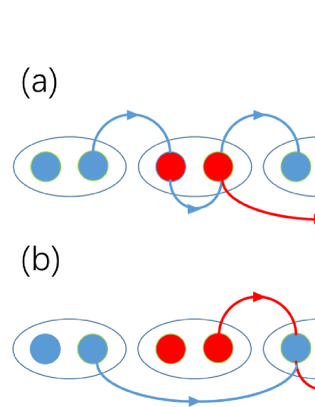
Figure 3: Graphical illustration of parent Hamiltonians $H_{2}$ (a) and $H_{2}^{\prime}$ (b). The ellipses denote different sites, blue and red dots represent Weyl parafermions from original chain-1 and chain-2, respectively. Blue and red lines denote the hopping terms originated from the hopping terms of the chain-1 and chain-2, some of them keep quadratic but others change into quartic form after combination.

IV.3 Another way of stacking

Since the stacking MPS wave function displays the $\mathbb{Z}_{3}\times\mathbb{Z}_{3}$ symmetry in bulk, there should exist another topologically nontrivial gapped phases from the classification theorychen-gu-liu-wen ; Santos . In fact we can obtain another non-trivial SPT phase by stacking of two single parafermion chains in a different recording order:

$$\mathcal{F}\left[\sum_{i\alpha\beta}\left(A_{\alpha\beta}^{i}|\alpha)|i\rangle(\beta|\right)\otimes_{g}\sum_{j\gamma\delta}\left(A_{\gamma\delta}^{\prime j}|\gamma)|j\rangle(\delta|\right)\right]$$ (92)

$$= \sum_{ij\alpha\beta\gamma\delta}A_{\alpha\beta}^{i}A_{\gamma\delta}^{\prime j}\omega^{|j||\beta|}|\gamma)|\alpha)|i\rangle|j\rangle(\beta|(\delta|,$$

where we have assumed that the parafermion site-sequence number of the local tensors $\mathbf{A}$ is larger than that of the local tensors $\mathbf{A}^{\prime}$. Two different recording ways are illustrated in the Fig. 4.

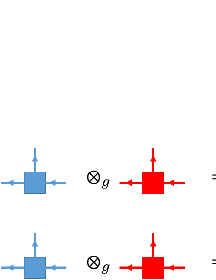
Figure 4: The blue/red graph represents the local tensor in the MPS of the chain-1 or chain-2, and the differences are the recording order of the virtual indices. In the second way of stacking, the index of the chain-1 is larger than that of the chain-2 in the same unit cell.

From the matrices given for the single parafermion chain, we have nine $9\times 9$ local matrices

$$D_{(\gamma\alpha)(\delta\beta)}^{ij}=A_{\alpha\beta}^{i}A_{\gamma\delta}^{\prime j}\omega^{|j||\beta|},$$ (93)

which can also be transformed into block diagonal matrix form by the gauge transformation $G$. We then reduce these local matrices to

$$D^{00} = \left(\begin{array}[]{ccc}1&0&0\\ 0&1&0\\ 0&0&1\end{array}\right),D^{01}=\left(\begin{array}[]{ccc}0&0&\bar{\omega}\\ \omega&0&0\\ 0&1&0\end{array}\right),$$ (100)

$$D^{02} = \left(\begin{array}[]{ccc}0&\bar{\omega}&0\\ 0&0&1\\ \omega&0&0\end{array}\right),D^{10}=\left(\begin{array}[]{ccc}0&0&1\\ 1&0&0\\ 0&1&0\end{array}\right),$$ (107)

$$D^{11} = \left(\begin{array}[]{ccc}0&1&0\\ 0&0&\bar{\omega}\\ \omega&0&0\end{array}\right),D^{12}=\left(\begin{array}[]{ccc}\omega&0&0\\ 0&\bar{\omega}&0\\ 0&0&1\end{array}\right),$$ (114)

$$D^{20} = \left(\begin{array}[]{ccc}0&1&0\\ 0&0&1\\ 1&0&0\end{array}\right),D^{21}=\left(\begin{array}[]{ccc}\omega&0&0\\ 0&1&0\\ 0&0&\bar{\omega}\end{array}\right),$$ (121)

$$D^{22} = \left(\begin{array}[]{ccc}0&0&1\\ \omega&0&0\\ 0&\bar{\omega}&0\end{array}\right),$$ (125)

which also form the “trivial” type $\mathbb{Z}_{3}$-graded algebra. As we pointed out, the $\mathbb{Z}_{3}\times\mathbb{Z}_{3}$ symmetry is preserved for the MPS under the closed boundary condition in the reducing procedure. For a closed boundary condition, the corresponding MPS wave function can be expressed as

$$|\phi^{\prime}\rangle=\sum_{\{i,j\}}\text{tr}(Y^{T}D^{i_{1}j_{1}}D^{i_{2}j_{2}}\cdots D^{i_{L}j_{L}})|i_{1}j_{1}i_{2}j_{2}\cdots i_{L}j_{L}\rangle,$$

with the closure matrix $Y$ which can be derived as well. We notice that the transfer matrix of $|\phi^{\prime}\rangle$ is as same as that of $|\phi\rangle$. One may think that they belong to the same phase, but in our parafermionic case, they differ from each other in several aspects. For the open boundary conditions, if we choose the simple boundary conditions such as $(\alpha,\beta)=(1,1)$, the $\mathbb{Z}_{3}\times\mathbb{Z}_{3}$ symmetry is broken and only $\mathbb{Z}_{3}$ symmetry is preserved, so both of them belong to the $\mathbb{Z}_{3}$ symmetric trivial phase. Different from the first stacking case, another projective representations of the $\mathbb{Z}_{3}\times\mathbb{Z}_{3}$ symmetry generators can be found

$$V_{1}^{\prime}=\left(\begin{array}[]{ccc}0&\bar{\omega}&0\\ 0&0&1\\ \omega&0&0\end{array}\right),V_{2}^{\prime}=\left(\begin{array}[]{ccc}0&0&1\\ 1&0&0\\ 0&1&0\end{array}\right),$$ (126)

with

$$V_{1}^{\prime}V_{2}^{\prime}=\omega V_{2}^{\prime}V_{1}^{\prime},$$ (127)

where the factor $\omega$ characterizes the MPS $|\phi^{\prime}\rangle$ but the MPS $|\phi\rangle$ is characterized by $\bar{\omega}$. Both $|\phi\rangle$ and $|\phi^{\prime}\rangle$ represent two different topologically nontrivial phases protected by the $\mathbb{Z}_{3}\times\mathbb{Z}_{3}$ symmetry.

Furthermore, the corresponding parent Hamiltonian can also be found as

$$H_{2}^{\prime}=-\sum_{l=1}^{L-1}\left[\omega\left(\chi_{4l-2}^{\dagger}\chi_{4l+1}+\chi_{4l}\chi_{4l+1}\chi_{4l+2}^{\dagger}\chi_{4l+3}^{\dagger}\right)+\text{h.c.}\right],$$ (128)

which is slightly different from the previous one $H_{2}$ and illustrated in Fig.3 (b). This parent Hamiltonian also commutes with $Q_{1}$ and $Q_{2}$. Similarly, by fractionalizing charge operators of two sublattices, we can find the edge parafermion zero modes as ($\chi_{1},\chi_{1}\chi_{2}^{\dagger}\chi_{3}^{\dagger},\chi_{4L-2}^{\dagger},\chi_{4L}$) for the chain with $2L$ sites and ($\chi_{1},\chi_{1}\chi_{2}^{\dagger}\chi_{3}^{\dagger},\chi_{4L}\chi_{4L+1}\chi_{4L+2}^{\dagger},\chi_{4L+2}^{\dagger}$) for the chain with $2L+1$ sites, which commute with the parent Hamiltonian. In terms of $\mathbb{Z}_{3}$ spin operators, $H_{2}^{\prime}$ is further transformed into the following $\mathbb{Z}_{3}\times\mathbb{Z}_{3}$ cluster model

$$H_{2,\text{cl}}^{\prime}=-\sum_{l=1}^{L-1}\left(\bar{\omega}\sigma_{2l-1}^{\dagger}\tau_{2l}\sigma_{2l+1}+\sigma_{2l}\tau_{2l+1}\sigma_{2l+2}^{{\dagger}}+\text{h.c.}\right),$$ (129)

whose ground state represents another SPT phase protected by the $\mathbb{Z}_{3}\times\mathbb{Z}_{3}$ symmetry. By a global unitary transformation without having $\mathbb{Z}_{3}\times\mathbb{Z}_{3}$ symmetrySantos , $H_{2,\text{cl}}^{\prime}$ can be transformed into the previous one $H_{2,\text{cl}}$. The global unitary transformation can also be written in terms of parafermions directly, similar to Eq.(90). Again, we confirmed that the ground states of $H_{2}$ and $H_{2}^{\prime}$ belong to different SPT phases with the $\mathbb{Z}_{3}\times\mathbb{Z}_{3}$ symmetry.

V Conclusion and Outlook

In the Fock representation of $\mathbb{Z}_{3}$ parafermions, we have successfully constructed two topologically distinct classes of irreducible parafermionic MPS, corresponding to the $\mathbb{Z}_{2}$ topological classification of parafermion chain and the center of algebra spanned by the local matrices. The nontrivial MPS represents the fixed point models of the single $\mathbb{Z}_{3}$ parafermion chain, characterized by one parafermion on each end of an open chain. The corresponding transfer matrix has a unique eigenvalue with three-fold degeneracy, significantly different from that of the bosonic MPS wave functions, where such a degeneracy implies the symmetry breaking phase and the MPS is reducible. But in the parafermionic case, it is irreducible and there is no symmetry breaking. The trivial type parafermionic MPS wave functions obtaining by stacking of two single parafermion chains have two edge parafermions on each end of an open chain and usually display $\mathbb{Z}_{3}\times\mathbb{Z}_{3}$ symmetry. Hence they are parafermionic SPT phases protected by $\mathbb{Z}_{3}\times\mathbb{Z}_{3}$ symmetry, much similar to the bosonic SPT phases for the two-coupled $\mathbb{Z}_{3}\times\mathbb{Z}_{3}$ cluster models.

Our general framework can be easily generalized to construct the $\mathbb{Z}_{p}$ symmetric MPS for the one-dimensional parafermionic topological phases with $p$ as a prime number, where the appearance of symmetry breaking in non-prime $p$ cases gives rise to some complexity. When additional symmetries are introduced into the $\mathbb{Z}_{3}$ parafermionic chains, we can classify all the possible topological phases within the framework of the MPS representation. Moreover, we can also generalize the tensor product states for topological phases of parafermions in more than one spatial dimension. Finally, we would like to emphasize that explorations of topological phases with parafermions are not purely academic. Recently some plausible experimental routes to trapping parafermionic excitations have been proposed in presently available condensed matter systems, and these platforms can provide topological qubits with both better protected against environmental noise and richer fault-tolerant qubit rotations compared to the Majorana-based systemsAliceaFendley .

Acknowledgment.- The authors would like to thank Hong-Hao Tu for his stimulating discussion and acknowledges the support of National Key Research and Development Program of China (2016YFA0300300).

References

- (1) C. Nayak, S. H. Simon, A. Stern, M. Freedman, S. Das Sarma, Rev. Mod. Phys. 80, 1083 (2008).
- (2) X. Chen, Z. C. Gu and X. G. Wen, Phys. Rev. B 83, 035107 (2011).
- (3) X. Chen, Z. C. Gu and X. G. Wen, Phys. Rev. B 84, 235128 (2011).
- (4) N. Schuch, D. Perez-Garcia and I. Cirac, Phys. Rev. B 84, 165139 (2011).
- (5) X. Chen, Z. C. Gu, Z. X. Liu and X. G. Wen, Phys. Rev. B 87, 155114 (2013).
- (6) H. Li and F. D. M. Haldane, Phys. Rev. Lett. 101, 010504 (2008).
- (7) F. Pollman, A. M. Turner, E. Berg, and M. Oshikawa, Phys. Rev. B 81, 064439 (2010).
- (8) F. Pollman, E. Berg, A. M. Turner, and M. Oshikawa, Phys. Rev. B 85, 075125 (2012).
- (9) W. J. Rao, X. Wan, and G. M. Zhang, Phys. Rev. B 90, 075151 (2014).
- (10) T. H. Hsieh, L. Fu, and X. L. Qi, Phys. Rev. B 90, 085137 (2014).
- (11) W. J. Rao, G. M. Zhang, and K. Yang, Phys. Rev. B 93, 115125 (2016).
- (12) I. Affleck, T. Kennedy, E. H. Lieb, and H. Tasaki, Phys. Rev. Lett. 59, 799 (1987); Commun. Math. Phys. 115, 477 (1988).
- (13) A. Y. Kitaev, Physics-Uspekhi 44, no. 10S, 131 (2001).
- (14) L. Fidkowshi, A. Kitaev, Phys. Rev. B 83, 075103 (2011).
- (15) P. Fendley, J. Statistical Mechanics: Theory and Experiment 2012, P11020.
- (16) N. Bultinck, D. J. Williamson, J. Haegeman, and F. Verstraete, Phys. Rev. B 95, 075108 (2017).
- (17) A. Kapustin, A. Turzillo, and M. You, arXiv:1610:10075.
- (18) E. Cobanera and G. Ortiz, Phys. Rev. A 89, 012328 (2014).
- (19) J. Motruk, E. Berg, A. M. Turner, and F. Pollmann, Phys. Rev. B 88, 085115 (2013).
- (20) Z. C. Gu, F. Verstraete, X. G. Wen, arXiv:1004.2563.
- (21) C. Wille, O. Buerschaper, J. Eisert, arXiv:1609.02574.
- (22) D. J. Williamson, N. Bultinck, J. Haegeman, F. Verstraete, arXiv:1609.02897.
- (23) E. Fradkin and L. P. Kadanoff, Nucl. Phys. B 170, 1 (1980).
- (24) F. C. Alcaraz and R. Koberle, Phys. Rev. D 24, 1562 (1981).
- (25) H. Weyl, The Theory of Groups and Quantum Mechanics (Dover, New York, 1950).
- (26) F. Iemini, C. Mora, and L. Mazza, arXiv:1611.00832.
- (27) B. Roberto and T. Quella, J. Stat. Phys. (2013), P10024.
- (28) W. Li, S. Yang, H. H. Tu and M. Cheng, Phys. Rev. B 91. 115133 (2014).
- (29) L. H. Santos, Phys. Rev. B 91, 155150 (2015).
- (30) S. D. Geraedts and O. I. Motrunich, arXiv:1410.1580.
- (31) J. Alicea and P. Fendley, Annual Review of Condensed Matter Physics 7, 119-139 (2016).