Orthogonalized ALS: A Theoretically Principled Tensor Decomposition Algorithm for Practical Use

Guaranteed Tensor Decomposition via Orthogonalized Alternating Least Squares

Abstract

The popular Alternating Least Squares (ALS) algorithm for tensor decomposition is efficient and easy to implement, but often converges to poor local optima—particularly when the weights of the factors are non-uniform. We propose a modification of the ALS approach that is as efficient as standard ALS, but provably recovers the true factors with random initialization under standard incoherence assumptions on the factors of the tensor. We demonstrate the significant practical superiority of our approach over traditional ALS for a variety of tasks on synthetic data—including tensor factorization on exact, noisy and over-complete tensors, as well as tensor completion—and for computing word embeddings from a third-order word tri-occurrence tensor.

1 Introduction

From a theoretical perspective, tensor methods have become an incredibly useful and versatile tool for learning a wide array of popular models, including topic modeling Anandkumar et al. (2012), mixtures of Gaussians Ge et al. (2015), community detection Anandkumar et al. (2014a), learning graphical models with guarantees via the method of moments Anandkumar et al. (2014b); Chaganty and Liang (2014) and reinforcement learning Azizzadenesheli et al. (2016). The key property of tensors that enables these applications is that tensors have a unique decomposition (decomposition here refers to the most commonly used CANDECOMP/PARAFAC or CP decomposition), under mild conditions on the factor matrices Kruskal (1977); for example, tensors have a unique decomposition whenever the factor matrices are full rank. As tensor methods naturally model three-way (or higher-order) relationships, it is not too optimistic to hope that their practical utility will only increase, with the rise of multi-modal measurements (e.g. measurements taken by “Internet of Things” devices) and the numerous practical applications involving high order dependencies, such as those encountered in natural language processing or genomic settings. In fact, we are already seeing exciting applications of tensor methods for analysis of high-order spatiotemporal data Yu and Liu (2016), health data analysis Wang et al. (2015a) and bioinformatics Colombo and Vlassis (2015). Nevertheless, to truly realize the practical impact that the current theory of tensor methods portends, we require better algorithms for computing decompositions—practically efficient algorithms that are both capable of scaling to large (and possibly sparse) tensors, and are robust to noise and deviations from the idealized “low-rank” assumptions.

As tensor decomposition is NP-Hard in the worst-case Shitov (2016); Hillar and Lim (2013); Håstad (1990), one cannot hope for algorithms which always produce the correct factorization. Despite this worst-case impossibility, accurate decompositions can be efficiently computed in many practical settings. Early work from the 1970’s Leurgans et al. (1993); Harshman (1970) established a simple algorithm for computing the tensor decomposition (in the noiseless setting) provided that the factor matrices are full rank. This approach, based on an eigendecomposition, is very sensitive to noise in the tensor (as we also show in our experiments), and does not scale well for large, sparse tensors.

Since this early work, much progress has been made. Nevertheless, many of the tensor decomposition algorithms hitherto proposed and employed have strong provable success guarantees but are computationally expensive (though still polynomial time)—either requiring an expensive initialization phase, being unable to leverage the sparsity of the input tensor, or not being efficiently parallelizable. On the other hand, there are also approaches which are efficient to implement, but which fail to compute an accurate decomposition in many natural settings. The Alternating Least Squares (ALS) algorithm (either with random initialization or more complicated initializations) falls in this latter category and is, by far, the most widely employed decomposition algorithm despite its often poor performance and propensity for getting stuck in local optima (which we demonstrate on both synthetic data and real NLP data).

In this paper we propose an alternative decomposition algorithm, “Orthogonalized Alternating Least Squares” (Orth-ALS) which has strong theoretical guarantees, and seems to significantly outperform the most commonly used existing approaches in practice on both real and synthetic data, for a number of tasks related to tensor decomposition. This algorithm is a simple modification of the ALS algorithm to periodically “orthogonalize” the estimates of the factors. Intuitively, this periodic orthogonalization prevents multiple recovered factors from “chasing after” the same true factors, allowing for the avoidance of local optima and more rapid convergence to the true factors.

From the practical side, our algorithm enjoys all the benefits of standard ALS, namely simplicity and computational efficiency/scalability, particularly for very large yet sparse tensors, and noise robustness. Additionally, the speed of convergence and quality of the recovered factors are substantially better than standard ALS, even when ALS is initialized using the more expensive SVD initialization. As we show, on synthetic low-rank tensors, our algorithm consistently recovers the true factors, while standard ALS often falters in local optima and fails both in recovering the true factors and in recovering an accurate low-rank approximation to the original tensor. We also applied Orth-ALS to a large 3-tensor of word co-occurrences to compute “word embeddings”. The embedding produced by our Orth-ALS algorithm is significantly better than that produced by standard ALS, as we quantify via a near 30% better performance of the resulting word embeddings across standard NLP datasets that test the ability of the embeddings to answer basic analogy tasks (i.e. “puppy is to dog as kitten is to  ?”) and semantic word-similarity tasks. Together, these results support our optimism that with better decomposition algorithms, tensor methods will become an indispensable, widely-used data analysis tool in the near future.

Beyond the practical benefits of Orth-ALS, we also consider its theoretical properties. We show that Orth-ALS provably recovers all factors under random initialization for worst-case tensors as long as the tensor satisfies an incoherence property (which translates to the factors of the tensors having small correlation with each other), which is satisfied by random tensors with rank $k=o(d^{0.25})$ where $d$ is the dimension of the tensor. This requirement that $k=o(d^{0.25})$ is significantly worse than the best known provable recovery guarantees for polynomial-time algorithms on random tensors—the recent work Ma et al. (2016) succeeds even in the over-complete setting with $k=o(d^{1.5})$. Nevertheless, our experiments support our belief that this shortcoming is more a property of our analysis than the algorithm itself. Additionally, for many practical settings, particularly natural language tasks, the rank of the recovered tensor is typically significantly sublinear in the dimensionality of the space, and the benefits of an extremely efficient and simple algorithm might outweigh limitations on the required rank for provable recovery.

Finally, as a consequence of our analysis technique for proving convergence of Orth-ALS, we also improve the known guarantees for another popular tensor decomposition algorithm—the tensor power method. We show that the tensor power method with random initialization converges to one of the factors with small residual error for rank $k=o(d)$, where $d$ is the dimension. We also show that the convergence rate is quadratic in the dimension. Anandkumar et al. (2014c) had previously shown local convergence of the tensor power method with a linear convergence rate (and also showed global convergence via a SVD-based initialization scheme, obtaining the first guarantees for the tensor power method in non-orthogonal settings). Our new results, particularly global convergence from random initialization, provide some deeper insights into the behavior of this popular algorithm.

The rest of the paper is organized as follows– in Section 2 we discuss related work, describe the ALS algorithm and tensor power method, and discuss the shortcomings of both algorithms, particularly for tensors with non-uniform factor weights. Section 3 states the notation. Section 4 introduces and motivates Orth-ALS, and states the convergence guarantees. We state our convergence results for the tensor power method in Section 4.2. The experimental results, on both synthetic data and the NLP tasks are discussed in Section 5. In Section 6 we illustrate our proof techniques for the special case of orthogonal tensors. Proof details have been deferred to the Appendix. Our code is available at http://web.stanford.edu/~vsharan/orth-als.html.

2 Background and Related Work

We begin the section with a brief discussion of related work on tensor decomposition. We then review the ALS algorithm and the tensor power method and discuss their basic properties. Our proposed tensor decomposition algorithm, Orth-ALS, builds on these algorithms.

2.1 Related Work on Tensor Decomposition

Though it is not possible for us to do justice to the substantial body of work on tensor decomposition, we will review three families of algorithms which are distinct from alternating minimization approaches such as ALS and the tensor power method. Many algorithms have been proposed for guaranteed decomposition of orthogonal tensors, we refer the reader to Anandkumar et al. (2014b); Kolda and Mayo (2011); Comon et al. (2009); Zhang and Golub (2001). However, obtaining guaranteed recovery of non-orthogonal tensors using algorithms for orthogonal tensors requires converting the tensor into an orthogonal form (known as whitening) which is ill conditioned in high dimensions Le et al. (2011); Souloumiac (2009), and is computationally the most expensive step Huang et al. (2013). Another very interesting line of work on tensor decompositions is to use simultaneous diagonalization and higher order SVD Colombo and Vlassis (2016); Kuleshov et al. (2015); De Lathauwer (2006) but these are not as computationally efficient as alternating minimization. Recently, there has been intriguing work on provably decomposing random tensors using the sum-of-squares approach Ma et al. (2016); Hopkins et al. (2016); Tang and Shah (2015); Ge and Ma (2015). Ma et al. (2016) show that a sum-of-squares based relaxation can decompose highly overcomplete random tensors of rank up to $o(d^{1.5})$. Though these results establish the polynomial learnability of the problem, they are unfortunately not practical.

Very recently, there has been exciting work on scalable tensor decomposition algorithms using ideas such as sketching Song et al. (2016); Wang et al. (2015b) and contraction of tensor problems to matrix problems Shah et al. (2015). Also worth noting are recent approaches to speedup ALS via sampling and randomized least squares Battaglino et al. (2017); Cheng et al. (2016); Papalexakis et al. (2012).

2.2 Alternating Least Squares (ALS)

ALS is the most widely used algorithm for tensor decomposition and has been described as the “workhorse” for tensor decomposition Kolda and Bader (2009). The algorithm is conceptually very simple: if the goal is to recover a rank-$k$ tensor, ALS maintains a rank-$k$ decomposition specified by three sets of $d\times k$ dimensional matrices $\{\hat{A},\hat{B},\hat{C}\}$ corresponding to the three modes of the tensor. ALS will iteratively fix two of the three modes, say $\hat{A}$ and $\hat{B}$, and then update $\hat{C}$ by solving a least-squared regression problem to find the best approximation to the underlying tensor $T$ having factors $\hat{A}$ and $\hat{B}$ in the first two modes, namely $\hat{C}_{new}=\operatorname*{arg\,min}_{C^{\prime}}\|T-\hat{A}\otimes\hat{B}\otimes\hat{C}^{\prime}\|_{2}.$ ALS will then continue to iteratively fix two of the three modes, and update the other mode via solving the associated least-squares regression problem. These updates continue until some stopping condition is satisfied—typically when the squared error of the approximation is no longer decreasing, or when a fixed number of iterations have elapsed. The factors used in ALS are either chosen uniformly at random, or via a more expensive initialization scheme such as SVD based initialization Anandkumar et al. (2014c). In the SVD based scheme, the factors are initialized to be the singular vectors of a random projection of the tensor onto a matrix.

The main advantages of the ALS approach, which have led to its widespread use in practice are its conceptual simplicity, noise robustness and computational efficiency given its graceful handling of sparse tensors and ease of parallelization. There are several publicly available optimized packages implementing ALS, such as Kossaifi et al. (2016); Vervliet et al. ; Bader et al. (2012); Bader and Kolda (2007); Smith and Karypis ; Huang et al. (2014); Kang et al. (2012).

Despite the advantages, ALS does not have any global convergence guarantees and can get stuck in local optima Comon et al. (2009); Kolda and Bader (2009), even under very realistic settings. For example, consider a setting where the weights $w_{i}$ for the factors $\{A_{i},B_{i},C_{i}\}$ decay according to a power-law, hence the first few factors have much larger weight than the others. As we show in the experiments (see Fig. 2), ALS fails to recover the low-weight factors. Intuitively, this is because multiple recovered factors will be chasing after the same high weight factor, leading to a bad local optima.

2.3 Tensor Power Method

The tensor power method is a special case of ALS that only computes a rank-1 approximation. The procedure is then repeated multiple times to recover different factors. The factors recovered in different iterations of the algorithm are then clustered to determine the set of unique factors. Different initialization strategies have been proposed for the tensor power method. Anandkumar et al. (2014c) showed that the tensor power method converges locally (i.e. for a suitably chosen initialization) for random tensors with rank $o(d^{1.5})$. They also showed that a SVD based initialization strategy gives good starting points and used this to prove global convergence for random tensors with rank $O(d)$. However, the SVD based initialization strategy can be computationally expensive, and our experiments suggest that even SVD initialization fails in the setting where the weights decay according to a power-law (see Fig. 2).

In this work, we prove global convergence guarantees with random initializations for the tensor power method for random and worst-case incoherent tensors. Our results also demonstrate how, with random initialization, the tensor power method converges to the factor having the largest product of weight times the correlation of the factor with the random initialization vector. This explains the difficulty of using random initialization to recover factors with small weight. For example, if one factor has weight less than a $1/c$ fraction of the weight of, say, the heaviest $k/2$ factors, then with high probability we would require at least $k^{\Theta(c^{2})}$ random initializations to recover this factor. This is because the correlation between random vectors in high dimensions is approximately distributed as a Normal random variable and if $k/2+1$ samples are drawn from the standard Normal distribution, the probability that one particular sample is at least a factor of $c$ larger than the other $k/2$ other samples scales as roughly $k^{-\Theta(c^{2})}$.

3 Notation

We state our algorithm and results for 3rd order tensors, and believe the algorithm and analysis techniques should extend easily to higher dimensions. Given a 3rd order tensor $T\in\mathbb{R}^{d\times d\times d}$ our task is to decompose the tensor into its factor matrices $A,B$ and $C$: $T=\sum_{i\in[k]}w_{i}A_{i}\otimes B_{i}\otimes C_{i},$ where $A_{i}$ denotes the $i$th column of a matrix $A$. Here $w_{i}\in\mathbb{R},A_{i},B_{i},C_{i}\in\mathbb{R}^{d}$ and $\otimes$ denotes the tensor product: if $a,b,c\in\mathbb{R}^{d}$ then $a\otimes b\otimes c\in\mathbb{R}^{d\times d\times d}$ and $(a\otimes b\otimes c)_{ijk}=a_{i}b_{j}c_{k}$. We will refer to $w_{i}$ as the weight of the factor $\{A_{i},B_{i},C_{i}\}$. This is also known as CP decomposition. We refer to the dimension of the tensor by $d$ and denote its rank by $k$. We refer to different dimensions of a tensor as the modes of the tensor.

We denote $T_{(n)}$ as the mode $n$ matricization of the tensor, which is the flattening of the tensor along the $n$th direction obtained by stacking all the matrix slices together. For example $T_{(1)}$ denotes flattening of a tensor $T\in\mathbb{R}^{n\times m\times p}$ to a $(n\times mp)$ matrix. We denote the Khatri-Rao product of two matrices $A$ and $B$ as $(A\odot B)_{i}=(A_{i}\otimes B_{i})_{(1)}$, where $(A_{i}\otimes B_{i})_{(1)}$ denotes the flattening of the matrix $A_{i}\otimes B_{i}$ into a row vector. For any tensor $T$ and vectors $a,b,c$, we also define $T(a,b,c)=\sum_{i,j,k}T_{ijk}a_{i}b_{j}c_{k}$. Throughout, we say $f(n)=\tilde{{O}}(g(n))$ if $f(n)=O(g(n))$ up to poly-logarithmic factors.

Though all algorithms in the paper extend to asymmetric tensors, we prove convergence results under the symmetric setting where $A=B=C$. Similar to other works Tang and Shah (2015); Anandkumar et al. (2014c); Ma et al. (2016), our guarantees depend on the incoherence of the factor matrices ($c_{\max}$), defined to be the maximum correlation in absolute value between any two factors, i.e. ${c_{\max}=\max_{i\neq j}|A_{i}^{T}A_{j}|}$. This serves as a natural assumption to simplify the problem as it is NP-Hard in the worst case. Also, tensors with randomly drawn factors satisfy $c_{\max}\leq\tilde{O}(1/\sqrt{d})$, and our results hold for such tensors.

4 The Algorithm: Orthogonalized Alternating Least Squares (Orth-ALS)

In this section we introduce Orth-ALS, which combines the computational benefits of standard ALS and the provable recovery of the tensor power method, while avoiding the difficulties faced by both when factors have different weights. Orth-ALS is a simple modification of standard ALS that adds an orthogonalization step before each set of ALS steps. We describe the algorithm in Algorithm 1. Note that steps 4-6 are just the solution to the least squares problem expressed in compact tensor notation, for instance step 4 can be equivalently stated as $X=\operatorname*{arg\,min}_{C^{\prime}}\|T-\hat{A}\otimes\hat{B}\otimes\hat{C}^{\prime}\|_{2}$. Similarly, step 9 is the least squares estimate of the weight $w_{i}$ of each rank-1 component $\hat{A}_{i}\otimes\hat{B}_{i}\otimes\hat{C}_{i}$.

Algorithm 1 Orthogonalized ALS (Orth-ALS)

Input: Tensor $T\in\mathbb{R}^{d\times d\times d}$, number of iterations $N$.

1:  Initialize each column of $\hat{A},\hat{B}$ and $\hat{C}\in\mathbb{R}^{d\times k}$ uniformly from the unit sphere

2:  for $t=1:N$ do

3:     Find $QR$ decomposition of $\hat{A}$, set $\hat{A}=Q.$ Orthogonalize $\hat{B}$ and $\hat{C}$ analogously.

4:     $X=T_{(1)}(\hat{C}\odot\hat{B})$

5:     $Y=T_{(2)}(\hat{C}\odot\hat{A})$

6:     $Z=T_{(3)}(\hat{B}\odot\hat{A})$

7:     Normalize $X,Y,Z$ and store results in $\hat{A},\hat{B},\hat{C}$

8:  end for

9:  Estimate weights $\hat{w}_{i}=T(\hat{A}_{i},\hat{B}_{i},\hat{C}_{i}),\forall\;i\in[k]$.

10:  return $\hat{A},\hat{B},\hat{C},\hat{w}$

To get some intuition for why the orthogonalization makes sense, let us consider the more intuitive matrix factorization problem, where the goal is to compute the eigenvectors of a matrix. Subspace iteration is a straightforward extension of the matrix power method to recover all eigenvectors at once. In subspace iteration, the matrix of eigenvector estimates is orthogonalized before each power method step (by projecting the second eigenvector estimate orthogonal to the first one and so on), because otherwise all the vectors would converge to the dominant eigenvector. For the case of tensors, the vectors would not all necessarily converge to the dominant factor if the initialization is good, but with high probability a random initialization would drive many factors towards the larger weight factors. The orthogonalization step is a natural modification which forces the estimates to converge to different factors, even if some factors are much larger than the others. It is worth stressing that the orthogonalization step does not force the final recovered factors to be orthogonal (because the ALS step follows the orthogonalization step) and in general the factors output will not be orthogonal (which is essential for accurately recovering the factors).

From a computational perspective, adding the orthogonalization step does not add to the computational cost as the least squares updates in step 4-6 of Algorithm 1 involve an extra pseudoinverse term for standard ALS, which evaluates to identity for Orth-ALS and does not have to be computed. The cost of orthogonalization is ${O}(k^{2}d)$, while the cost of computing the pseudoinverse is also ${O}(k^{2}d)$. We also observe significant speedups in terms of the number of iterations required for convergence for Orth-ALS as compared to standard ALS in our simulations on random tensors (see the experiments in Section 5).

Variants of Orthogonalized ALS.

Several other modifications to the simple orthogonalization step also seem natural. Particularly for low-dimensional settings, in practice we found that it is useful to carry out orthogonalization for a few steps and then continue with standard ALS updates until convergence (we call this variant Hybrid-ALS). Hybrid-ALS also gracefully reverts to standard ALS in settings where the factors are highly correlated and orthogonalization is not helpful. Our advice to practitioners would be try Hybrid-ALS first before the fully orthogonalized Orth-ALS, and then tune the number of steps for which orthogonalization takes place to get the best results.

4.1 Performance Guarantees

We now state the formal guarantees on the performance of Orthogonalized ALS. The specific variant of Orthogonalized ALS that our theorems apply to is a slight modification of Algorithm 1, and differs in that there is a periodic (every $\log k$ steps) re-randomization of the factors for which our analysis has not yet guaranteed convergence. In our practical implementations, we observe that all factors seem to converge within this first $\log k$ steps, and hence the subsequent re-randomization is unnecessary.

Theorem 1.

Consider a $d$-dimensional rank $k$ tensor $T=\sum_{i=1}^{k}w_{i}A_{i}\otimes A_{i}\otimes A_{i}$. Let $c_{\max}=\max_{i\neq j}|A_{i}^{T}A_{j}|$ be the incoherence between the true factors and $\gamma=\frac{w_{\max}}{w_{\min}}$ be the ratio of the largest and smallest weight. Assume $\gamma c_{\max}\leq o(k^{-2})$, and the estimates of the factors are initialized randomly from the unit sphere. Provided that, at the $i(\log k+\log\log d)$th step of the algorithm the estimates for all but the first $i$ factors are re-randomized, then with high probability the orthogonalized ALS updates converge to the true factors in ${O}(k(\log k+\log\log d))$ steps, and the error at convergence satisfies (up to relabelling) $\parallel A_{i}-\hat{A}_{i}\parallel_{2}^{2}\leq{O}(\gamma k\max\{c_{\max}^{2},1/d^{2}\})$ and $|1-\frac{\hat{w}_{i}}{w_{i}}|\leq{O}(\max\{c_{\max},1/d\}),$ for all $i$.

Theorem 1 immediately gives convergence guarantees for random low rank tensors. For random $d$ dimensional tensors, $c_{\max}={O}(1/\sqrt{d})$; therefore Orth-ALS converges globally with random initialization whenever $k=o({d}^{0.25})$. If the tensor has rank much smaller than the dimension, then our analysis can tolerate significantly higher correlation between the factors. In the Appendix, we also prove Theorem 1 for the special and easy case of orthogonal tensors, which nevertheless highlights the key proof ideas.

4.2 New Guarantees for the Tensor Power Method

As a consequence of our analysis of the orthogonalized ALS algorithm, we also prove new guarantees on the tensor power method. As these may be of independent interest because of the wide use of the tensor power method, we summarize them in this section. We show a quadratic rate of convergence (in ${O}(\log\log d)$ steps) with random initialization for random tensors having rank $k=o(d)$. This contrasts with the analysis of Anandkumar et al. (2014c) who showed a linear rate of convergence (${O}(\log d)$ steps) for random tensors, provided an SVD based initialization is employed.

Theorem 2.

Consider a $d$-dimensional rank $k$ tensor $T=\sum_{i=1}^{k}w_{i}A_{i}\otimes A_{i}\otimes A_{i}$ with the factors $A_{i}$ sampled uniformly from the $d$-dimensional sphere. Define $\gamma=\frac{w_{\max}}{w_{\min}}$ to be the ratio of the largest and smallest weight. Assume $k\leq o(d)$ and $\gamma\leq\text{polylog}(d)$. If the initialization $x_{0}\in\mathbb{R}^{d}$ is chosen uniformly from the unit sphere, then with high probability the tensor power method updates converge to one of the true factors (say $A_{1}$) in ${O}(\log\log d)$ steps, and the error at convergence satisfies ${\parallel A_{1}-\hat{A}_{1}\parallel_{2}}\leq\tilde{{O}}(1/\sqrt{d})$. Also, the estimate of the weight $\hat{w}_{1}$ satisfies $|1-\frac{\hat{w}_{1}}{w_{1}}|\leq\tilde{{O}}(1/\sqrt{d})$.

Theorem 2 provides guarantees for random tensors, but it is natural to ask if there are deterministic conditions on the tensors which guarantee global convergence of the tensor power method. Our analysis also allows us to obtain a clean characterization for global convergence of the tensor power method updates for worst-case tensors in terms of the incoherence of the factor matrix—

Theorem 3.

Consider a $d$-dimensional rank $k$ tensor $T=\sum_{i=1}^{k}w_{i}A_{i}\otimes A_{i}\otimes A_{i}$. Let $c_{\max}=\max_{i\neq j}|A_{i}^{T}A_{j}|$ and $\gamma=\frac{w_{\max}}{w_{\min}}$ be the ratio of the largest and smallest weight, and assume $\gamma c_{\max}\leq o(k^{-2})$. If the initialization $x_{0}\in\mathbb{R}^{d}$ is chosen uniformly from the unit sphere, then with high probability the tensor power method updates converge to one of the true factors (say $A_{1}$) in $O(\log k+\log\log d)$ steps, and the error at convergence satisfies ${\parallel A_{1}-\hat{A}_{1}\parallel_{2}^{2}}\leq O(\gamma k\max\{c_{\max}^{2},1/d^{2}\})$ and $|1-\frac{\hat{w}_{1}}{w_{1}}|\leq O(\max\{c_{\max},1/d\})$.

5 Experiments

We compare the performance of Orth-ALS, standard ALS (with random and SVD initialization), the tensor power method, and the classical eigendecomposition approach, through experiments on low rank tensor recovery in a few different parameter regimes, on a overcomplete tensor decomposition task and a tensor completion task. We also compare the factorization of Orth-ALS and standard ALS on a large real-world tensor of word tri-occurrence based on the 1.5 billion word English Wikipedia corpus.

5.1 Experiments on Random Tensors

Recovering low rank tensors: We explore the abilities of Orth-ALS, standard ALS, and the tensor power method (TPM), to recover a low rank (rank $k$) tensor that has been constructed by independently drawing each of the $k$ factors independently and uniformly at random from the $d$ dimensional unit spherical shell. We consider several different combinations of the dimension, $d$, and rank, $k$. We also consider both the setting where all of the factors are equally weighted, as well as the practically relevant setting where the factor weights decay geometrically, and consider the setting where independent Gaussian noise has been added to the low-rank tensor.

In addition to random initialization for standard ALS and the TPM, we also explore SVD based initialization Anandkumar et al. (2014c) where the factors are initialized via SVD of a projection of the tensor onto a matrix. We also test the classical technique for tensor decomposition via simultaneous diagonalization Leurgans et al. (1993); Harshman (1970) (also known as Jennrich’s algorithm, we refer to it as Sim-Diag), which first performs two random projections of the tensor, and then recovers the factors by an eigenvalue decomposition of the projected matrices. This gives guaranteed recovery when the tensors are noiseless and factors are linearly independent, but is extremely unstable to perturbations.

We evaluate the performance in two respects: 1) the ability of the algorithms to recover a low-rank tensor that is close to the input tensor, and 2) the ability of the algorithms to recover accurate approximations of many of the true factors. Fig. 1 depicts the performance via the first metric. We evaluate the performance in terms of the discrepancy between the input low-rank tensor, and the low-rank tensor recovered by the algorithms, quantified via the ratio of the Frobenius norm of the residual, to the Frobenius norm of the actual tensor: $\frac{\parallel T-\hat{T}\parallel_{\text{F}}}{\parallel T\parallel_{\text{F}}}$, where $\hat{T}$ is the recovered tensor. Since the true tensor has rank $k$, the inability of an algorithm to drive this error to zero indicates the presence of local optima. Fig. 1 depicts the performance of Orth-ALS, standard ALS with random initialization and the hybrid algorithm that performs Orth-ALS for the first five iterations before reverting to standard ALS (Hybrid-ALS). Tests are conducted in both the setting where factor weights are uniform, as well as a geometric spacing, where the ratio of the largest factor weight to the smallest is 100. Fig. 1 shows that Hybrid ALS and Orth-ALS have much faster convergence and find a significantly better fit than standard ALS.

Fig. 2 quantifies the performance of the algorithms in terms of the number of the original factors that the algorithms accurately recover. We use standard ALS, Orth-ALS (Algorithm 1), Hybrid-ALS, TPM with random initialization (TPM), ALS with SVD initialization (ALS-SVD), TPM with SVD initialization (TPM-SVD) and the simultaneous diagonalization approach (Sim-Diag). We run TPM and SVD-TPM with 100 different initializations and find a rank $k=30$ decomposition for ALS, ALS-SVD, Orth-ALS, Hybrid-ALS and Sim-Diag. We repeat the experiment (by sampling a new tensor) 10 times. We perform this evaluation in both the setting where we receive an actual low-rank tensor as input, as well as the setting where each entry $T_{ijk}$ of the low-rank tensor has been perturbed by independent Gaussian noise of standard deviation equal to $0.05T_{ijk}.$ We can see that Orth-ALS and Hybrid-ALS perform significantly better than the other algorithms and are able to recover all factors in the noiseless case even when the weights are highly skewed. Note that the reason the Hybrid-ALS and Orth-ALS fail to recover all factors in the noisy case when the weights are highly skewed is that the magnitude of the noise essentially swamps the contribution from the smallest weight factors.

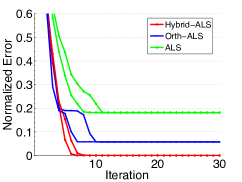
(a) $k=30,d=100$,
    uniform weights

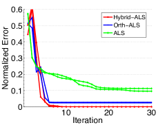
(b) $k=30,d=100$,
   $\frac{w_{\max}}{w_{\min}}=100$

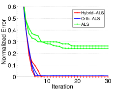
(c) $k=100,d=1000$,
   uniform weights

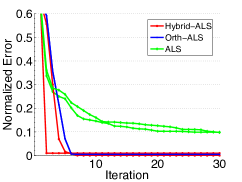
(d) $k=100,d=1000$,
   $\frac{w_{\max}}{w_{\min}}=100$

Figure 1: Plot of the normalized discrepancy between the recovered rank $k$ tensor $\hat{T}$ and the true tensor $T$: $\frac{\parallel T-\hat{T}\parallel_{\text{F}}}{\parallel T\parallel_{\text{F}}},$ as a function of the number of iterations. In all four settings, the Orth-ALS and the hybrid algorithms drive this discrepancy nearly to zero, with the performance of Orth-ALS improving for the higher dimensional cases, whereas the standard ALS algorithm has slower convergence and gets stuck in bad local optima.

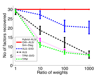
(a) Noiseless case, ratio of weights equals $\frac{w_{\max}}{w_{\min}}$

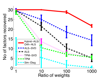
(b) Noisy case, ratio of weights equals $\frac{w_{\max}}{w_{\min}}$

Figure 2: Average number of factors recovered by different algorithms for different values of $\frac{w_{\max}}{w_{\min}}$, the ratio of the maximum factor weight to minimum factor weight (with the weights spaced geometrically), along with error bars for the standard deviation in the number of factors recovered, across independent trials. The true rank $k=30$, and the dimension $d=100$. We say a factor $\{A_{i},B_{i},C_{i}\}$ of the tensor $T$ is successfully recovered if there exists at least one recovered factor $\{\hat{A}_{j},\hat{B}_{j},\hat{C}_{j}\}$ with correlation at least 0.9 in all modes. Orth-ALS and Hybrid-ALS recover all factors in almost all settings, whereas ALS and the tensor power method struggle when the weights are skewed, even with the more expensive SVD based initialization.

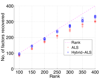
(a) No. of factors recovered for a dimension $d=50$ tensor with varying rank. The weights of the factors are geometrically spaced and the ratio of the weights between every pair of consecutive factors is 1.05

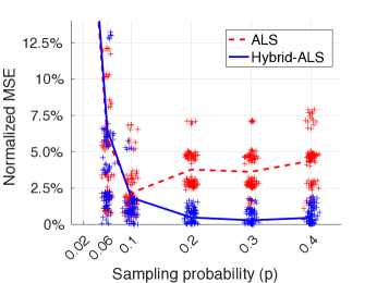
(b) Average error on the missing entries for tensor completion where each entry is sampled with probability $p$, on a 100 different runs with each setting of $p$. The tensor has dimension $d=50$ and rank $k=10$.

Figure 3: Experiments on overcomplete tensors and tensor completion. Even though our theoretical guarantees do not apply to these settings, we see that orthogonalization leads to significantly better performance over standard ALS.

Recovering over-complete tensors: Overcomplete tensors are tensors with rank higher than the dimension, and have found numerous theoretical applications in learning latent variable models Anandkumar et al. (2015). Even though orthogonalization cannot be directly applied to the setting where the rank is more than the dimension (as the factors can no longer be orthogonalized), we explore a deflation based approach in this setting. Given a tensor $T$ with dimension $d=50$ and rank $r>d$, we find a rank $d$ decomposition $T_{1}$ of $T$, subtract $T_{1}$ from $T$, and then compute a rank $d$ decomposition of $T_{1}$ to recover the next set of $d$ factors. We repeat this process to recover subsequent factors. After every set of $d$ factors has been estimated, we also refine the factor estimates of all factors estimated so far by running an additional ALS step using the current estimates of the extracted factors as the initialization. Fig. 3(a) plots the number of factors recovered when this deflation based approach is applied to a dimension $d=50$ tensor with a mild power low distribution on weights. We can see that Hybrid-ALS is successful at recovering tensors even in the overcomplete setup, and gives an improvement over ALS.

Tensor completion: We also test the utility of orthogonalization on a tensor completion task, where the goal is to recover a large missing fraction of the entries. Fig. 3(b) suggests Hybrid-ALS gives considerable improvements over standard ALS. Further examining the utility of orthogonalization in this important setting, in theory and practice, would be an interesting direction.

5.2 Learning Word Embeddings via Tensor Factorization

Algorithm	WordSim	MEN	Mixed analogies	Syntactic analogies
Vanilla ALS, $w=3$	0.47	0.51	30.22%	32.01%
Vanilla ALS, $w=5$	0.44	0.51	37.46%	37.27%
Orth-ALS, $w=3$	0.57	0.59	38.44%	42.40%
Orth-ALS, $w=5$	0.56	0.60	45.87%	47.13%
Matrix SVD, $w=3$	0.61	0.69	47.77%	61.79%
Matrix SVD, $w=5$	0.59	0.68	54.29%	62.20%

Table 1: Results for word analogy (mixed analogies and syntactic analogies) and word similarity tasks (WordSim, MEN) for different window lengths $w$ over which the co-occurrences are counted. The embeddings recovered by Orth-ALS are significantly better than those recovered by standard ALS. Despite this, embeddings derived from word co-occurrences using matrix SVD still outperform the tensor embeddings, and we are unsure whether this is due to the relative sparsity of the tensor, sub-optimal element-wise scaling (i.e. the $f(x)=\log(1+x)$ function applied to the co/tri-occurrence counts), or something more fundamental.

A word embedding is a vector representation of words which preserves some of the syntactic and semantic relationships in the language. Current methods for learning word embeddings implicitly Mikolov et al. (2013b); Levy and Goldberg (2014) or explicitly Pennington et al. (2014) factorize some matrix derived from the matrix of word co-occurrences $M$, where $M_{ij}$ denotes how often word $i$ appears with word $j$. We explore tensor methods for learning word embeddings, and contrast the performance of standard ALS and Orthogonalized ALS on standard tasks.

Methodology.

We used the English Wikipedia as our corpus, with 1.5 billion words. We constructed a word co-occurrence tensor $T$ of the 10,000 most frequent words, where the entry $T_{ijk}$ denotes the number of times the words $i$, $j$ and $k$ appear in a sliding window of length $w$ across the corpus. We consider two different window lengths, $w=3$ and $w=5$. Before factoring the tensor, we apply the non-linear element-wise scaling $f(x)=\log(1+x)$ to the tensor. This scaling is known to perform well in practice for co-occurrence matrices Pennington et al. (2014), and makes some intuitive sense in light of the Zipfian distribution of word frequencies. Following the application of this element-wise nonlinearity, we recover a rank 100 approximation of the tensor using Orth-ALS or ALS.

We concatenate the (three) recovered factor matrices into one matrix and normalize the rows. The $i$th row of this matrix is then the embedding for the $i$th word. We test the quality of these embeddings on two tasks aimed at measuring the syntactic and semantic structure captured by these word embeddings.

We also evaluated the performance of matrix SVD based methods on the task. For this, we built the co-occurrence matrix $M$ with a sliding window of length $w$ over the corpus. We applied the same non-linear element-wise scaling and performed a rank 100 SVD, and set the word embeddings to be the singular vectors after row normalization.

It is worth highlighting some implementation details for our experiments, as they indicate the practical efficiency and scalability inherited by Orth-ALS from standard ALS. Our experiments were run on a cluster with 8 cores and 48 GB of RAM memory per core. Most of the runtime was spent in reading the tensor, the runtime for Orth-ALS was around 80 minutes, with 60 minutes spent in reading the tensor (the runtime for standard ALS was around 100 minutes because it took longer to converge). Since storing a dense representation of the 10,000$\times$10,000$\times$10,000 tensor is too expensive, we use an optimized ALS solver for sparse tensors Smith and Karypis ; Smith and Karypis (2015) which also has an efficient parallel implementation.

Evaluation: Similarity and Analogy Tasks.

We evaluated the quality of the recovered word embeddings produced by the various methods via their performance on two different NLP tasks for which standard, human-labeled data exists: estimating the similarity between a pair of words, and completing word analogies.

The word similarity tasks Bruni et al. (2012); Finkelstein et al. (2001) contain word pairs along with human assigned similarity scores, and the objective is to maximize the correlation between the similarity in the embeddings of the two words (according to a similarity metric such as the dot product) and human judged similarity.

The word analogy tasks Mikolov et al. (2013a; c) present questions of the form “$a$ is to $a^{*}$ as $b$ is to  ?” (e.g. “Paris is to France as Rome is to  ?”). We find the answer to “$a$ is to $a^{*}$ as $b$ is to $b^{*}$” by finding the word whose embedding is the closest to $w_{a^{*}}-w_{a}+w_{b}$ in cosine similarity, where $w_{a}$ denotes the embedding of the word $a$.

Results.

The performances are summarized in the Table 1. The use of Orth-ALS rather than standard ALS leads to significant improvement in the quality of the embeddings as judged by the similarity and analogy tasks. However, the matrix SVD method still outperforms the tensor based methods. We believe that it is possible that better tensor based approaches (e.g. using better renormalization, additional data, or some other tensor rather than the symmetric tri-occurrence tensor) or a combination of tensor and matrix based methods can actually improve the quality of word embeddings, and is an interesting research direction. Alternatively, it is possible that natural language does not contain sufficiently rich higher-order dependencies among words that appear close together, beyond the co-occurrence structure, to truly leverage the power of tensor methods. Or, perhaps, the two tasks we evaluated on—similarity and analogy tasks—do not require this higher order. In any case, investigating these possibilities seems worthwhile.

6 Proof Overview: the Orthogonal Tensor Case

In this section, we will consider Orthogonalized ALS for the special case when the factors matrix of the tensor is an orthogonal matrix. Although this special case is easy and numerous algorithms provably work in this setting, it will serve to highlight the high level analysis approach that we apply to the more general settings.

The analysis of Orth-ALS hinges on an analysis of the tensor power method. For completeness we describe the tensor power method in Algorithm 2. We will go through some preliminaries for our analysis of the tensor power method. Let the iterate of the tensor power method at time $t$ be $Z_{t}$. The tensor power method update equations can be written as (refer to Anandkumar et al. (2014c))

$$Z_{t}=\frac{\sum_{i=1}^{k}w_{i}\langle Z_{t-1},A_{i}\rangle^{2}A_{i}}{{\parallel\sum_{i=1}^{k}w_{i}\langle Z_{t-1},A_{i}\rangle^{2}A_{i}\parallel_{2}}}$$ (6.1)

Eq. 6.1 is just the tensor analog of the matrix power method updates. For tensors, the updates are quadratic in the previous inner products, in contrast to matrices where the updates are linear in the inner products in the previous step.

Algorithm 2 Tensor power method to recover all factors Anandkumar et al. (2014c)

Input: Tensor $T\in\mathbb{R}^{d\times d\times d}$, number of initializations $L$, number of iterations $N$.

1:  for $\tau=1:L$ do

2:     Initialize $x_{0}^{(\tau)},y_{0}^{(\tau)},z_{0}^{(\tau)}\in\mathbb{R}^{d}$ uniformly from the unit sphere or using the SVD based method

3:     for $t=1:N$ do

4:        Rank-1 ALS/Power method updates-$x_{t+1}^{(\tau)}=T_{(1)}(\hat{z}_{t}^{(\tau)}\odot\hat{y}_{t}^{(\tau)})$

5:        Rank-1 ALS/Power method updates-$y_{t+1}^{(\tau)}=T_{(2)}(\hat{z}_{t}^{(\tau)}\odot\hat{x}_{t}^{(\tau)})$

6:        Rank-1 ALS/Power method updates-$z_{t+1}^{(\tau)}=T_{(3)}(\hat{y}_{t}^{(\tau)}\odot\hat{x}_{t}^{(\tau)})$

7:        Normalize $x_{t+1}^{\tau},y_{t+1}^{\tau},z_{t+1}^{\tau}$ and store results in $\hat{x}_{t+1}^{\tau},\hat{y}_{t+1}^{\tau},\hat{z}_{t+1}^{\tau}$.

8:     end for

9:     Estimate weights-$\hat{w}^{(\tau)}=T(\hat{x}_{N}^{(\tau)},\hat{y}_{N}^{(\tau)},\hat{z}_{N}^{(\tau)})$

10:  end for

11:  Cluster set $\{(\hat{w}^{(\tau)},\hat{x}_{N}^{(\tau)},\hat{y}_{N}^{(\tau)},\hat{z}_{N}^{(\tau)}),\tau\in[L]\}$ into $k$ clusters.

12:  return the centers $\{(\hat{w}_{i},\hat{a}_{i},\hat{b}_{i},\hat{c}_{i}),i\in[k]\}$ of the $k$ clusters as the estimates

Observe from Algorithm 1 (Orth-ALS) that the ALS steps in step 4-6 have the same form as tensor power method updates, but on the orthogonalized factors. This is the key idea we use in our analysis of Orth-ALS. Note that the first factor estimate is never affected by the orthogonalization, hence the updates for the first estimated factor have exactly the same form as the tensor power method updates, as this factor is unaffected by orthogonalization. The subsequent factors have an orthogonalization step before every tensor power method step. This ensures that they never have high correlation with the factors which have already been recovered, as they are projected orthogonal to the recovered factors before each ALS step. We then use the incoherence of the factors to argue that orthogonalization does not significantly affect the updates of the factors which have not been recovered so far, while ensuring that the factors which have already been recovered always have a small correlation.

Note that Eq. 6.1 is invariant with respect to multiplying the weights of all the factors by some constant. Hence for ease of exposition, we assume that all the weights lie in the interval $[1,\gamma]$, where $\gamma=\frac{w_{\max}}{w_{\min}}$. We also define $\eta=\max\{c_{\max},1/d\}$.

Proposition 1.

Consider a $d$-dimensional rank $k$ tensor $T=\sum_{i=1}^{k}w_{i}A_{i}\otimes A_{i}\otimes A_{i}$ where the factor matrix $A$ is orthogonal. Define $\gamma=\frac{w_{\max}}{w_{\min}}$ to be the ratio of the largest and smallest weight. If the initial estimates for all the factors are initialized randomly from the unit sphere and the factors $\{A_{j},j\geq i+1\}$ are re-randomized after $i(\log k+\log\log d)$ steps where $i$ is an integer, then with high probability the orthogonalized ALS updates converge to the true factors in $O(k(\log k+\log\log d))$ steps, and the error at convergence satisfies $\parallel A_{i}-\hat{A}_{i}\parallel_{2}^{2}\leq O(\gamma k/d^{2}\})$ and $|1-\frac{\hat{w}_{i}}{w_{i}}|\leq O(1/d)$ for all $i$.

Proof.

Without loss of generality, we assume that the $i$th recovered factor converges to the $i$th true factor. As mentioned earlier, the iterations for the first factor are the usual tensor power method updates and are unaffected by the remaining factors. Therefore to show that orthogonalized ALS recovers the first factor, we only need to analyze the tensor method updates. We show that the tensor power method with random initialization converges in $O(\log k+\log\log d)$ steps with probability at least ${(1-1/k^{1+\epsilon})}$, for any $\epsilon>0$. Hence this implies that Orth-ALS correctly recovers the first factor in $O(\log k+\log\log d)$ steps with probability at least $(1-1/k^{1+\epsilon})$, for any $\epsilon>0$.

The main idea of our proof of convergence of the tensor power method is the following – with decent probability, there is some separation between the correlations of the factors with the random initialization. By the tensor power method updates (Eq. 6.1), this gap is amplified at every stage. We analyze the updates for all the factors together by a simple recursion. We then show that this recursion converges in in $O(\log k+\log\log d)$ steps.

Let $Z_{t}$ be the iterate of the tensor power method updates at time $t$. Without loss of generality, we will be proving convergence to the first factor $A_{1}$. Let $a_{i,t}$ be the correlation of the $i$th factor $A_{i}$ with $Z_{t}$, i.e. $a_{i,t}=\langle A_{i},Z_{t}\rangle$ (note that this should technically be called the inner product, but we refer to it as the correlation). We will refer to $w_{i}a_{i,t}$ as the weighted correlation of the $i$th factor.

The first step of the proof is that with decent probability, there is some separation between the weighted correlation of the factors with the initial random estimate. This is Lemma 1.

Lemma 1.

If $\gamma kc_{\max}\leq 1/k^{1+\epsilon}$ for some $\epsilon>0$, then with probability at least $\Big{(}1-\frac{\log^{5}k}{k^{1+\epsilon}}\Big{)}$, $\frac{|{w_{i}}a_{i,0}|}{\max_{i}|{w_{i}}a_{i,0}|}\leq{1-5/k^{1+\epsilon}}$ $\;\forall\;i\neq\operatorname*{arg\,max}_{i}|w_{i}a_{i,0}|$.

The proof of Lemma 1 is a bit technical, but relies on basic concentration inequalities for Gaussians. Then using Eq. 6.1 the correlation at the end of the $(t+1)$th time step is given by

$$a_{i,t+1} ={w_{i}a_{i,t}^{2}}/\kappa_{t}$$

where $\kappa_{t}={\parallel\sum_{i=1}^{k}w_{i}\langle Z_{t-1},A_{i}\rangle^{2}\parallel_{2}}$ is the normalizing factor at the $t$th time step.

Because the estimate is normalized at the end of the updates, we only care about the ratio of the correlations of the factors with the estimate rather than the magnitude of the correlations themselves. Hence, it is convenient to normalize all the correlations by the correlation of the largest factor and normalize all the weights by the weight of the largest factor. Therefore, let $\hat{a}_{i,t}=\frac{a_{i,t}}{a_{1,t}}$ and $\hat{w}_{i}=\frac{w_{i}}{w_{1}}$. The new update equation for the ratio of correlations $\hat{a}_{i,t}$ is-

$$\hat{a}_{i,t+1} ={\hat{w}_{i}\hat{a}_{i,t}^{2}}$$ (6.2)

Our goal is to show that $a_{i,t}$ becomes small for all $i\neq 1$ in $O(\log k+\log\log d)$ steps. Instead of separately analyzing the different $a_{i,t}$ for different factors $A_{i}$, we upper bound $a_{i,t}$ for all $i$ via a simple recursion. Consider the recursion,

$$\beta_{0} =\max_{i\neq 1}{\Big{|}\hat{w}_{i}\hat{a}_{i,0}\Big{|}}$$ (6.3)

$$\beta_{t+1} =\beta_{t}^{2}$$ (6.4)

We claim that $|\hat{w}_{i}\hat{a}_{i,t}|\leq\beta_{t}$ for all $t$ and $i\neq 1$. By Eq. 6.3, this is true for $t=0$ by definition. We prove our claim via induction. Assume that $|\hat{w}_{i}\hat{a}_{i,t}|\leq\beta_{t}$ for $t=p$. Note that by Eq. 6.2, $\hat{w}_{i}\hat{a}_{i,p+1}={\hat{w}_{i}^{2}\hat{a}_{i,p}^{2}}$. Therefore $w_{i}\hat{a}_{i,p+1}\leq\beta_{p+1}^{2}$ for all $i\neq 1$. Hence $|\hat{w}_{i}\hat{a}_{i,t}|\leq\beta_{t}$ for all $t$ and $i\neq 1$. Note that as the weights lie in the interval $[1,\gamma]$, $\hat{a}_{i,t}\leq\beta_{t}$.

To show convergence, we will now analyze the recursion in Eq. 6.3. We will show that $\beta_{t}$ becomes sufficiently small in $O(\log k+\log\log d)$ steps. Note that $\beta_{t}=(\beta_{0})^{2^{t}}$ and $\beta_{0}\leq 1-5/k^{1+\epsilon}$. Therefore $\beta_{t}\leq 0.1$ for $t=2\log k$. In another $\log\log d$ steps, $\beta_{t}\leq 1/d$. Hence $\beta_{t}\leq 1/d$ in $O(\log k+\log\log d)$ steps. As $\beta_{t}$ is an upper bound for the correlation of all but the first factor, hence $|\hat{a}_{i,t}|\leq 1/d$ for all $i\neq 1$ in $O(\log k+\log\log d)$ steps.

To finish the proof of convergence for the tensor power method, we need to show that the estimate $Z_{t}$ is close to $A_{1}$ if it has small correlation with every factor other than $A_{1}$. Lemma 2 shows that if the ratio of the correlation of every other factor with $A_{1}$ is small, then the residual $\ell_{2}$ error in estimating $A_{1}$ is also small.

Lemma 2.

Let $\gamma kc_{\max}\leq 1/k^{1+\epsilon}$. Without loss of generality assume convergence to the first factor $A_{1}$. Define $\hat{a}_{i,t}=|\frac{{a}_{i,t}}{{a}_{1,t}}|$- the ratio of the correlation of the $i$th and 1st factor with the iterate at time $t$. If $\hat{a}_{i,t}\leq 2\eta\;\forall\;i\neq 1$, then ${\parallel A_{1}-\hat{A}_{1}\parallel_{2}^{2}}\leq 10\gamma k\eta^{2}$ in the subsequent iteration. Also, if $\parallel A_{1}-\hat{A}_{1}\parallel_{2}^{2}\leq O(\gamma k\eta^{2})$ the relative error in the estimation of the weight $w_{1}$ is at most $O(\eta)$.

Using Lemma 2, it follows that the estimate $\hat{A}_{1}$ and $\hat{w}_{1}$ for the factor $A_{1}$ satisfies $\parallel A_{1}-\hat{A}_{1}\parallel_{2}^{2}\leq 10\gamma k/d^{2}$ and $|1-\frac{\hat{w}_{1}}{w_{1}}|\leq O(1/d)$. Hence we have shown that Orth-ALS correctly recovers the first factor.

We now prove that Orth-ALS also recovers the remaining factors. The proof proceeds by induction. We have already shown that the base case is correct and the algorithm recovers the first factor. We next show that if the first $(m-1)$ factors have converged, then the $m$th factor converges in $O(\log k+\log\log d)$ steps with failure probability at most $\tilde{O}(1/{k^{1+\epsilon}})$. The main idea is that as the factors have small correlation with each other, hence orthogonalization does not affect the factors which have not been recovered but ensures that the $m$th estimate never has high correlation with the factors which have already been recovered. Recall that we assume without loss of generality that the $i$th recovered factor $X_{i}$ converges to the $i$th true factor, hence $X_{i}=A_{i}+\hat{\Delta}_{i}$ for $i<m$, where ${\parallel\hat{\Delta}_{i}\parallel_{2}}\leq 10\gamma k/d^{2}$. This is our induction hypothesis, which is true for the base case as we just showed that the tensor power method updates converge with residual error at most $10\gamma k/d^{2}$.

Let $X_{m,t}$ denote the $m$th factor estimate at time $t$ and let $Y_{m}$ denote it’s value at convergence. We will first calculate the effect of the orthogonalization step on the correlation between the factors and the estimate $X_{m,t}$. Let $\{\bar{X}_{i},i<m\}$ denote an orthogonal basis for $\{X_{i},i<m\}$. The basis $\{\bar{X}_{i},i<m\}$ is calculated via QR decomposition, and can be recursively written down as follows,

$$\bar{X}_{i}=\frac{{X}_{i}-\sum_{j<i}\bar{X}_{j}^{T}X_{i}\bar{X}_{j}}{{\parallel{X}_{i}-\sum_{j<i}\bar{X}_{j}^{T}X_{i}\bar{X}_{j}\parallel_{2}}}$$ (6.5)

Note that the estimate $X_{m,t}$ is projected orthogonal to this basis. Define $\bar{X}_{m,t}$ as this orthogonal projection, which can be written down as follows –

$$\bar{X}_{m,t}=\bar{X}_{m,t}-\sum_{j<m}\bar{X}_{j}^{T}X_{m,t}\bar{X}_{j}$$

In the QR decomposition algorithm $\bar{X}_{m,t}$ is also normalized to have unit norm but we will ignore the normalization of $X_{m,t}$ in our analysis because as before we only consider ratios of correlations of the true factors with $\bar{X}_{m,t}$, which is unaffected by normalization.

We will now analyze the orthogonal basis $\{\bar{X}_{i},i<m\}$. The key idea is that the orthogonal basis $\{\bar{X}_{i},i<m\}$ is close to the original factors $\{A_{i},i<m\}$ as the factors are incoherent. Lemma 3 proves this claim.

Lemma 3.

Consider a stage of the Orthogonalized ALS iterations when the first $(m-1)$ factors have converged. Without loss of generality let $X_{i}=A_{i}+\hat{\Delta}_{i},i<m$, where${\parallel\hat{\Delta}_{i}\parallel_{2}}\leq 10\gamma k\eta^{2}$. Let $\{\bar{X}_{i},i<m\}$ denote an orthogonal basis for $\{X_{i},i<m\}$ calculated using Eq. 6.5. Then,

1. $\bar{X}_{i}=A_{i}+\Delta_{i},\;\forall\;i<m$ and ${\parallel\Delta_{j}\parallel_{2}}\leq 10k\eta$.

2. $|A_{j}^{T}\Delta_{i}|\leq 3\eta,\;\forall\;i<m,\;j<i$.

3. $|A_{j}^{T}\Delta_{i}|\leq 20\gamma k\eta^{2},\;\forall\;i<m,\;j>i$.

Using Lemma 3, we will find the effect of orthogonalization on the correlations of the factors with the iterate $X_{m,t}$. At a high level, we need to show that the iterations for the factors $\{A_{i},i\geq m\}$ are not much affected by the orthogonalization, while the correlations of the factors $\{A_{i},i<m\}$ with the estimate $X_{m,t}$ are ensured to be small. Lemma 3 is the key tool to prove this, as it shows that the orthogonalized basis is close to the true factors.

We will now analyze the inner product between $\bar{X}_{m,t}$ and factor $A_{i}$. This is given by-

$$A_{i}^{T}\bar{X}_{m,t}=A_{i}^{T}X_{m,t}-\sum_{j<m}X_{m,t}^{T}\bar{X}_{j}A_{i}^{T}\bar{X}_{j}$$

As earlier, we normalize all the correlations by the correlation of the largest factor, let $\bar{a}_{i,t}$ be the ratio of the correlations of $A_{i}$ and $A_{m}$ with the orthogonalized estimate $\bar{X}_{m,t}$ at time $t$. We can write $\bar{a}_{i,t}$ as-

$$\bar{a}_{i,t}=\frac{A_{i}^{T}X_{m,t}-\sum_{j<m}X_{m,t}^{T}\bar{X}_{j}A_{i}^{T}\bar{X}_{j}}{A_{m}^{T}X_{m,t}-\sum_{j<m}X_{m,t}^{T}\bar{X}_{j}A_{m}^{T}\bar{X}_{j}}$$

We can multiply both sides by $\hat{w}_{i}$ and substitute $\bar{X}_{j}$ from Lemma 3 and then rewrite as follows-

$$\hat{w}_{i}\bar{a}_{i,t}=\frac{\hat{w}_{i}A_{i}^{T}X_{m,t}-\sum_{j<m}\hat{w}_{i}X_{m,t}^{T}(A_{j}+\Delta_{j})A_{i}^{T}\Delta_{j}}{A_{m}^{T}X_{m,t}-\sum_{j<m}X_{m,t}^{T}(A_{j}+\Delta_{j})A_{m}^{T}\Delta_{j}}$$

We divide the numerator and denominator by $A_{m}^{T}X_{m,t}$ to derive an expression in terms of the ratios of correlations. Let $\delta_{i,t}=\frac{X_{m,t}^{T}\Delta_{j}}{X_{m,t}^{T}A_{m}}$.

$$\hat{w}_{i}\bar{a}_{i,t}=\frac{\hat{w}_{i}\hat{a}_{i,t}-\sum_{j<m}(\hat{w}_{i}\hat{a}_{j,t}+\hat{w}_{i}\delta_{i,t})A_{i}^{T}\Delta_{j}}{1-\sum_{j<m}(\hat{a}_{j,t}+\delta_{i,t})A_{m}^{T}\Delta_{j}}$$

We now need to show $\hat{w}_{i}\bar{a}_{i,t}$ is small for all $i<m$ and is close to $\hat{w}_{i}{a}_{i,t}$, the weighted correlation before orthogonalization, for all $i>m$. Lemma 4 proves this, and shows that the weighted correlation of factors which have not yet been recovered, $\{A_{i},i\geq m\}$, is not much affected by orthogonalization, but the factors which have already been recovered. $\{A_{i},i<m\}$, are ensured to be small after the orthogonalization step.

Lemma 4.

Let $|\hat{w}_{i}\hat{a}_{i,t}|\leq\beta_{t}\;\forall\;i\neq m$ at the end of the $t$th iteration. Let $\bar{a}_{i,t}$ be the ratio of the correlation of the $i$th and the $m$th factor with $X_{m,t}$, the iterate at time $t$ after the orthogonalization step. Then,

1. $|\hat{w}_{i}\bar{a}_{i,t}|\leq\beta_{t}(1+1/k^{1+\epsilon})),\;\forall\;i>m$.

2. $|\hat{w}_{i}\bar{a}_{i,t}|\leq 50\gamma k\eta\beta_{t},\;\forall\;i<m$.

We are now ready to analyze the Orth-ALS updates for the $m$th factor. First, we argue about the initialization step. Lemma 4 shows that an orthogonalization step performed after a random initialization ensures that the factors which have already been recovered have small correlation with the orthogonalized initialization. This is where we need a periodic re-randomization of the factors which have not converged so far.

Lemma 5.

Let $X_{m,0}$ be initialized randomly and the result be projected orthogonal to the $(m-1)$ previously estimated factors, let these be $\{X_{i},i<m\}$ without loss of generality. Then $\operatorname*{arg\,max}_{i}|w_{i}a_{i,0}|\geq m$ with high probability. Also, with failure probability at most $\Big{(}1-\frac{\log^{5}k}{k^{1+\epsilon}}\Big{)}$, $\Big{|}\frac{w_{i}\bar{a}_{i,0}}{\max_{i}\{w_{i}\bar{a}_{i,0}\}}\Big{|}\leq{1-4/k^{1+\epsilon}}\;\forall\;i\neq\operatorname*{arg\,max}_{i}|w_{i}a_{i,0}|$ after the orthogonalization step.

Lemma 5 shows that with high probability, the initialization for the $m$th recovered factor has the largest weighted correlation with a factor which has not been recovered so far after the orthogonalization step. It also shows that the separation condition in Lemma 1 is satisfied for all remaining factors with probability $(1-\log^{5}k/k^{1+\epsilon})$.

Now, we combine the effects of the tensor power method step and the orthogonalization step for subsequent iterations to show that that $X_{m,t}$ converges to $A_{m}$. Consider a tensor power method step followed by an orthogonalization step. By our previous argument about the convergence of the tensor power method, if $|\hat{w}_{i}\hat{a}_{i,t-1}|\leq\beta_{t-1}$ $i\neq m$ at some time $(t-1)$, then $|\hat{w}_{i}\hat{a}_{i,t}|\leq\beta_{t-1}^{2}$ for $i\neq m$ after a tensor power method step. Lemma 4 shows that the correlation of all factors other than the $m$th factor is still small after the orthogonalization step, if it was small before. Combining the effect of the orthogonalization step via Lemma 4, if $|\hat{w}_{i}\hat{a}_{i,t-1}|\leq\beta_{t-1}$ $i\neq m$ for some time $(t-1)$, then $|\hat{w}_{i}\hat{a}_{i,t}|\leq\beta_{t-1}^{2}(1+1/k^{1+\epsilon})$ for $i\neq m$ after both the tensor power method and the orthogonalization steps. By also using Lemma 5 for the initialization, can now write the updated combined recursion analogous to Eq. 6.3 and Eq. 6.4, but which combines the effect of the tensor power method step and the orthogonalization step.

$$\beta_{0} =\max_{i\neq 1}{\Big{|}\hat{w}_{i}\hat{a}_{i,0}\Big{|}}$$ (6.6)

$$\beta_{t+1} =\beta_{t}^{2}(1+1/k^{1+\epsilon})$$ (6.7)

By the previous argument, $|w_{i}\bar{a}_{i,t}|\leq\beta_{t}$. Note that $\beta_{0}\leq 1-4/k^{1+\epsilon}$ by Lemma 5. By expanding the recursion 6.7, $\beta_{t}=(\beta_{0}(1+1/k^{1+\epsilon}))^{2^{t}}$. Hence $\beta_{t}\leq 1/d$ in $2\log k+\log\log d$ steps as was the case for the analysis for the tensor power method. This shows that the correlation of the estimate $X_{m,t}$ with all factors other than $A_{m}$ becomes small in $2\log k+\log\log d$. We now again use Lemma 2 to argue that this implies that the recovery error is small, i.e. $\parallel A_{m}-\hat{A}_{m}\parallel_{2}^{2}\leq 10\gamma k/d^{2}$ and $|1-\frac{\hat{w}_{m}}{w_{m}}|\leq O(1/d)$.

Hence we have shown that if the first $(m-1)$ factors have converged to $X_{i}=A_{i}+\hat{\Delta}_{i}$ where ${\parallel\hat{\Delta}_{i}\parallel_{2}}\leq 10\gamma k/d^{2},\;\forall\;i<m$ then the $m$th factor converges to $X_{m}=A_{m}+\hat{\Delta}_{m}$ where ${\parallel\hat{\Delta}_{m}\parallel_{2}}\leq 10\gamma k/d^{2}$ in $O(\log k+\log\log d)$ steps with probability at least $\Big{(}1-\frac{\log^{5}k}{k^{1+\epsilon}}\Big{)}$. This proves the induction hypothesis.

We can now do a union bound to argue that each factor converges with $\ell_{2}$ error at most $O(\gamma k/d^{2})$ in $O(k(\log k+\log\log d))$ with overall failure probability at most $\tilde{O}(1/k^{-\epsilon}),\epsilon>0$. This finishes the proof of convergence of Orth-ALS for the special case of orthogonal tensors.

∎

7 Conclusion

Our results suggest the theoretical and practical benefits of Orthogonalized ALS, versus standard ALS. An interesting direction for future work would be to more thoroughly examine the practical and theoretical utility of orthogonalization for other tensor-related tasks, such as tensor completion. Additionally, its seems worthwhile to investigate Orthogonalized ALS or Hybrid ALS in more application-specific domains, such as natural language processing.

Appendix A Global convergence of the tensor power method for incoherent tensors

In this section, we will analyze the tensor power method updates for worst-case incoherent tensors. This is a necessary step before analyzing Orth-ALS, because as was pointed out in the proof of convergence of Orth-ALS in the orthogonal tensor case, analyzing Orth-ALS updates reduces to analyzing a perturbed version of the tensor power method updates. Our convergence results for the tensor power method are interesting independent of Orth-ALS though, as they prove global convergence under random initialization. The proof idea is similar to the proof of convergence of the tensor power method in the orthogonal case, but we now need to analyze the cross-terms which come in because the factors are no longer orthogonal.

See 3

Proof.

Without loss of generality, we will prove convergence to the first factor $A_{1}$. The proof is similar in spirit to the proof of convergence of the tensor power method in the orthogonal case in Section 6.

As in the orthogonal case, Lemma 1 states that with high probability there is some separation between the weighted correlation of the largest and second largest factors. See 1

We normalize all the correlations by the correlation of the largest factor, let $\hat{a}_{i,t+1}=\frac{a_{i,t}}{a_{1,t}}$ and normalize all the weights by the weight of the largest factor, $\hat{w}_{i}=\frac{w_{i}}{w_{1}}$. The new update equations in terms of the ratio of correlations $\hat{a}_{i,t}$ become-

$$\hat{a}_{i,t+1} =\frac{\hat{w}_{i}\hat{a}_{i,t}^{2}+c_{i,1}+\sum_{j:j\neq\{i,1\}}c_{i,j}\hat{w}_{j}\hat{a}_{j,t}^{2}}{1+\sum_{j:j\neq 1}c_{1,j}\hat{w}_{j}\hat{a}_{j,t}^{2}}$$ (A.1)

Notice that we have cross terms in Eq. A.1 as compared to Eq. 6.2 in the orthogonal case, due to the correlation $c_{i,j}$ between the factors being non-zero. The goal of the analysis for the non-orthogonal case is to bound these cross-terms using the incoherence between the factors.

As in the orthogonal case, we will analyze all the correlations $\hat{a}_{i,t}$ via a single recursion. We define $\beta_{t}$ in the non-orthogonal case keeping in mind the cross-terms because of the correlations between the factors being non-zero.

$$\beta_{0} =\max_{i\neq 1}{\Big{|}{w_{i}}\hat{a}_{i,0}\Big{|}}$$ (A.2)

$$\beta_{t+1} =\gamma c_{\max}+\beta_{t}^{2}+3\gamma kc_{\max}\beta_{t}^{2}$$ (A.3)

We now show that $|{w_{i}}\hat{a}_{i,t}|\leq\beta_{t},\forall\;i\neq 1$ and all $t$.

Lemma 6.

If $|\hat{w}_{i}\hat{a}_{i,m}|\leq\beta_{m}$ for some time $m$ and for all $i\neq 1$, then at time $(m+1)$ for all $i\neq 1$,

1. $|\hat{w}_{i}\hat{a}_{i,m+1}|\leq\beta_{m+1}$.

2. $|\hat{a}_{i,m+1}-c_{i,1}|\leq 2\beta_{m}^{2}$

Proof.

Note that by Lemma 7, $\beta_{t}<1\;\forall\;t\implies\hat{w}_{i}\hat{a}_{i,m}^{2}\leq 1$. Therefore $\sum_{j}|c_{i,j}\hat{w}_{j}\hat{a}_{j,m}^{2}|\leq kc_{\max}\leq 1/k^{1+\epsilon}\;\forall\;i$. Hence we can write,

$$\frac{1}{1+\sum_{j:j\neq 1}c_{1,j}\hat{w}_{j}\hat{a}_{j,m}^{2}}=1-\sum_{j:j\neq 1}c_{1,j}\hat{w}_{j}\hat{a}_{j,m}^{2}+\epsilon_{1}$$

where $\epsilon_{1}$ is the residual term, and $|\epsilon_{1}|\leq\Big{|}\sum_{j:j\neq 1}c_{1,j}\hat{w}_{j}\hat{a}_{j,m}^{2}\Big{|}^{2}\leq k^{2}c_{\max}^{2}\leq 1/k^{2}$. We can now rewrite the updates for $\hat{a}_{i,m+1}$ as-

$$\hat{a}_{i,m+1} =\Big{(}c_{i,1}+\hat{w}_{i}\hat{a}_{i,m}^{2}+\sum_{j:j\neq\{i,1\}}c_{i,j}\hat{w}_{j}\hat{a}_{j,m}^{2}\Big{)}\Big{(}1-\sum_{j:j\neq 1}c_{1,j}\hat{w}_{j}\hat{a}_{j,m}^{2}+\epsilon_{1}\Big{)}$$

Let $\rho_{i,m}=c_{i,1}+\hat{w}_{i}\hat{a}_{i,m}^{2}+\sum_{j:j\neq\{i,1\}}c_{i,j}\hat{w}_{j}\hat{a}_{j,m}^{2}$. We can write,

$$\hat{a}_{i,m+1} =c_{i,1}+\hat{w}_{i}\hat{a}_{i,m}^{2}+\sum_{j:j\neq\{i,1\}}c_{i,j}\hat{w}_{j}\hat{a}_{j,m}^{2}-\rho_{i,m}\sum_{j:j\neq 1}c_{1,j}\hat{w}_{j}\hat{a}_{j,m}^{2}+\rho_{i,m}\epsilon_{1}$$ (A.4)

$$\implies\Big{|}\hat{a}_{i,m+1}\Big{|} \leq\Big{|}c_{i,1}\Big{|}+\Big{|}\hat{w}_{i}\hat{a}_{i,m}^{2}\Big{|}+\Big{|}\sum_{j:j\neq\{i,1\}}c_{i,j}\hat{w}_{j}\hat{a}_{j,m}^{2}\Big{|}+\Big{|}\rho_{i,m}\sum_{j:j\neq 1}c_{1,j}\hat{w}_{j}\hat{a}_{j,m}^{2}\Big{|}+\Big{|}\rho_{i,m}\epsilon_{1}\Big{|}$$ (A.5)

We claim that $\rho_{i,m}\leq 1$. We verify this as follows,

$$\rho_{i,m} =c_{i,1}+\hat{w}_{i}\hat{a}_{i,m}^{2}+\sum_{j:j\neq\{i,1\}}c_{i,j}\hat{w}_{j}\hat{a}_{j,m}^{2}$$

$$\implies\Big{|}\rho_{i,m}\Big{|} \leq\Big{|}c_{i,1}\Big{|}+\Big{|}\hat{w}_{i}\hat{a}_{i,m}^{2}\Big{|}+\Big{|}\sum_{j:j\neq\{i,1\}}c_{i,j}\hat{w}_{j}\hat{a}_{j,m}^{2}\Big{|}$$

$$\implies\Big{|}\hat{w}_{i}\rho_{i,m}\Big{|} \leq\gamma\Big{|}c_{i,1}\Big{|}+\Big{|}\hat{w}_{i}^{2}\hat{a}_{i,m}^{2}\Big{|}+\Big{|}\sum_{j:j\neq\{i,1\}}c_{i,j}\hat{w}_{i}\hat{w}_{j}\hat{a}_{j,m}^{2}\Big{|}$$

$$\leq\gamma c_{\max}+\beta_{m}^{2}+\gamma kc_{\max}\beta_{m}^{2}$$

$$\leq\beta_{m+1}\leq 1$$

$$\implies\Big{|}\rho_{i,m}\Big{|} \leq 1$$

where we used the fact that the weights lie in the interval $[1,\gamma]$. Hence $|\rho_{i,m}|\leq 1$. Therefore, by Eq. A.5,

$$\Big{|}\hat{a}_{i,m+1}\Big{|} \leq\Big{|}c_{i,1}\Big{|}+\Big{|}\hat{w}_{i}\hat{a}_{i,m}^{2}\Big{|}+\Big{|}\sum_{j:j\neq\{i,1\}}c_{i,j}\hat{w}_{j}\hat{a}_{j,m}^{2}\Big{|}+\Big{|}\sum_{j:j\neq 1}c_{1,j}\hat{w}_{j}\hat{a}_{j,m}^{2}\Big{|}+\Big{|}\epsilon_{1}\Big{|}$$

$$\implies\Big{|}\hat{w}_{i}\hat{a}_{i,m+1}\Big{|} \leq\gamma\Big{|}c_{i,1}\Big{|}+\Big{|}\hat{w}_{i}^{2}\hat{a}_{i,m}^{2}\Big{|}+\Big{|}\sum_{j:j\neq\{i,1\}}c_{i,j}\hat{w}_{i}\hat{w}_{j}\hat{a}_{j,m}^{2}\Big{|}+\Big{|}\sum_{j:j\neq 1}c_{1,j}\hat{w}_{i}\hat{w}_{j}\hat{a}_{j,m}^{2}\Big{|}+\gamma\Big{|}\epsilon_{1}\Big{|}$$

$$\leq\gamma c_{\max}+\beta_{m}^{2}+3\gamma kc_{\max}\beta_{m}^{2}=\beta_{m+1}$$ (A.6)

To show that $|\hat{a}_{i,m+1}-c_{i,1}|\leq 2\beta_{m}^{2}$ we use Eq. A.4 and repeat the steps used to show that $|\hat{w}_{i}\hat{a}_{i,m+1}|\leq\beta_{m+1}\;\forall\;t$. ∎

By using induction and Lemma 6, the iterates at all time $t$ satisfy the following properties, for all $i\neq 1$,

1. $|\hat{w}_{i}\hat{a}_{i,t}|\leq\beta_{t}\;\forall\;t$.

2. $|\hat{a}_{i,t}-c_{i,1}|\leq 2\beta_{t-1}^{2}$

This allows us to analyze the iterations of $\beta_{t}$ instead of keeping track of the different $a_{i,t}$. We will now analyze the recursion for $\beta_{t}$. The following Lemma shows that $\beta_{t}$ becomes sufficiently small in $O(\log k+\log\log d)$ steps.

Lemma 7.

$\beta_{t}\leq 3\gamma\eta\;\forall\;t\geq O(\log k+\log\log d)$, also $\beta_{t}<1\;\forall\;t$

Proof.

We divide the updates into three stages.

1. $0.1\leq\beta_{t}\leq{1-5/k^{1+\epsilon}}$:

   As $\beta_{t}\geq 0.1$, therefore $k\beta_{t}^{2}\geq 1$ in this regime and hence $\gamma c_{\max}\leq\gamma kc_{\max}\beta_{t}^{2}$, and we can write-

   $$\beta_{t+1} =\gamma c_{\max}+\beta_{t}^{2}+3\gamma kc_{\max}\beta_{t}^{2}$$

   $$\beta_{t+1} \leq\beta_{t}^{2}+4\gamma kc_{\max}\beta_{t}^{2}$$

   We claim that $\beta_{t}<0.1$ for $t=O(\log d)$. To verify, note that-

   $$\beta_{t} \leq(\beta_{0}(1+4\gamma kc_{\max}))^{2^{t}}$$

   $$\leq\Big{(}(1-5/k^{1+\epsilon})(1+1/k^{1+\epsilon})\Big{)}^{2^{t}}$$

   $$\leq\Big{(}1-1/k^{1+\epsilon}\Big{)}^{2^{t}}$$ (A.7)

   where we used the fact that $\gamma kc_{\max}\leq 1/k^{1+\epsilon}$. Note that $(1-1/k^{1+\epsilon})^{2^{t}}\leq 0.1$ for $t=2\log k$ and hence we stay in this regime for at most $2\log k$ steps.

2. $\sqrt{\gamma\eta}\leq\beta_{t}\leq 0.1:$

   For notational convenience, we restart $t$ from 0 in this stage. Because $\gamma c_{\max}\leq\gamma\eta\leq\beta_{t}^{2}$ in this regime and $3\gamma kc_{\max}\beta_{t}^{2}\leq 0.1\beta_{t}^{2}$ as $\gamma kc_{\max}\leq 1/k^{1+\epsilon}$, we can write-

   $$\beta_{t+1} =\gamma c_{\max}+\beta_{t}^{2}+3\gamma kc_{\max}\beta_{t}^{2}$$

   $$\leq\beta_{t}^{2}+\beta_{t}^{2}+0.3\beta_{t}^{2}\leq 2.5\beta_{t}^{2}$$

   We claim that $\beta_{t}<\sqrt{\gamma\eta}$ for $t=O(\log\log\gamma\eta^{-1})$. To verify, note that-

   $$\beta_{t} \leq(2.5\beta_{t})^{2^{t}}\leq(0.25)^{2^{t}}$$ (A.8)

   Note that $(0.25)^{2^{t}}\leq\sqrt{\gamma\eta}$ for $t=O(\log\log(\gamma\eta)^{-1})$ and hence we stay in this stage for at most $O(\log\log(\gamma\eta)^{-1})$ steps. As $\eta^{-1}=O(d)$, this stage continues for at most $O(\log\log d)$ steps.

3. Note that in the next step, $\beta_{t}\leq\gamma c_{\max}+1.1\gamma\eta\leq 3\gamma\eta$. This is again because $3\gamma kc_{\max}\beta_{t}^{2}\leq 0.1\beta_{t}^{2}$and $\beta_{t}\leq\sqrt{\gamma\eta}$ at the end of the previous stage.

∎

Hence $\beta_{t}\leq 3\gamma\eta$ for $t=O(\log\log d+\log k)$. By Lemma 6, $|\hat{a}_{i,t}-c_{i,1}|\leq 18\gamma^{2}\eta^{2},i\neq 1$. Hence $|\hat{a}_{i,t}|\leq 2\eta$. By Lemma 2, the error at convergence satisfies ${\parallel A_{1}-\hat{A}_{1}\parallel_{2}}\leq 10\gamma k\eta^{2}$ and the estimate of the weight $\hat{w}_{1}$ satisfies $|1-\frac{\hat{w}_{1}}{w_{1}}|\leq O(\eta)$. ∎

Appendix B Global convergence of the tensor power method for random tensors

The previous section gives global convergence guarantees for the tensor power method for incoherent tensors. Applying Theorem 3 to a tensor whose factors are chosen uniformly at random, we can say that the tensor power method converges with random initialization whenever the rank $k=o(d^{0.25})$. Theorem 3 also proves a linear convergence rate. However, this is quite suboptimal for random tensors. In this section, we use the randomness in the tensor to get much stronger convergence results.

The techniques used in this section are very different from the rest of the paper. Instead of recursively analyzing the tensor power method updates by showing that the algorithm makes progress at every step by boosting its correlation with some fixed factor, we directly express the correlation of the factors with the estimate $Z_{\tau}$ after a fixed number of $\tau=O(\log\log d)$ time steps in terms of the initial correlations of the factors with the random initialization. This allows us to then skillfully use the randomness in the factors to get strong results. The difficulty with the recursive approach is that all the randomness in the tensor is “lost” after just one tensor power method update, i.e. the correlations of different factors with the estimate are no longer independent of each other, which makes the analysis much more difficult.

See 2

Proof.

Without loss of generality, we will prove convergence to the first factor $A_{1}$. Let $\tau=5\log\log d^{2}$. As before, define $a_{i,t}=\langle A_{i},Z_{t}\rangle$ where $Z_{t}$ is the iterate at time $t$. For the analysis of the tensor power method updates for random tensors we ignore the normalization step of the updates, till the last iteration. It is easy to see that this makes no difference in the analysis, though in practice it is important to normalize after every step to prevent the vectors from becoming too small and causing numerical errors. Recall that the update equations for ${a}_{i,t}$ for any $t$ are-

$${a}_{i,t} ={w}_{i}{a}_{i,t-1}^{2}+c_{i,1}w_{1}a_{1,t-1}^{2}+\sum_{j:j\neq\{i,1\}}c_{i,j}{w}_{j}{a}_{j,t-1}^{2}$$ (B.1)

and the iterate $X_{\tau+1}$ at time $\tau+1$ can be written as

$$Z_{\tau+1}={w}_{1}{a}_{1,\tau}^{2}A_{1}+\sum_{i\neq 1}{w}_{i}{a}_{i,\tau}^{2}A_{i}$$

On expanding $w_{1}{a}_{1,\tau}^{2}$ recursively using Eq. B.1, one of the terms that appears in the expansion is ${(w_{1}a_{1,0})^{2^{\tau}}}/{w_{1}}$. Define $\alpha_{\tau}={|w_{1}a_{1,0}|^{2^{\tau}}}/{w_{1}}$. Let $\Delta_{\tau}=(1/\alpha_{\tau})\sum_{i\neq 1}{w}_{i}{a}_{i,\tau}^{2}A_{i}$. We show that ${\parallel\Delta_{\tau}\parallel_{2}}\leq\tilde{O}(1/\sqrt{d})$ with failure probability at most $\log^{-1}d$. We can write $(1/\alpha_{\tau}){{w}_{1}{a}_{1,\tau}^{2}}$, the coefficient for first factor $A_{1}$ normalized by $\alpha_{\tau}$, as follows

$$\frac{{w}_{1}{a}_{1,\tau}^{2}}{\alpha_{\tau}} =\frac{(w_{1}a_{1,0})^{2^{\tau}}}{w_{1}\alpha_{\tau}}+\frac{1}{\alpha_{\tau}}\Big{(}w_{1}a_{1,\tau}^{2}-\frac{(w_{1}a_{1,0})^{2^{\tau}}}{w_{1}}\Big{)}$$

$$=1+\frac{1}{\alpha_{\tau}}\Big{(}w_{1}a_{1,\tau}^{2}-\frac{(w_{1}a_{1,0})^{2^{\tau}}}{w_{1}}\Big{)}$$

Let $\lambda_{\tau}=\frac{1}{\alpha_{\tau}}\Big{(}w_{1}a_{1,\tau}^{2}-\frac{(w_{1}a_{1,0})^{2^{\tau}}}{w_{1}}\Big{)}$. Let $Z_{\tau+1}^{\prime}=Z_{\tau+1}/\alpha_{\tau}$. We can write $Z_{\tau+1}^{\prime}$ as

$$Z_{\tau+1}^{\prime}=(1+\lambda_{\tau})A_{1}+\Delta_{\tau}$$

Note that $\frac{Z_{\tau+1}^{\prime}}{{\parallel Z_{\tau+1}^{\prime}\parallel_{2}}}=\frac{Z_{\tau+1}}{{\parallel Z_{\tau+1}\parallel_{2}}}$. Let $\frac{Z_{\tau+1}^{\prime}}{{\parallel Z_{\tau+1}^{\prime}\parallel_{2}}}=\tilde{Z}_{\tau+1}$. We desire to show that the residual ${\parallel\tilde{Z}_{\tau+1}-A_{1}\parallel_{2}}\leq\tilde{O}(1/\sqrt{d})$. We can bound ${\parallel\tilde{Z}_{\tau+1}-A_{1}\parallel_{2}}$ as follows using the triangle inequality,

$${\parallel\tilde{Z}_{\tau+1}-A_{1}\parallel_{2}}\leq\Big{|}\frac{1+\lambda_{\tau}}{{\parallel(1+\lambda_{\tau})A_{1}+\Delta_{\tau}\parallel_{2}}}-1\Big{|}+\frac{{\parallel\Delta_{\tau}\parallel_{2}}}{{\parallel(1+\lambda_{\tau})A_{1}+\Delta_{\tau}\parallel_{2}}}$$

If ${\parallel\Delta_{\tau}\parallel_{2}}\leq\tilde{O}(1/\sqrt{d})$ and $|\lambda_{\tau}|\leq d^{-\epsilon}$ then,

$${\parallel\tilde{Z}_{\tau+1}-A_{1}\parallel_{2}} \leq\Big{|}\frac{1}{{\parallel A_{1}+\Delta_{\tau}/(1+\lambda_{\tau})\parallel_{2}}}-1\Big{|}+\frac{{\parallel\Delta_{\tau}\parallel_{2}}}{1-|\lambda_{\tau}|-{\parallel\Delta_{\tau}\parallel_{2}}}$$

$$\leq\frac{2{\parallel\Delta_{\tau}\parallel_{2}}}{1-|\lambda_{\tau}|}+\frac{{\parallel\Delta_{\tau}\parallel_{2}}}{1-|\lambda_{\tau}|-{\parallel\Delta_{\tau}\parallel_{2}}}\leq\tilde{O}(1/\sqrt{d})$$

If ${\parallel\tilde{Z}_{\tau+1}-A_{1}\parallel_{2}}\leq\tilde{O}(1/\sqrt{d})$ then, by Lemma 2, the estimate of the weight $\hat{w}_{1}$ satisfies $|1-\frac{\hat{w}_{1}}{w_{1}}|\leq\tilde{O}(1/\sqrt{d})$.

Hence we will show that ${\parallel\Delta_{\tau}\parallel_{2}}\leq\tilde{O}(1/\sqrt{d})$ and $|\lambda_{\tau}|\leq d^{-\epsilon}$ with failure probability at most $\log^{-1}d$. Let $\epsilon_{\tau}={\parallel\Delta_{\tau}\parallel_{2}}^{2}$. We can write $\epsilon_{\tau}$ as

$$\epsilon_{\tau}={\parallel\Delta_{\tau}\parallel_{2}}^{2} =\sum_{i\neq 1,j\neq 1}(1/\alpha_{\tau}^{2}){w}_{i}w_{j}{a}_{i,\tau}^{2}{a}_{j,\tau}^{2}c_{i,j}$$

We can also write $\lambda_{\tau}^{2}$ as follows-

$$\lambda_{\tau}^{2}=(1/\alpha_{\tau}^{2})w_{1}^{2}\Big{(}a_{1,\tau}^{2}-\frac{(w_{1}a_{1,0})^{2^{\tau}}}{w_{1}^{2}}\Big{)}^{2}$$

Note that $\lambda_{\tau}$ has the same form as $\epsilon_{\tau}$ with the restriction that $i=j=1$ and the $\frac{(w_{1}a_{1,0})^{2^{\tau}}}{w_{1}^{2}}$ in the expansion of $a_{1,\tau}^{2}$ is removed.

Our approach will be to recursively expand the ${a}_{i,\tau}^{2}$ terms to express $\epsilon_{\tau}$ and $\lambda_{\tau}$ only in terms of $a_{i,0}$ (the initial correlations at time 0), the correlation between factors $c_{i,j}$ and the weights $w_{i}$. We use the recursion Eq. B.1 to do this.

We first consider the expansion of $a_{i,\tau}^{2}$ for any $i$ using recursion Eq. B.1. $a_{i,t}^{2}$ can be written as a weighted sum of correlations of the factors with the iterate at the $(t-1)$st time step as follows using recursion Eq. B.1-

$$a_{i,t}^{2} =\Big{(}w_{i}a_{i,t-1}^{2}+\sum_{j\neq i}c_{i,j}w_{j}a_{j,t-1}^{2}\Big{)}^{2}$$ (B.2)

$$=\sum_{j,k}w_{j}w_{k}c_{i,j}c_{i,k}a_{j,t-1}^{2}a_{k,t-1}^{2}$$ (B.3)

Each term in the summation corresponds to two choices for the terms at time $(t-1)$, the $j$ and $k$ variables. Continuing this recursive expansion for $\tau$ time steps, we can represent each monomial in the expansion by a complete binary tree with depth $\tau$. We label a node of the binary tree as $j$ if it corresponds to factor $A_{j}$. For ease of exposition, we will consider the initialization $Z_{0}$ as the 0th factor for the graph representation, hence $c_{i,0}=a_{i,0}$. The root of the tree is labeled as $i$ as it corresponds to the factor $A_{i}$. The descendants of the root $i$ are labelled as $j$ and $k$ if $a_{i,\tau}^{2}$ is expanded into $a_{j,\tau-1}^{2}$ and $a_{k,\tau-1}^{2}$ using recursion Eq. B.1. The process is repeated at any step of the recursion, by expanding $a_{j,t}^{2}$ in terms of $a_{k,t-1}^{2}$ and $a_{l,t-1}^{2}$ for some $k$ and $l$. Refer to Fig. 4 for an example of a monomial and it’s binary tree representation.

Figure 4: Example of a monomial in the expansion of $w_{i}a_{i,2}^{2}$ represented as a binary tree. The monomial is $c_{i,j}c_{i,j}c_{j,l}c_{j,m}c_{i,k}c_{k,n}c_{k,o}w_{i}w_{j}w_{l}w_{m}w_{k}w_{n}w_{o}a_{l,0}^{2}a_{m,0}^{2}a_{n,0}^{2}a_{o,0}^{2}$

Given any complete binary tree $B$, the monomial associated with the tree can be written down recursively. We write down the procedure for finding the monomial corresponding to a binary tree $B$ explicitly in Algorithm 3 for clarity.

Algorithm 3 Finding monomial $f$ from binary tree $B$

Input: Binary tree $B$, root $u$
monomial($B,u$)

1:  while $u$ is not a leaf do

2:     Set $i$ to be the factor corresponding to $u$

3:     Set $v$ to be the left child of $u$, set $j$ to be the factor corresponding to $v$

4:     Set $w$ to be the right child of $u$, set $j$ to be the factor corresponding to $w$

5:     $f=fw_{i}$

6:     $f=fc_{i,j}\verb|monomial|(B,v)$

7:     $f=fc_{i,j}\verb|monomial|(B,w)$

8:  end while

9:  return $f$

Therefore, by successively using Eq. B.1, we expand $w_{i}a_{i,1}^{2}$ in terms of the correlations of the factors with the random initialization $Z_{0}$ (the $a_{j,0}^{2}$ factors) and define a complete binary tree $B_{f}$ for every monomial $f$ in the expansion. We also define a graph $G_{f}$ for the monomial $f$ by coalescing nodes of the binary tree having the same label and removing self-loops. We allow more than one edge between two nodes.

For any monomial $f$ in the expansion of $(1/\alpha_{\tau}^{2}){w}_{i}w_{j}{a}_{i,\tau}^{2}{a}_{j,\tau}^{2}c_{i,j}$ in $\epsilon_{t}$, we construct two binary trees corresponding to the expansion of ${w}_{i}{a}_{i,\tau}^{2}$ and $w_{j}{a}_{j,\tau}^{2}$. We construct the graph $G_{f}$ by adding an edge between the roots of the two binary trees (this corresponds to the $c_{i,j}$ term) and then coalescing nodes of the new graph having the same label and removing self-loops, while allowing multiple edges between two nodes. The same procedure is followed for the expansion of $\lambda_{\tau}^{2}$, with the difference that now $i=j=1$, and the $\frac{(w_{1}a_{1,0})^{2^{\tau}}}{w_{1}^{2}}$ term in the expansion of $a_{1,\tau}^{2}$ is removed.

B.1 Choosing a suitable basis for the factors

Without loss of generality, assume that the first $(n-1)$ factors are present in $G_{f}$, for some $n$. The $(n-1)$ vectors corresponding to the $(n-1)$ factors and the initialization $Z_{0}$ span a $n$ dimensional subspace. We will choose a particular basis $\{v_{i}\},i\in[n]$ for the $n$ dimensional subspace and express the factors with respect to that basis. $v_{1}=Z_{0}$, and $v_{i}$ is unit vector along the projection of $A_{i-1}$ orthogonal to $\{A_{j},j<i-1\}$. In terms of this basis, $Z_{0}=(1,0,\dotsb,0)$. Let the 1st factor $A_{1}$ have component $x_{1,1}$ along the first coordinate axis and $u_{1,2}$ along the second coordinate axis. Note that $x_{1,1}$ is distributed as $\frac{\tilde{x}_{1,1}}{r_{1}}$ and $u_{1,2}$ is distributed as $\frac{\tilde{u}_{1,2}}{r_{1}}$ where $\tilde{x}_{1,1}\sim N(0,1/{d})$, $\tilde{u}_{1,2}\sim v_{1}\sqrt{\sum_{i=2}^{d}\tilde{y}_{1,i}^{2}}$ and $r_{1}=\sqrt{\tilde{x}_{1,1}^{2}+\tilde{u}_{1,2}^{2}}$. Here $\tilde{y}_{1,i}\sim N(0,1/{d})$ and $v_{1}$ is uniform on $\{-1,+1\}$. Similarly, the 2nd factor $A_{2}$ has components $(x_{2,1},x_{2,2},u_{2,3})\sim\Big{(}\frac{\tilde{x}_{2,1}}{r_{2}},\frac{\tilde{x}_{2,2}}{r_{2}},\frac{\tilde{u}_{2,3}}{r_{2}}\Big{)}$ along the first three coordinate axes. Here $\tilde{x}_{2,1},\tilde{x}_{2,2}\sim N(0,1/{d})$ and $\tilde{u}_{2,3}\sim v_{2}\sqrt{\sum_{i=3}^{d}\tilde{y}_{2,i}^{2}}$ and $r_{2}=\sqrt{\tilde{x}_{2,1}^{2}+\tilde{x}_{2,2}^{2}+\tilde{u}_{2,3}^{2}}$, where $\tilde{y}_{2,i}\sim N(0,1/{d})$ and $v_{2}$ is uniform on $\{-1,+1\}$. We continue this projection for all subsequent factors.

We first prove a Lemma that bounds the magnitude of the projection of any factor along the basis vectors.

Lemma 8.

The projection of $n$ factors along the basis defined above has the following properties-

1. $1-\frac{1}{d^{0.25}}\leq r_{i}^{2}\leq 1+\frac{1}{d^{0.25}}\;\forall\;i\in[n]$ with failure probability at most $2ne^{-\sqrt{d}/8}$.

2. $|\tilde{x}_{i,j}|\leq\log^{5}d/\sqrt{d}$ for all valid $i,j$ (i.e. for all $j<i,i\in[n]$) with failure probability at most $n(\frac{1}{d})^{\log^{8}d}$.

Proof.

The proof relies on basic concentration inequalities.

1. Consider the vector $(x_{i,1},\dotsb,u_{i,i+1},0\dotsb,0)$ corresponding to factor $i$. The squared scaling factor $r_{i}^{2}$ is distributed as $r_{i}^{2}\sim(\tilde{x}_{i,1}^{2}+\dotsb+\tilde{x}_{i,i}^{2}+\tilde{u}_{i,i+1}^{2})$, where $\tilde{u}_{i,i+1}^{2}\sim\tilde{y}_{i,i+1}^{2}+\dotsb+\tilde{y}_{i,d}^{2}$, the $\tilde{y}_{i,j}$ are independent $N(0,1/d)$ random variables. $r_{i}^{2}$ is the sum of squares of independent zero mean Gaussian random variables each having variance $1/d$, and hence $x_{i}^{2}=dr_{i}^{2}$ is a $\chi^{2}$ random variable with $d$ degrees of freedom. We use the following tail bound on a $\chi^{2}$ random variable $x$ with $d$ degrees of freedom (the bound follows from the sub-exponential property of the $\chi^{2}$ random variable)

   $$\mathbb{P}[|x^{2}-d|\geq dt]\leq 2e^{-dt^{2}/8}$$

   Choosing $t=d^{-0.25}$, $\mathbb{P}[|x_{i}^{2}-d|\geq d^{0.75}]\leq 2e^{-\sqrt{d}/8}$. Therefore $\mathbb{P}[|r_{i}-1|\geq d^{-0.25}]\leq 2e^{-\sqrt{d}/8}$. By a union bound, $|r_{i}^{2}-1|\leq\frac{1}{d^{0.25}}\;\forall\;i\in[n]$ with failure probability at most $2ne^{-\sqrt{d}/8}$.

2. The bound follows directly from basic Gaussian tail bounds (refer to Eq. D.1) and a union bound.

∎

Note that as $\tau=5\log\log d^{2}$, the total number of nodes of the binary tree corresponding to a monomial is at most $2^{\tau+1}=2\log^{5}d^{2}$. As each monomial corresponds to two binary trees, the number of number in the graph $G_{f}$ can be at most $4\log^{5}d^{2}$. Let $N=4\log^{5}d^{2}$. We can now use a union bound to argue that the properties of the factors in Lemma 8 hold with high probability for any set of $N$ factors. We define $\beta_{0}=\max\Big{\{}\Big{|}\frac{w_{i}x_{i,1}}{w_{1}x_{1,1}}\Big{|},i\neq 1\Big{\}}$ and $\beta_{t}=\beta_{0}^{2^{t}}$ for any $t$.

Lemma 9.

Consider the projection of any set of $N=4\log^{5}d^{2}$ factors. With failure probability at most $1/d^{\log d}$, $|x_{i,j}|\leq 2\log^{3}d/\sqrt{d}$ for all valid $i,j$ (i.e. for all $j<i,i\in[N]$). Also, with failure probability at most $1/\log d$, $\beta_{0}\leq 1-1/\log^{4}k$.

Proof.

Using Lemma 8 and a union bound, $|\tilde{x}_{i,j}|\leq(\log d)^{5}/\sqrt{d}$ for all valid $i,j$ and $|r_{i}^{2}-1|\leq\frac{1}{d^{0.25}}\;\forall\;i\in[N]$ with failure probability at most $N(\frac{1}{d})^{\log^{8}d}+2Ne^{-\sqrt{d}/8}\leq 2N(\frac{1}{d})^{\log^{8}d}$. As $x_{i,j}=\tilde{x}_{i,j}/r_{i}$, therefore $x_{i,j}\leq 2\log^{5}d/\sqrt{d}$ whenever $\tilde{x}_{i,j}\leq\log^{5}d/\sqrt{d}$ and $r_{i}\geq 1-\frac{1}{d^{0.25}}$. Therefore, as the total number of sets of $N$ factors is at most $k^{N}\leq d^{N}$, by doing a union bound over all possible sets of $N$ factors, $|x_{i,j}|\leq 2\log^{5}d/\sqrt{d}$ for all valid $i,j$ with failure probability at most $2d^{N}N(\frac{1}{d})^{\log^{8}d}\leq 1/d^{\log d}$.

Using Lemma 14, with failure probability at most $1/\log d$, $\Big{|}\frac{w_{i}\tilde{x}_{i,1}}{w_{1}\tilde{x}_{1,1}}\Big{|}\leq 1-1/\log^{5}k$ for all $i\neq 1$. As $|r_{i}^{2}-1|\leq\frac{1}{d^{0.25}}\;\forall\;i\in[k]$ with failure probability at most $2ke^{-\sqrt{d}/8}$, therefore with failure probability at most $2/\log d$, $\Big{|}\frac{w_{i}x_{i,1}}{w_{1}x_{1,1}}\Big{|}\leq 1-0.5/\log^{5}k$ for all $i\neq 1$. ∎

Let $E$ be the event that for any projection of up to $N$ factors $|x_{i,j}|\leq 2\log^{3}d/\sqrt{d}$ for all valid $i,j$ (i.e. for all $j<i,i\in[n]$) and $\beta_{0}\leq 1-1/\log^{4}k$. By Lemma 9, probability of the event $E$ is at least $(1-3/\log d)$. We condition on the event $E$ for the rest of the proof.

B.2 Characterizing when the monomial has non-zero expectation

Let $f_{2}$ refer to the product of all $a_{i,0}^{2}$ terms, all the weights $w_{i}$ for any $i$ appearing in $f$ and $1/\alpha_{\tau}^{2}$. Let $f_{1}$ refer to all the terms in $f$ not present in $f_{2}$, hence $f=f_{1}f_{2}$. Let $G^{\prime}_{f}$ be the graph obtained by removing the node corresponding to the initialization $X_{0}$ and all it’s edges from $G_{f}$. Note that $G^{\prime}_{f}$ is a connected graph, as the 0th factors only appears in the leaves of the binary tree.

As the $c_{i,j}$ terms are inner products between the factors, we can write $c_{i,j}$ in terms of the co-ordinates of the vectors $A_{i}$ and $A_{j}$, in terms of the basis we described previously. Note that $a_{i,0}={x}_{i,1}$ hence there is only one term in the inner product $a_{i,0}$. $f_{1}$ is a product of the cross-correlation terms $c_{i,j}$, hence it can be written as the summation of a product of a choices of coordinate for every $c_{i,j}$ term. Let the terms obtained on rewriting $f_{1}$ in terms of the coordinates of the vectors be $g_{i}$, hence $f_{1}=\sum_{i=1}^{K}g_{i}$.

Lemma 10.

$f$ has non-zero expectation only if $G_{f}$ is Eulerian. Also, every term $g_{i}$ having non-zero expectation corresponds to choosing a split of $G^{\prime}_{f}$ into a disjoint union of cycles and then choosing a single coordinate for all inner products $c_{i,j}$ which are part of a particular cycle.

Proof.

We claim that every node in $G_{f}$ must have even degree for $f$ to have non-zero expectation. To verify, consider any node $j$ which has odd degree. Note that the 0th node corresponding to the initialization $X_{0}$ always has even degree, hence $j\neq 0$. $\mathbb{E}[f]$ is the expectation of the product of all correlation terms $c_{i,j}$ and $a_{i,0}$ appearing in the monomial. Each inner product $c_{i,j}$ involves a $x_{i,t}$ term or $u_{i,t}$ term for some coordinate $t$. Hence if node $i$ has odd degree, then there is at least some $t$ such that $x_{i,t}$ or $u_{i,t}$ is raised to an odd power. Note that the sign of $x_{i,t}$ or $u_{i,t}$ is an independent zero mean random variable, hence the expectation evaluates to 0 in this case. Hence every node in $G_{f}$ must have even degree for $f$ to have non-zero expectation. By Euler’s theorem every node in a graph has even degree if and only if the graph is Eulerian (there exists a trail in the graph which uses every edge exactly once and returns to its starting point). Also, an Eulerian graph can be written as a disjoint union of cycles (Veblen’s theorem).

$G^{\prime}_{f}$ is also Eulerian and can be written as a disjoint union of cycles as every node has an even number of edges to node 0 and hence removal of these edges preserves the Eulerian property.

We now prove the second part of the Lemma, that every term $g_{i}$ having non-zero expectation corresponds to choosing a split of $G^{\prime}_{f}$ into a disjoint union of cycles and then choosing a single coordinate for all inner products $c_{i,j}$ which are part of a particular cycle. To verify this, let’s start at any node $i$ and consider it’s inner product with a neighbor $j$. Say we choose coordinate $t$ for the inner product $c_{i,j}$ which leads to a $x_{i,t}x_{j,t}$ term in $g_{i}$. To ensure that $g_{i}$ has non-zero expectation, $x_{j,t}$ must appear in the term an even number of times (as the sign of $x_{j,t}$ is an independent zero mean random variable). Hence the coordinate $t$ must be chosen in the inner product of node $j$ with some neighbor of $j$. By repeating this argument, there must exist a cycle $C$ with node $i$ such that the coordinate $t$ is chosen for all correlation terms in that cycle $C$. We then repeat the process on the graph obtained by removing the edges corresponding to cycle $C$ from $G^{\prime}_{f}$. Hence every $g_{i}$ term having non-zero expectation corresponds to choosing a split of $G^{\prime}_{f}$ into a disjoint union of cycles and then choosing a single coordinate for all inner products $c_{i,j}$ which are part of a particular cycle. ∎

We let $f_{1}^{\prime}=\sum_{i:\mathbb{E}[g_{i}]\neq 0}g_{i}$ and $f^{\prime}=f_{1}^{\prime}f_{2}$. We claim that $\mathbb{E}[f]=\mathbb{E}[f^{\prime}]$. Consider any term $g_{i}$, such that $\mathbb{E}[g_{i}]=0$. We claim that $\mathbb{E}[g_{i}f_{2}]$ also equals 0, hence $\mathbb{E}[f]=\mathbb{E}[f^{\prime}]$. This is because if $g_{i}$ has zero expectation, then there is some $x_{i,t}$ term raised to an odd power, as otherwise the expectation is non-zero. But, as all terms are raised to an even power in $f_{2}$, the $x_{i,t}$ term is also raised to an odd power in $g_{i}f_{2}$, which implies that $\mathbb{E}[g_{i}f_{2}]=0$. This verifies the claim that $\mathbb{E}[g_{i}f_{2}]=0$ if $\mathbb{E}[g_{i}]=0$.

B.3 Bounding expected value of monomial

We are now ready to bound the expected value of $f$. Note that $\mathbb{E}[f]=0$ if $G_{f}$ is not Eulerian. If $G_{f}$ and hence $G^{\prime}_{f}$ are Eulerian, split $G^{\prime}_{f}$ into some disjoint union of cycles. Say we split $G^{\prime}_{f}$ into $p$ cycles $\{C_{1},C_{2},\dotsb,C_{p}\}$ with $m_{1},m_{2},\dotsb,m_{p}$ edges. Let $D(C_{j})$ refer to the choice of coordinate $D(C_{j})$ for cycle $C_{j}$. Let $g(\cup_{j}C_{j}(D(C_{j})))$ be the term in the expansion of $f$ corresponding to a split of $G_{f}$ into cycles $\{C_{1},C_{2},\dotsb,C_{p}\}$ and the choice of coordinate $D(C_{j})$ for cycle $C_{j}$. We also define $h(C_{j}(D(C_{j})))$ as the product of terms corresponding to cycle $C_{j}$ and the choice of coordinate $D(C_{j})$ for the cycle $C_{j}$. Note that $g(\cup_{j}C_{j}(D(C_{j})))=\Pi_{j=1}^{p}h(C_{j}(D(C_{j})))$. We can write

$$g(\cup_{j}C_{j}(D(C_{j})))] =\Pi_{j}h(C_{j}(D(C_{j})))$$

$h(C_{j}(D(C_{j})))$ is the product of the square of the $D(C_{j})$-th co-ordinate of all the factors appearing in the cycle $C_{j}$. Conditioned on the event $E$, there is only one factor having a component greater than $\log^{5}d/\sqrt{d}$ in absolute value along the $D(C_{j})$-th co-ordinate axis, hence

$$h(C_{j}(D(C_{j})))\leq\frac{(\log^{10}d)^{m_{1}-1}}{d^{m_{1}-1}}$$

Hence, conditioned on event $E$, we can bound $g(\cup_{j}C_{j}(D(C_{j})))$ as-

$$g(\cup_{j}C_{j}(D(C_{j}))) \leq\frac{(\log^{10}d)^{m/2}}{d^{m-p}}$$

Let $c(G_{f})$ be the largest $p$ such that $G^{\prime}_{f}$ can be decomposed into a union of $p$ disjoint cycles. There can be at most $m/2$ disjoint cycles in $G^{\prime}_{f}$ as there are $m$ edges, therefore $c(G_{f})\leq m/2$. Each edge can be placed in one of the total number of possible cycles, hence the total number of ways of splitting $G^{\prime}_{f}$ into a disjoint union of cycles is at most $(m/2)^{m}$. Also, there are $n$ possible choices for a coordinate for each cycle, hence there are at most $n^{(m/2)}$ terms corresponding to the same split of $G^{\prime}_{f}$ into a disjoint union of cycles. Hence for any particular monomial $f$, the number of possible $g_{i}$ terms having non-zero expectation is at most $(m/2)^{m}n^{(m/2)}$. Note that $m\leq 2\log^{5}d^{2}$ as the graph $G^{\prime}_{f}$ is constructed by collapsing the two binary trees corresponding to monomial $f$. Each binary tree has depth $\tau=5\log\log d^{2}$, hence the number of edges is at most $2\log^{5}d^{2}$. Hence the total number of edges in graph $G^{\prime}_{f}$ is at most $4\log^{5}d^{2}\leq\log^{6}d$. Hence we can bound $\mathbb{E}_{|E}[f]$ as-

$$\mathbb{E}_{|E}[f]\leq f^{\prime}\leq(m/2)^{m}n^{(m/2)}\frac{(\log^{10}d)^{m/2}}{d^{m-c(G_{f})}}f_{2}\leq\frac{(\log^{10}d)^{5m/2}}{d^{m-c(G_{f})}}f_{2}$$ (B.4)

We will now bound the $f_{2}$ term. Let $\theta=\max\Big{\{}\Big{|}\frac{w_{i}x_{i,1}}{w_{1}x_{1,1}}\Big{|}\Big{\}}$ over all nodes $i\in G^{\prime}_{f}$. Clearly $\theta\leq\beta_{0}$ if node 1 is not in $G$ and is at most 1 otherwise. We will consider the representation of the monomial $f$ as two complete binary trees. Recall that the leaves of the binary tree correspond to the 0th factor. Each pair of leaves having the factor $i$ as their parent corresponds to a $a_{i,0}^{2}$ term. We will pair every leaf node with it’s successor, regarding the binary tree as a binary search tree. Note that the left child of any node has the same node as it’s successor. Let the right child of the node with factor $i$ have a node with factor $j$ as it’s successor. We group the $w_{i}$ term due to the successor of the left child and $w_{j}$ term due to the successor of the right child together with the $a_{i,0}^{2}$ term. We bound the $w_{j}w_{i}a_{i,0}^{2}$ term by $\gamma(w_{i}a_{i,0})^{2}$ whenever $j\neq i$ and by $(w_{i}a_{i,0})^{2}$ when $j=i$. If all the edges from the successor to the leaf are self-loops of the form $c_{j,j}$, then $j=i$. Note that the paths of all leaves of a binary tree to their successor are disjoint, hence each cross-correlation term $c_{i,j},i\neq j$ can lead to at most one leaf with $j\neq i$. The number of cross-correlation terms equals $m$, the number of edges in the graph $G^{\prime}_{f}$. Recall that $\alpha_{\tau}=|w_{1}a_{1,0}|^{2^{\tau}}/w_{1}$. Therefore the product of all the $w_{i}$ and $a_{i,0}^{2}$ terms normalized by $\alpha_{\tau}$ is at most $\gamma^{m}\theta^{2^{\tau}}$.

As an example, consider the monomial $f=w_{2}^{2}w_{1}^{4}(c_{1,2})^{4}(a_{1,0})^{8}$. The binary tree $B_{f}$ corresponding to $f$ is given in Fig. 6. Both binary trees are the same in this case. The graph $G_{f}$ obtained by coalescing the two binary trees is given in Fig. 5.

1. Projecting factors onto suitable basis: We can write the initialization $Z_{0}$ as the vector $(1,0\dotsb,0)$. We write the factor $A_{1}$ as $(x_{1,1},u_{1,2},0,\dotsb,0)$. Similarly, the 2nd factor $A_{2}$ has components $(x_{2,1},x_{2,2},u_{2,3})$. Using Lemma 9, $\max\{|x_{1,1}|,|x_{2,1}|,|x_{2,2}|\}\leq\log^{5}d/\sqrt{d}$.

2. Writing expectation of $f$ as product of expectation of cycles: Let $f_{1}=(c_{1,2})^{4}$. Let $f_{2}=(a_{1,0})^{8}=(x_{1,0})^{8}$. $f$ can be expanded by choosing a coordinate corresponding to each $c_{1,2}$ term, and then summing across all choices. Let the terms obtained on rewriting $f_{1}$ in terms of the co-ordinates of the factors $A_{1}$ and $A_{2}$ be $g_{i}$, hence $f=\sum_{j=1}^{K}g_{i}$. By Lemma 10, every term $g_{i}$ having non-zero expectation corresponds to choosing a split of $G^{\prime}_{f}$ into a disjoint union of cycles and then choosing a single coordinate for all inner products $c_{i,j}$ which are part of a particular cycle. Say we split $G^{\prime}_{f}$ into the union of cycles $C_{1}$ and $C_{2}$ where $C_{1}$ and $C_{2}$ are 2 edge cycles between node 1 and node 2. Say we choose the 2nd coordinate for both the cycles $C_{1}$ and $C_{2}$. Following the notation of subsection B.3, $D(C_{1})=D(C_{2})=2$ and $g(C_{1}(2)\cup C_{2}(2))$ is the term in the expansion of $f$ corresponding to split of $G^{\prime}_{f}$ into cycles $C_{1}$ and $C_{2}$ and then choosing the second coordinate for both cycles. $g(C_{1}(2)\cup C_{2}(2))=h(C_{1}(2))h(c_{2}(2))=x_{1,2}^{4}u_{1,2}^{4}\leq\log^{10}d/d^{2}$, again following the notation of subsection B.3. Recalling the definition of $c(G_{f})$ be the largest $p$ such that $G^{\prime}_{f}$ can be decomposed into a union of $p$ disjoint cycles, for our example, $c(G_{f})=2$. As each edge can be placed in one of the two possible cycles and there are 4 edges, the total number of ways of splitting $G^{\prime}_{f}$ into a disjoint union of cycles is at most $2^{4}$. There are $2$ possible choices for coordinates for each cycle as we have two factors. Hence we can bound $f^{\prime}$ and $\mathbb{E}[f]$ as -

   $$\mathbb{E}[f]\leq f^{\prime}\leq 2^{4}4^{2}\frac{(\log^{10}d)^{2}}{d^{2}}f_{2}\leq\frac{(\log^{10}d)^{10}}{d^{2}}f_{2}$$ (B.5)

Figure 5: Graph $G_{f}$ for $f=w_{2}^{2}w_{1}^{4}(c_{1,2})^{4}(a_{1,0})^{8}$

Figure 6: Binary tree $B_{f}$ for $f=w_{2}^{2}w_{1}^{4}(c_{1,2})^{4}(a_{1,0})^{8}$ (both binary trees for $f$ are the same)

We are now ready to bound $\epsilon_{\tau}$. We will divide $\epsilon_{\tau}$ into 2 sets of monomials and bound each one of them separately-

1. All monomials with root nodes $i$ and $j$ and with either no path from node $i$ to node 1 or no path from node $j$ to node 1. We call this set $S_{1}$.

2. All monomials with root nodes $i$ and $j$ and at least two paths from node $i$ to node 1 and at least two paths from node $j$ to node 1. We call this set $S_{2}$.

Note that the number of paths between two nodes in the graph $G^{\prime}_{f}$ is always even if $f$ has non-zero expectation, as $G^{\prime}_{f}$ is Eulerian in that case. We need to relate the number of nodes and edges of an Eulerian graph for the rest of the proof, Lemma 11 provides a simple bound.

Lemma 11.

For any connected Eulerian graph $G$, let $N$ be the number of nodes and $M$ be the number of edges. Consider any decomposition of $G$ into a edge-disjoint set of $p$ cycles. Then, $N\leq M-p+1$. Moreover, if $G$ has four edge-disjoint paths between a pair of nodes then $N\leq M-p$.

We first consider the set $S_{1}$. As there are no paths from node $i$ to node 1 or from node $j$ to node 1, therefore $\theta\leq\beta_{0}$ for at least one of the binary trees. Therefore $f_{2}\leq\gamma^{m}\beta_{0}^{2^{\tau}}=\gamma^{m}\beta_{\tau}$. For any graph $G_{f}$ with $n$ nodes, there can be at most $k^{n}\leq d^{n}$ monomials having a graph isomorphic to $G_{f}$ as their representation. By Lemma 11, $n\leq m-c(G_{f})+1$. The total number of graphs with $n$ nodes and $m$ edges is be at most $(n^{2})^{m}$. As the graph $G^{\prime}_{f}$ is connected, $n\leq m$. Note that the number of edges can be at most $4\log^{5}d^{2}\leq\log^{6}d$. Hence we can bound the contribution of all monomials in the set $S_{1}$ as follows-

$$\sum_{f:f\in S_{1}}\mathbb{E}[f] \leq\sum_{m=0}^{\log^{6}d}k^{m-c(G_{f})+1}\frac{(m^{2})^{m}(\log^{10}d)^{5m/2}\gamma^{m}}{d^{m-c(G_{f})}}\beta_{t}$$

$$\leq\sum_{m=0}^{\log^{6}d}k^{m-c(G_{f})+1}\frac{(\gamma\log^{55}d)^{m}}{d^{m-c(G_{f})}}\frac{1}{d^{2}}$$

$$\leq\frac{1}{d}\sum_{m=0}^{\log^{6}d}(\gamma\log^{55}d)^{m}\Big{(}\frac{k}{d}\Big{)}^{m-c(G_{f})}$$

$$\leq\frac{1}{d}\sum_{m=0}^{\log^{6}d}(\gamma\log^{55}d)^{m}\Big{(}\frac{1}{d^{\epsilon}}\Big{)}^{m/2}\leq\frac{1}{d}\sum_{m=0}^{\infty}\Big{(}\frac{\gamma\log^{55}d}{d^{0.5\epsilon}}\Big{)}^{m}\leq\frac{2}{d}$$

We next consider the set $S_{2}$. For any graph $G_{f}$ with $n$ nodes with at least one of the nodes corresponding to factor $A_{1}$, there can be at most $nk^{n-1}\leq nd^{n-1}$ monomials having a graph isomorphic to $G_{f}$ as their representation as there are $n$ possible positions to place the factor $A_{1}$ and at most $d^{n-1}$ ways to label the remaining nodes. We claim that by Lemma 11, $n\leq m-c(G_{f})$. This is because there are two paths from node $i$ to node 1 and two paths from node $j$ to node 1. Note that there is always an edge between nodes $i$ and $j$, as we connect the roots of the binary trees by an edge. Hence there are at least three edge-disjoint paths between nodes $i$ and $j$. But there cannot be an odd number of edge-disjoint paths between 2 nodes in an Eulerian graph, hence there must be at least four edge-disjoint paths between nodes $i$ and $j$. Hence by Lemma 11, $n\leq m-c(G_{f})$. Also, note that the number of edges $m\geq 4$ for monomials in $S_{2}$ as there are two paths from node $i$ to node 1 and two paths from node $j$ to node 1. Hence we can bound the contribution of all monomials in the set $S_{2}$ as follows-

$$\sum_{f:f\in S_{2}}\mathbb{E}[f] \leq\sum_{m=4}^{\log^{6}d}k^{m-c(G_{f})-1}\frac{m(m^{2})^{m}(\log^{10}d)^{5m/2}\gamma^{m}}{d^{m-c(G_{f})}}$$

$$\leq\sum_{m=4}^{\log^{6}d}k^{m-c(G_{f})-1}\frac{(\gamma\log^{55}d)^{m}}{d^{m-c(G_{f})}}$$

$$\leq\frac{1}{d}\sum_{m=4}^{\log^{6}d}(\gamma\log^{55}d)^{m}\Big{(}\frac{k}{d}\Big{)}^{m-c(G_{f})-1}$$

$$\leq\frac{1}{d}\sum_{m=4}^{\log^{6}d}(\gamma\log^{55}d)^{m}\Big{(}\frac{1}{d^{\epsilon}}\Big{)}^{m/2-1}\leq\frac{1}{d}\sum_{m=4}^{\log^{6}d}(\gamma\log^{55}d)^{m}\Big{(}\frac{1}{d^{\epsilon}}\Big{)}^{m/10}$$

$$\leq\frac{1}{d}\sum_{m=4}^{\log^{6}d}\Big{(}\frac{\gamma\log^{55}d}{d^{0.1\epsilon}}\Big{)}^{m}\leq\frac{1}{d}\sum_{m=4}^{\infty}\Big{(}\frac{\gamma\log^{55}d}{d^{0.1\epsilon}}\Big{)}^{m}\leq\frac{2}{d}$$

$\lambda_{\tau}$ is composed of monomials with at least one correlation ($c_{1,i}$) term for $i\neq 1$. Also, all graphs for monomials corresponding to the expansion of $\lambda_{\tau}$ must include a node with label $A_{1}$. As before, for any graph $G_{f}$ with $n$ nodes with at least one of the nodes corresponding to factor $A_{1}$, there can be at most $nk^{n-1}\leq nd^{n-1}$ monomials having a graph isomorphic to $G_{f}$ as their representation. By Lemma 11, $n\leq m-c(G_{f})+1$. Hence we can bound $\lambda_{\tau}$ as follows,

$$\mathbb{E}[\lambda_{\tau}] \leq\sum_{m=1}^{\log^{6}d}k^{m-c(G_{f})}\frac{m(m^{2})^{m}(\log^{10}d)^{5m/2}\gamma^{m}}{d^{m-c(G_{f})}}$$

$$\leq\sum_{m=1}^{\log^{6}d}k^{m-c(G_{f})}\frac{(\gamma\log^{55}d)^{m}}{d^{m-c(G_{f})}}$$

$$\leq\sum_{m=1}^{\log^{6}d}(\gamma\log^{55}d)^{m}\Big{(}\frac{k}{d}\Big{)}^{m-c(G_{f})}$$

$$\leq\sum_{m=1}^{\log^{6}d}(\gamma\log^{55}d)^{m}\Big{(}\frac{1}{d^{\epsilon}}\Big{)}^{m/2}\leq\sum_{m=1}^{\log^{6}d}\Big{(}\frac{\gamma\log^{55}d}{d^{0.5\epsilon}}\Big{)}^{m}$$

$$\leq\sum_{m=1}^{\infty}\Big{(}\frac{\gamma\log^{55}d}{d^{0.5\epsilon}}\Big{)}^{m}\leq\frac{1}{d^{\epsilon^{\prime}}}$$

for some $\epsilon^{\prime}>0$. We now use Markov’s inequality to get high probability guarantees

$$\mathbb{P}\Big{[}\epsilon_{\tau}\geq\log d/d\Big{]}\leq{4}/{\log^{2}d}$$

$$\mathbb{P}\Big{[}\lambda_{\tau}\geq\log d/d^{\epsilon^{\prime}}\Big{]}\leq{1}/{\log^{2}d}$$

Hence we have shown that ${\parallel\Delta_{\tau}\parallel_{2}}\leq\tilde{O}(1/\sqrt{d})$ and $|\lambda_{\tau}|\leq d^{-\epsilon}$ with failure probability at most $\log^{-1}d$. ∎

Appendix C Proof of convergence for Orth-ALS

The proof of convergence of Orth-ALS for incoherent tensors mirrors the proof for orthogonal tensors in Section 6. For clarity, we will try to stick to the proof for the orthogonal case as far possible, while also providing proofs for intermediate Lemmas which were stated without proof in Section 6.

See 1

Proof.

Without loss of generality, we assume that the $i$th recovered factor converges to the $i$th true factor. Note that the iterations for the first factor are the usual tensor power method updates and are unaffected by the remaining factors. Hence by Theorem 3, Orth-ALS correctly recovers the first factor $O(\log k+\log\log d)$ steps with probability at least $(1-\log^{5}k/k^{1+\epsilon})$, for any $\epsilon>0$.

We now prove that Orth-ALS also recovers the remaining factors. The proof proceeds by induction. We have already shown that the base case is correct and the algorithm recovers the first factor. We next show that if the first $(m-1)$ factors have converged, then the $m$th factor converges in $O(\log k+\log\log d)$ steps with failure probability at most $\tilde{O}(1/{k^{1+\epsilon}})$. The main idea is that as the factors have small correlation with each other, hence orthogonalization does not affect the factors which have not been recovered but ensures that the $m$th estimate never has high correlation with the factors which have already been recovered. Recall that we assume without loss of generality that the $i$th recovered factor $X_{i}$ converges to the $i$th true factor, hence $X_{i}=A_{i}+\hat{\Delta}_{i}$ for $i<m$, where ${\parallel\hat{\Delta}_{i}\parallel_{2}}\leq 10\gamma k\eta^{2}$. This is our induction hypothesis, which is true for the base case as by Theorem 3 the tensor power method updates converge with residual error at most $10\gamma k\eta^{2}$.

Let $X_{m,t}$ denote the $m$th factor estimate at time $t$ and let $Y_{m}$ denote it’s value at convergence. We will first calculate the effect of the orthogonalization step on the correlation between the factors and the estimate $X_{m,t}$. Let $\{\bar{X}_{i},i<m\}$ denote an orthogonal basis for $\{X_{i},i<m\}$. The basis $\{\bar{X}_{i},i<m\}$ is calculated via QR decomposition, and can be written down as follows,

$$\bar{X}_{i}=\frac{{X}_{i}-\sum_{j<i}\bar{X}_{j}^{T}X_{i}\bar{X}_{j}}{{\parallel{X}_{i}-\sum_{j<i}\bar{X}_{j}^{T}X_{i}\bar{X}_{j}\parallel_{2}}}$$

Note that the estimate $X_{m,t}$ is projected orthogonal to this basis. Define $\bar{X}_{m,t}$ as this orthogonal projection, which can be written down as follows –

$$\bar{X}_{m,t}=\bar{X}_{m,t}-\sum_{j<m}\bar{X}_{j}^{T}X_{m,t}\bar{X}_{j}$$

In the QR decomposition algorithm $\bar{X}_{m,t}$ is also normalized to have unit norm but we will ignore the normalization of $X_{m,t}$ in our analysis because as before we only consider ratios of correlations of the true factors with $\bar{X}_{m,t}$, which is unaffected by normalization.

We will now analyze the orthogonal basis $\{\bar{X}_{i},i<m\}$. The key idea is that the orthogonal basis $\{\bar{X}_{i},i<m\}$ is close to the original factors $\{A_{i},i<m\}$ as the factors are incoherent. Lemma 3 proves this claim.

See 3

Proof.

We argue the result by induction. As the first estimate converges to $A_{1}+\hat{\Delta}_{1}$ where ${\parallel\hat{\Delta}_{1}\parallel_{2}}\leq 10\gamma k\eta^{2}$, the base case is correct. Assume that the result is true for the first $p-1$ vectors in the basis. After orthogonalization, the $p$th basis vector has the following form-

$$\bar{X}_{p} =\frac{1}{\kappa}\Big{(}(A_{p}+\hat{\Delta}_{p})-\sum_{j<p}((A_{p}+\hat{\Delta}_{p})^{T}\bar{X}_{j})\bar{X_{j}}\Big{)}$$

where $\kappa$ is the normalizing factor which ensures ${\parallel\bar{X}_{p}\parallel_{2}}=1$. Define $\mu_{p,j}=(A_{p}^{T}(A_{j}+\Delta_{j})$. As $|A_{p}^{T}\Delta_{j}|\leq 20\gamma k\eta^{2}$ by the induction hypothesis and $|A_{p}^{T}A_{j}|\leq\eta$ by definition of $\eta$, $|\mu_{p,j}|\leq 2\eta$. Using the induction hypothesis, we can write

$$\kappa\bar{X}_{p} =A_{p}-\sum_{j<p}\Big{(}A_{p}^{T}(A_{j}+\Delta_{j})\Big{)}(A_{j}+\Delta_{j})+\hat{\Delta}_{p}-\sum_{k<p}\Big{(}\hat{\Delta}_{p}^{T}(A_{j}+\Delta_{j})\Big{)}(A_{j}+\Delta_{j})$$

$$=A_{p}-\sum_{j<p}\mu_{p,j}(A_{j}+\Delta_{j})+\hat{\Delta}_{\epsilon}$$

where $\hat{\Delta}_{\epsilon}=\hat{\Delta}_{p}-\sum_{k<p}\Big{(}\hat{\Delta}_{p}^{T}(A_{j}+\Delta_{j})\Big{)}(A_{j}+\Delta_{j})$. As $\hat{\Delta}_{\epsilon}$ is a projection of $\hat{\Delta}_{p}$ orthogonal to the basis $\{\bar{X}_{i},i<p\}$, ${\parallel\hat{\Delta}_{\epsilon}\parallel_{2}}\leq{\parallel\hat{\Delta}_{p}\parallel_{2}}\leq 10\gamma k\eta^{2}$. We can write-

$$\kappa\bar{X}_{p} =A_{p}-\sum_{j<p}\mu_{p,j}A_{j}-\sum_{j<p}\mu_{p,j}\Delta_{j}+\hat{\Delta}_{\epsilon}$$

$$=A_{p}+\Delta_{p}^{\prime}$$

where $\Delta_{p}^{\prime}=-\sum_{j<p}\mu_{p,j}A_{j}-\sum_{j<p}\mu_{p,j}\Delta_{j}+\hat{\Delta}_{\epsilon}$. We bound ${\parallel\Delta_{p}^{\prime}\parallel_{2}}$ as follows-

$${\parallel\Delta_{p}^{\prime}\parallel_{2}} \leq\sum_{j<p}{\parallel\mu_{p,j}A_{j}\parallel_{2}}+\sum_{j<p}{\parallel\mu_{p,j}\Delta_{j}\parallel_{2}}+{\parallel\hat{\Delta}_{\epsilon}\parallel_{2}}$$

$$\leq 2k\eta+20k^{2}\eta^{2}+10\gamma k\eta^{2}\leq 3k\eta$$

Note that $\kappa={\parallel A_{p}+\Delta_{p}^{\prime}\parallel_{2}}\implies 1-3k\eta\leq\kappa\leq 1+3k\eta$ by the triangle inequality. Hence $1-3k\eta\leq 1/\kappa\leq 1+6k\eta$. Therefore we can rewrite $\bar{X}_{p}$ as-

$$\bar{X}_{p} =\frac{1}{\kappa}(A_{p}+\Delta_{p}^{\prime})$$

$$=A_{p}+(1-\frac{1}{\kappa})A_{p}+\frac{1}{\kappa}\Delta_{p}^{\prime}$$

$$=A_{p}+c_{1}A_{p}+c_{2}\Delta_{p}^{\prime}$$

$$=A_{p}+\Delta_{p}$$

where $c_{1}=(1-\frac{1}{\kappa}),c_{2}=\frac{1}{\kappa}$ and $\Delta_{p}=c_{1}A_{p}+c_{2}\Delta_{p}^{\prime}$. Note that $|c_{1}|\leq 6k\eta$ and $1-3k\eta\leq c_{2}\leq 1+6k\eta$. Hence ${\parallel\Delta_{p}\parallel_{2}}\leq 10k\eta$.

We now show that $|A_{i}^{T}\Delta_{p}|\leq 3\eta,i<p$,

$$\Delta_{p} =c_{1}A_{p}+c_{2}\Big{(}-\sum_{j<p}\mu_{p,j}A_{j}-\sum_{j<p}\mu_{p,j}\Delta_{j}+\hat{\Delta}_{\epsilon}\Big{)}$$

$$\implies\Big{|}A_{i}^{T}\Delta_{p}| =\Big{|}c_{1}A_{i}^{T}A_{p}\Big{|}+c_{2}\Big{|}\sum_{j<p}\mu_{p,j}A_{i}^{T}A_{j}-\sum_{j<p,j\neq i}\mu_{p,j}A_{i}^{T}\Delta_{j}-\mu_{p,i}A_{i}^{T}\Delta_{i}+A_{i}^{T}\hat{\Delta}_{\epsilon}\Big{|}$$

$$\leq 6k\eta^{2}+(1+6k\eta)(2\eta(1+k\eta)+6k\eta^{2}+20k\eta^{2}+10\gamma k\eta^{2})$$

$$\leq 3\eta$$

Finally, we show that $|A_{i}^{T}\Delta_{p}|\leq 20\gamma k\eta^{2},i>p$,

$$\Big{|}A_{i}^{T}\Delta_{p}| =c_{1}\Big{|}A_{i}^{T}A_{p}\Big{|}+c_{2}\Big{|}\sum_{j<p}\mu_{p,j}A_{i}^{T}A_{j}-\sum_{j<p}\mu_{p,j}A_{i}^{T}\Delta_{j}+A_{i}^{T}\hat{\Delta}_{\epsilon}\Big{|}$$

$$\leq 6k\eta^{2}+(1+6k\eta)(2k\eta^{2}+40\gamma k^{2}\eta^{3}+10\gamma k\eta^{2})$$

$$\leq 20\gamma k\eta^{2}$$

∎

Using Lemma 3, we will find the effect of orthogonalization on the correlations of the factors with the iterate $X_{m,t}$. At a high level, we need to show that the iterations for the factors $\{A_{i},i\geq m\}$ are not much affected by the orthogonalization, while the correlations of the factors $\{A_{i},i<m\}$ with the estimate $X_{m,t}$ are ensured to be small. Lemma 3 is the key tool to prove this, as it shows that the orthogonalized basis is close to the true factors.

We will now analyze the inner product between $\bar{X}_{m,t}$ and factor $A_{i}$. This is given by-

$$A_{i}^{T}\bar{X}_{m,t}=A_{i}^{T}X_{m,t}-\sum_{j<m}X_{m,t}^{T}\bar{X}_{j}A_{i}^{T}\bar{X}_{j}$$

As earlier, we normalize all the correlations by the correlation of the largest factor, let $\bar{a}_{i,t}$ be the ratio of the correlations of $A_{i}$ and $A_{m}$ with the orthogonalized estimate $\bar{X}_{m,t}$ at time $t$. We can write $\bar{a}_{i,t}$ as-

$$\bar{a}_{i,t}=\frac{A_{i}^{T}X_{m,t}-\sum_{j<m}X_{m,t}^{T}\bar{X}_{j}A_{i}^{T}\bar{X}_{j}}{A_{m}^{T}X_{m,t}-\sum_{j<m}X_{m,t}^{T}\bar{X}_{j}A_{m}^{T}\bar{X}_{j}}$$

We can multiply both sides by $\hat{w}_{i}$ and substitute $\bar{X}_{j}$ from Lemma 3 and then rewrite as follows-

$$\hat{w}_{i}\bar{a}_{i,t}=\frac{\hat{w}_{i}A_{i}^{T}X_{m,t}-\sum_{j<m}\hat{w}_{i}X_{m,t}^{T}(A_{j}+\Delta_{j})A_{i}^{T}\Delta_{j}}{A_{m}^{T}X_{m,t}-\sum_{j<m}X_{m,t}^{T}(A_{j}+\Delta_{j})A_{m}^{T}\Delta_{j}}$$

We divide the numerator and denominator by $A_{m}^{T}X_{m,t}$ to derive an expression in terms of the ratios of correlations. Let $\delta_{i,t}=\frac{X_{m,t}^{T}\Delta_{j}}{X_{m,t}^{T}A_{m}}$.

$$\hat{w}_{i}\bar{a}_{i,t}=\frac{\hat{w}_{i}\hat{a}_{i,t}-\sum_{j<m}(\hat{w}_{i}\hat{a}_{j,t}+\hat{w}_{i}\delta_{i,t})A_{i}^{T}\Delta_{j}}{1-\sum_{j<m}(\hat{a}_{j,t}+\delta_{i,t})A_{m}^{T}\Delta_{j}}$$

Lemma 12 upper bounds $\delta_{i,t}$.

Lemma 12.

Let $|\hat{w}_{i}\hat{a}_{i,t-1}|\leq\beta_{t-1}\;\forall\;i\neq m$ and some time $(t-1)$. Also, let $\beta_{t}\leq\gamma\eta+\beta_{t-1}^{2}$. Then for all $i<m$, $\delta_{i,t}\leq 40\gamma k\eta\beta_{t}$.

Proof.

By the power method updates $X_{m,t}=\frac{\sum_{i}w_{i}\lambda_{i}A_{i}}{{\parallel\sum_{i}w_{i}\lambda_{i}A_{i}\parallel_{2}}}$ where $\lambda_{i}=a_{i,t-1}^{2}$. Note that $\delta_{i,j}$ is normalized by the correlation of the largest factor $A_{m}$, hence the normalizing factor ${\parallel\sum_{i}w_{i}\lambda_{i}A_{i}\parallel_{2}}$ does not matter and we will ignore it. We use Lemma 3 to bound $|A_{i}^{T}\Delta_{j}|$. Hence,

$$\Big{|}\frac{X_{m,t}^{T}\Delta_{j}}{X_{m,t}^{T}A_{m}}\Big{|} \leq\frac{\sum_{i}\hat{w}_{i}\hat{a}_{i,t-1}^{2}|A_{i}^{T}\Delta_{j}|}{\sum_{i}\hat{w}_{i}\hat{a}_{i,t-1}^{2}A_{i}^{T}A_{m}}$$

$$=\frac{|A_{m}^{T}\Delta_{j}|+\sum_{i\neq{j,m}}\hat{w}_{i}\hat{a}_{i,t-1}^{2}|A_{i}^{T}\Delta_{i}|+\hat{w}_{i}\hat{a}_{j,t-1}^{2}|A_{j}^{T}\Delta_{j}|}{1+\sum_{i\neq m}c_{i,m}\hat{w}_{i}\hat{a}_{i,t-1}^{2}}$$

$$\leq\frac{20\gamma k\eta^{2}+3k\eta\beta_{t-1}^{2}+10k\eta\beta_{t-1}^{2}}{1-\gamma k\eta\beta_{t-1}^{2}}$$

$$\leq\frac{k\eta(20\gamma\eta+13\beta_{t-1}^{2})}{1-0.5}$$

$$\leq 40\gamma k\eta\beta_{t}$$

∎

We now need to show $\hat{w}_{i}\bar{a}_{i,t}$ is small for all $i<m$ and is close to $\hat{w}_{i}{a}_{i,t}$, the weighted correlation before orthogonalization, for all $i>m$. Lemma 4 proves this, and shows that the weighted correlation of factors which have not yet been recovered, $\{A_{i},i\geq m\}$, is not much affected by orthogonalization, but the factors which have already been recovered. $\{A_{i},i<m\}$, are ensured to be small after the orthogonalization step.

See 4

Proof.

We can bound $\bar{a}_{i,t}$ for all $i\geq m$ as-

$$\Big{|}\hat{w}_{i}\bar{a}_{i,t}\Big{|} \leq\frac{\Big{|}\hat{w}_{i}\hat{a}_{i,t}\Big{|}+\Big{|}\sum_{j<m}(\hat{w}_{i}\hat{a}_{j,t}+\hat{w}_{i}\delta_{j,t})A_{i}^{T}(A_{j}+\Delta_{j})\Big{|}}{1-\Big{|}\sum_{j<m}(\hat{a}_{j,t}+\delta_{j,t})A_{m}^{T}(A_{j}+\Delta_{j})\Big{|}}$$

$$\leq\frac{\Big{|}\hat{w}_{i}\hat{a}_{i,t}\Big{|}+\sum_{j<m}\Big{|}(\hat{w}_{i}\hat{a}_{j,t}+\hat{w}_{i}\delta_{j,t})\Big{|}\Big{|}A_{i}^{T}(A_{j}+\Delta_{j})\Big{|}}{1-\sum_{j<m}\Big{|}(\hat{a}_{j,t}+\delta_{j,t})\Big{|}\Big{|}A_{m}^{T}(A_{j}+\Delta_{j})\Big{|}}$$

$$\leq\frac{\Big{|}\hat{w}_{i}\hat{a}_{i,t}\Big{|}+\sum_{j<m}\Big{(}\Big{|}\hat{w}_{i}\hat{a}_{j,t}\Big{|}+\Big{|}\hat{w}_{i}\delta_{j,t}\Big{|}\Big{)}\Big{|}\Big{|}A_{i}^{T}(A_{j}+\Delta_{j})\Big{|}}{1-\sum_{j<m}\Big{(}\Big{|}\hat{a}_{j,t}\Big{|}+\Big{|}\delta_{j,t}\Big{|}\Big{)}\Big{|}A_{m}^{T}(A_{j}+\Delta_{j})\Big{|}}$$

Note that $|\hat{w}_{i}\hat{a}_{i,t}|\leq\beta_{t},|\hat{w}_{i}\hat{a}_{j,t}|\leq\gamma\beta_{t}$ and $|\hat{w}_{i}\delta_{j,t}|\leq 40\gamma k\eta\beta_{t}$. Also, $|A_{i}^{T}(A_{j}+\Delta_{j})|\leq 4\eta$ using Lemma 3. Hence we can write,

$$\Big{|}\hat{w}_{i}\bar{a}_{i,t}\Big{|} \leq\beta_{t}\frac{1+8\gamma k\eta}{1-4k\eta\beta_{t}}$$

$$\leq\beta_{t}(1+8\gamma k\eta)(1+8k\eta\beta_{t})$$

$$\leq\beta_{t}(1+20\gamma k\eta)$$

$$\leq\beta_{t}(1+1/k^{1+\epsilon})$$

Similarly, we can bound $\bar{a}_{i,t}$ for all $i<m$ as-

$$\hat{w}_{i}\bar{a}_{i,t} =\frac{\hat{w}_{i}\hat{a}_{i,t}-\sum_{j<m}(\hat{w}_{i}\hat{a}_{j,t}+\hat{w}_{i}\delta_{j,t})A_{i}^{T}(A_{j}+\Delta_{j})}{1-\sum_{j<m}(\hat{a}_{j,t}+\delta_{j,t})A_{m}^{T}(A_{j}+\Delta_{j})}$$

$$=\frac{\hat{w}_{i}\hat{a}_{i,t}-(\hat{w}_{i}\hat{a}_{i,t}+\hat{w}_{i}\delta_{j,t})A_{i}^{T}(A_{i}+\Delta_{i})-\sum_{j<m,j\neq i}(\hat{w}_{i}\hat{a}_{j,t}+\hat{w}_{i}\delta_{j,t})A_{i}^{T}(A_{j}+\Delta_{j})}{1-\sum_{j<m}(\hat{a}_{j,t}+\delta_{j,t})A_{m}^{T}(A_{j}+\Delta_{j})}$$

$$=\frac{\hat{w}_{i}\delta_{j,t}A_{i}^{T}(A_{i}+\Delta_{i})-\sum_{j<m,j\neq i}(\hat{w}_{i}\hat{a}_{j,t}+\hat{w}_{i}\delta_{j,t})A_{i}^{T}(A_{j}+\Delta_{j})}{1-\sum_{j<m}(\hat{a}_{j,t}+\delta_{j,t})A_{m}^{T}(A_{j}+\Delta_{j})}$$

$$\leq\frac{\Big{|}\hat{w}_{i}\delta_{j,t}\Big{|}\Big{|}A_{i}^{T}(A_{i}+\Delta_{i})\Big{|}+\sum_{j\neq i}\Big{(}\Big{|}\hat{w}_{i}\hat{a}_{j,t}\Big{|}+\Big{|}\hat{w}_{i}\delta_{j,t}\Big{|}\Big{)}\Big{|}A_{i}^{T}(A_{j}+\Delta_{j})\Big{|}}{1-\sum_{j,m}\Big{(}\Big{|}\hat{a}_{j,t}\Big{|}+\Big{|}\delta_{j,t}\Big{|}\Big{)}\Big{|}A_{m}^{T}(A_{j}+\Delta_{j})\Big{|}}$$

$$\leq\frac{40\gamma k\eta\beta_{t}+8\gamma k\eta\beta_{t}}{1-4k\eta\beta_{t}}$$

$$\leq 50\gamma k\eta\beta_{t}$$

where we have again used the relations $|\hat{w}_{i}\hat{a}_{i,t}|\leq\beta_{t},|\hat{w}_{i}\hat{a}_{j,t}|\leq\gamma\beta_{t}$, $|\hat{w}_{i}\delta_{j,t}|\leq 40\gamma k\eta\beta_{t}$ and $|A_{i}^{T}(A_{j}+\Delta_{j})|\leq 4\eta$. ∎

We are now ready to analyze the Orth-ALS updates for the $m$th factor. First, we argue about the initialization step. Lemma 4 shows that an orthogonalization step performed after the initialization ensures that the factors which have already been recovered have small correlation with the orthogonalized initialization –

See 5

Proof.

We first show that $\operatorname*{arg\,max}_{i}|w_{i}a_{i,0}|\geq m$. From Lemma 4, the ratio of the weighted correlation of all factors $\{A_{i},i<m\}$ with the random initialization and the weighted correlation of all factors $\{A_{i},i\geq m\}$ with the random initialization is shrunk by a factor of $O(k^{-(1+\epsilon)})$ after the orthogonalization step. Hence no factor $\{A_{i},i<m\}$ will have maximum weighted correlation after the orthogonalization step.

Lemma 1 can now be applied on all remaining factors, to get the initialization condition. Without loss of generality, assume that $\operatorname*{arg\,max}|w_{i}a_{i,0}|=m$. Consider the set of factors $\{A_{i},m\leq i\leq n\}$. From Lemma 1, with probability at least ${\Big{(}1-\frac{\log^{5}k}{k^{1+\epsilon}}\Big{)}}$, $\Big{|}\frac{{w_{i}}a_{i,0}}{{w_{m}}a_{m,0}}\Big{|}\leq{1-5/k^{1+\epsilon}},\epsilon>0\;\forall\;i\neq 1$. Applying Lemma 4 once more, $|\hat{w}_{i}\bar{a}_{i,t}|\leq{\beta_{t}(1+1/k^{1+\epsilon})},\;\forall\;i>m$. Therefore combining Lemma 1 and Lemma 4, with failure probability at most $\Big{(}1-\frac{\log^{5}k}{k^{1+\epsilon}}\Big{)}$, $\Big{|}\frac{w_{i}\bar{a}_{i,0}}{w_{m}\bar{a}_{m,0}}\Big{|}\leq{1-4/k^{1+\epsilon}}\;\forall\;i\neq m$ after the orthogonalization step.

∎

Lemma 5 shows that with high probability, the initialization for the $m$th recovered factor has the largest weighted correlation with a factor which has not been recovered so far after the orthogonalization step. It also shows that the separation condition in Lemma 1 is satisfied for all remaining factors with probability $(1-\log^{5}k/k^{1+\epsilon})$.

Now, we combine the effects of the tensor power method step and the orthogonalization step for subsequent iterations to show that that $X_{m,t}$ converges to $A_{m}$. Consider a tensor power method step followed by an orthogonalization step. By Lemma 6, if $|\hat{w}_{i}\hat{a}_{i,t-1}|\leq\beta_{t-1}$ $i\neq m$ at some time $(t-1)$, then $|\hat{w}_{i}\hat{a}_{i,t}|\leq(\gamma c_{\max}+\beta_{t-1}^{2}+3\gamma kc_{\max}\beta_{t-1}^{2})$ for $i\neq m$ after a tensor power method step. Lemma 4 shows that the correlation of all factors other than the $m$th factors is still small after the orthogonalization step if it was small before. Combining the effect of the orthogonalization step via Lemma 4, if $|\hat{w}_{i}\hat{a}_{i,t-1}|\leq\beta_{t-1}$ $i\neq m$ for some time $(t-1)$, then $|\hat{w}_{i}\hat{a}_{i,t}|\leq(\gamma c_{\max}+\beta_{t-1}^{2}+3\gamma kc_{\max}\beta_{t-1}^{2})(1+1/k^{1+\epsilon})$ for $i\neq m$ after both the tensor power method and the orthogonalization steps. By also using Lemma 5 for the initialization, can now write the updated combined recursion analogous to Eq. A.2 and Eq. A.2, but which combines the effect of the tensor power method step and the orthogonalization step.

$$\beta_{0} =\max_{i\neq 1}{\Big{|}{w_{i}}\hat{a}_{i,0}\Big{|}}$$ (C.1)

$$\beta_{t+1} =(\gamma c_{\max}+\beta_{t}^{2}+3\gamma kc_{\max}\beta_{t}^{2})(1+1/k^{1+\epsilon})$$ (C.2)

By the previous argument, $|w_{i}\bar{a}_{i,t}|\leq\beta_{t}$. Note that $\beta_{0}\leq 1-4/k^{1+\epsilon}$ by Lemma 5

Lemma 13.

$\beta_{t}\leq 3\gamma c_{\max}\;\forall\;t\geq O(\log k+\log\log d)$, also $\beta_{t}<1-1/k^{1+\epsilon}\;\forall\;t$

Proof.

The proof is very similar to the proof for Lemma 7. We divide the updates into three stages.

1. $0.1\leq\beta_{t}\leq{1-4/k^{1+\epsilon}}$:

   As $\beta_{t}\geq 0.1$ therefore $k\beta_{t}^{2}\geq 1$ in this regime and hence $\gamma c_{\max}\leq\gamma k\beta_{t}^{2}c_{\max}$, and we can write-

   $$\beta_{t+1} =(\gamma c_{\max}+\beta_{t}^{2}+3\gamma kc_{\max}\beta_{t}^{2})(1+1/k^{1+\epsilon})$$

   $$\beta_{t+1} \leq(\beta_{t}^{2}+4\gamma kc_{\max}\beta_{t}^{2})(1+1/k^{1+\epsilon})$$

   We claim that $\beta_{t}<0.1$ for $t=2\log k$. To verify, note that-

   $$\beta_{t} \leq(\beta_{0}(1+4\gamma^{2}kc_{\max})(1+1/k^{1+\epsilon}))^{2^{t}}$$

   $$\leq\Big{(}(1-4/k^{1+\epsilon})(1+1/k^{1+\epsilon})(1+1/k^{1+\epsilon})\Big{)}^{2^{t}}$$

   $$\leq\Big{(}1-1/k^{1+\epsilon}\Big{)}^{2^{t}}$$

   This follows because $\gamma kc_{\max}\leq 1/k^{1+\epsilon}$. Note that $(1-1/k^{1+\epsilon})^{2^{t}}\leq 0.1$ for $t=2\log k$ and hence we stay in this regime for at most $2\log k$ steps.

2. $\sqrt{\gamma\eta}\leq\beta_{t}\leq 0.1:$

   For notational convenience, we restart $t$ from 0 in this stage. Because $\gamma c_{\max}\leq\gamma\eta\leq\beta_{t}^{2}$ in this regime and $3\gamma k\beta_{t}^{2}c_{\max}\leq 0.1\beta_{t}^{2}$ as $\gamma kc_{\max}\leq 1/k^{1+\epsilon}$, we can write-

   $$\beta_{t+1} =(\gamma c_{\max}+\beta_{t}^{2}+4\gamma kc_{\max\beta_{t}^{2}})(1+1/k^{1+\epsilon})$$

   $$\leq(\beta_{t}^{2}+\beta_{t}^{2}+0.1\beta_{t}^{2})(1+1/k^{1+\epsilon})$$

   $$\leq 2.5\beta_{t}^{2}$$

   We claim that $\beta_{t}<\sqrt{\gamma\eta}$ for $t=O(\log\log(\gamma\eta)^{-1})$. To verify, note that-

   $$\beta_{t} \leq(2.5(1+O(\log^{-2}k))\beta_{t_{1}})^{2^{t}}$$

   $$\leq(0.25)^{2^{t}}$$

   Note that $(0.25)^{2^{t}}\leq\sqrt{\gamma\eta}$ for $t=O(\log\log(\gamma\eta)^{-1})$ and hence we stay in this stage for at most $O(\log\log(\gamma\eta)^{-1})$ steps. As $\eta^{-1}=O(d)$, this stage continues for at most $O(\log\log d)$ steps.

3. Note that in the next step, $\beta_{t}\leq(\gamma c_{\max}+1.1\gamma\eta)(1+1/k^{1+\epsilon})\leq 3\gamma\eta$. This is again because $3\gamma^{2}k\beta_{t}^{2}\eta\leq 0.1\beta_{t}^{2}$and $\beta_{t}\leq\sqrt{\gamma\eta}$ at the end of the previous stage.

∎

Therefore $\beta_{t}\ \leq 3\gamma\eta$ for some $t=O(\log\log d+\log k)$. By Lemma 6, $|\hat{a}_{i,t}-c_{i,1}|\leq 18\gamma^{2}\eta^{2},i\neq 1$. Hence $|\hat{a}_{i,t}|\leq 2\eta$. By Lemma 2, the error at convergence satisfies $\parallel A_{m}-\hat{A}_{m}\parallel_{2}^{2}\leq 10\gamma k\eta^{2}$ and the estimate of the weight $\bar{w}_{m}$ satisfies $|1-\frac{\hat{w}_{m}}{w_{m}}|\leq O(\eta)$.

Hence we have shown that if the first $(m-1)$ factors have converged to $X_{i}=A_{i}+\hat{\Delta}_{i}$ where ${\parallel\hat{\Delta}_{i}\parallel_{2}}\leq 10\gamma k/d^{2},\;\forall\;i<m$ then the $m$th factor converges to $X_{m}=A_{m}+\hat{\Delta}_{m}$ where ${\parallel\hat{\Delta}_{m}\parallel_{2}}\leq 10\gamma k/d^{2}$ in $O(\log k+\log\log d)$ steps with probability at least $\Big{(}1-\frac{\log^{5}k}{k^{1+\epsilon}}\Big{)}$. This proves the induction hypothesis.

We can now do a union bound to argue that each factor converges with $\ell_{2}$ error at most $O(\gamma k/d^{2})$ in $O(\log k+\log\log d)$ with overall failure probability at most $\tilde{O}(1/k^{-\epsilon}),\epsilon>0$. ∎

Appendix D Proof of additional Lemmas

In this section, we will prove the initialization condition which we used at several points in the proof of convergence of the tensor power method and Orth-ALS updates. We also provide the proof for a few Lemmas whose proofs were omitted earlier.

See 1

Proof.

Without loss of generality, assume $\operatorname*{arg\,max}_{i}|{w_{i}}a_{i,0}|=1$. We will first express all factors in terms of a particular choice of orthonormal basis vectors $\{v_{i}\},i\in[k]$. $v_{1}=A_{1}$, and $v_{i}$ is unit vector along the projection of $A_{i}$ orthogonal to $\{A_{j}\},j<i$. In terms of this basis, $A_{1}=(1,0,\dotsb,0)$, let $A_{2}=(x_{1,2},u_{2,2},0\dotsb,0)$ and in general $A_{i}=(x_{i,1},x_{i,2},\dotsb,x_{i,i-1},u_{i,i},0,\dotsb,0)$. We will show that $|x_{i,j}|\leq O(c_{\max})$ for all valid $i,j$ i.e. for all $j<i,i\in[k]$.

We claim that $|x_{i,j}|\leq c_{\max}(1+jc_{\max})$ for all valid $i,j$. We prove this via induction on $j$. It is clear that $x_{i,1}\leq c_{\max}(1+c_{\max})$ for all valid $i$ as $\langle A_{i},A_{1}\rangle\leq c_{\max},i\neq 1$. The induction step is that $x_{i,j}\leq c_{\max}(1+pc_{\max})$ for all valid $i$ and $j\leq p$. We show that this implies that $x_{i,p+1}\leq c_{\max}(1+(p+1)c_{\max})$ for all valid $i$. Note that $|\langle A_{i},A_{p+1}\rangle|\leq c_{\max}\;\forall\;i\geq p$ therefore,

$$|u_{p+1,p+1}x_{i,p+1}| \leq c_{\max}+\sum_{i=1}^{p}c_{\max}^{2}(1+ic_{\max})^{2}$$

$$\leq c_{\max}+c_{\max}^{2}\sum_{i=1}^{p}(1+4ic_{\max})$$

$$\leq c_{\max}+pc_{\max}^{2}+4p^{2}c_{\max}^{3}$$

From the induction hypothesis, $|u_{p+1,p+1}|\geq 1-2kc_{\max}^{2}$. This is because $|x_{i,j}|\leq c_{\max}(1+jc_{\max})\leq 2c_{\max}\implies\sum_{j}x_{i,j}^{2}\leq 4c_{\max}^{2}\implies|u_{p+1,p+1}|\geq 1-2kc_{\max}^{2}$. Hence,

$$|x_{i,p+1}| \leq(c_{\max}+pc_{\max}^{2}+4p^{2}c_{\max}^{3})(1-2kc_{\max}^{2})^{-1}$$

$$\leq(c_{\max}+pc_{\max}^{2}+4p^{2}c_{\max}^{3})(1+4kc_{\max}^{2})$$

$$\leq c_{\max}+pc_{\max}^{2}+4k^{2}c_{\max}^{3}+4kc_{\max}^{3}+4k^{2}c_{\max}^{4}+16k^{3}c_{\max}^{5}$$

$$\leq c_{\max}(1+(p+1)c_{\max})$$

Therefore $|x_{i,j}|\leq c_{\max}(1+jc_{\max})\leq 2c_{\max}$ for all valid $i,j$. Let the random initialization be $(t_{1}/r,t_{2}/r,\dotsb,t_{k}/r)$ where $t_{i}\sim N(0,1/d)$ and $r=\sum_{i}t_{i}^{2}$. Let $u_{i}=w_{i}t_{i}$. By Lemma 14 with probability at least ${\Big{(}1-\frac{10\log^{4}k}{k^{1+\epsilon}}\Big{)}}$, $\Big{|}\frac{{w_{i}}t_{i}}{{w_{1}}t_{1}}\Big{|}\leq{1-10/k^{1+\epsilon}},\epsilon>0\;\forall\;i\neq 1$. We claim that $\Big{|}\frac{{w_{i}}a_{i,0}}{{w_{1}}a_{1,0}}\Big{|}\leq{1-5/k^{1+\epsilon}},\epsilon>0\;\forall\;i\neq 1$ whenever $\Big{|}\frac{t_{i}}{t_{1}}\Big{|}\leq{1-10/k^{1+\epsilon}},\epsilon>0\;\forall\;i\neq 1$. This follows because-

$$\frac{w_{i}a_{i,0}}{w_{1}a_{1,0}} =\frac{w_{i}t_{i}u_{i,i}+\sum_{j<i}x_{i,j}w_{j}t_{j}\frac{w_{i}}{w_{j}}}{w_{1}t_{1}}$$

$$\implies\Big{|}\frac{{w_{i}}a_{i,0}}{{w_{1}}a_{1,0}}\Big{|} \leq\Big{|}\frac{w_{i}t_{i}}{w_{1}t_{1}}\Big{|}+\sum_{j<i}2c_{\max}\Big{|}\frac{w_{i}t_{i}}{w_{1}t_{1}}\Big{|}\gamma$$

$$\leq 1-10/k^{1+\epsilon}+2\gamma kc_{\max}$$

$$\leq 1-10/k^{1+\epsilon}+1/k^{1+\epsilon}$$

$$\leq 1-5/k^{1+\epsilon}$$

∎

Lemma 14.

Let $u_{i}\sim N(0,w_{i}^{2}),i\in[k]$ be independent Gaussian random variables. For $\log^{4}k\leq h\leq k^{2}$, with probability at least $\Big{(}1-\frac{\log^{4}k}{h}\Big{)}$, $\frac{|{w_{i}}u_{i}|}{\max_{i}|{w_{i}}u_{i}|}\leq{1-1/h}$ for all $i\neq\operatorname*{arg\,max}_{i}|w_{i}a_{i,0}|$.

Proof.

We refer to the pdf of $u_{i}$ by $f_{i}(x)$. Without loss of generality, assume $\operatorname*{arg\,max}_{i}|{w_{i}}a_{i,0}|=1$. As we are only interested in the ratio of the absolute value of random variables $\{u_{i}\}$, we will assume without loss of generality that the standard deviations or the weights $w_{i}$ have been scaled such that $w_{i}\geq 1$. We will use the following tail bound on the standard Gaussian random variable $x$ (refer to Duembgen (2010))-

$$\frac{e^{-t^{2}/2}}{\sqrt{2\pi}}\frac{4}{\sqrt{4+t^{2}}+t}\leq\mathbb{P}[|x|>t]\leq\frac{2e^{-t^{2}/2}}{t\sqrt{2\pi}}$$ (D.1)

Let $\kappa$ be some variable which satisfies the following relation–

$$1-\frac{3\log k}{k}\leq\frac{\sum_{i=1}^{k}\mathbb{P}[|u_{i}|\leq\kappa]}{k}\leq 1-\frac{2\log k}{k}$$ (D.2)

Let $m=\max_{i}u_{i}$. As the $u_{i}$ are independent,

$$\mathbb{P}[m>\kappa] =1-\Pi_{i}\mathbb{P}[|u_{i}|\leq\kappa]$$

By the AM-GM inequality-

$$\Pi_{i}\mathbb{P}[|u_{i}|\leq\kappa] \leq\Big{(}\frac{\sum_{i=1}^{k}\mathbb{P}[|u_{i}|\leq\kappa]}{k}\Big{)}^{k}$$

$$\leq\Big{(}1-\frac{2\log k}{k}\Big{)}^{k}\leq\frac{1}{k^{2}}$$

Hence with failure probability at most $1/k^{2}$ the maximum is at least $\kappa$.

Instead of drawing $k$ samples from the $k$ distributions corresponding to the $k$ factors, we first draw the maximum $m$ from the distribution of the maximum of the $k$ samples, and then draw the remaining samples conditioned on the maximum being $m$. We have shown that $m>\kappa$ with high probability. We condition on the maximum $m>\kappa$. We now show that with high probability no sample lies in the range $[m(1-1/h),m)]$, given that the maximum is at least $\kappa$. After drawing the maximum from its distribution, we will draw samples from the distributions corresponding to all the $k$ factors even though one of the factors would already be the maximum $m$. Clearly this can only increase the probability of a sample lying in the interval $[m(1-1/h),m]$, and as we only want an upper bound this is fine. Let the conditional pdf of the $i$th random variable $u_{i}$ conditioned on the maximum being $m$ be $g_{i|m}(x)$. Conditioned on the maximum being $m$, all remaining samples are at most $m$ and hence $g_{i|m}(x)=f_{i}(x)/\mathbb{P}[|u_{i}|\leq m]$ for all $x\leq m$ and is 0 otherwise. We will now upper bound $1/\mathbb{P}[|u_{i}|\leq m]$. We rely on the following observation about the distribution of a standard Normal random variable $x$-

$$\mathbb{P}[|x|\leq t]\geq\begin{cases}0.5t\quad&t\in[0,1]\\ 0.5\quad&t>1\end{cases}$$

The bound for $t\in[0,1]$ follows from the concavity of the Gaussian cumulative distribution function for $t>0$, the bound for $t>1$ is easily verified. Using this, we can write

$$\mathbb{P}[|u_{i}|\leq m] \geq 0.5\min\Big{\{}\frac{m}{w_{i}},1\Big{\}}$$

We will now find a upper bound on $f_{i}(m(1-1/k))$, the pdf of the samples at $m(1-1/h)$. Let $t_{i}=\frac{m}{w_{i}}$. Using Eq. D.1-

$$f_{i}(m) \leq\frac{\Big{(}\sqrt{4+t_{i}^{2}}+t_{i}\Big{)}{\mathbb{P}[|u_{i}|\geq m]}}{4w_{i}}$$

$$\implies g_{i|m}(m) \leq\frac{(2t_{i}+2){\mathbb{P}[|u_{i}|\geq\kappa]}}{4w_{i}\mathbb{P}[|u_{i}|\leq m]}$$

$$\leq\frac{(2t_{i}+2){\mathbb{P}[|u_{i}|\geq\kappa]}}{2w_{i}\min\Big{\{}\frac{m}{w_{i}},1\Big{\}}}$$

$$\leq\frac{(t_{i}+1){\mathbb{P}[|u_{i}|\geq\kappa]}}{\min\{m,w_{i}\}}$$

$$\implies\sum_{i:t_{i}\leq\log k}g_{i|m}(m) \leq\sum_{i:t_{i}\leq\log k}\frac{(t_{i}+1){\mathbb{P}[|u_{i}|\geq\kappa]}}{m/\log k}$$

$$\leq\frac{2\log^{2}k\sum_{i}\mathbb{P}[|u_{i}|\geq\kappa]}{m}$$

$$\leq 6\log^{3}k/m$$ (D.3)

where we used Eq. D.2 in the last step. We will now relate $g_{i|m}(m)$ and ${g_{i|m}(m(1-1/h))}$. We can write,

$$g_{i|m}(m(1-1/h)) =\frac{\exp\Big{(}-\frac{m^{2}}{2w_{i}^{2}}(1-2/h+1/k^{2+2\epsilon})\Big{)}}{\sqrt{2\pi}w_{i}\mathbb{P}[|u_{i}|\leq m]}$$

$$\leq\frac{\exp\Big{(}-{t_{i}^{2}}(1-2/h)/2\Big{)}}{\sqrt{2\pi}w_{i}\mathbb{P}[|u_{i}|\leq m]}$$

$$=\Big{(}\frac{e^{-t_{i}^{2}/2}}{\sqrt{2\pi}w_{i}\mathbb{P}[|u_{i}|\leq m]}\Big{)}e^{t_{i}^{2}/h}$$

$$=g_{i|m}(m)e^{t_{i}^{2}/h}$$

$$\implies\sum_{i:t_{i}\leq\log k}g_{i|m}(m(1-1/h)) \leq\sum_{i:t_{i}\leq\log k}g_{i|m}(m)e^{t_{i}^{2}/h}$$

$$\leq 20\log^{3}k/m$$

where we used Eq. D.3 in the last step. For all $i:t_{i}>\log k$, we can write,

$$g_{i|m}(m(1-1/h)) \leq\frac{e^{-t_{i}^{2}(1/2-1/h)}}{\sqrt{2\pi}w_{i}\mathbb{P}[|u_{i}|\leq m]}$$

$$\leq\frac{2e^{-t_{i}^{2}/3}}{\sqrt{2\pi}\min\{m,w_{i}\}}$$

$$\leq\frac{2e^{-t_{i}^{2}/3}}{\sqrt{2\pi}m/t_{i}}$$

$$\leq\frac{2t_{i}e^{-t_{i}^{2}/3}}{\sqrt{2\pi}m}\leq 1/(k^{2}m)$$

Therefore,

$$\sum_{i:t_{i}>\log k}g_{i|m}(m(1-1/h)) \leq 1/(km)$$

$$\implies\sum_{i}g_{i|m}(m(1-1/h)) \leq 25\log^{3}k/m$$

Hence the probability of a sample lying in the interval $[m(1-1/h),m]$ can be bounded by-

$$\mathbb{P}[\cup(u_{i}\in[m(1-1/h),m])] \leq\sum_{i}\mathbb{P}[u_{i}\in[m(1-1/h),m]]$$

$$\leq\sum_{i}g_{i|m}(m(1-1/h))\frac{m}{h}$$

$$=\frac{m}{h}\sum_{i}g_{i|m}(m(1-1/h))$$

$$\leq\frac{25\log^{3}k}{h}$$

Hence with probability at least $(1-\frac{1}{k^{2}})(1-\frac{25\log^{3}k}{h})=1-\frac{\log^{4}k}{h}$ the maximum is greater than $\kappa$ and there are no samples in the interval $[m(1-1/h),m]$. ∎

See 11

Proof.

Consider any decomposition of $G$ into a disjoint set of $p$ cycles $C_{1}\cup C_{2}\dotsb\cup C_{p}$. We will consider the number of unique nodes in $C_{1}\cup C_{2}\dotsb\cup C_{t}$ for $t\leq p$. Let $N(C_{1}\cup C_{2}\dotsb\cup C_{t})$ be the number of unique nodes in $C_{1}\cup C_{2}\dotsb\cup C_{t}$. Similarly, let $M(C_{1}\cup C_{2}\dotsb\cup C_{t})$ be the number of edges in $C_{1}\cup C_{2}\dotsb\cup C_{t}$. Note that $N(C_{1})\leq M(C_{1})$. There must be a cycle in $C_{2}\dotsb\cup C_{p}$ with at least one node common to $C_{1}$ as $G$ is connected. Assume $C_{2}$ has this property. Then $N(C_{1}\cup C_{2})\leq M(C_{1})+M(C_{2})-1$ as $C_{1}$ and $C_{2}$ have one node in common. Repeating this argument, at any stage when we have selected $t$ cycles, there must be a cycle which has not been selected yet but has a node common to the selected cycles. Hence $N(C_{1}\cup C_{2}\dotsb\cup C_{p})\leq\sum_{1}^{p}M(C_{i})-p+1$.

To prove the second part of the Lemma, we claim that if $N=M-p+1$ for some decomposition $\mathcal{C}$ of $G$ into a disjoint set of $p$ cycles, then there cannot be more than two disjoint paths between any pair of nodes. By our previous argument, if $N=M-p+1$ then for any union $\mathcal{S}$ of connected cycles, any cycle not in $S$ can have at most one node common with the nodes in $\mathcal{S}$. Note that the number of disjoint set of paths between any pair $u$ and $v$ must be even as the graph is Eulerian. Assume for the sake of contradiction that there are at least four disjoint paths between two nodes $u$ and $v$. Consider any set of cycles $\mathcal{S}$ in $\mathcal{C}$ which cover any two of the disjoint paths. Say that $P$ is some path which is not covered by $\mathcal{S}$. Then, there must exist nodes $s$ and $t$ such that $s$ and $t$ are present in $\mathcal{C}$ but a segment of the path $P$ is not present in $\mathcal{C}$. We claim that this implies that for some union $\mathcal{S}^{\prime}$ of cycles such that there is some cycle having two nodes common with $\mathcal{S}^{\prime}$. To verify this, we simply add cycles to $\mathcal{S}$ to grow our subgraph from node $s$ till it reaches node $t$. At some point, there must be a cycle with two nodes common to the cycles already selected, because we have to reach the node $t$ which has already been included.

∎

See 2

Proof.

Consider any step $\tau$ of the power iterations at the end of which $|\hat{a}_{i,\tau}|\leq 2\eta\;\forall\;i\neq 1$. Let the first (largest) factor have true correlation $a_{1,\tau}$ with the iterate at this time step. Consider the next tensor power method update. From the update formula, the result ${Z}_{\tau+1}$ is-

$${Z}_{\tau+1}=\frac{\sum_{i=1}^{k}w_{1}\hat{w}_{i}a_{1,\tau}^{2}\hat{a}_{i,\tau}^{2}A_{i}}{{\parallel\sum_{i=1}^{k}w_{1}\hat{w}_{i}a_{1,\tau}^{2}\hat{a}_{i,\tau}^{2}A_{i}\parallel_{2}}}$$

Let $\kappa=\frac{w_{1}a_{1,\tau}^{2}}{{\parallel\sum_{i=1}^{k}w_{1}\hat{w}_{i}a_{1,\tau}^{2}\hat{a}_{i,\tau}^{2}A_{i}\parallel_{2}}}$. Hence the estimate at the end of the $m$th iteration is-

$${X}_{\tau+1} =\kappa\sum_{i=1}^{k}\hat{w}_{i}\hat{a}_{i,\tau}^{2}A_{i}$$

$$=\kappa(A_{1}+\sum_{i\neq 1}\hat{w}_{i}\hat{a}_{i,\tau}^{2}A_{i})$$

Denote $\sum_{i\neq 1}\hat{w}_{i}\hat{a}_{i,\tau}^{2}A_{i}=\hat{\Delta}_{1}$. Note that ${\parallel\hat{\Delta}_{1}\parallel_{2}}\leq{4\gamma k\eta^{2}}$ as $|\hat{a}_{i,\tau}|\leq 2\eta\implies\hat{w}_{i}\hat{a}_{i,\tau}^{2}\leq 4\gamma\eta^{2}$ and the factors $A_{i}$ have unit norm. As ${\parallel{X}_{\tau+1}\parallel_{2}}=1,\kappa=1/{\parallel A_{1}+\hat{\Delta}_{1}\parallel_{2}}$. From the triangle inequality,

$$1-{\parallel\hat{\Delta}_{1}\parallel_{2}}\leq{\parallel A_{1}+\hat{\Delta}_{1}\parallel_{2}}\leq 1+{\parallel\hat{\Delta}_{1}\parallel_{2}}$$

$$\implies 1-{4\gamma k\eta^{2}}\leq{\parallel A_{1}+\hat{\Delta}_{1}\parallel_{2}}\leq 1+{4\gamma k\eta^{2}}$$

$$\implies \frac{1}{1+{4\gamma k\eta^{2}}}\leq\kappa\leq\frac{1}{1-{4\gamma k\eta^{2}}}$$

$$\implies {1-{4\gamma k\eta^{2}}}\leq\kappa\leq{1+{5\gamma k\eta^{2}}}$$

We can now write the error ${\parallel A_{1}-{X}_{\tau+1}\parallel_{2}}$ as-

$${\parallel A_{1}-{X}_{\tau+1}\parallel_{2}} ={\parallel A_{1}-\kappa(A_{1}+\hat{\Delta}_{1})\parallel_{2}}$$

$$={\parallel A_{1}(1-\kappa)+\kappa\hat{\Delta}_{1}\parallel_{2}}$$

$$\leq{\parallel A_{1}(1-\kappa)\parallel_{2}}+\kappa{\parallel\hat{\Delta}_{1}\parallel_{2}}$$

$$\leq{5\gamma k\eta^{2}}+{4\gamma k\eta^{2}}(1+{5\gamma k\eta^{2}})$$

$$\leq{10\gamma k\eta^{2}}$$

We also show that the error in estimating the weight $w_{1}$ of factor $A_{1}$ is small once we have good estimate of the factor.

$$\bar{w}_{1} =\sum_{i}w_{i}\langle\hat{A}_{1},A_{i}\rangle^{3}$$

$$=\sum_{i}w_{i}\langle A_{1}+\hat{\Delta}_{1},A_{i}\rangle^{3}$$

$$\implies|w_{1}-\bar{w}_{1}| \leq\Big{|}w_{1}\langle A_{1}+\hat{\Delta}_{1},A_{1}\rangle^{3}-w_{1}\Big{|}+\Big{|}\sum_{i\neq 1}w_{i}\langle A_{1}+\hat{\Delta}_{1},A_{i}\rangle^{3}\Big{|}$$

$$\leq 3w_{1}\eta+8\sum_{i}w_{i}\eta^{3}$$ (D.4)

$$\leq 3w_{1}\eta+8w_{i}k\eta^{3}\leq 4w_{1}\eta$$

$$\implies\Big{|}1-\frac{\bar{w}_{1}}{w_{1}}\Big{|} \leq O(\eta)$$

where Eq. D.4 follows as $|A_{i}^{T}\hat{\Delta}_{1}|\leq{\parallel\hat{\Delta}_{1}\parallel_{2}}\leq\eta$. ∎

References

• Anandkumar et al. (2012) Animashree Anandkumar, Yi-kai Liu, Daniel J Hsu, Dean P Foster, and Sham M Kakade. A spectral algorithm for latent dirichlet allocation. In Advances in Neural Information Processing Systems, pages 917–925, 2012.
• Anandkumar et al. (2014a) Animashree Anandkumar, Rong Ge, Daniel Hsu, and Sham M Kakade. A tensor approach to learning mixed membership community models. The Journal of Machine Learning Research, 15(1):2239–2312, 2014a.
• Anandkumar et al. (2014b) Animashree Anandkumar, Rong Ge, Daniel Hsu, Sham M Kakade, and Matus Telgarsky. Tensor decompositions for learning latent variable models. Journal of Machine Learning Research, 15(1):2773–2832, 2014b.
• Anandkumar et al. (2014c) Animashree Anandkumar, Rong Ge, and Majid Janzamin. Guaranteed non-orthogonal tensor decomposition via alternating rank-$1$ updates. arXiv preprint arXiv:1402.5180, 2014c.
• Anandkumar et al. (2015) Animashree Anandkumar, Rong Ge, and Majid Janzamin. Learning overcomplete latent variable models through tensor methods. In Proceedings of The 28th Conference on Learning Theory, pages 36–112, 2015.
• Azizzadenesheli et al. (2016) Kamyar Azizzadenesheli, Alessandro Lazaric, and Animashree Anandkumar. Reinforcement learning of POMDPs using spectral methods. In 29th Annual Conference on Learning Theory, pages 193–256, 2016.
• Bader and Kolda (2007) Brett W. Bader and Tamara G. Kolda. Efficient MATLAB computations with sparse and factored tensors. SIAM Journal on Scientific Computing, 30(1):205–231, December 2007. doi: 10.1137/060676489.
• Bader et al. (2012) Brett W. Bader, Tamara G. Kolda, et al. Matlab tensor toolbox version 2.5. Available online, January 2012.
• Battaglino et al. (2017) Casey Battaglino, Grey Ballard, and Tamara G Kolda. A practical randomized CP tensor decomposition. arXiv preprint arXiv:1701.06600, 2017.
• Bruni et al. (2012) Elia Bruni, Gemma Boleda, Marco Baroni, and Nam-Khanh Tran. Distributional semantics in technicolor. In Proceedings of the 50th Annual Meeting of the Association for Computational Linguistics: Long Papers-Volume 1, pages 136–145. Association for Computational Linguistics, 2012.
• Chaganty and Liang (2014) Arun Tejasvi Chaganty and Percy Liang. Estimating latent-variable graphical models using moments and likelihoods. In ICML, pages 1872–1880, 2014.
• Cheng et al. (2016) Dehua Cheng, Richard Peng, Yan Liu, and Ioakeim Perros. SPALS: Fast alternating least squares via implicit leverage scores sampling. In Advances In Neural Information Processing Systems, pages 721–729, 2016.
• Colombo and Vlassis (2015) Nicolo Colombo and Nikos Vlassis. FastMotif: spectral sequence motif discovery. Bioinformatics, 31(16):2623, 2015. doi: 10.1093/bioinformatics/btv208.
• Colombo and Vlassis (2016) Nicolo Colombo and Nikos Vlassis. Tensor decomposition via joint matrix schur decomposition. In Proceedings of The 33rd International Conference on Machine Learning, pages 2820–2828, 2016.
• Comon et al. (2009) Pierre Comon, Xavier Luciani, and André LF De Almeida. Tensor decompositions, alternating least squares and other tales. Journal of chemometrics, 23(7-8):393–405, 2009.
• De Lathauwer (2006) Lieven De Lathauwer. A link between the canonical decomposition in multilinear algebra and simultaneous matrix diagonalization. SIAM journal on Matrix Analysis and Applications, 28(3):642–666, 2006.
• Duembgen (2010) Lutz Duembgen. Bounding standard gaussian tail probabilities. arXiv preprint arXiv:1012.2063, 2010.
• Finkelstein et al. (2001) Lev Finkelstein, Evgeniy Gabrilovich, Yossi Matias, Ehud Rivlin, Zach Solan, Gadi Wolfman, and Eytan Ruppin. Placing search in context: The concept revisited. In Proceedings of the 10th international conference on World Wide Web, pages 406–414. ACM, 2001.
• Ge and Ma (2015) Rong Ge and Tengyu Ma. Decomposing overcomplete 3rd order tensors using sum-of-squares algorithms. Approximation, Randomization, and Combinatorial Optimization. Algorithms and Techniques, page 829, 2015.
• Ge et al. (2015) Rong Ge, Qingqing Huang, and Sham M Kakade. Learning mixtures of gaussians in high dimensions. In Proceedings of the Forty-Seventh Annual ACM on Symposium on Theory of Computing, pages 761–770. ACM, 2015.
• Harshman (1970) Richard A Harshman. Foundations of the parafac procedure: Models and conditions for an” explanatory” multi-modal factor analysis. 1970.
• Håstad (1990) Johan Håstad. Tensor rank is NP-Complete. Journal of Algorithms, 11(4):644–654, 1990.
• Hillar and Lim (2013) Christopher J Hillar and Lek-Heng Lim. Most tensor problems are NP-Hard. Journal of the ACM (JACM), 60(6):45, 2013.
• Hopkins et al. (2016) Samuel B Hopkins, Tselil Schramm, Jonathan Shi, and David Steurer. Fast spectral algorithms from sum-of-squares proofs: tensor decomposition and planted sparse vectors. In Proceedings of the 48th Annual ACM SIGACT Symposium on Theory of Computing, pages 178–191. ACM, 2016.
• Huang et al. (2013) Furong Huang, UN Niranjan, Mohammad Umar Hakeem, and Animashree Anandkumar. Fast detection of overlapping communities via online tensor methods. arXiv preprint arXiv:1309.0787, 2013.
• Huang et al. (2014) Furong Huang, Sergiy Matusevych, Anima Anandkumar, Nikos Karampatziakis, and Paul Mineiro. Distributed latent dirichlet allocation via tensor factorization. In NIPS Optimization Workshop, 2014.
• Kang et al. (2012) U Kang, Evangelos Papalexakis, Abhay Harpale, and Christos Faloutsos. Gigatensor: scaling tensor analysis up by 100 times-algorithms and discoveries. In Proceedings of the 18th ACM SIGKDD international conference on Knowledge discovery and data mining, pages 316–324. ACM, 2012.
• Kolda and Bader (2009) Tamara G Kolda and Brett W Bader. Tensor decompositions and applications. SIAM review, 51(3):455–500, 2009.
• Kolda and Mayo (2011) Tamara G Kolda and Jackson R Mayo. Shifted power method for computing tensor eigenpairs. SIAM Journal on Matrix Analysis and Applications, 32(4):1095–1124, 2011.
• Kossaifi et al. (2016) Jean Kossaifi, Yannis Panagakis, and Maja Pantic. Tensorly: Tensor learning in python. arXiv preprint arXiv:1610.09555, 2016.
• Kruskal (1977) Joseph B Kruskal. Three-way arrays: rank and uniqueness of trilinear decompositions, with application to arithmetic complexity and statistics. Linear algebra and its applications, 18(2):95–138, 1977.
• Kuleshov et al. (2015) Volodymyr Kuleshov, Arun Tejasvi Chaganty, and Percy Liang. Tensor factorization via matrix factorization. In AISTATS, 2015.
• Le et al. (2011) Quoc V Le, Alexandre Karpenko, Jiquan Ngiam, and Andrew Y Ng. ICA with reconstruction cost for efficient overcomplete feature learning. In Advances in Neural Information Processing Systems, pages 1017–1025, 2011.
• Leurgans et al. (1993) SE Leurgans, RT Ross, and RB Abel. A decomposition for three-way arrays. SIAM Journal on Matrix Analysis and Applications, 14(4):1064–1083, 1993.
• Levy and Goldberg (2014) Omer Levy and Yoav Goldberg. Neural word embedding as implicit matrix factorization. In Advances in Neural Information Processing Systems, pages 2177–2185, 2014.
• Ma et al. (2016) Tengyu Ma, Jonathan Shi, and David Steurer. Polynomial-time tensor decompositions with sum-of-squares. In Foundations of Computer Science (FOCS), 2016 IEEE 57th Annual Symposium on, pages 438–446. IEEE, 2016.
• Mikolov et al. (2013a) Tomas Mikolov, Kai Chen, Greg Corrado, and Jeffrey Dean. Efficient estimation of word representations in vector space. arXiv preprint arXiv:1301.3781, 2013a.
• Mikolov et al. (2013b) Tomas Mikolov, Ilya Sutskever, Kai Chen, Greg S Corrado, and Jeff Dean. Distributed representations of words and phrases and their compositionality. In Advances in Neural Information Processing Systems, pages 3111–3119, 2013b.
• Mikolov et al. (2013c) Tomas Mikolov, Wen-tau Yih, and Geoffrey Zweig. Linguistic regularities in continuous space word representations. In HLT-NAACL, pages 746–751, 2013c.
• Papalexakis et al. (2012) Evangelos E Papalexakis, Christos Faloutsos, and Nicholas D Sidiropoulos. Parcube: Sparse parallelizable tensor decompositions. In Joint European Conference on Machine Learning and Knowledge Discovery in Databases, pages 521–536. Springer, 2012.
• Pennington et al. (2014) Jeffrey Pennington, Richard Socher, and Christopher D. Manning. Glove: Global vectors for word representation. In Empirical Methods in Natural Language Processing (EMNLP), pages 1532–1543, 2014.
• Shah et al. (2015) Parikshit Shah, Nikhil Rao, and Gongguo Tang. Sparse and low-rank tensor decomposition. In Advances in Neural Information Processing Systems, pages 2548–2556, 2015.
• Shitov (2016) Yaroslav Shitov. How hard is the tensor rank? arXiv preprint arXiv:1611.01559, 2016.
• (44) Shaden Smith and George Karypis. SPLATT: The Surprisingly ParalleL spArse Tensor Toolkit.
• Smith and Karypis (2015) Shaden Smith and George Karypis. DMS: Distributed sparse tensor factorization with alternating least squares. Technical report, 2015.
• Song et al. (2016) Zhao Song, David Woodruff, and Huan Zhang. Sublinear time orthogonal tensor decomposition. In Advances in Neural Information Processing Systems, pages 793–801, 2016.
• Souloumiac (2009) Antoine Souloumiac. Joint diagonalization: Is non-orthogonal always preferable to orthogonal? In 2009 3rd IEEE International Workshop on Computational Advances in Multi-Sensor Adaptive Processing (CAMSAP), 2009.
• Tang and Shah (2015) Gongguo Tang and Parikshit Shah. Guaranteed tensor decomposition: A moment approach. In Proceedings of the 32nd International Conference on Machine Learning (ICML-15), pages 1491–1500, 2015.
• (49) N. Vervliet, O. Debals, L. Sorber, M. Van Barel, and L. De Lathauwer. Tensorlab 3.0, Mar. . Available online.
• Wang et al. (2015a) Yichen Wang, Robert Chen, Joydeep Ghosh, Joshua C Denny, Abel Kho, You Chen, Bradley A Malin, and Jimeng Sun. Rubik: Knowledge guided tensor factorization and completion for health data analytics. In Proceedings of the 21th ACM SIGKDD International Conference on Knowledge Discovery and Data Mining, pages 1265–1274. ACM, 2015a.
• Wang et al. (2015b) Yining Wang, Hsiao-Yu Tung, Alexander J Smola, and Anima Anandkumar. Fast and guaranteed tensor decomposition via sketching. In Advances in Neural Information Processing Systems, pages 991–999, 2015b.
• Yu and Liu (2016) Rose Yu and Yan Liu. Learning from multiway data: Simple and efficient tensor regression. In Proceedings of the 33nd International Conference on Machine Learning (ICML-16), pages 238–247, 2016.
• Zhang and Golub (2001) Tong Zhang and Gene H Golub. Rank-one approximation to high order tensors. SIAM Journal on Matrix Analysis and Applications, 23(2):534–550, 2001.