Correlations and fluctuations of the gauge topology at finite temperatures

Abstract

Instanton-dyons are topological solitons – solutions of Yang-Mills equations – which appear at non-trivial expectation value of $A_{0}$ at nonzero temperatures. Using the ensembles of those, generated in our previous work, for 2-color and 2-flavor QCD, below and above the deconfinement-chiral phase transition, we study the correlations between them, as well as fluctuations of several global charges in the sub-volumes of the total volume. The determined correlation lengths are the finite-$T$ extension of hadronic masses, such as that of $\eta^{\prime}$ meson.

I Introduction

I.1 Instanton-dyon ensembles

Instantons, discovered in 1970’s Belavin:1975fg are 4-dimensional Euclidean topological solitons of the gauge theory. Ensembles of instantons were studied in 1980’s and 1990’s, in a frame of the so called “instanton liquid model”, for a review see Schafer:1996wv . They were shown to explain explicit breaking of the $U(1)_{a}$ and spontaneous breaking of the $SU(N_{f})$ chiral symmetries, and a large number of hadronic correlation functions.

The so called Polyakov line is used as a deconfinement order parameter, being nonzero at $T>T_{c}$. Interpreting this as existence of nonzero average $A_{0}$ field, one needs to modify all classical solutions respectively. When such solutions were found in 1998 Kraan:1998sn ; Lee:1998bb it was realized that instantons get split into $N_{c}$ (number of colors) constituents, the selfdual instanton-dyons connected only by (invisible) Dirac strings. Since these objects have nonzero electric and magnetic charges and source Abelian (diagonal) massless gluons, the corresponding ensemble is an “instanton-dyon plasma”, with long-range Coulomb-like forces between constituents.

The first application of the instanton-dyons were made soon after their discovery in the context of supersymmetric gluodynamics Davies:1999uw . This paper set up an infinitely dilute but confining setting, and solved a historically important puzzling mismatch of the value of the gluino condensate in this theory. Further work on semi-classical confining regimes in parametrically dilute settings has been done by Poppitz, Unsal et al  Poppitz:2011wy ; Poppitz:2012sw .

Recent progress is related to studies of the semiclassical instanton-dyon ensembles. The high-density confining phase can be studied analytically, in the mean field approximation Liu:2015ufa ; Liu:2015jsa ; Liu:2016thw ; Liu:2016mrk ; Liu:2016yij . Direct numerical simulation of the dyon ensembles, started in Faccioli:2013ja , have demonstrated that back reaction of the dyons on the holonomy potential generates the deconfinement phase transition. It is of the second order for pure gauge $SU(2)$ theory Larsen:2015vaa , but it becomes a smooth cross over if two light quark flavors are included Larsen:2015tso . The last theory also shows the chiral restoration phase transition, also a crossover, which occurs at approximately the same temperature. Both phase transitions show strong changes Larsen:2016fvs as a function of nontrivial quark periodicity phases (known also as flavor holonomies or imaginary chemical potentials). For a recent brief review see Shuryak:2016vow .

I.2 Lattice studies

Recent efforts has resulted in a substantial progress in lattice evaluation of the topological susceptibility $\chi(T)$, and even higher moments of the topological charge distribution, in a wide range of temperatures, see e.g. Bonati ; Borsanyi ; Petreczky:2016vrs . Although there remain serious methodical questions, it is generally accepted that at the high temperatures, say $T>2T_{c}$, these data can be explained by a dilute gas of independent instantons. This statement holds even in QCD with (realistically) light quarks, where the instantons are highly suppressed by the product of quark masses.

The main questions of the field are the following ones: What are the main building blocks of the topological ensembles at lower $T<2T_{c}$, are they still the instantons, or those get disassembled into their constituents, the instanton-dyons? What is the density and manifestations of the neutral topological clusters, not contributing to $\chi$, such as the instanton-antiinstanton molecules?

We already mentioned the main lattice observable, the vacuum expectation value (VEV) of the Polyakov line. Its temperature dependence $<P(T)>$ is by now well established. In QCD it gradually changes between zero and one when $T$ changes from $T_{c}$ to roughly $2.5T_{c}$. Lattice data on $\chi(T)$ in this region has not yet converged, but it is already clear that it does not follow the dilute instanton gas power. The question remains whether indeed the topology ensemble can be correctly described by a plasma of instanton constituents, instanton dyons, and, if so, where and how this change in the basic topology units happens.

The semiclassical theory of the instanton-dyons has shown that their ensemble undergoes deconfinement and chiral transitions near $T_{c}$. As we already mentioned, this theory semi-qualitatively reproduce the lattice results, both in pure glue and in QCD-like settings. The question now is how to make this comparison quantitative. In this respect the ongoing efforts to locate the instanton-dyons on the lattice, e.g. by Ilgenfritz and collaborators Bornyakov:2015xao , with or without imaginary chemical potentials, are very important.

Another possible lattice tool, recently discussed by one of us Shuryak:2017fkh , are the fluctuation of topological and magnetic charges on sub-lattices. The present paper, in which we calculate the correlations and fluctuations in our ensemble of the instanton-dyons, is another effort in this direction.

Finally, there remains a question of whether and how far can the instanton-dyon description be extended into the confining regime, say to $T\sim 0.5T_{c}$. At low $T\rightarrow 0$ the absolute magnitude of the holonomy field goes to zero, the KvBLL phenomenon disappears, and the Matsubara box becomes infinitely large. So, perhaps the relevant topological objects return to their 4-d symmetric form, the instantons.

I.3 The main goals of this paper

General questions outlined above can be put in a more quantitative specific form, provided one can compare certain observables measured on the lattice and in the semiclassical ensembles.

With this in mind, we provide a set of measured quantities, based on instanton-dyon ensembles from Ref.Larsen:2015tso . As emphasized above, those are expected to reproduce gauge topology in the temperature range $0.5T_{c}<T<2T_{c}$, but its boundaries are not yet well defined. Where exactly the transition between such regimes of gauge topology take place will require more work.

The values of various correlations lengths, if known, provide important dynamical insights. The most discussed example is related with the $T=0$ correlator of the topological charges. The corresponding screening mass is that of the $\eta^{\prime}$ meson,

$$m_{\eta^{\prime}}\approx 958\,MeV$$

The inverse of it, the screening length, is $\approx.2\,fm$, which is several times smaller than the typical inter-soliton distances $\approx 1\,fm$. What this phenomenological fact tells us is that the topological objects in the QCD vacuum must be very strongly correlated, in an “instanton liquid”, not an ideal gas.

Therefore, in this work we will first study the $correlations$ of different kind of the instanton-dyons, using previously generated ensemble of configurations, for $N_{c}=2$ and $N_{f}=2$ massless QCD. As we will show, the $\eta^{\prime}$ phenomenon, shifted from the correlator of the topological charges $<Q(x)Q(y)>$ to the correlator of $L\bar{L}$ dyons, is still there, and provides the strongest correlations of all channels.

The last part of the paper is devoted to study of the $fluctuations$ of certain global charges, the topological, magnetic and electric ones, contained in a $fraction$ of the total system. Again, we will present the results from our ensemble of the generated instanton-dyon configurations. While those can be seen as just an integrated version of the same integrated correlation functions, the motivation to discuss those comes from possible connection between our results and those obtained on the lattice. Perhaps determination of global charges is technically a much easier task, compared to complete identification of the instanton-dyons in the lattice configurations.

II The correlations in the instanton-dyon ensemble

II.1 The ensemble

For simplicity, we discuss the simplest gauge group SU(2), the generalization to SU(3) and other groups is straightforward. For this work we use previously generated ensemble of configurations with $64$ dyons, for $N_{c}=2$ and $N_{f}=2$ massless QCD. These ensembles correspond to ten values of the temperature, $T/T_{c}=0.66,0.72,0.78,0.85,0.92,1.0,1.09,1.18,1.28,1.44$. Note that some of them are below and some above the deconfinement-chiral transition, which in this theory is of a weak crossover type.

The correlation functions to be discussed below are defined and normalized as follows. We scan our stored configurations of the instanton-dyon ensembles and put distances between the corresponding pairs into a file, which is then histogramed. To eliminate geometrical factors, we normalize the resulting histogram to its version obtained with high-statistics set of randomly placed dyons. All of the resulting correlation functions approach unit value at large distances.

II.2 $L\bar{L}$, $M\bar{M}$ and $ML$ correlations

The “twisted” $L$-type dyons are the ones which have normalizable zero modes of the Dirac operator for anti-periodic quark fields on the Matsubara circle (that is, the physical fermions). This channel is therefore most interesting, because it is directly related with the effective $U(1)_{a}$ breaking and the “$\eta^{\prime}$ meson exchanges”.

Our correlation function for interacting ensemble, normalized to that without interactions, is shown in Fig. 1. One can see no counts at small distances, which is simply a manifestation of the presence of the “repulsive core”: the $L\bar{L}$ configurations below certain distance simply do not exist, see Larsen:2014yya .

The next structure observed is a large positive correlation. It is induced by both the classical attraction in the $L\bar{L}$ channel and the quark exchanges. While the correlation effect is very strong, it also rapidly disappear with the distance, more so than other correlation functions to be discussed. Its large-distance behavior should correspond to the effective $\eta^{\prime}$ exchanges. The fit to screened on-sphere propagator (discussed in appendix B) gives large mass $m/T_{c}\sim 3$, which is however only a half of what it is at $T=0$, in the QCD vacuum, which is $m_{\eta^{\prime}}/T_{c}=958/155\approx 6$. Perhaps this difference show a partial $U(1)_{a}$ restoration, from $T=0$ to $T\sim T_{c}$.

Note further a small dip below one seen at distance around $1.2$ in Fig. 1. Oscillating correlation function, with a decreasing amplitude, are a clear sign of strongly correlated liquids. This effect is similar but much weaker than what one would see in a crystal. At this time we are not sure what manybody structure has formed.

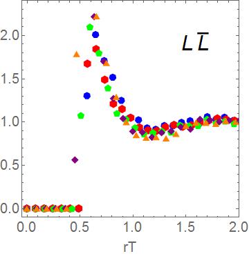
Figure 1: (Color online) The correlation of $L\bar{L}$ pair versus the distance $rT$. Here, and in all other plots, the points correspond to the following temperatures $T/T_{c}(color,polygon)=0.66(blue,7)$, $0.78(red,6)$, $0.92(green,5)$ , $1.09(purple,4)$, $1.28(orange,3)$, in units of $T_{c}$. Triangle is the highest temperature.

The correlation function for the $M\bar{M}$ dyon channel is shown in Fig. 2. Note that this channel has periodic rather than antiperiodic quark zero modes. This means that, unlike the previous case, the $M$-type dyons do not become ’t Hooft effective vertices, and their correlator does not include any quark exchanges. It indeed displays a similar core, but much smaller correlations. Those are induced by the classical (leading order) gluonic attraction studied in Larsen:2014yya . Their large-distance asymptotics should thus provide a combination of electric and magnetic screening masses, which are $m/T_{c}\sim 2$.

Note that unlike the $L\bar{L}$ correlator, the $M\bar{M}$ one shows a systematic temperature dependence. The highest $T$, shown by triangles, show the strongest correlations. This happens because the classical (leading order) interaction is $\sim 1/g^{2}(T)\sim log(T)$ gets stronger at high $T$. Indeed, the object discussed are “magnetic”, thus this unusual direction of running of their effective correlations.

The last dyon channel we study is the $ML$ one, corresponding to the instanton-forming pair. It is the so called Bogomolny-Prasad-Sommerfeld (BPS) protected channel, in which the classical (leading order) interaction between the dyons vanishes. The correlation function shown in Fig. 3 does not have the classical core, and is concentrated at significantly smaller distances than other two: perhaps indicating the instanton formation. The observed effect is due to the one-loop interaction studied by Diakonov et al Diakonov:2004jn and implemented in our partition function.

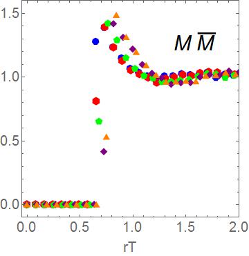
Figure 2: (Color online) The correlation of $M\bar{M}$ pair versus the distance $rT$. The different points corresponds to different temperatures as explained in Fig. 1.

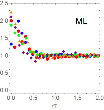
Figure 3: (Color online) The correlation of $ML$ pair versus the distance $rT$. The different points corresponds to different temperatures as explained in Fig. 1.

III The fluctuations

III.1 The setting

Lattice gauge theories are traditionally defined on a 4-dimensional torus, by imposing periodic boundary conditions for all 4 coordinates. The same geometry has been used for the instanton liquid simulations. Recent studies of the instanton-dyon ensemble have been done using the $S^{3}$ sphere. The global charges – e.g. magnetic $M$ and electric $E$ – are fixed by the amount of dyons, and thus cannot fluctuate.

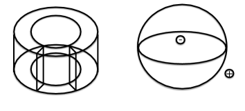
Figure 4: (left) A sketch of the torus with the subvolumes cut out; (right) The subvolumes of the $S^{3}$ sphere are, after a stereographic projection, the interior and exterior of the $S^{2}$ sphere as shown. The indicated $\pm$ charges can now be separated as shown.

Cutting the torus by two planes, as shown in Fig. 4(left), one can obtain variable $subvolumes$ $V_{4}$. Note that those have $constant$ area $A_{3}$. Therefore, the result of studies of the fluctuation of $Q$ in the instanton ensemble with light fermions, reproduced in Fig. 5, at large volume becomes horizontal (volume-independent). If the volume in question, e.g. the 4-d torus used in lattice or the $S^{3}$ used in the instanton-dyon simulations, has a boundary, like in sub-volumes to be discussed, the fluctuations occur near it, basically in the volume

$$V_{fluct}\sim A_{boundary}R_{screening}$$ (1)

Figure 5: An example of the susceptibility in sub-box $\chi_{sublat}$ as a function of the fraction of the total box, $x/L$, from Shuryak:1994rr . The thin parabolic line corresponds to randomly placed instantons and antiinstantons, the dots are for the interacting instanton liquid. Strong screening of the topological charge in this model is evident. Thin lines show different fits, from which the value of $m_{\eta^{\prime}}$ was extracted.

The setting of the instanton-dyon simulations we will study is different. The $S^{3}$ sphere, imbedded into 4-d space, can be cut into two parts by a $single$ plane. It is convenient to think about the stereographic projection of this sphere back to the 3-d space. The resulting boundary is the $S^{2}$ sphere, with the 3-d subvolumes being its interior and exterior space, as shown in Fig. 4(right). We remind that the volumes of both subvolumes are finite, see details in the appendix. When the radius of the boundary grows, its area reaches a maximum, at the angle $\psi=\pi/2$, and then decreases, due to the $r$-dependent factor induced by the stereographic projection.

III.2 The fluctuating charges

One can either study fluctuations of each dyon type, or of their particular combinations. We propose instead to focus on the fluctuations of the following global quantum numbers, the topological charge $Q$, the magnetic and electric charges $M$ and $E$, and the action $S$

$$\chi_{Q}=<Q^{2}>$$

$$\chi_{M}=<M^{2}>$$

$$\chi_{E}=<E^{2}>-<E>^{2}$$ (2)

$$\chi_{S}=<S^{2}>-<S>^{2}$$

Note that the last two have a non-zero VEV, which needs to be subtracted. The average magnetic charge $<M>=0$ because dyon ensembles have equal number of dyons and anti-dyons. The electric charge is different, because in general $n_{M}\neq n_{L}$.

The former one is the well known topological susceptibility, long studied on the lattice. Its usual definition includes division by the 4-volume $V_{4}$ and the limit $V_{4}\rightarrow\infty$, which eliminates the dependence on the volume shape. As it was already emphasized in Shuryak:1994rr , not only is this limit unnecessary, the study of the fluctuations dependence on the volume shape and size reveals such valuable information as the screening lengths for the corresponding charges. For $Q$ it is known as the $\eta^{\prime}$ mass, and for $M,E$ as the magnetic and electric screening masses $m_{M},m_{E}$ – all three subject for separate lattice measurements.

Let us further remind that in QCD-like theories with light quarks the topological susceptibility vanishes in the chiral limit $m\rightarrow 0$ and is suppressed by the powers of the nonzero quark masses, $O(m)$ at $T<T_{c}$ and $O(m^{N_{f}})$ at $T>T_{c}$. The latter is just the suppression due to ’t Hooft zero modes.

At high $T>2T_{c}$ the VEV of the Polyakov line $<P>\approx 1$ and the nontrivial holonomy fields are practically absent. That means the topological objects are the $instantons$ (or, more precisely, their finite-$T$ version known as calorons). Since at such $T$ the instanton actions are large and density exponentially small, one expects, and indeed observes on the lattice, that the topological ensemble is represented by the Dilute Instanton Ensemble (DIE). Diluteness leads to the Poisson statistics of fluctuations, and thus $\chi_{Q}$ basically gives us the instanton density.

At lower $T<300-400\,MeV$, the VEV of the Polyakov line takes some values between 1 and 0, and the appropriate ensemble should be described in terms of the instanton-dyons. While all of them have the topological charge $Q$, only “twisted” $L$-kind have fermionic zero modes. Therefore, fluctuations of $Q$ and fermion mass suppression should in principle become decoupled. In particularly, in the chiral limit there should be a non-zero $\chi_{Q}$ due to $M$-type dyons.

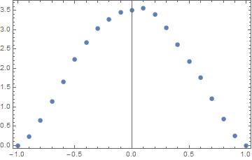
Figure 6: The mean topological charge squared $<Q^{2}>$ in a subvolume, versus the cut parameter $cos(\psi_{cut})$.

III.3 Fluctuations in the instanton-dyon ensemble

In Fig. 6 we show a typical histogram, displaying fluctuation of the topological charge $<Q^{2}>$ as a function of the size of the subvolume. It has a characteristic symmetric shape, because fluctuations in a small volume and in a complementary volume which includes the whole sphere without a small part, are identical.

In order to understand them better, one needs to normalize such histograms to a distribution calculated for uncorrelated dyons. The uncorrelated case is only volume dependent and one can therefore write the probability for finding $n$ out of $N$ charges in a sub-volume $V$ of the total volume $V_{0}$, as

$$P(V,n) = \frac{N!}{n!(N-n)!}\left(\frac{V}{V_{0}}\right)^{n}\left(1-\frac{V}{V_{0}}\right)^{N-n}$$ (3)

Which gives the fluctuation when summed over the charge squared for all $n$.

The resulting plots are shown in Fig. 7. Note, that if the ensemble be an ideal gas, by definition all plots should show values equal to one.

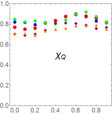
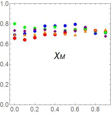
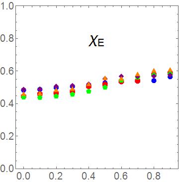
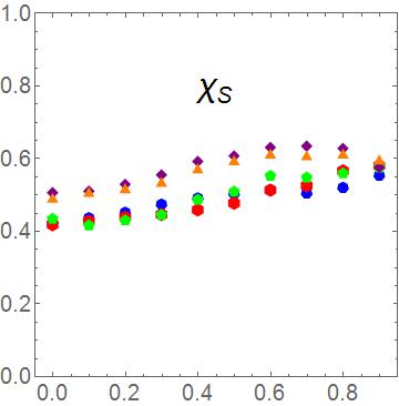
Figure 7: (Color online) The normalized fluctuations of the topological charge $Q$, the magnetic charge $M$, the electric charge $E$ and the action $S$, as a function of subvolume cut $cos(\psi_{cut})$. Because of symmetry of the distributions, only one half of it is shown. The l.h.s., $cos(\psi_{cut})=0$ corresponds to cutting the sphere into two equal halfs, the r.h.s. at $cos(\psi_{cut})\rightarrow 1$ corresponds to cutting off a very small part. The different points corresponds to different temperatures as explained in Fig. 1.

Few comments on those are in order:
(i) The fluctuations of all charges are very similar. They all seem to be of the “volume” kind, since the plots normalized to random ensemble all look rather flat.
(ii) The absolute value of the fluctuations is however not one, but smaller. This reflects presence of an attraction between opposite charges, resulting in formation of “neutral clusters”, pairs etc.
(iii) Like for the correlations discussed above, we observe only very small temperature dependence of the fluctuations.
(iv) There are visible deviations from constant value of the normalized fluctuations at the “wings” of the distributions. Those appear when the sub-volume dimension becomes comparable to the micro correlation lengths of the objects themselves.
(v) Some combinations of dyon interactions have a hard core in the ensemble. This cuts out possible small fluctuations, and is at least partially responsible for the values far off one at small volumes, ie. x-axis close to 1.

We do not try fitting those deviations for the values of the screening masses, as those were much better displayed by the correlation measurements reported above.

IV Summary and discussion

Short-range correlations between $L\bar{L}$ dyons is the channel corresponding to the $<QQ>$ correlator in the QCD vacuum, in the sense that both are related to quark-induced forces and large $\eta^{\prime}$ mass. The main conclusions one can get from our discussion of this correlation function in section II.2 are: (i) like in vacuum, this channel shows the largest screening mass; (ii) the screening effect in studied $T$ range is basically $T$-independent.

This is to be compared to the long-distance correlations associated with chiral symmetry breaking. For $T<T_{c}$ we know that there appear very long “topological clusters”, leading to very small Dirac eigenvalues, which are absent at $T>T_{c}$. So, two different approaches to the topology correlations are clearly complementary.

The $M\bar{M}$ dyon channel does not have quark exchanges. It display smaller correlations induced by classical (leading order) attraction studied in Larsen:2014yya . The $ML$ dyon channel corresponds to the instanton-forming pair. It is the so called Bogomolny-Prasad-Sommerfeld (BPS) protected channel, in which the classical (leading order) interaction between the dyons vanishes.

The second part of the paper is devoted to $fluctuations$ of certain charges in subvolumes. In principle, those should be sensitive to corresponding screening lengths, provided those are comparable with the actual dimensions of these subvolumes. However the data presented in section III do $not$ show any clear shape difference between the interacting ensemble of dyons and the random one: perhaps all of them only depend on the size of the subvolume.

These results are by no means trivial, they can and should be used in order to determine on the lattice where the transition from the instanton gas to the instanton-dyon plasma takes place. Recall that the instanton ensemble has no fluctuations of the magnetic charge at all, while the instanton-dyon plasma predicts certain relations between topological and magnetic charges, as shown above. The instanton ensemble in the chiral limit $m_{q}\rightarrow 0$ has no $\chi$ proportional to the volume, since single instantons in this limit disappear. The instanton-dyon ensemble, on the other hand, even in the chiral limit, has non-zero $\chi$ fluctuations due to $M$-dyons.

Appendix A The instanton-dyon ensemble

This section contain brief reminder of the model used. The so called instanton-dyons are instanton constituents. Their sizes and actions depend on one crucial parameter, the so called holonomy value $\nu(T)$, related to the mean value of the Polyakov line. At high $T>2T_{c}$ the VEV of the Polyakov line $<P>\approx 1$ and the holonomy disappears, $\nu\approx 0$. At $T<T_{c}$ $<P>\approx 0$ and the holonomy takes the so called “confining value”. In the considered case of the $SU(2)$ color $\nu\approx 1/2$.

The two-color theory has 4 instanton-dyon types, $M,L,\bar{M},\bar{L}$. $M$ and $L$ are selfdual, the other anti-selfdual. The actions of those, and their interactions, have been defined semiclassically. Certain number of the dyons – in the ensemble used 64 of them – are put on the 3-dimensional sphere $S^{3}$. Standard Metropolis algorithm and “integration back” method are used to calculate the free energy. The value of the parameters – such as holonomy value $\nu$ and the densities of different types, $n_{M}\neq n_{L}$ – are defined from the minimum of the free energy, and thus are temperature dependent.

Briefly, about geometry of the $S^{3}$ sphere. Its volume is $V_{3}=2\pi^{2}R^{3}$, where $R$ is the radius. Since the dyon density decreases with temperature, and we keep their number fixed, this radius is also increasing with $T$.

We work with locations on the $S^{3}$ sphere using 4-dimensional unit vectors. Standard three standard polar angles $\psi,\theta,\phi$ can be used to define coordinates

$$\vec{n}=[\sin(\psi]\sin(\theta)\sin(\phi),\sin(\psi)\sin(\theta)\cos(\phi),$$

$$\sin(\psi)\cos(\theta),\cos(\psi)]$$ (4)

The corresponding metrics is

$$dl^{2}/R^{2}=d\psi^{2}+sin^{2}\psi d\theta^{2}+sin^{2}\psi sin^{2}\theta d\phi^{2},$$ (5)

and the volume element reads

$$dV=\sin^{2}(\psi)\sin(\theta)d\psi d\theta d\phi$$ (6)

Subvolumes, used in the fluctuation section, are defined via the boundary plane $\psi=\psi_{cut}$.

The points on the sphere can be mapped onto points on its equatorial plane $X^{i},i=1,2,3$ via standard stereographic projection. The subvolumes correspond to the interior and exterior of a $S^{2}$ sphere, with the radius defined by $\psi_{cut}$. The projected volume element on the plane $X^{i},i=1,2,3$ is given by a version of Riemann formula

$$dV=({2\over 1+r^{2}/R^{2}})^{3}4\pi r^{2}dr$$ (7)

The first factor makes the integral to $r=\infty$ convergent, and equal to that of the original sphere.

Appendix B Screening in the infinite volume and on the $S^{3}$ sphere

General expressions for the point-to-point 3d correlator of charges, e.g. the topological charge $Q$, takes the standard Yukawa form with a screening mass (inverse radius) $m$

$$K(|x-y|)=<Q(x)Q(y)>=$$ (8)

$$\delta(x-y)-{1\over 4\pi|x-y|}exp(-{|x-y|m})$$

in which the first term is say a positive charge and the second is its “compensated” negative charge. The normalization corresponds to the integral over either $x$ or $y$ to vanish, $<Q>=0$. This feature is also well known in the $q\rightarrow 0$ limit of its Fourier transform

$$\tilde{K}(q)=1-{1\over q^{2}R^{2}+1}={q^{2}R^{2}\over q^{2}R^{2}+1}$$ (9)

In flat space fluctuations in a subvolume $V$ can be described by the double integral

$$I_{V}=\int_{x,y\in V}d^{3}xd^{3}yK(|x-y|)$$ (10)

On the 3-dimensional sphere $S^{3}$ one needs to find the analog to the Yukawa potential. The screened Coulomb potential of a charge, placed on the north pole of the $S^{3}$ sphere $\psi=0$, can be found from the $\psi$-part of the Laplacian, which reads

$${1\over\sqrt{g}}\partial_{\mu}(\sqrt{g}g^{\mu\nu}\partial_{\nu}f)=f^{\prime\prime}(\psi)+{2\over tan(\psi)}f^{\prime}(\psi)$$ (11)

Adding the mass term, one finds the needed analogue of the Yukawa potential to be

$$f(\psi)={exp[-\sqrt{-1+m^{2}R^{2}}\psi]\over 4\pi sin(\psi)}$$ (12)

Note the presence of the second singularity at the south pole $\psi=\pi$, which is however exponentially suppressed by $exp(-mR\pi)$ and disappear for large macroscopic spheres $mR\gg 1$.

References

- (1) A. A. Belavin, A. M. Polyakov, A. S. Schwartz and Y. S. Tyupkin, Phys. Lett. 59B, 85 (1975). doi:10.1016/0370-2693(75)90163-X
- (2) T. Schafer and E. V. Shuryak, Rev. Mod. Phys. 70, 323 (1998) doi:10.1103/RevModPhys.70.323 [hep-ph/9610451].
- (3) T. C. Kraan and P. van Baal, Phys. Lett. B 435, 389 (1998) doi:10.1016/S0370-2693(98)00799-0 [hep-th/9806034].
- (4) K. M. Lee and C. h. Lu, Phys. Rev. D 58, 025011 (1998) doi:10.1103/PhysRevD.58.025011 [hep-th/9802108].
- (5) N. M. Davies, T. J. Hollowood, V. V. Khoze and M. P. Mattis, Nucl. Phys. B 559, 123 (1999) doi:10.1016/S0550-3213(99)00434-4 [hep-th/9905015].
- (6) E. Poppitz and M. Unsal, JHEP 1107, 082 (2011) doi:10.1007/JHEP07(2011)082 [arXiv:1105.3969 [hep-th]].
- (7) E. Poppitz, T. Schafer and M. Unsal, JHEP 1210, 115 (2012) doi:10.1007/JHEP10(2012)115 [arXiv:1205.0290 [hep-th]].
- (8) Y. Liu, E. Shuryak and I. Zahed, Phys. Rev. D 92, no. 8, 085006 (2015) doi:10.1103/PhysRevD.92.085006 [arXiv:1503.03058 [hep-ph]].
- (9) Y. Liu, E. Shuryak and I. Zahed, Phys. Rev. D 92, no. 8, 085007 (2015) doi:10.1103/PhysRevD.92.085007 [arXiv:1503.09148 [hep-ph]].
- (10) Y. Liu, E. Shuryak and I. Zahed, Phys. Rev. D 94, no. 10, 105011 (2016) doi:10.1103/PhysRevD.94.105011 [arXiv:1606.07009 [hep-ph]].
- (11) Y. Liu, E. Shuryak and I. Zahed, Phys. Rev. D 94, no. 10, 105012 (2016) doi:10.1103/PhysRevD.94.105012 [arXiv:1605.07584 [hep-ph]].
- (12) Y. Liu, E. Shuryak and I. Zahed, Phys. Rev. D 94, no. 10, 105013 (2016) doi:10.1103/PhysRevD.94.105013 [arXiv:1606.02996 [hep-ph]].
- (13) P. Faccioli and E. Shuryak, Phys. Rev. D 87, no. 7, 074009 (2013) doi:10.1103/PhysRevD.87.074009 [arXiv:1301.2523 [hep-ph]].
- (14) R. Larsen and E. Shuryak, Nucl. Phys. A 950, 110 (2016) doi:10.1016/j.nuclphysa.2016.03.013 [arXiv:1408.6563 [hep-ph]].
- (15) R. Larsen and E. Shuryak, Phys. Rev. D 92, no. 9, 094022 (2015) doi:10.1103/PhysRevD.92.094022 [arXiv:1504.03341 [hep-ph]].
- (16) R. Larsen and E. Shuryak, Phys. Rev. D 93, no. 5, 054029 (2016) doi:10.1103/PhysRevD.93.054029 [arXiv:1511.02237 [hep-ph]].
- (17) R. Larsen and E. Shuryak, Phys. Rev. D 94, no. 9, 094009 (2016) doi:10.1103/PhysRevD.94.094009 [arXiv:1605.07474 [hep-ph]].
- (18) E. Shuryak, arXiv:1610.08789 [nucl-th].
- (19) C. Bonati, et al., JHEP 03 (2016) 155. arxiv 1612.06269
- (20) S. Borsanyi, et al., Phys. Lett. B752 (2016) 175 181. Nature 539, no. 7627, 69 (2016) doi:10.1038/nature20115 [arXiv:1606.07494 [hep-lat]].
- (21) P. Petreczky, H. P. Schadler and S. Sharma, Phys. Lett. B 762, 498 (2016) doi:10.1016/j.physletb.2016.09.063 [arXiv:1606.03145 [hep-lat]].
- (22) V. G. Bornyakov, E.-M. Ilgenfritz, B. V. Martemyanov and M. M ller-Preussker, Phys. Rev. D 93, no. 7, 074508 (2016) doi:10.1103/PhysRevD.93.074508 [arXiv:1512.03217 [hep-lat]].
- (23) E. Shuryak, arXiv:1701.08089 [hep-lat].
- (24) E. V. Shuryak and J. J. M. Verbaarschot, Phys. Rev. D 52, 295 (1995) doi:10.1103/PhysRevD.52.295 [hep-lat/9409020].
- (25) D. Diakonov, N. Gromov, V. Petrov and S. Slizovskiy, Phys. Rev. D 70, 036003 (2004) doi:10.1103/PhysRevD.70.036003 [hep-th/0404042].